Deformed Explicitly Correlated Gaussians

Abstract

Deformed correlated Gaussian basis functions are introduced and their matrix elements are calculated. These basis functions can be used to solve problems with nonspherical potentials. One example of such potential is the dipole self-interaction term in the Pauli-Fierz Hamiltonian. Examples are presented showing the accuracy and necessity of deformed Gaussian basis functions to accurately solve light-matter coupled systems in cavity QED.

I Introduction

Few-body approaches have reached very high accuracy in atomic and molecular systems Boys (1960); Singer (1960); Kołos and Wolniewicz (1963); Drake (1970); Drake and Swainson (1991); Yan and Drake (1997); Korobov (2000); Nakatsuji et al. (2007); Ryzhikh and Mitroy (1997); Bubin and Varga (2011); Bubin and Adamowicz (2004); Stanke et al. (2006); Cencek et al. (1995); Sharkey et al. (2013a, b); Kirnosov et al. (2013); Bubin et al. (2013a); Formanek et al. (2014); Sharkey and Adamowicz (2014) and these calculations proved to be indispensible explaining properties such as the electron correlationsLin (1983), relativistic effectsBubin and Varga (2011); Cencek and Kutzelnigg (1996), molecular bondsRichard (1994); Strasburger (1999); Cencek (2000), and quantum dynamics of nucleiStanke et al. (2007); Bubin et al. (2007); Pachucki and Komasa (2009); Holka et al. (2011). As an example, the accuracy of theoretical prediction Puchalski et al. (2019) and experimental measurement Hölsch et al. (2019) has reached the level of 1 MHz for the dissociation energy of the H₂ molecule. The accuracy allows benchmarking the theory against measurement to answer fundamental questions (e.g. about the nature of the physical constants) and the development of accurate approximations for efficient computational approaches.

Not all few-body approaches are created equal. There are approaches with distinct advantages for certain systems and well-known limitations for others. Hylleraas-type wave functions work extremely well in two- and three-electron atomic systems,Hylleraas (1928, 1929); Tang et al. (2013); Bhatia et al. (1967); Yan and Drake (1997); Ho and Yan (1999); Korobov (1996, 2000, 2002); Korobov et al. (2006); Yan et al. (2008); Wang et al. (2011) but the extension of the Hylleraas basis approach beyond three electrons is very tedious because the analytical calculation of the matrix elements King et al. (2011) is difficult. Hyperspherical approaches Rakshit and Blume (2012); Lin (1974); Rittenhouse et al. (2010); Nielsen et al. (2001); Rittenhouse et al. (2010); Lin (1995); Masili et al. (1995); Tolstikhin and Matsuzawa (2001) have also been succesfully used but have similar limitations although there are new approaches to circumvent the size restrictions von Stecher and Greene (2009); Suzuki (2015); Suzuki and Varga (2018); Daily and Greene (2014); Higgins et al. (2021); Suzuki (2020).

The matrix elements of Explicitly Correlated Gaussian (ECG) can be calculated for any number of particles. Because of this, ECGs became very popular tools in high accuracy calculations Hornyák et al. (2020); Bubin and Adamowicz (2017); Hornyák et al. (2019); Sharkey et al. (2013b); Cafiero et al. (2003); Strasburger (2014); Varga et al. (1988); Tung et al. (2010); Kirnosov et al. (2013); Bubin et al. (2013a); Blume and Yan (2014); Formanek et al. (2014); Mitroy et al. (2013); Yin and Blume (2015); Salas and Varga (2014); Bubin and Varga (2011); Puchalski and Pachucki (2014a, b); Puchalski and Pachucki (2015); Sharkey and Adamowicz (2014); Mátyus and Reiher (2012); Sharkey et al. (2009a); Zaklama et al. (2020); Muolo et al. (2019-10-21); Kedziorski et al. (2020); Bubin and Adamowicz (2020-05-29); MATYUS (2013); Jeszenszki et al. (2021); Strasburger (2020); Bubin et al. (2013a); Muolo and Reiher (2020); Rowan et al. (2020); Nasiri et al. (2020); Stanke and Adamowicz (2019); Stanke et al. (2019); Møller et al. (2019); Varga (2019); Muolo et al. (2018a, b); Adamowicz et al. (2017); Bubin et al. (2017); Fedorov (2016); Joyce and Varga (2016); Bubin et al. (2016); Puchalski et al. (2015, 2014); Bubin and Prezhdo (2013); Bubin et al. (2013b); Detmold and Shanahan (2021). The practice of using ECGs as basis functions has been around since 1960 Boys (1960); Singer (1960). The quadratic form involving inter-particle distances in ECGs permits the reduction of the Hamiltonian matrix elements to very simple analytic expressions and the algebraic complexity of the matrix elements does not change with the number of particles. Further, the matrix elements can be generalized for an arbitrary angular momentum Joyce and Varga (2016); Stanke et al. (2019); Mátyus and Reiher (2012); Joyce and Varga (2016); Sharkey et al. (2009b); Varga et al. (1998); Strasburger (2014). These matrix elements depend on the Gaussian parameters of the ECGs which should be carefully optimizedKozlowski and Adamowicz (1992a); Suzuki and Varga (1998); Komasa et al. (1995); Varga (2019); Bubin et al. (2010); Tung et al. (2011); Sharkey et al. (2011a); Bubin and Adamowicz (2008) to get highly accurate variational upper bounds. The Gaussian parameters are most often chosen to be real, but the extension to complex parameters has also been tested Bubin and Adamowicz (2006); Bubin et al. (2017, 2016). Systems with periodic boundary conditions have also been investigated Yin and Blume (2013).

The wide range of applications of ECGs has been demonstrated in several recent reviewsBubin et al. (2013a); Cafiero et al. (2003); Mitroy et al. (2013). Currently, high accuracy ECG calculations are actively pursued for relatively large systems, e.g. five-body calculations of the energy of the H${}_{3}^{+}$ Muolo et al. (2019-10-21), or the Beryllium atom with finite nuclei mass Hornyák et al. (2019), or a six-particle calculation of the Boron atom Bubin and Adamowicz (2017) and the singly charged Carbon ion Hornyák et al. (2020). These calculations reached high accuracy, and using relativistic corrections are comparable to the experimental data. To reach this accuracy for large systems one needs a large basis dimension. For example, in Ref. Hornyák et al. (2019), 16000 basis functions were used. Additionally, ECGs have been applied to the nuclei in multi-cluster approximations Suzuki et al. (2008); Mikami et al. (2014); Satsuka and Horiuchi (2019); Suzuki (2021); Hiyama (2012); Aoyama et al. (2012); Suzuki et al. (2008). While these cases do not reach the same level of accuracy as the atomic and molecular cases, ECGs offer the unique advantage of treating the nuclear dynamics in an efficient way.

The ECGs are not restricted to bound state problems. More recently scattering of composite particles have also been studied using ECG’s combined with the confined variational method Zhang et al. (2021); Mitroy et al. (2008); Wu et al. (2021); Wan et al. (2021); Wu et al. (2020); Zhang et al. (2019, 2009, 2008).

There are many works that have evaluated the matrix elements of ECG’s for spherical (L = 0) cases Suzuki and Varga (1998); Kozlowski and Adamowicz (1991); Kozlowski and Adamowicz (1992b); Cencek and Rychlewski (1993, 1995); Varga and Suzuki (1995); Bubin and Adamowicz (2008); Detmold and Shanahan (2021); Yin and Blume (2013). Spherical ECGs have been used in a variety of applications, such as the study of Efimov physicsBlume and Yan (2014), hyperfine splitting Puchalski and Pachucki (2013); Puchalski and Pachucki (2014b), quantum electrodynamic correctionsPuchalski and Pachucki (2015), Fermi gases of cold atomsYin and Blume (2015), and potential energy curves Tung et al. (2010).

There are many systems where nonspherical (L $>$ 0) ECGs are necessary (e.g. polyatomic molecules or excited states of atoms), but the calculation of the matrix elements of these functions is more complicated. There are two different ways that have been proposed. In the first one the Gaussian centers are shifted, which introduces nonspherical components into the basis functions Muolo and Reiher (2020); Muolo et al. (2018a); Suzuki and Varga (1998); Strasburger (2014); Muolo et al. (2018b); Simmen et al. (2013). The advantage of this approach is that the calculation of the matrix elements remain simple, and the disadvantage is that the desired angular momentum has to be built-in Strasburger (2014, 2019, 2020) or has to be projected out Muolo and Reiher (2020); Muolo et al. (2018a).

The second possibility is to multiply the ECGs with polynomials of the interparticle coordinates. Different approaches have been developed to calculate the matrix elements in this case. For example, one can restrict the calculation for a special $L$ value, and explicitly work out the formalism for that case. For example, Refs. Sharkey et al. (2009a, 2011b, 2011a, 2011c); Sharkey et al. (2010) calculated the energy and energy gradient matrix elements for $L=1$, while Ref. Sharkey et al. (2011b) tackled D states. Alternatively, representations using “global vectors” have been put forwardSuzuki and Varga (1998); Varga and Suzuki (1995); Varga et al. (1988); Suzuki et al. (1998) and this approach has been developed further Suzuki et al. (2008); Mátyus and Reiher (2012); MATYUS (2013). In the global vector representation, a vector $\mathbf{v}$, formed as a linear combination of all particle coordinates, is used as an argument of spherical harmonics to define the orbital momentum. The coefficients in the linear combination are treated as real-valued variational parameters. The advantage of this approach is that the calculation of the matrix elements remains relatively simple. The disadvantage is that the optimization of the variational parameters is difficult, and not all possible partial wave expansion components can be readily represented.

Another approach to calculating matrix elements of non-spherical ECGs is to calculate the matrix elements of the 1D case analyticallyZaklama et al. (2020), and then generalize to 2D or 3D using tensor products if needed. The advantage of this approach is that the ECGs parameters can be different in different directions and problems with nonspherical potentials can be solved.

Finally, direct calculation of nonspherical ECG matrix elements for a general case has also been worked out Joyce and Varga (2016). In this case, the matrix elements are calculated for any desired product of single-particle coordinates.

The goal of this paper is to introduce Deformed Explicitly Correlated Gaussians (DECGs). In the DECGs, the Gaussian parameters are different in the $x,y$, and $z$ directions. In addition, we will also allow the Gaussian centers to be placed in an arbitrary position and use the position as a variational parameter. The DECGs can be used to solve problems where the potential is non-spherically symmetric.

The introcution of DECGs is motivated by the recent interest in light-matter coupled systems, particularly atoms and molecules in cavity QED Frisk Kockum et al. (2019); Flick et al. (2018); Schafer et al. (2018); Jestädt et al. (2019); Rokaj et al. (2021); Sidler et al. (2020); Schuler et al. (2020); Flick and Narang (2018); Rivera et al. (2019); Szidarovszky et al. (2018); Ashida et al. (2021); Schäfer et al. (2019); Ruggenthaler et al. (2018); Flick et al. (2015, 2017); Le Boité (2020); Hoffmann et al. (2020); Tokatly (2018). The light-matter coupled systems are usually described on the level of the Pauli-Fierz (PF) nonrelativistic QED Hamiltonian Jestädt et al. (2019); Ruggenthaler et al. (2018); Mandal et al. (2020a). In this Hamiltonian, there is a dipole self-interaction term, $(\vec{\lambda}\cdot\vec{D})^{2}$, where $\vec{\lambda}$ is the coupling vector of the photons and $\vec{D}$ is the dipole moment of the system. This term introduces a nonspherical potential into the Hamiltonian which makes the calculation difficult. The situation is somewhat reminiscent of the magnetic Hamiltonian where the potential is cylindrically symmetric and Gaussians have to be tailored to this symmetry Salas and Varga (2014); Salas et al. (2015).

The outline of this paper is as follows. Succeeding the introduction we will introduce our notation and formalism, while Secs. II.1-II.5 will provide the calculations for the overlap matrix, dipole self-interaction removal, electron-photon coupling in addition to the kinetic and potential energy operators. Numerical examples are given in Sect. III. To make the paper more easily readable, useful but not essential equations are collected in the Appendices. Atomic units are used in the paper.

II Formalism

We consider a system of $N$ particles with positions $\vec{r}_{1},...\vec{r}_{N}$, where $\vec{r}_{i}=(x_{i},y_{i},z_{i})$, and charges $q_{1},...,q_{N}$. We define

$${\mbox{\boldmath$x$}}=\left(\begin{array}[]{c}x_{1}\\ x_{2}\\ \vdots\\ x_{N}\end{array}\right)$$ (1)

and $y$ and $z$ similarly. We also define

$$\vec{\mbox{\boldmath$r$}}=\left(\begin{array}[]{c}{\mbox{\boldmath$x$}}\\ {\mbox{\boldmath$y$}}\\ {\mbox{\boldmath$z$}}\end{array}\right)=\left(\begin{array}[]{c}x_{1}\\ x_{2}\\ \vdots\\ x_{N}\\ y_{1}\\ \vdots\\ y_{N}\\ z_{1}\\ \vdots\\ z_{N}\end{array}\right)=\left(\begin{array}[]{c}r_{1}\\ r_{2}\\ \vdots\\ r_{N}\\ r_{N+1}\\ \vdots\\ r_{2N}\\ r_{2N+1}\\ \vdots\\ r_{3N}\end{array}\right).$$ (2)

So in the following $\vec{a}$ will be used for 3-dimensional vectors, and $a$ will be used for a set of single-particle coordinates in a given direction as defined by Eq. (1), and $\vec{\mbox{\boldmath$r$}}$ is a three dimensional vector formed by a set of single-particle coordinates.

A simple form of DECG functions are defined as

$$\exp\left\{-\frac{1}{2}\tilde{{\mbox{\boldmath$x$}}}A_{xx}^{k}{\mbox{\boldmath$x$}}-\frac{1}{2}\tilde{{\mbox{\boldmath$y$}}}A_{yy}^{k}{\mbox{\boldmath$y$}}-\frac{1}{2}\tilde{{\mbox{\boldmath$z$}}}A_{zz}^{k}{\mbox{\boldmath$z$}}\right\}$$ (3)

$$\times \exp\left\{-\tilde{{\mbox{\boldmath$x$}}}A_{xy}^{k}{\mbox{\boldmath$y$}}-\tilde{{\mbox{\boldmath$x$}}}A_{xz}^{k}{\mbox{\boldmath$z$}}-\tilde{{\mbox{\boldmath$y$}}}A_{yz}^{k}{\mbox{\boldmath$z$}}\right\},$$

where $A_{\alpha\beta}$ are $N\times N$ symmetric matrices. The scalar (inner) product $(\tilde{\mbox{\boldmath$a$}}\cdot\tilde{\mbox{\boldmath$b$}})$ for $N$-dimensional vectors $\tilde{\mbox{\boldmath$a$}}=(a_{1},a_{2},...,a_{N})$ and $\tilde{\mbox{\boldmath$b$}}=(b_{1},b_{2},...,b_{N})$ is to be understood as $(\tilde{\mbox{\boldmath$a$}}\cdot\tilde{\mbox{\boldmath$b$}})=\sum_{m=1}^{N}a_{m}b_{m}$. Assuming $A_{xx}=A_{yy}=A_{zz}=A$ and $A_{xy}=A_{xz}=A_{yz}=0$, one gets back the original definition of ECGs.

Now we can define the block matrix $A$ as

$$A=\left(\begin{array}[]{ccc}A_{xx}&A_{xy}&A_{xz}\\ A_{xy}&A_{yy}&A_{yz}\\ A_{xz}&A_{yz}&A_{zz}\end{array}\right),$$ (4)

and the DECG function can be written as

$$\exp\left\{-\frac{1}{2}\vec{{\mbox{\boldmath$r$}}}A^{k}\vec{{\mbox{\boldmath$r$}}}\right\},$$ (5)

where the tilde is dropped for simplicity. The superscript $k$ stands for the $k$-th basis function and

$$\vec{{\mbox{\boldmath$r$}}}A^{k}\vec{{\mbox{\boldmath$r$}}}=\sum_{i,j=1}^{3N}r_{i}A^{k}_{ij}r_{j}.$$ (6)

We multiply the simple DECG by

$$\exp\left\{\vec{{\mbox{\boldmath$r$}}}\vec{{\mbox{\boldmath$s$}}}\right\}=\exp\left\{\sum_{i=1}^{3N}s_{i}r_{i}\right\},$$ (7)

to form a basis that can describe nonzero angular momentum states and systems of multiple centers (molecules):

$$\Psi_{k}=\exp\left\{-\frac{1}{2}\vec{{\mbox{\boldmath$r$}}}A^{k}\vec{{\mbox{\boldmath$r$}}}+\vec{{\mbox{\boldmath$r$}}}\vec{{\mbox{\boldmath$s$}}}^{k}\right\}.$$ (8)

As an example, assume that we write the trial function in the following form

$${\rm exp}\left\{-{\frac{1}{2}}\sum_{i<j}^{N}\alpha_{ij}^{xx}(x_{i}-x_{j})^{2}-{\frac{1}{2}}\sum_{i<j}^{N}\alpha_{ij}^{yy}(y_{i}-y_{j})^{2}-{\frac{1}{2}}\sum_{i<j}^{N}\alpha_{ij}^{zz}(z_{i}-z_{j})^{2}\right\}$$ (9)

$$\times{\rm exp}\left\{-{\frac{1}{2}}\sum_{i,j=1}^{N}\alpha_{ij}^{xy}(x_{i}-y_{j})^{2}-{\frac{1}{2}}\sum_{i,j=1}^{N}\alpha_{ij}^{xz}(x_{i}-z_{j})^{2}-{\frac{1}{2}}\sum_{i,j=1}^{N}\alpha_{ij}^{yz}(y_{i}-z_{j})^{2}-{\frac{1}{2}}\sum_{i=1}^{N}\beta_{i}({\vec{r}_{i}-\vec{c}_{i}})^{2}\right\}.$$

In this case, we have a correlation between the particle coordinates and a single particle function centered at $\vec{c}_{i}$. The relation between the coefficients in Eq. (4) and Eq. (9) is shown in Appendix A.

II.1 Hamiltonian

The Hamiltonian of the system is

$$H=H_{e}+H_{ph}=H_{e}+H_{p}+H_{ep}+H_{d}.$$ (10)

$H_{e}$ is the electronic Hamiltonian, and $H_{p}$ is the photon Hamiltonian. The electron-photon coupling is denoted as $H_{ep}$, and the dipole self-interaction is $H_{d}$. In this case the electron-photon interaction is described by using the PF nonrelativistic QED Hamiltonian. The PF Hamiltonian can be derived Ruggenthaler et al. (2018); Rokaj et al. (2018); Mandal et al. (2020b, a); Tokatly (2018) by applying the Power-Zienau-Woolley gauge transformation Power et al. (1959), with a unitary phase transformation on the minimal coupling ($p\cdot A$) Hamiltonian in the Coulomb gauge,

$$H_{ph}={\frac{1}{2}}\sum_{\alpha=1}^{N_{p}}\left[p_{\alpha}^{2}+\omega_{\alpha}^{2}\left(q_{\alpha}-\frac{{\vec{\lambda}_{\alpha}}}{{\omega_{\alpha}}}\cdot\vec{D}\right)^{2}\right],$$ (11)

where $\vec{D}$ is the dipole operator. The photon fields are described by quantized oscillators. $q_{\alpha}={\frac{1}{\sqrt{2\omega_{\alpha}}}}(\hat{a}^{+}_{\alpha}+\hat{a}_{\alpha})$ is the displacement field and $p_{\alpha}$ is the conjugate momentum. This Hamiltonian describes $N_{p}$ photon modes with frequency $\omega_{\alpha}$ and coupling $\vec{\lambda}_{\alpha}$. The coupling term is usually written as Ruggenthaler et al. (2014)

$$\vec{\lambda}_{\alpha}=\sqrt{4\pi}\,S_{\alpha}(\vec{r})\vec{e}_{\alpha},$$ (12)

where $S_{\alpha}(\vec{r})$ is the mode function at position $\vec{r}$ and $\vec{e}_{\alpha}$ is the transversal polarization vector of the photon modes.

The electronic Hamiltonian is the usual Coulomb Hamiltonian and the three components of the electron-photon interaction are as follows: The photonic part is

$$H_{p}=\sum_{\alpha=1}^{N_{p}}\left(\frac{1}{2}p_{\alpha}^{2}+\frac{\omega_{\alpha}^{2}}{2}q_{\alpha}^{2}\right)=\sum_{\alpha=1}^{N_{p}}\omega_{\alpha}\left(\hat{a}_{\alpha}^{+}\hat{a}_{\alpha}+\frac{1}{2}\right),$$ (13)

and the interaction term is

$$H_{ep}=-\sum_{\alpha=1}^{N_{p}}\omega_{\alpha}q_{\alpha}\vec{\lambda}_{\alpha}\cdot\vec{D}=-\sum_{\alpha=1}^{N_{p}}\sqrt{\frac{\omega_{\alpha}}{2}}(\hat{a}_{\alpha}+\hat{a}_{\alpha}^{+})\vec{\lambda}_{\alpha}\cdot\vec{D}.$$ (14)

Only photon states $|n_{\alpha}\rangle$, $|n_{\alpha}\pm 1\rangle$ are connected by $\hat{a}_{\alpha}$ and $\hat{a}_{\alpha}^{+}$. The matrix elements of the dipole operator $\vec{D}$ are only nonzero between spatial basis functions with angular momentum $l$ and $l\pm 1$ in 3D or $m$ and $m\pm 1$ in 2D.

The dipole self-interaction is defined as

$$H_{d}={\frac{1}{2}}\sum_{\alpha=1}^{N_{p}}\left(\vec{\lambda_{\alpha}}\cdot\vec{D}\right)^{2},$$ (15)

and the importance of this term for the existence of a ground state is discussed in Ref. Rokaj et al. (2018).

In the following, we will assume that there is only one important photon mode with frequency $\omega$ and coupling $\vec{\lambda}$. Thus the suffix $\alpha$ is omitted in what follows. The formalism can be easily extended for many photon modes but here we concentrate on calculating the matrix elements and it is sufficient to use a single-mode.

For one photon mode Eqs. (13) (14) and (15) can be simplified and the Hamiltonian becomes

$$H=T+V+U+\omega\left(\hat{a}^{+}\hat{a}+{1\over 2}\right)+\omega\vec{\lambda}\cdot\vec{D}q+{\frac{1}{2}}(\vec{\lambda}\cdot\vec{D})^{2},$$ (16)

where $T$ is the kinetic operator

$$T=-\frac{1}{2}\sum_{i=1}^{N}\left(\frac{\partial^{2}}{\partial x_{i}^{2}}+\frac{\partial^{2}}{\partial y_{i}^{2}}+\frac{\partial^{2}}{\partial z_{i}^{2}}\right).$$ (17)

$V$ is the Coulomb interaction

$$V=\sum_{i<j}V_{c}(\vec{r}_{i}-\vec{r}_{j}),\ \ \ \ \ \ V_{c}(\vec{r}_{i}-\vec{r}_{j})={\frac{q_{i}q_{j}}{|\vec{r}_{i}-\vec{r}_{j}|}}.$$ (18)

$U$ is an external potential

$$U=\sum_{i=1}^{N}U(\vec{r}_{i}),$$ (19)

and the dipole moment $\vec{D}$ of the system is defined as

$$\vec{D}=\sum_{i=1}^{N}q_{i}\vec{r}_{i}.$$ (20)

The operators act in real space, except $q$ which acts on the photon space

$$q|n\rangle = \frac{1}{\sqrt{2\omega}}\left(a+a^{+}\right)|n\rangle$$

$$= \frac{1}{\sqrt{2\omega}}\left(\sqrt{n}|n-1\rangle+\sqrt{n+1}|n+1\rangle\right).$$

In the following, we calculate the matrix elements of DECGs. Most of the matrix elements calculated previously for ECGs remain the same except the one that uses the DECG block matrix.

II.2 Overlap matrix

The overlap matrix is given by

$$\langle\Psi_{i}|\Psi_{j}\rangle=\int\exp\left\{-\frac{1}{2}{\vec{\mbox{\boldmath$r$}}}A{\vec{\mbox{\boldmath$r$}}}+{\vec{\mbox{\boldmath$r$}}}{\vec{\mbox{\boldmath$s$}}}\right\}d{\vec{\mbox{\boldmath$r$}}},$$ (22)

where $A$ and $\vec{s}$ are defined as

$$A=A^{i}+A^{j}\ \ \ \ \ \vec{{\mbox{\boldmath$s$}}}=\vec{{\mbox{\boldmath$s$}}}^{\,i}+\vec{{\mbox{\boldmath$s$}}}^{\,j},$$ (23)

and can be calculated using Eq. (69) in Appendix B:

$$\langle\Psi_{i}|\Psi_{j}\rangle={\frac{(2\pi)^{3N/2}}{({\rm det}A)^{1/2}}}\exp\left\{\frac{1}{2}\vec{{\mbox{\boldmath$s$}}}A^{-1}\vec{{\mbox{\boldmath$s$}}}\right\}.$$ (24)

II.3 Kinetic energy

We will write the kinetic energy operator in the following form

$$T={\vec{\mbox{\boldmath$p$}}}\Lambda{\vec{\mbox{\boldmath$p$}}},$$ (25)

where the momentum operator is given by

$$p_{i}=-i\hbar{\frac{\partial}{\partial r_{i}}}\ \ \ \ \ (i=1,...,3N).$$ (26)

For a system of particles with masses $m_{1},...,m_{N}$, $\Lambda$ is a block diagonal matrix

$$\Lambda=\left(\begin{array}[]{ccc}\Lambda^{x}&0&0\\ 0&\Lambda^{y}&0\\ 0&0&\Lambda^{z}\end{array}\right),$$ (27)

where the matrix elements of the block diagonal matrix are given by

$$\Lambda^{\alpha}_{ij}={\frac{1}{2m_{i}}}\delta_{ij},$$ (28)

for systems where the external potential fixes the center of the system (e.g. electrons in a harmonic oscillator potential, or electrons in an atom where the mass of the nucleus is taken to be infinity). Otherwise, we have to remove the center of mass motion of the system using

$$\Lambda^{\alpha}_{ij}={\frac{1}{2m_{i}}}\delta_{ij}-{\frac{1}{2M}},$$ (29)

where $M=m_{1}+m_{2}+...m_{N}$. In principle $\Lambda^{x}$, $\Lambda^{y}$ and $\Lambda^{z}$ can be different if the masses of particles depend on the directions.

Taking the derivative on the right-hand side

$${\frac{\partial}{\partial r_{i}}}\exp\left\{-\frac{1}{2}\vec{{\mbox{\boldmath$r$}}}A^{j}\vec{{\mbox{\boldmath$r$}}}+{\vec{\mbox{\boldmath$r$}}}{\vec{\mbox{\boldmath$s$}}}\right\}=\left(-(A^{j}\vec{\mbox{\boldmath$r$}})_{i}+s_{i}\right)\exp\left\{-\frac{1}{2}\vec{{\mbox{\boldmath$r$}}}A^{j}\vec{{\mbox{\boldmath$r$}}}+{\vec{\mbox{\boldmath$r$}}}{\vec{\mbox{\boldmath$s$}}}\right\}.$$ (30)

Using analogous results on the left side, the overlap with the kinetic energy operator can be given by

$$\langle\Psi_{i}|T|\Psi_{j}\rangle = \int\left(\vec{{\mbox{\boldmath$r$}}}(A^{i}\Lambda A^{j})\vec{{\mbox{\boldmath$r$}}}+\vec{{\mbox{\boldmath$s$}}}^{\,i}\Lambda\vec{{\mbox{\boldmath$s$}}}^{\,j}-\vec{{\mbox{\boldmath$s$}}}^{\,i}\Lambda A^{j}\vec{{\mbox{\boldmath$r$}}}-A^{i}\vec{{\mbox{\boldmath$r$}}}\Lambda\vec{{\mbox{\boldmath$s$}}}^{\,j}\right)\exp\left\{-\frac{1}{2}\vec{{\mbox{\boldmath$r$}}}A\vec{{\mbox{\boldmath$r$}}}+{\vec{\mbox{\boldmath$r$}}}{\vec{\mbox{\boldmath$s$}}}\right\}d\vec{\mbox{\boldmath$r$}}$$ (31)

$$= \left({\rm Tr}(A^{i}\Lambda A^{k}A^{-1})-\vec{{\mbox{\boldmath$y$}}}\Lambda\vec{{\mbox{\boldmath$y$}}}\right)\langle\Psi_{i}|\Psi_{j}\rangle,$$

where we used Eqs. (70) and (B) and define $\vec{y}$ as

$$\vec{{\mbox{\boldmath$y$}}}=A^{j}A^{-1}{\vec{\mbox{\boldmath$s$}}}^{\,i}-A^{i}A^{-1}{\vec{\mbox{\boldmath$s$}}}^{\,j}.$$ (32)

II.4 Potential energy

Both $V_{c}$ and $U$ can be rewritten using a $\delta$ function,

$$V_{c}(\vec{r}_{i}-\vec{r}_{j})=\int\delta(\tilde{w}^{ij}\vec{\mbox{\boldmath$r$}}-{\vec{r}})V_{c}(\vec{r})d\vec{r},$$ (33)

where $\tilde{w}^{ij}\vec{\mbox{\boldmath$r$}}$ is a short-hand notation for $\sum_{k=1}^{N}w^{ij}_{k}{\vec{r}}_{k}$ and in this case $w^{ij}_{k}=\delta_{ik}-\delta_{jk}$. The corresponding formula for $U$ is

$$U(\vec{r}_{i})=\int\delta(\tilde{w}^{i}\vec{\mbox{\boldmath$r$}}-{\vec{r}})U(\vec{r})d\vec{r},$$ (34)

with $w^{i}_{k}=\delta_{ik}$. This form allows us to calculate the matrix elements for $\delta(\tilde{w}\vec{\mbox{\boldmath$r$}}-{\vec{r}})$ for a general case without using the particular form of the potential, and to calculate the matrix element of the potential by integration over ${\vec{r}}$. The $\delta$ function can be represented by (we drop the superscript $ij$ and $i$ of $w$ for simplicity)

$$\delta(\tilde{w}\vec{\mbox{\boldmath$r$}}-{\vec{r}})={\frac{1}{(2\pi)^{3}}}\int{\rm e}^{i\vec{k}(\tilde{w}\vec{\mbox{\boldmath$r$}}-{\vec{r}})}d{\vec{k}}.$$ (35)

We want to calculate the matrix elements

$$\langle\Psi_{i}|\delta(\tilde{w}\vec{\mbox{\boldmath$r$}}-{\vec{r}})|\Psi_{j}\rangle={\frac{1}{(2\pi)^{3}}}\int\int{\rm e}^{i\vec{k}(\tilde{w}\vec{\mbox{\boldmath$r$}}-{\vec{r}})}\exp\left\{-\frac{1}{2}\vec{{\mbox{\boldmath$r$}}}A\vec{{\mbox{\boldmath$r$}}}+\vec{{\mbox{\boldmath$r$}}}\vec{{\mbox{\boldmath$s$}}}\right\}d\vec{\mbox{\boldmath$r$}}d{\vec{k}}.$$ (36)

This can be done by defining $\vec{t}$ as

$$\vec{\mbox{\boldmath$t$}}=\left(\begin{array}[]{c}ik_{1}\tilde{w}\\ ik_{2}\tilde{w}\\ ik_{3}\tilde{w}\end{array}\right)+\vec{{\mbox{\boldmath$s$}}}.$$ (37)

Using Eq. (69), we can express the matrix element as

$$\langle\Psi_{i}|\delta(\tilde{w}\vec{\mbox{\boldmath$r$}}-{\vec{r}})|\Psi_{j}\rangle = {\frac{1}{(2\pi)^{3}}}\left({\frac{(2\pi)^{3N}}{{\rm det}A}}\right)^{\frac{1}{2}}\int{\rm e}^{-i\vec{k}{\vec{r}}}{\rm exp}\Big{(}{\frac{1}{2}}{{\vec{\mbox{\boldmath$t$}}}}A^{-1}\vec{\mbox{\boldmath$t$}}\Big{)}d{\vec{k}}$$ (38)

$$= {\frac{1}{(2\pi)^{3}}}\left({\frac{(2\pi)^{3N}}{{\rm det}A}}\right)^{\frac{1}{2}}\int{\rm e}^{-i\vec{k}{\vec{r}}}{\rm exp}\Big{(}-{\frac{1}{2}}{{\vec{k}}}B\vec{k}+{\frac{1}{2}}{{\vec{\mbox{\boldmath$s$}}}}A^{-1}\vec{\mbox{\boldmath$s$}}+i{{\vec{k}}}\vec{b}\Big{)}d{\vec{k}},$$

where $B$ is a $3\times 3$ matrix given by

$$B=\left(\begin{array}[]{ccc}B_{11}&B_{12}&B_{13}\\ B_{12}&B_{22}&B_{23}\\ B_{13}&B_{23}&B_{33}\end{array}\right),$$ (39)

with the matrix elements of $B$ defined as

$$B_{ij}=\sum_{k=(i-1)\cdot N+1}^{i\cdot N}\ \ \sum_{l=(j-1)\cdot N+1}^{j\cdot N}w_{k^{\prime}}A^{-1}_{kl}w_{l^{\prime}},$$ (40)

where $k^{\prime}=k-(i-1)\cdot N$ and $l^{\prime}=l-(j-1)\cdot N$. We have also defined a three dimensional vector ${\vec{b}}$:

$$b_{i}=\sum_{k=(i-1)\cdot N+1}^{i\cdot N}w_{k^{\prime}}\left(A^{-1}{\vec{\mbox{\boldmath$s$}}}\right)_{k}.$$ (41)

The last integral can again be calculated using Eq. (69) and we have

$$\langle\Psi_{i}|\delta(\tilde{w}\vec{\mbox{\boldmath$r$}}-{\vec{r}})|\Psi_{j}\rangle={\frac{1}{(2\pi)^{3/2}({\rm det}B)^{1/2}}}{\rm exp}\Big{(}-{\frac{1}{2}}(\vec{r}-{\vec{b}})B^{-1}(\vec{r}-\vec{b})\Big{)}\langle\Psi_{i}|\Psi_{j}\rangle.\ \ \ \$$ (42)

Integrating over $\vec{r}$ should give back the overlap, and using Eq. (69) one immediately gets these results. Note that Eq. (42) can also be used to calculate the single particle density. This formula is generalized for two particle density in Appendix D.

II.5 Electron-photon coupling

By introducing $\vec{q}$ as

$$\vec{\mbox{\boldmath$q$}}=\left(\begin{array}[]{c}\lambda_{1}q_{1}\\ \lambda_{1}q_{2}\\ \vdots\\ \lambda_{1}q_{N}\\ \lambda_{2}q_{1}\\ \vdots\\ \lambda_{2}q_{N}\\ \lambda_{3}q_{1}\\ \vdots\\ \lambda_{3}q_{N}\end{array}\right),$$ (43)

the relevant part of the coupling term can be written as

$$\vec{\lambda}\cdot\vec{D}={\vec{\mbox{\boldmath$q$}}}{\vec{\mbox{\boldmath$r$}}},$$ (44)

and the matrix elements of this term can be easily calculated using Eq. (70)

$$\langle\Psi_{i}|\vec{\lambda}\cdot\vec{D}|\Psi_{j}\rangle = \int\vec{\lambda}\cdot\vec{D}\exp\left\{-\frac{1}{2}\vec{{\mbox{\boldmath$r$}}}A\vec{{\mbox{\boldmath$r$}}}+{\vec{\mbox{\boldmath$r$}}}{\vec{\mbox{\boldmath$s$}}}\right\}d\vec{\mbox{\boldmath$r$}}$$ (45)

$$= \vec{{\mbox{\boldmath$q$}}}A^{-1}\vec{{\mbox{\boldmath$s$}}}\ \langle\Psi_{i}|\Psi_{j}\rangle.$$

II.6 Dipole self-interaction

The dipole self-interaction can also be readily available using Eq. (B):

$$\begin{aligned} \langle\Psi_{i}|{\frac{1}{2}}(\vec{\lambda}\cdot\vec{D})^{2}|\Psi_{j}\rangle&=\int{\frac{1}{2}}(\vec{\lambda}\cdot\vec{D})^{2}\exp\left\{-\frac{1}{2}\vec{{\mbox{\boldmath$r$}}}A\vec{{\mbox{\boldmath$r$}}}+{\vec{\mbox{\boldmath$r$}}}{\vec{\mbox{\boldmath$s$}}}\right\}d\vec{\mbox{\boldmath$r$}}\\ &={\frac{1}{2}}\left(\vec{{\mbox{\boldmath$q$}}}A^{-1}\vec{{\mbox{\boldmath$q$}}}+\left(\vec{{\mbox{\boldmath$q$}}}A^{-1}\vec{{\mbox{\boldmath$s$}}}\right)^{2}\right)\langle\Psi_{i}|\Psi_{j}\rangle.\end{aligned}$$ (46)

II.7 Eliminating the dipole self-interaction

One motivation of DECG is that the dipole self-interaction term of the Hamiltonian can be eliminated using a special choice of DECG exponentials producing a much simpler Hamiltonian.

The dipole self-interaction term is a special quadratic form and this quadratic form can be represented with DECG exponent. One can try to find a suitable $\alpha$ to eliminate the dipole self-interaction using the kinetic energy operator:

$$-\frac{1}{2}\sum_{i=1}^{3N}\left(\frac{\partial^{2}}{\partial r_{i}^{2}}\right)\exp\left(\alpha(\vec{\lambda}\cdot\vec{D})^{2}\right).$$ (47)

To solve this we need to evaluate the second derivative of the exponential with respect to $\vec{r}_{i}$. The first derivative with respect to $x_{i}$ is given by

$$\frac{\partial}{\partial x_{i}}\exp\left(\alpha(\vec{\lambda}\cdot\vec{D})^{2}\right)=2\alpha\lambda_{1}{q}_{i}(\vec{\lambda}\cdot\vec{D})\exp\left(\alpha(\vec{\lambda}\cdot\vec{D})^{2}\right),$$ (48)

and the second derivative

$$\frac{\partial^{2}}{\partial x_{i}^{2}}\exp\left(\alpha(\vec{\lambda}\cdot\vec{D})^{2}\right) = 2\alpha\lambda_{1}^{2}{q}_{i}^{2}\exp\left(\alpha(\vec{\lambda}\cdot\vec{D})^{2}\right)$$

$$+ 4\alpha^{2}\lambda_{1}^{2}{q}_{i}^{2}(\vec{\lambda}\cdot\vec{D})^{2}\exp\left(\alpha(\vec{\lambda}\cdot\vec{D})^{2}\right),$$

with similar expressions for $y_{i}$ and $z_{i}$. By choosing $\alpha$ as

$$\alpha=\frac{1}{2\sqrt{\sum_{i=1}^{N}{q}_{i}^{2}}\,\lambda},$$ (50)

where $\lambda$ is the magnitude of $\vec{\lambda}$, we can express the kinetic energy operator acting on the exponential as

$$-\frac{1}{2}\sum_{i=1}^{3N}\left(\frac{\partial^{2}}{\partial r_{i}^{2}}\right)\exp\left(\alpha(\vec{\lambda}\cdot\vec{D})^{2}\right)=-\left({\frac{1}{4\alpha}}+{\frac{1}{2}}(\vec{\lambda}\cdot\vec{D})^{2}\right)\exp\left(\alpha(\vec{\lambda}\cdot\vec{D})^{2}\right).$$ (51)

This means that by multiplying the basis with the factor

$$\exp\left(\alpha(\vec{\lambda}\cdot\vec{D})^{2}\right),$$ (52)

the dipole self-interaction can be removed and the numerical solution is much simpler. In this way, the nonspherical dipole self-interaction is eliminated. In other words, it is built in the basis functions. Note that the above exponential form can be recast into a DECG, but not into an ECG. The generalization of Eq. 51 to multiphoton mode can be found in Appendix E.

III Numerical Examples

In this section, we present a few numerical examples to show that the matrix elements evaluated in this paper can be used in practical calculations. We will not fully explore the efficiency of the DECG basis, and we restrict our approach to an $A$ matrix of the form

$$A=\left(\begin{array}[]{ccc}A_{xx}&0&0\\ 0&A_{xx}&0\\ 0&0&A_{xx}\end{array}\right),$$ (53)

and the trial function is

$$\Psi_{k}=\exp\left\{-\frac{1}{2}\vec{{\mbox{\boldmath$r$}}}(A^{k}+2\alpha(\vec{\lambda}\cdot\vec{D}))\vec{{\mbox{\boldmath$r$}}}+\vec{{\mbox{\boldmath$r$}}}\vec{{\mbox{\boldmath$s$}}}^{k}\right\},$$ (54)

where $\alpha$ is defined in Eq. (50). If $\alpha=0$ then this function is the conventional ECG basis function. Nonzero $\alpha$ leads to nonzero off diagonal block matrices and the basis becomes DECG.

In these calculations, we have used the separable approximation of $1/r$ in terms of Gaussians Beylkin and Monzón (2005)

$${\frac{1}{r}}=\sum_{k}w_{k}{\rm e}^{-p_{k}r^{2}}.$$ (55)

In this way, the integral in Eq. (42) can be analytically evaluated (a numerical approach is presented in Appendix C). 89 Gaussian functions with the coefficients $w_{k}$ and $p_{k}$ (taken from Ref. Beylkin and Monzón (2005)) can approximate $1/r$ with an error less than $10^{-8}$ in the interval $[10^{-9},1]$a.u. For larger intervals, one can easily scale to coefficients. Note that this expansion uses significantly fewer terms than a Gaussian quadrature for the same accuracy Beylkin and Monzón (2005).

As a first example, we consider a 2D system of 2 electrons in a harmonic oscillator confinement potential,

$${\frac{1}{2}}\omega_{0}^{2}\sum_{i=1}^{2}\vec{r}_{i}^{\,2},$$ (56)

interacting via a Coulomb potential. This problem is analytically solvable Huang et al. (2021) and we will compare the ECG ($\alpha=0$) and DECG solution. We take $\omega=0$ in Eq. (16), so there is no coupling to photons but the potential is nonspherical because $\lambda\neq 0$. We test two $\lambda$ values: $\lambda=1$ a.u. (the energy is $E=2.7807764$ a.u.) and $\lambda=2.5$ ($E=4.2624689$). Fig. 1 shows the convergence of energy as a function of the number of basis states. Each basis state is selected by comparing 250 random parameter sets and choosing the one that minimizes the energy. The DECG converges up to 3-4 digits on a basis of 100 states. The ECG converges much slower, and for the stronger coupling ($\lambda=2.5$) the energy is 0.9 a.u. above the exact value. A larger basis dimension and more parameter optimizations would improve the results, but this already shows the general tendency and the superiority of the DECG basis. Note, that the ECG would also converge to the exact result after more optimization and much larger basis size.

The next example is a 2D H₂ molecule with nuclei fixed at distance $r$. In this case, we assume that there is only one relevant photon mode with frequency $\omega=1.5$ a.u. There are infinitely many photons with energy $n\hbar\omega$ ($n=0,1,2,...)$, but only the lowest photon states are coupled to the electronic part. We solver Eq. (16) using the lowest $n=0,..,5$ photon spaces. The energy of a 2D H atom is $E=-2$ a.u. without coupling the photons. The energy of the atom coupled to photons with $\lambda=$1.5 a.u. increases to $E=-1.71$ a.u. The increase is largely due to the dipole self energy part in Eq. (16). The probability amplitudes of the spatial wave function in photon spaces are 0.988 ($n=0$), 0.01 ($n=1)$ and 0.001 $n=2$. These are small probabilities but there is a relatively strong coupling between the electrons and light. This is shown by the fact that the energy without coupling (solely due to the dipole self-interaction and the Coulomb) is -1.67 a.u. By increasing the coupling further the energy of the H₂ increases (e.g. for $\lambda=3$, $E$=-1.15 a.u.).

Fig. 2 shows the energy of the H₂ molecule with and without coupling to light. Without coupling to light, the 2D H₂ molecule has a lowest energy at around $r$=0.35 a.u. The the H₂ molecule to light the energy minimum slightly shifts toward shorter distances. Overall the three curves are very similar except that the dipole self-interaction term pushes them higher with increasing $\lambda$. The binding energies at the minimum energy point increase with $\lambda$: $E_{b}$=1.34 a.u. ($\lambda=0$), $E_{b}=1.47$ ($\lambda=1.5$ a.u.), and $E_{b}=1.68$ a.u. ($\lambda=3$ a.u.), where $E_{b}$ is the difference of the energy of the molecule and two times the energy of the H atom.

The final example is the H^- ion with finite ($m_{H}=1836.1515$ a.u.) and infinite nuclear mass in 3D. Fig. 3 shows the energy of the H atom and H^- ion as a function of $\lambda$. As the figure shows, the H^- dissociates for strong $\lambda$ in the finite mass case but remains stable in the infinite mass case. In the finite mass case, the dissociation happens around $\lambda=0.08$ a.u., at that point, the energy of the H plus an electron system becomes lower than that on H^- (the energy of the electron coupled to light is calculated by solving Eq. (16) for the electron). This example shows the importance of explicit treatment of the system as a three-body system because the light strongly couples to the proton as well.

IV Summary

We have introduced a new variant of ECG basis functions that are suitable for problems with nonspherical potentials. All necessary matrix elements are calculated and numerically tested. The treatment of the Coulomb interaction is more complicated than in the conventional ECG case due to the nonspherical integrals that appear in the interaction part. Two ways are proposed to solve this problem. One can either expand the Coulomb potential in Gaussians and the integration becomes analytical, or use numerical integration.

We have shown that using the DECG basis the coupled light-matter equations can be efficiently solved even when the coupling and thus the dipole self-interaction term is large. This opens up the way to calculate light-matter coupled few-body systems with high accuracy in cavity QED systems.

The approach might be useful in other problems with nonspherical potentials e.g. calculation of atoms and molecules in magnetic fields.

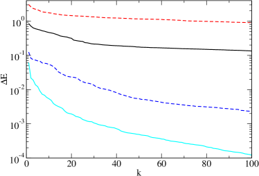
Figure 1: Energy convergence as a function of basis dimension. $\Delta E$ is the difference of the calculated energy and the exact energy. The lower two curves are DECG calculations for $\lambda=1$ a.u. (solid line), $\lambda=2.5$ a.u. (dashed line); the upper two curves are ECG calculations for $\lambda=1$ a.u. (solid line), $\lambda=2.5$ a.u. (dashed line).

Figure 2: Energy of the 2D H₂ molecule as a function of the proton-proton distance.

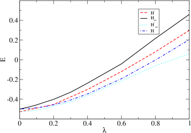
Figure 3: Energy of the 3D H^- ion as a function of $\lambda$ ($\omega=0.8$ a.u.

Appendix A Relating different forms of basis functions

In this appendix we show how Eq. (8) and Eq. (9) can be related and how the matrix elements of the trial function can be determined.

$$\begin{array}[]{l}\begin{aligned} \Psi&=\exp\left\{-\frac{1}{2}\sum_{i<j}^{N}\alpha_{ij}^{xx}\left(x_{i}-x_{j}\right)^{2}-\frac{1}{2}\sum_{i<j}^{N}\alpha_{ij}^{yy}\left(y_{i}-y_{j}\right)^{2}-\frac{1}{2}\sum_{i<j}^{N}\alpha_{ij}^{zz}\left(z_{i}-z_{j}\right)^{2}\right\}\\ &\times\exp\left\{-\frac{1}{2}\sum_{i,j=1}^{N}\alpha_{ij}^{xy}\left(x_{i}-y_{j}\right)^{2}-\frac{1}{2}\sum_{i,j=1}^{N}\alpha_{ij}^{xz}\left(x_{i}-z_{j}\right)^{2}-\frac{1}{2}\sum_{i,j=1}^{N}\alpha_{ij}^{yz}\left(y_{i}-z_{j}\right)^{2}-\frac{1}{2}\sum_{i=1}^{N}\beta_{i}\left(\vec{r}_{i}-\vec{c}_{i}\right)^{2}\right\}.\end{aligned}\end{array}$$ (57)

The diagonal blocks of the trial function evaluate to

$$\sum_{i<j}^{N}\alpha_{ij}^{xx}\left(x_{i}-x_{j}\right)^{2}={\mbox{\boldmath$x$}}M_{xx}\mbox{\boldmath$x$},$$ (58)

where $M_{xx}$ is an $N\times N$ symmetric matrix:

$$\left(M_{xx}\right)_{ii}=\sum_{\begin{subarray}{c}k=1\\ k\neq i\end{subarray}}^{N}\alpha_{ik}^{xx},\quad\left(M_{xx}\right)_{ij}=-\alpha_{ij}^{xx}\quad\text{ for }i\neq j.$$ (59)

Here, $\alpha_{ji}^{xx}$ for $j>i$ is set equal to $\alpha_{ij}^{xx}$. The off-diagonal blocks of the trial function evaluate to

$$\sum_{i,j=1}^{N}\alpha_{ij}^{xy}\left(x_{i}-y_{j}\right)^{2}={\mbox{\boldmath$x$}}G_{xx}^{xy}\mbox{\boldmath$x$}+{\mbox{\boldmath$y$}}G_{yy}^{xy}\mbox{\boldmath$y$}+{\mbox{\boldmath$x$}}G_{xy}^{xy}\mbox{\boldmath$y$}+{\mbox{\boldmath$y$}}{G_{xy}^{xy}}\mbox{\boldmath$x$},$$ (60)

where $G_{xx}^{xy}$ and $G_{yy}^{xy}$ are both diagonal,

$$\left(G_{xx}^{xy}\right)_{ii} =\sum_{j=1}^{N}\alpha_{ij}^{xy},$$ (61)

$$\left(G_{yy}^{xy}\right)_{ii} =\sum_{i=1}^{N}\alpha_{ij}^{xy},$$

while $G_{xy}^{xy}$ is defined as

$$\left(G_{xy}^{xy}\right)_{ij}=-\alpha_{ij}^{xy}(\text{ for }i,j=1,\ldots,N).\\$$ (62)

The single-particle product element of the trial function is

$$\sum_{i=1}^{N}\beta_{i}\left(\vec{r}_{i}-\vec{c}_{i}\right)^{2} =\sum_{i=1}^{N}\beta_{i}\left[\left(x_{i}^{2}+y_{i}^{2}+z_{i}^{2}\right)-2\vec{c}_{i}\cdot\vec{r}_{i}+\vec{c}_{i}\cdot\vec{c}_{i}\right]$$ (63)

$$={\mbox{\boldmath$x$}}B\mbox{\boldmath$x$}+{\mbox{\boldmath$y$}}B\mbox{\boldmath$y$}+{\mbox{\boldmath$z$}}B\mbox{\boldmath$z$}$$

$$-2\sum_{i=1}^{N}\beta_{i}\vec{c_{i}}\cdot\vec{r_{i}}+\sum_{i=1}^{N}\beta_{i}\vec{c_{i}}\cdot\vec{c_{i}},$$

where $B$ is an $N\times N$ diagonal matrix with $B_{ii}=\beta_{i}$, and

$$\sum_{i=1}^{N}\beta_{i}\vec{c_{i}}\cdot\vec{r_{i}}=\sum_{i=1}^{N}\beta_{i}\left(c_{i_{x}}x_{i}+c_{i_{y}}y_{i}+c_{i_{z}}z_{i}\right)={\vec{\mbox{\boldmath$s$}}}\cdot\vec{\mbox{\boldmath$r$}}.$$ (64)

Here, ${\vec{\mbox{\boldmath$s$}}}=\left(\beta_{1}c_{1_{x}},\beta_{2}c_{2_{x}},\ldots,\beta_{N}c_{N_{x}},\beta_{1}c_{1_{y}},\beta_{2}c_{2_{y}},\ldots,\beta_{N}c_{N_{y}},\beta_{1}c_{1_{z}},\beta_{2}c_{2_{z}},\ldots,\beta_{N}c_{N_{z}}\right).$ Combining the above results leads to

$$\Psi=\exp\left\{-\frac{1}{2}{\vec{\mbox{\boldmath$r$}}}A\vec{\mbox{\boldmath$r$}}+{\vec{\mbox{\boldmath$s$}}}\vec{\mbox{\boldmath$r$}}-\frac{1}{2}\sum_{i=1}^{N}\beta_{i}\vec{c_{i}}\cdot\vec{c_{i}}\right\},$$ (65)

with the matrix $A$ given by

$$A=\left(\begin{array}[]{ccc}M_{xx}+G_{xx}^{xy}+G_{xx}^{xz}+B&G_{xy}^{xy}&G_{xz}^{xz}\\ G_{xy}^{xy}&M_{yy}+G_{yy}^{xy}+G_{yy}^{yz}+B&G_{yz}^{yz}\\ G_{xz}^{xz}&G_{yz}^{yz}&M_{zz}+G_{zz}^{xz}+G_{zz}^{yz}+B\end{array}\right).$$ (66)

Comparing $A$ with Eq. (4), one obtains $A_{\alpha\beta}$. For example,

$$A_{xx}=M_{xx}+G_{xx}^{xy}+G_{xx}^{xz}+B,\quad A_{xy}=G_{xy}^{xy},$$ (67)

and their matrix elements are easily obtained from the above defining equations.

Appendix B Generalized Gaussian integrals

In this appendix, we list the most important formulas for Gaussian integrals. These results are valid in $n=d\times N$dimension, where $d$ is the space dimension. Define the generating function

$$g(\vec{\mbox{\boldmath$s$}};A,\vec{\mbox{\boldmath$r$}})={\rm exp}\Big{(}-{\frac{1}{2}}{{\vec{\mbox{\boldmath$r$}}}}A\vec{\mbox{\boldmath$r$}}+{\vec{\mbox{\boldmath$s$}}}\vec{\mbox{\boldmath$r$}}\Big{)}.$$ (68)

The evaluation of a Gaussian integral of this form is given by

$$\int{\rm exp}\Big{(}-{\frac{1}{2}}{{\vec{\mbox{\boldmath$r$}}}}A\vec{\mbox{\boldmath$r$}}+{{\vec{\mbox{\boldmath$s$}}}}\vec{\mbox{\boldmath$r$}}\Big{)}d\vec{\mbox{\boldmath$r$}}=\left({\frac{(2\pi)^{n}}{{\rm det}A}}\right)^{\frac{1}{2}}{\rm exp}\Big{(}{\frac{1}{2}}{{\vec{\mbox{\boldmath$s$}}}}A^{-1}\vec{\mbox{\boldmath$s$}}\Big{)},$$ (69)

Some useful formulas related to this integral are collected below. By differentiating both sides of the above equation with respect to the $i$th component of the vector $\vec{\mbox{\boldmath$s$}}$, $s_{i}$, we obtain

$$\int r_{i}\,{\rm exp}\Big{(}-{\frac{1}{2}}{{\vec{\mbox{\boldmath$r$}}}}A\vec{\mbox{\boldmath$r$}}+{{\vec{\mbox{\boldmath$s$}}}}\vec{\mbox{\boldmath$r$}}\Big{)}d\vec{\mbox{\boldmath$r$}}\quad$$ (70)

$$=\,(A^{-1}\vec{\mbox{\boldmath$s$}})_{i}\left({\frac{(2\pi)^{n}}{{\rm det}A}}\right)^{\frac{1}{2}}{\rm exp}\Big{(}{\frac{1}{2}}{{\vec{\mbox{\boldmath$s$}}}}A^{-1}\vec{\mbox{\boldmath$s$}}\Big{)}.$$

Further differentiation with respect to $\vec{\mbox{\boldmath$s$}}_{j}$ leads us to

$$\int r_{i}r_{j}{\rm exp}\Big{(}-{\frac{1}{2}}{{\vec{\mbox{\boldmath$r$}}}}A\vec{\mbox{\boldmath$r$}}+{{\vec{\mbox{\boldmath$s$}}}}\vec{\mbox{\boldmath$r$}}\Big{)}d\vec{\mbox{\boldmath$r$}}=\left({\frac{(2\pi)^{n}}{{\rm det}A}}\right)^{\frac{1}{2}}$$

$$\times {\rm exp}\Big{(}{\frac{1}{2}}{{\vec{\mbox{\boldmath$s$}}}}A^{-1}\vec{\mbox{\boldmath$s$}}\Big{)}\Big{\{}(A^{-1})_{ij}+(A^{-1}\vec{\mbox{\boldmath$s$}})_{i}(A^{-1}\vec{\mbox{\boldmath$s$}})_{j}\Big{\}}$$

Table 1: Matrix elements, ${\cal M}=\langle g(\vec{\mbox{\boldmath$s$}}^{\prime};A^{\prime},\vec{\mbox{\boldmath$r$}})|{\cal O}|g(\vec{\mbox{\boldmath$s$}};A,\vec{\mbox{\boldmath$r$}})\rangle$, of operators ${\cal O}$ between generating functions $g$ of Eq. (68). Here we take all vectors $d$-dimensional. $\tilde{w}\vec{\mbox{\boldmath$r$}}$ is a short-hand notation for $\sum_{i=1}^{3N}w_{i}\vec{r}_{i}$. $B=A+A^{\prime}$, $\vec{\mbox{\boldmath$v$}}=\vec{\mbox{\boldmath$s$}}+\vec{\mbox{\boldmath$s$}}{\,{}^{\prime}}$. $\vec{\mbox{\boldmath$y$}}=A^{\prime}B^{-1}\vec{\mbox{\boldmath$s$}}-AB^{-1}\vec{\mbox{\boldmath$s$}}{\,{}^{\prime}}$ where the elements of $w_{i}$ from $1$ to $N$ are repeated for $N+1$ to $2N$ and $2N+1$ to $3N$. $P$ is a permutation operator and the matrix $T_{P}$ is defined by $P\vec{\mbox{\boldmath$r$}}=T_{P}\vec{\mbox{\boldmath$r$}}$. Additionally, we define both $Q$ and $\Lambda$ as symmetric matrices.

${\cal O}$	${\cal M}$
1	${\cal M}_{0}\equiv\left({\frac{(2\pi)^{n}}{{\rm det}B}}\right)^{\frac{1}{2}}{\rm exp}({\frac{1}{2}}{{\vec{\mbox{\boldmath$v$}}}}B^{-1}\vec{\mbox{\boldmath$v$}})$
${\tilde{w}}\vec{\mbox{\boldmath$r$}}$	${\tilde{w}}B^{-1}\vec{\mbox{\boldmath$v$}}{\cal M}_{0}$
${{\vec{\mbox{\boldmath$r$}}}Q\vec{\mbox{\boldmath$r$}}}$	$\Big{\{}{\rm Tr}(B^{-1}Q)+{{\vec{\mbox{\boldmath$v$}}}}B^{-1}QB^{-1}\vec{\mbox{\boldmath$v$}}\Big{\}}{\cal M}_{0}$
${\tilde{{\zeta}}}{\mbox{\boldmath$\pi$}}$	$-i\hbar{\tilde{{\zeta}}}\vec{\mbox{\boldmath$y$}}{\cal M}_{0}$
(${\mbox{\boldmath$\pi$}}_{j}=-i\hbar\frac{\partial}{\partial\vec{\mbox{\boldmath$r$}}_{j}}$)
${\widetilde{{\mbox{\boldmath$\pi$}}}\Lambda{\mbox{\boldmath$\pi$}}}$	$\hbar^{2}\Big{\{}{\rm Tr}(AB^{-1}A^{\prime}\Lambda)-{\vec{\mbox{\boldmath$y$}}}\Lambda\vec{\mbox{\boldmath$y$}}\Big{\}}{\cal M}_{0}$
$\delta({\tilde{w}}\vec{\mbox{\boldmath$r$}}-{\mbox{\boldmath$r$}})$	${\cal M}_{1}\equiv(2\pi{\tilde{w}}B^{-1}w)^{-{\frac{1}{2}}}$
	$\quad\quad\times\,\,{\rm exp}\Big{\{}-\frac{1}{2{\tilde{w}}B^{-1}w}({\mbox{\boldmath$r$}}-{\tilde{w}}B^{-1}\vec{\mbox{\boldmath$v$}})^{2}\Big{\}}{\cal M}_{0}$
$P$	$\langle g(\vec{\mbox{\boldmath$s$}}^{\prime};A^{\prime},\vec{\mbox{\boldmath$r$}})|g({\widetilde{T_{P}}}\vec{\mbox{\boldmath$s$}};{\widetilde{T_{P}}}AT_{P},\vec{\mbox{\boldmath$r$}})\rangle$

Appendix C Matrix elements of potentials

Analytical integration over $\vec{r}$ in Eq. (42) for certain potentials is possible. These are listed in this Appendix.

C.1 Gaussian potential

The Gaussian potential operator is given by

$$V(r)={\rm e}^{-\mu{\vec{r}}^{\,2}}.$$ (72)

The matrix element of the Gaussian potential is obtained with the use of Eq. (42) by

$$\langle\Psi_{i}|V|\Psi_{j}\rangle = {\frac{1}{({\rm det}B)^{1/2}}}\langle\Psi_{i}|\Psi_{j}\rangle{\frac{1}{({\rm det}(B^{-1}+2\mu I))^{1/2}}}{\rm exp}\Big{(}-{\frac{1}{2}}{\vec{b}}B^{-1}\vec{b}+{\frac{1}{2}}(B^{-1}{\vec{b}})(B^{-1}+2\mu I)^{-1}(B^{-1}\vec{b})\Big{)}$$ (73)

$$= \left({\frac{{\rm det}B^{-1}}{{\rm det}(B^{-1}+2\mu I)}}\right)^{1/2}{\rm exp}\Big{(}-\mu(B^{-1}{\vec{b}})(B^{-1}+2\mu I)^{-1}\vec{b}\Big{)}\langle\Psi_{i}|\Psi_{j}\rangle,$$

where substituting $\mu=0$ gives back the overlap matrix as expected.

C.2 Harmonic oscillator

The harmonic oscillator operator is given by

$$V(r)={\vec{r}}^{\,2},$$ (74)

and its matrix element is given by

$$\langle\Psi_{i}|V|\Psi_{j}\rangle={\rm Tr}(B)+\vec{b}^{\,2}.$$ (75)

C.3 Coulomb Potential

Using the definition

$$\frac{1}{r}=\frac{2}{\sqrt{\pi}}\int_{0}^{\infty}\,e^{-r^{2}\rho^{2}}d\rho,$$ (76)

we can evaluate the matrix element of the Coulomb potential

$$\langle\Psi|\frac{1}{|\vec{r_{i}}-\vec{r_{j}}|}|\Psi^{\prime}\rangle = \frac{2}{\sqrt{\pi}}\int_{0}^{\infty}\,\langle\Psi|e^{-\rho^{2}(w^{ij}\vec{\bm{r}})^{2}}|\Psi^{\prime}\rangle d\rho$$ (77)

$$= \frac{2}{\sqrt{\pi}}\frac{1}{(2\pi)^{3/2}({\rm det}B)^{1/2}}\langle\Psi|\Psi^{\prime}\rangle\int_{0}^{\infty}d\rho\,\int\,\exp\Big{(}-\rho^{2}{\vec{{r}}}^{\,2}-\frac{1}{2}(\vec{r}-\vec{{b}})B^{-1}(\vec{{r}}-\vec{b})\Big{)}d\vec{r}.$$

The integration over $\vec{r}$ can be done by diagonalizing $3\times 3$ matrix $B^{-1}$:

$$\rho^{2}{\vec{r}}^{\,2}+\frac{1}{2}(\vec{r}-\vec{{b}})B^{-1}(\vec{r}-\vec{{b}})=\sum_{i=1}^{3}\Big{[}(\frac{1}{2}\gamma_{i}+\rho^{2})t_{i}^{2}-\mu_{i}t_{i}\Big{]}+\frac{1}{2}\vec{b}B^{-1}\vec{b},$$ (78)

where $\gamma_{i}$ is the eigenvalue of $B^{-1}$ and $t_{i}$ is the corresponding eigenvector and $\mu_{i}$ is easily determined. Then the integral in Eq. (77) is

$$\int\,\exp\Big{(}-\rho^{2}{\vec{r}}^{\,2}-\frac{1}{2}(\vec{r}-\vec{{b}})B^{-1}(\vec{r}-\vec{{b}})\Big{)}d\vec{r}$$

$$=e^{-\frac{1}{2}\vec{{b}}B^{-1}\vec{{b}}}\prod_{i=1}^{3}\int_{-\infty}^{+\infty}\exp\big{(}-(\frac{1}{2}\gamma_{i}+\rho^{2})t_{i}^{2}+\mu_{i}t_{i}\big{)}dt_{i}=2^{3}e^{-\frac{1}{2}\vec{{b}}B^{-1}\vec{{b}}}\prod_{i=1}^{3}\int_{0}^{+\infty}\,e^{-(\frac{1}{2}\gamma_{i}+\rho^{2})t_{i}^{2}}\cosh(\mu_{i}t_{i})dt_{i}.$$ (79)

We can perform the integration over $t_{i}$ and $\rho$ using

$$\int_{0}^{+\infty}\,e^{-a^{2}x^{2}}\cosh(bx)dx=\frac{\sqrt{\pi}}{2a}\,e^{\frac{b^{2}}{4a^{2}}},\ \ \ a>0,$$ (80)

which when used to evaluate Eq. (79) leads to

$$\int\,\exp\Big{(}-\rho^{2}{\vec{r}}^{\,2}-\frac{1}{2}(\vec{r}-\vec{{b}})B^{-1}(\vec{r}-\vec{{b}})\Big{)}d\vec{r}=\pi^{\frac{3}{2}}\,e^{-\frac{1}{2}\vec{b}B^{-1}\vec{b}}\prod_{i=1}^{3}(\rho^{2}+\frac{1}{2}\gamma_{i})^{-\frac{1}{2}}\,e^{\frac{\mu_{i}^{2}}{4(\rho^{2}+\frac{1}{2}\gamma_{i})}}.$$ (81)

By changing $\rho$ to $t$ by (see Ref. Suzuki et al. (2008))

$$\rho=\sqrt{a}\frac{t}{\sqrt{1-t^{2}}},$$ (82)

$\rho$ integration in Eq. (77) reduces to a general form

$$\int_{0}^{\infty}\prod_{i=1}^{3}(\rho^{2}+a_{i})^{-\frac{1}{2}}\,e^{\frac{b_{i}}{\rho^{2}+a_{i}}}d\rho=\sqrt{a}\int_{0}^{1}\prod_{i=1}^{3}\big{[}a_{i}+(a-a_{i})t^{2}\big{]}^{-\frac{1}{2}}e^{\frac{b_{i}(1-t^{2})}{a_{i}+(a-a_{i})t^{2}}}dt.$$ (83)

It is clear that the integral reduces to the error function when $a_{i}$ is independent of $i$ and $a$ is set to that common value of $a_{i}$. Even though $a_{i}$ differs from each other, by choosing $a$ equal to, say, the maximum of $a_{1},a_{2},a_{3}$, the above integrand is a smooth function of $t$ in $[0,1]$ and therefore the integral can be accurately evaluated numerically.

Appendix D Two-particle probability

We want to calculate the probability of finding a particle in position $\vec{r}$ and a second one at $\vec{r}^{\prime}$ defined as

$$P(\vec{r},\vec{r}^{\prime})=\sum_{i<j}\langle\Psi_{i}|\delta(\tilde{w}^{i}\vec{\mbox{\boldmath$r$}}-\vec{r})\delta(\tilde{w}^{j}\vec{\mbox{\boldmath$r$}}-\vec{r^{\prime}})|\Psi_{j}\rangle,$$ (84)

where $\tilde{w}^{j}$ is defined for $U$ in the main part. See Eq. (34). Using again the Fourier representation of the $\delta$ function

$$\delta(\tilde{w}\vec{\mbox{\boldmath$r$}}-{\vec{r}})={\frac{1}{(2\pi)^{3}}}\int{\rm e}^{i\vec{k}(\tilde{w}\vec{\mbox{\boldmath$r$}}-{\vec{r}})}d{\vec{k}},$$ (85)

we want to evaluate the integral

$$\langle\Psi_{i}|\delta(\tilde{w}^{i}\vec{\mbox{\boldmath$r$}}-\vec{r})\delta(\tilde{w}^{j}\vec{\mbox{\boldmath$r$}}-\vec{r^{\prime}})|\Psi_{j}\rangle=\frac{1}{(2\pi)^{6}}\iint e^{-i\vec{k}^{i}\cdot\vec{r}-i\vec{k}^{j}\cdot\vec{r^{\prime}}}\langle\Psi_{i}|e^{i\vec{k}^{i}\cdot\tilde{w}^{i}\vec{\mbox{\boldmath$r$}}+i{\vec{k}^{j}}\cdot\tilde{w}^{j}\vec{\mbox{\boldmath$r$}}}|\Psi_{j}\rangle\,d\vec{k}^{i}\,d\vec{k}^{j}\,.\\$$ (86)

We define a 3N-dimensional vector $\vec{\mathbf{K}}_{j}$ as

$$\vec{k}^{j}\cdot\tilde{w}^{j}\vec{\mbox{\boldmath$r$}} = \sum_{i=1}^{N}w_{i}^{j}\vec{k}^{j}\cdot\vec{r}_{i}=\sum_{i=1}^{N}w_{i}^{j}(k_{1}^{j}x_{i}+k_{2}^{j}y_{i}+k_{3}^{j}z_{i})=\sum_{i=1}^{N}w_{i}^{j}(k_{1}^{j}r_{i}+k_{2}^{j}r_{N+i}+k_{3}^{j}r_{2N+i})$$

$$= (k_{1}^{j}\tilde{w}^{j},k_{2}^{j}\tilde{w}^{j},k_{3}^{j}\tilde{w}^{j})\vec{\mbox{\boldmath$r$}}\equiv\vec{{\mbox{\boldmath$K$}}}_{j}\vec{\mbox{\boldmath$r$}},$$

where

$$\vec{\mathbf{K}}_{j}=\left(\begin{array}[]{c}k_{1}^{j}w_{1}^{j}\\ k_{1}^{j}w_{2}^{j}\\ \vdots\\ k_{1}^{j}w_{N}^{j}\\ k_{2}^{j}w_{1}^{j}\\ \vdots\\ k_{2}^{j}w_{N}^{j}\\ k_{3}^{j}w_{1}^{j}\\ \vdots\\ k_{3}^{j}w_{N}^{j}\\ \end{array}\right),$$ (88)

The matrix element, $\langle\Psi_{i}|e^{i\vec{\mathbf{K}}_{i}\cdot\vec{\mbox{\boldmath$r$}}+i{\vec{\mathbf{K}}_{j}}\cdot\vec{\mbox{\boldmath$r$}}}|\Psi_{j}\rangle$, is found to be

$$\langle\Psi_{i}|e^{i\vec{\mathbf{K}}_{i}\cdot\vec{\mbox{\boldmath$r$}}+i{\vec{\mathbf{K}}_{j}}\cdot\vec{\mbox{\boldmath$r$}}}|\Psi_{j}\rangle=\int e^{-\frac{1}{2}{\vec{\mbox{\boldmath$r$}}A\vec{\mbox{\boldmath$r$}}+\vec{\mbox{\boldmath$s$}}\vec{\mbox{\boldmath$r$}}+i\vec{\mathbf{K}}_{i}\vec{\mbox{\boldmath$r$}}+i\vec{\mathbf{K}}_{j}\vec{\mbox{\boldmath$r$}}}}\,d{\vec{\bm{r}}}=\frac{(2\pi)^{\frac{3N}{2}}}{({\rm det}A)^{\frac{1}{2}}}\,e^{\frac{1}{2}{\vec{\mathbf{Q}}A^{-1}\vec{\mathbf{Q}}}},\\$$ (89)

where $\vec{\mathbf{Q}}$ is $3N$-dimensional column vector defined by

$$\vec{\mathbf{Q}}=i\vec{\mathbf{K}}_{i}+i\vec{\mathbf{K}}_{j}+\vec{\mathbf{s}}\equiv i\vec{\mathbf{K}}_{ij}+\vec{\mbox{\boldmath$s$}},\\$$ (90)

which gives

$${\vec{\mathbf{Q}}}A^{-1}\vec{\mathbf{Q}}=-{\vec{\mathbf{K}}_{ij}}A^{-1}\vec{\mathbf{K}}_{ij}+2i{\vec{\mbox{\boldmath$s$}}}A^{-1}\vec{\mathbf{K}}_{ij}+{\vec{\mbox{\boldmath$s$}}}A^{-1}\vec{\mbox{\boldmath$s$}}.\\$$ (91)

Substituting this result into Eq. (86) leads to

$$P(\vec{r},\vec{r^{\prime}})=\langle\Psi_{i}|\Psi_{j}\rangle\frac{1}{(2\pi)^{6}}\iint\exp\left[-i\vec{k}^{i}\cdot\vec{r}-i\vec{k}^{j}\cdot\vec{r^{\prime}}-\frac{1}{2}{\vec{\mathbf{K}}_{ij}}A^{-1}\vec{\mathbf{K}}_{ij}+i{\vec{\mbox{\boldmath$s$}}}A^{-1}\vec{\mathbf{K}}_{ij}\right]\,d\vec{k}^{i}\,d\vec{k}^{j},$$ (92)

where $\langle\Psi_{i}|\Psi_{j}\rangle$ is given by Eq. (24). The exponent of the integrand can be expressed as

$$-i\vec{k}\cdot\vec{r}-i\vec{k}^{j}\cdot\vec{r^{\prime}}-\frac{1}{2}{\vec{\mathbf{K}}_{ij}}A^{-1}\vec{\mathbf{K}}_{ij}+i{\vec{\mbox{\boldmath$s$}}}A^{-1}\vec{\mathbf{K}}_{ij}$$

$$=-\frac{1}{2}\sum_{\alpha,\beta=1}^{3}\Big{(}\tilde{w}^{i}A^{-1}_{\ \alpha\beta}w^{i}k_{\alpha}^{i}k_{\beta}^{i}+\tilde{w}^{i}A^{-1}_{\ \alpha\beta}w^{j}k_{\alpha}^{i}k_{\beta}^{j}+\tilde{w}^{j}A^{-1}_{\ \alpha\beta}w^{i}k_{\alpha}^{j}k_{\beta}^{i}+\tilde{w}^{j}A^{-1}_{\ \alpha\beta}w^{j}k_{\alpha}^{j}k_{\beta}^{j}\Big{)}$$

$$\quad+i\sum_{\alpha,\beta=1}^{3}\Big{(}{\bm{s}_{\alpha}}A^{-1}_{\ \alpha\beta}w^{i}k_{\beta}^{i}+{\bm{s}_{\alpha}}A^{-1}_{\ \alpha\beta}w^{j}k_{\beta}^{j}\Big{)}-i\sum_{\alpha=1}^{3}(r_{\alpha}k_{\alpha}^{i}+r_{\alpha}^{\prime}k_{\alpha}^{j}),$$ (93)

If we define the matrix Q as a 6 $\times$ 6 symmetric matrix given by

$$Q=\left(\begin{array}[]{cccccc}\tilde{w^{i}}A^{-1}_{\ 11}w^{i}&\tilde{w^{i}}A^{-1}_{\ 12}w^{i}&\tilde{w^{i}}A^{-1}_{\ 13}w^{i}&\tilde{w^{i}}A^{-1}_{\ 11}w^{j}&\tilde{w^{i}}A^{-1}_{\ 12}w^{j}&\tilde{w^{i}}A^{-1}_{\ 13}w^{j}\\ \tilde{w^{i}}A^{-1}_{\ 21}w^{i}&\tilde{w^{i}}A^{-1}_{\ 22}w^{i}&\tilde{w^{i}}A^{-1}_{\ 23}w^{i}&\tilde{w^{i}}A^{-1}_{\ 21}w^{j}&\tilde{w^{i}}A^{-1}_{\ 22}w^{j}&\tilde{w^{i}}A^{-1}_{\ 23}w^{j}\\ \tilde{w^{i}}A^{-1}_{\ 31}w^{i}&\tilde{w^{i}}A^{-1}_{\ 32}w^{i}&\tilde{w^{i}}A^{-1}_{\ 33}w^{i}&\tilde{w^{i}}A^{-1}_{\ 31}w^{j}&\tilde{w^{i}}A^{-1}_{\ 32}w^{j}&\tilde{w^{i}}A^{-1}_{\ 33}w^{j}\\ \tilde{w^{j}}A^{-1}_{\ 11}w^{i}&\tilde{w^{j}}A^{-1}_{\ 12}w^{i}&\tilde{w^{j}}A^{-1}_{\ 13}w^{i}&\tilde{w^{j}}A^{-1}_{\ 11}w^{j}&\tilde{w^{j}}A^{-1}_{\ 12}w^{j}&\tilde{w^{j}}A^{-1}_{\ 13}w^{j}\\ \tilde{w^{j}}A^{-1}_{\ 21}w^{i}&\tilde{w^{j}}A^{-1}_{\ 22}w^{i}&\tilde{w^{j}}A^{-1}_{\ 23}w^{i}&\tilde{w^{j}}A^{-1}_{\ 21}w^{j}&\tilde{w^{j}}A^{-1}_{\ 22}w^{j}&\tilde{w^{j}}A^{-1}_{\ 23}w^{j}\\ \tilde{w^{j}}A^{-1}_{\ 31}w^{i}&\tilde{w^{j}}A^{-1}_{\ 32}w^{i}&\tilde{w^{j}}A^{-1}_{\ 33}w^{i}&\tilde{w^{j}}A^{-1}_{\ 31}w^{j}&\tilde{w^{j}}A^{-1}_{\ 32}w^{j}&\tilde{w^{j}}A^{-1}_{\ 33}w^{j}\\ \end{array}\right),$$ (100)

and $\bm{V}$ as a 6-dimensional column vector defined by

$$\bm{V}=\sum_{\alpha=1}^{3}\left(\begin{array}[]{c}\tilde{w^{i}}A^{-1}_{\ 1\alpha}\vec{\bm{s}_{\alpha}}\\ \tilde{w^{i}}A^{-1}_{\ 2\alpha}\vec{\bm{s}_{\alpha}}\\ \tilde{w^{i}}A^{-1}_{\ 3\alpha}\vec{\bm{s}_{\alpha}}\\ \tilde{w^{j}}A^{-1}_{\ 1\alpha}\vec{\bm{s}_{\alpha}}\\ \tilde{w^{j}}A^{-1}_{\ 2\alpha}\vec{\bm{s}_{\alpha}}\\ \tilde{w^{j}}A^{-1}_{\ 3\alpha}\vec{\bm{s}_{\alpha}}\\ \end{array}\right)-\left(\begin{array}[]{c}r_{1}\\ r_{2}\\ r_{3}\\ r_{1}^{\prime}\\ r_{2}^{\prime}\\ r_{3}^{\prime}\\ \end{array}\right).$$ (113)

We can carry out the integration over $\vec{k},\vec{k}^{\prime}$ and express the probability density as

$$P(\vec{r},\vec{r^{\prime}})=\langle\Psi_{i}|\Psi_{j}\rangle\frac{1}{(2\pi)^{6}}\int e^{-\frac{1}{2}\tilde{\bm{t}}Q\bm{t}+i\widetilde{\bm{V}}\bm{t}}d{\bm{t}}=\langle\Psi_{i}|\Psi_{j}\rangle\frac{1}{(2\pi)^{6}}\frac{(2\pi)^{3}}{({\rm det}Q)^{\frac{1}{2}}}e^{-\frac{1}{2}\widetilde{\bm{V}}Q^{-1}\bm{V}}.$$ (114)

To check this expession we integrate it over $\vec{r},\vec{r}^{\prime}$. Defining the six dimensional column vectors $\vec{c}$ and $\vec{\xi}$ as

$$\vec{c}=\sum_{\alpha=1}^{3}\left(\begin{array}[]{c}\tilde{w^{i}}A^{-1}_{\ 1\alpha}\vec{\bm{s}_{\alpha}}\\ \tilde{w^{i}}A^{-1}_{\ 2\alpha}\vec{\bm{s}_{\alpha}}\\ \tilde{w^{i}}A^{-1}_{\ 3\alpha}\vec{\bm{s}_{\alpha}}\\ \tilde{w^{j}}A^{-1}_{\ 1\alpha}\vec{\bm{s}_{\alpha}}\\ \tilde{w^{j}}A^{-1}_{\ 2\alpha}\vec{\bm{s}_{\alpha}}\\ \tilde{w^{j}}A^{-1}_{\ 3\alpha}\vec{\bm{s}_{\alpha}}\\ \end{array}\right),$$ (121)

and

$$\vec{\xi}=\left(\begin{array}[]{c}\vec{r}_{1}\\ \vec{r}_{2}\\ \vec{r}_{3}\\ \vec{r}_{1}\,^{\prime}\\ \vec{r}_{2}\,^{\prime}\\ \vec{r}_{3}\,^{\prime}\\ \end{array}\right).$$ (128)

we can integrate the probability density over $r$ and $r^{\prime}$ as

$$\langle\Psi_{i}|\Psi_{j}\rangle\frac{1}{(2\pi)^{6}}\frac{(2\pi)^{3}}{({\rm det}Q)^{\frac{1}{2}}}\iint{e^{-\frac{1}{2}\widetilde{\bm{V}}Q^{-1}\bm{V}}d\vec{r}d\vec{r^{\prime}}}=\langle\Psi_{i}|\Psi_{j}\rangle\frac{1}{(2\pi)^{6}}\frac{(2\pi)^{3}}{({\rm det}Q)^{\frac{1}{2}}}\int{e^{-\frac{1}{2}{\vec{c}}Q^{-1}{\vec{c}}-\frac{1}{2}{\vec{\xi}}Q^{-1}{\vec{\xi}}+{\vec{\xi}}Q^{-1}{\vec{c}}}d\vec{\xi}},$$ (129)

where the integral evaluates to

$$\int{e^{-\frac{1}{2}{\vec{c}}Q^{-1}{\vec{c}}-\frac{1}{2}{\vec{\xi}}Q^{-1}{\vec{\xi}}+{\vec{\xi}}Q^{-1}{\vec{c}}}d\vec{\xi}}=\frac{(2\pi)^{3}}{({\rm det}Q^{-1})^{\frac{1}{2}}}{e^{-\frac{1}{2}{\vec{c}}Q^{-1}{\vec{c}}}}{e^{\frac{1}{2}{\vec{c}}Q^{-1}{\vec{c}}}}=\frac{(2\pi)^{3}}{({\rm det}Q^{-1})^{\frac{1}{2}}},$$ (130)

and we get back the overlap.

Appendix E Generalization of dipole self-interaction

Eq. (51) can be generalized straightforwardly to multiphoton modes. By multiplying the kinetic operator with DECG exponential in each photon space, we can remove the quadratic in an analogous way.

$$-\frac{1}{2}\sum_{n=1}^{N_{p}}\sum_{i=1}^{3N}\left(\frac{\partial^{2}}{\partial r_{i}^{2}}\right)\exp\left(\alpha_{n}(\vec{\lambda}_{n}\cdot\vec{D})^{2}\right)=-\sum_{n=1}^{N_{p}}\left({\frac{1}{4\alpha_{n}}}+{\frac{1}{2}}(\vec{\lambda}_{n}\cdot\vec{D})^{2}\right)\exp\left(\alpha_{n}(\vec{\lambda}_{n}\cdot\vec{D})^{2}\right).$$ (131)

where

$$\alpha_{n}=\frac{1}{2\sqrt{\sum_{i=1}^{N}q_{i}^{2}}\,\lambda_{n}}$$ (132)

DATA AVAILABILITY

Data available on request from the authors.

References

- Boys (1960) S. F. Boys, Proc. R. Soc. London, Ser. A 258, 402 (1960).
- Singer (1960) K. Singer, Proc. R. Soc. London, Ser. A 258, 412 (1960).
- Kołos and Wolniewicz (1963) W. Kołos and L. Wolniewicz, Rev. Mod. Phys. 35, 473 (1963).
- Drake (1970) G. W. F. Drake, Phys. Rev. Lett. 24, 126 (1970).
- Drake and Swainson (1991) G. W. F. Drake and R. A. Swainson, Phys. Rev. A 44, 5448 (1991).
- Yan and Drake (1997) Z. Yan and G. W. F. Drake, J. Phys. B 30, 4723 (1997).
- Korobov (2000) V. I. Korobov, Phys. Rev. A 61, 064503 (2000).
- Nakatsuji et al. (2007) H. Nakatsuji, H. Nakashima, Y. Kurokawa, and A. Ishikawa, Phys. Rev. Lett. 99, 240402 (2007).
- Ryzhikh and Mitroy (1997) G. G. Ryzhikh and J. Mitroy, Phys. Rev. Lett. 79, 4124 (1997).
- Bubin and Varga (2011) S. Bubin and K. Varga, Phys. Rev. A 84, 012509 (2011), URL http://link.aps.org/doi/10.1103/PhysRevA.84.012509.
- Bubin and Adamowicz (2004) S. Bubin and L. Adamowicz, J. Chem. Phys. 120, 6051 (2004).
- Stanke et al. (2006) M. Stanke, D. Kȩdziera, M. Molski, S. Bubin, M. Barysz, and L. Adamowicz, Phys. Rev. Lett. 96, 233002 (2006).
- Cencek et al. (1995) W. Cencek, J. Komasa, and J. Rychlewski, Chem. Phys. Lett. 246, 417 (1995).
- Sharkey et al. (2013a) K. L. Sharkey, N. Kirnosov, and L. Adamowicz, The Journal of Chemical Physics 138, 104107 (2013a), URL http://scitation.aip.org/content/aip/journal/jcp/138/10/10.1063/1.4794192.
- Sharkey et al. (2013b) K. L. Sharkey, N. Kirnosov, and L. Adamowicz, The Journal of Chemical Physics 139, 164119 (2013b), URL http://scitation.aip.org/content/aip/journal/jcp/139/16/10.1063/1.4826450.
- Kirnosov et al. (2013) N. Kirnosov, K. L. Sharkey, and L. Adamowicz, The Journal of Chemical Physics 139, 204105 (2013), URL http://scitation.aip.org/content/aip/journal/jcp/139/20/10.1063/1.4834596.
- Bubin et al. (2013a) S. Bubin, M. Pavanello, W.-C. Tung, K. L. Sharkey, and L. Adamowicz, Chemical Reviews 113, 36–79 (2013a), pMID: 23020161, eprint http://dx.doi.org/10.1021/cr200419d, URL http://dx.doi.org/10.1021/cr200419d.
- Formanek et al. (2014) M. Formanek, K. L. Sharkey, N. Kirnosov, and L. Adamowicz, The Journal of Chemical Physics 141, 154103 (2014), URL http://scitation.aip.org/content/aip/journal/jcp/141/15/10.1063/1.4897634.
- Sharkey and Adamowicz (2014) K. L. Sharkey and L. Adamowicz, The Journal of Chemical Physics 140, 174112 (2014), URL http://scitation.aip.org/content/aip/journal/jcp/140/17/10.1063/1.4873916.
- Lin (1983) C. D. Lin, J. Phys. B 16, 723 (1983).
- Cencek and Kutzelnigg (1996) W. Cencek and W. Kutzelnigg, J. Chem. Phys 105, 5878 (1996).
- Richard (1994) J. M. Richard, Phys. Rev. A 49, 3573 (1994).
- Strasburger (1999) K. Strasburger, J. Chem. Phys. 111, 10555 (1999).
- Cencek (2000) W. Cencek, Chem. Phys. Lett. 320, 549 (2000).
- Stanke et al. (2007) M. Stanke, D. Kȩdziera, S. Bubin, M. Molski, and L. Adamowicz, Phys. Rev. A 76, 052506 (2007).
- Bubin et al. (2007) S. Bubin, M. Stanke, D. Kȩdziera, and L. Adamowicz, Phys. Rev. A 76, 022512 (2007).
- Pachucki and Komasa (2009) K. Pachucki and J. Komasa, J. Chem. Phys. 130, 164113 (2009).
- Holka et al. (2011) F. Holka, P. G. Szalay, J. Fremont, M. Rey, K. A. Peterson, and V. G. Tyuterev, J. Chem. Phys. 134, 094306 (2011).
- Puchalski et al. (2019) M. Puchalski, J. Komasa, P. Czachorowski, and K. Pachucki, Phys. Rev. Lett. 122, 103003 (2019), URL https://link.aps.org/doi/10.1103/PhysRevLett.122.103003.
- Hölsch et al. (2019) N. Hölsch, M. Beyer, E. J. Salumbides, K. S. E. Eikema, W. Ubachs, C. Jungen, and F. Merkt, Phys. Rev. Lett. 122, 103002 (2019), URL https://link.aps.org/doi/10.1103/PhysRevLett.122.103002.
- Hylleraas (1928) E. A. Hylleraas, Z. Phys. 48, 469 (1928).
- Hylleraas (1929) E. A. Hylleraas, Z. Phys. 54, 347 (1929).
- Tang et al. (2013) Y. Tang, L. Wang, X. Song, X. Wang, Z.-C. Yan, and H. Qiao, Phys. Rev. A 87, 042518 (2013), URL http://link.aps.org/doi/10.1103/PhysRevA.87.042518.
- Bhatia et al. (1967) A. K. Bhatia, A. Temkin, and J. F. Perkins, Phys. Rev. 153, 177 (1967).
- Ho and Yan (1999) Y. K. Ho and Z.-C. Yan, Phys. Rev. A 59, 2559 (1999).
- Korobov (1996) V. I. Korobov, Phys. Rev. A 54, 1749 (1996).
- Korobov (2002) V. I. Korobov, Phys. Rev. A 66, 024501 (2002).
- Korobov et al. (2006) V. I. Korobov, L. Hilico, and J. Karr, Phys. Rev. A 74, 040502 (2006).
- Yan et al. (2008) Z.-C. Yan, W. Nörtershäuser, and G. W. F. Drake, Phys. Rev. Lett. 100, 243002 (2008).
- Wang et al. (2011) L. M. Wang, Z.-C. Yan, H. X. Qiao, and G. W. F. Drake, Phys. Rev. A 83, 034503 (2011).
- King et al. (2011) F. W. King, D. Quicker, and J. Langer, J. Chem. Phys. 134, 124114 (2011).
- Rakshit and Blume (2012) D. Rakshit and D. Blume, Phys. Rev. A 86, 062513 (2012), URL https://link.aps.org/doi/10.1103/PhysRevA.86.062513.
- Lin (1974) C. D. Lin, Phys. Rev. A 10, 1986 (1974), URL https://link.aps.org/doi/10.1103/PhysRevA.10.1986.
- Rittenhouse et al. (2010) S. T. Rittenhouse, N. P. Mehta, and C. H. Greene, Phys. Rev. A 82, 022706 (2010), URL https://link.aps.org/doi/10.1103/PhysRevA.82.022706.
- Nielsen et al. (2001) E. Nielsen, D. Fedorov, A. Jensen, and E. Garrido, Physics Reports 347, 373 (2001), ISSN 0370-1573, URL https://www.sciencedirect.com/science/article/pii/S0370157300001071.
- Lin (1995) C. Lin, Physics Reports 257, 1 (1995), ISSN 0370-1573, URL https://www.sciencedirect.com/science/article/pii/037015739400094J.
- Masili et al. (1995) M. Masili, J. E. Hornos, and J. J. De Groote, Phys. Rev. A 52, 3362 (1995), URL https://link.aps.org/doi/10.1103/PhysRevA.52.3362.
- Tolstikhin and Matsuzawa (2001) O. I. Tolstikhin and M. Matsuzawa, Phys. Rev. A 63, 062705 (2001), URL https://link.aps.org/doi/10.1103/PhysRevA.63.062705.
- von Stecher and Greene (2009) J. von Stecher and C. H. Greene, Phys. Rev. A 80, 022504 (2009), URL https://link.aps.org/doi/10.1103/PhysRevA.80.022504.
- Suzuki (2015) Y. Suzuki, Progress of Theoretical and Experimental Physics 2015 (2015), ISSN 2050-3911, 043D05, eprint https://academic.oup.com/ptep/article-pdf/2015/4/043D05/19302154/ptv052.pdf, URL https://doi.org/10.1093/ptep/ptv052.
- Suzuki and Varga (2018) Y. Suzuki and K. Varga, Few-Body Systems 60, 3 (2018), ISSN 1432-5411, URL https://doi.org/10.1007/s00601-018-1470-z.
- Daily and Greene (2014) K. M. Daily and C. H. Greene, Phys. Rev. A 89, 012503 (2014), URL https://link.aps.org/doi/10.1103/PhysRevA.89.012503.
- Higgins et al. (2021) M. D. Higgins, C. H. Greene, A. Kievsky, and M. Viviani, Phys. Rev. C 103, 024004 (2021), URL https://link.aps.org/doi/10.1103/PhysRevC.103.024004.
- Suzuki (2020) Y. Suzuki, Phys. Rev. C 101, 014002 (2020), URL https://link.aps.org/doi/10.1103/PhysRevC.101.014002.
- Hornyák et al. (2020) I. Hornyák, L. Adamowicz, and S. Bubin, Phys. Rev. A 102, 062825 (2020), URL https://link.aps.org/doi/10.1103/PhysRevA.102.062825.
- Bubin and Adamowicz (2017) S. Bubin and L. Adamowicz, Phys. Rev. Lett. 118, 043001 (2017), URL https://link.aps.org/doi/10.1103/PhysRevLett.118.043001.
- Hornyák et al. (2019) I. Hornyák, L. Adamowicz, and S. Bubin, Phys. Rev. A 100, 032504 (2019), URL https://link.aps.org/doi/10.1103/PhysRevA.100.032504.
- Cafiero et al. (2003) M. Cafiero, S. Bubin, and L. Adamowicz, Phys. Chem. Chem. Phys. 5, 1491–1501 (2003), URL http://dx.doi.org/10.1039/B211193D.
- Strasburger (2014) K. Strasburger, The Journal of Chemical Physics 141, 044104 (2014), URL http://scitation.aip.org/content/aip/journal/jcp/141/4/10.1063/1.4890373.
- Varga et al. (1988) K. Varga, Y. Suzuki, and J. Usukura, Few-Body Systems 24, 81–86 (1988), ISSN 0177-7963, URL http://dx.doi.org/10.1007/s006010050077.
- Tung et al. (2010) W.-C. Tung, M. Pavanello, and L. Adamowicz, The Journal of Chemical Physics 133, 124106 (2010), URL http://scitation.aip.org/content/aip/journal/jcp/133/12/10.1063/1.3491029.
- Blume and Yan (2014) D. Blume and Y. Yan, Phys. Rev. Lett. 113, 213201 (2014), URL http://link.aps.org/doi/10.1103/PhysRevLett.113.213201.
- Mitroy et al. (2013) J. Mitroy, S. Bubin, W. Horiuchi, Y. Suzuki, L. Adamowicz, W. Cencek, K. Szalewicz, J. Komasa, D. Blume, and K. Varga, Rev. Mod. Phys. 85, 693 (2013), URL https://link.aps.org/doi/10.1103/RevModPhys.85.693.
- Yin and Blume (2015) X. Y. Yin and D. Blume, Phys. Rev. A 92, 013608 (2015), URL http://link.aps.org/doi/10.1103/PhysRevA.92.013608.
- Salas and Varga (2014) J. A. Salas and K. Varga, Phys. Rev. A 89, 052501 (2014), URL http://link.aps.org/doi/10.1103/PhysRevA.89.052501.
- Puchalski and Pachucki (2014a) M. Puchalski and K. Pachucki, Phys. Rev. Lett. 113, 073004 (2014a), URL http://link.aps.org/doi/10.1103/PhysRevLett.113.073004.
- Puchalski and Pachucki (2014b) M. Puchalski and K. Pachucki, Phys. Rev. A 89, 032510 (2014b), URL http://link.aps.org/doi/10.1103/PhysRevA.89.032510.
- Puchalski and Pachucki (2015) M. Puchalski and K. Pachucki, Phys. Rev. A 92, 012513 (2015), URL http://link.aps.org/doi/10.1103/PhysRevA.92.012513.
- Mátyus and Reiher (2012) E. Mátyus and M. Reiher, The Journal of Chemical Physics 137, 024104 (2012), URL http://scitation.aip.org/content/aip/journal/jcp/137/2/10.1063/1.4731696.
- Sharkey et al. (2009a) K. L. Sharkey, M. Pavanello, S. Bubin, and L. Adamowicz, Phys. Rev. A 80, 062510 (2009a), URL http://link.aps.org/doi/10.1103/PhysRevA.80.062510.
- Zaklama et al. (2020) T. Zaklama, D. Zhang, K. Rowan, L. Schatzki, Y. Suzuki, and K. Varga, Few-body systems 61 (2020), ISSN 0177-7963.
- Muolo et al. (2019-10-21) A. Muolo, E. Mátyus, and M. Reiher, Journal of chemical physics. 151 (2019-10-21), ISSN 1520-9032.
- Kedziorski et al. (2020) A. Kedziorski, M. Stanke, and L. Adamowicz, Chemical Physics Letters 751, 137476 (2020), ISSN 0009-2614, URL https://www.sciencedirect.com/science/article/pii/S0009261420303912.
- Bubin and Adamowicz (2020-05-29) S. Bubin and L. Adamowicz, Journal of chemical physics. 152 (2020-05-29), ISSN 1520-9032.
- MATYUS (2013) E. MATYUS, The journal of physical chemistry. A, Molecules, spectroscopy, kinetics, environment, & general theory 117, 7195 (2013), ISSN 1089-5639.
- Jeszenszki et al. (2021) P. Jeszenszki, D. Ferenc, and E. Mátyus, The Journal of Chemical Physics 154, 224110 (2021), URL https://doi.org/10.1063/5.0051237.
- Strasburger (2020) K. Strasburger, Phys. Rev. A 102, 052806 (2020), URL https://link.aps.org/doi/10.1103/PhysRevA.102.052806.
- Muolo and Reiher (2020) A. Muolo and M. Reiher, Phys. Rev. A 102, 022803 (2020), URL https://link.aps.org/doi/10.1103/PhysRevA.102.022803.
- Rowan et al. (2020) K. Rowan, L. Schatzki, T. Zaklama, Y. Suzuki, K. Watanabe, and K. Varga, Phys. Rev. E 101, 023313 (2020), URL https://link.aps.org/doi/10.1103/PhysRevE.101.023313.
- Nasiri et al. (2020) S. Nasiri, S. Bubin, and L. Adamowicz, in Chemical Physics and Quantum Chemistry, edited by K. Ruud and E. J. Brändas (Academic Press, 2020), vol. 81 of Advances in Quantum Chemistry, pp. 143–166, URL https://www.sciencedirect.com/science/article/pii/S0065327620300149.
- Stanke and Adamowicz (2019) M. Stanke and L. Adamowicz, Phys. Rev. A 100, 042503 (2019), URL https://link.aps.org/doi/10.1103/PhysRevA.100.042503.
- Stanke et al. (2019) M. Stanke, S. Bubin, and L. Adamowicz, Journal of Physics B: Atomic, Molecular and Optical Physics 52, 155002 (2019), URL https://doi.org/10.1088/1361-6455/ab2510.
- Møller et al. (2019) F. S. Møller, D. V. Fedorov, A. S. Jensen, and N. T. Zinner, Journal of Physics B: Atomic, Molecular and Optical Physics 52, 145102 (2019), URL https://doi.org/10.1088/1361-6455/aae767.
- Varga (2019) K. Varga, Phys. Rev. A 99, 012504 (2019), URL https://link.aps.org/doi/10.1103/PhysRevA.99.012504.
- Muolo et al. (2018a) A. Muolo, E. Mátyus, and M. Reiher, The Journal of Chemical Physics 149, 184105 (2018a), URL https://doi.org/10.1063/1.5050462.
- Muolo et al. (2018b) A. Muolo, E. Mátyus, and M. Reiher, The Journal of Chemical Physics 148, 084112 (2018b).
- Adamowicz et al. (2017) L. Adamowicz, M. Stanke, E. Tellgren, and T. Helgaker, Chemical Physics Letters 682, 87 (2017), ISSN 0009-2614, URL https://www.sciencedirect.com/science/article/pii/S0009261417305559.
- Bubin et al. (2017) S. Bubin, M. Stanke, and L. Adamowicz, Phys. Rev. A 95, 062509 (2017), URL https://link.aps.org/doi/10.1103/PhysRevA.95.062509.
- Fedorov (2016) D. V. Fedorov, Few-Body Systems 58, 21 (2016), ISSN 1432-5411, URL https://doi.org/10.1007/s00601-016-1183-0.
- Joyce and Varga (2016) T. Joyce and K. Varga, The Journal of Chemical Physics 144, 184106 (2016), URL https://doi.org/10.1063/1.4948708.
- Bubin et al. (2016) S. Bubin, M. Formanek, and L. Adamowicz, Chemical Physics Letters 647, 122 (2016), ISSN 0009-2614, URL https://www.sciencedirect.com/science/article/pii/S0009261416000786.
- Puchalski et al. (2015) M. Puchalski, J. Komasa, and K. Pachucki, Phys. Rev. A 92, 062501 (2015), URL https://link.aps.org/doi/10.1103/PhysRevA.92.062501.
- Puchalski et al. (2014) M. Puchalski, K. Pachucki, and J. Komasa, Phys. Rev. A 89, 012506 (2014), URL https://link.aps.org/doi/10.1103/PhysRevA.89.012506.
- Bubin and Prezhdo (2013) S. Bubin and O. V. Prezhdo, Phys. Rev. Lett. 111, 193401 (2013), URL https://link.aps.org/doi/10.1103/PhysRevLett.111.193401.
- Bubin et al. (2013b) S. Bubin, O. V. Prezhdo, and K. Varga, Phys. Rev. A 87, 054501 (2013b), URL https://link.aps.org/doi/10.1103/PhysRevA.87.054501.
- Detmold and Shanahan (2021) W. Detmold and P. E. Shanahan, Phys. Rev. D 103, 074503 (2021), URL https://link.aps.org/doi/10.1103/PhysRevD.103.074503.
- Sharkey et al. (2009b) K. L. Sharkey, M. Pavanello, S. Bubin, and L. Adamowicz, Phys. Rev. 80, 062510 (2009b).
- Varga et al. (1998) K. Varga, Y. Suzuki, and J. Usukura, Few-Body Systems 24, 81 (1998), ISSN 1432-5411, URL https://doi.org/10.1007/s006010050077.
- Kozlowski and Adamowicz (1992a) P. M. Kozlowski and L. Adamowicz, J. Chem. Phys. 97, 5063 (1992a).
- Suzuki and Varga (1998) Y. Suzuki and K. Varga, Stochastic variational Approach to Quantum-Mechanical Few-Body Problems, 172 (Springer, New York, 1998).
- Komasa et al. (1995) J. Komasa, W. Cencek, and J. Rychlewski, Phys. Rev. A 52, 4500 (1995).
- Bubin et al. (2010) S. Bubin, J. Komasa, M. Stanke, and L. Adamowicz, J. Chem. Phys. 132, 114109 (2010).
- Tung et al. (2011) W. Tung, M. Pavanello, and L. Adamowicz, J. Chem. Phys. 134 (2011).
- Sharkey et al. (2011a) K. L. Sharkey, S. Bubin, and L. Adamowicz, J. Chem. Phys. 134, 194114 (2011a).
- Bubin and Adamowicz (2008) S. Bubin and L. Adamowicz, The Journal of Chemical Physics 128, 114107 (2008), URL http://scitation.aip.org/content/aip/journal/jcp/128/11/10.1063/1.2894866.
- Bubin and Adamowicz (2006) S. Bubin and L. Adamowicz, J. Chem. Phys. 124, 224317 (2006).
- Yin and Blume (2013) X. Y. Yin and D. Blume, Phys. Rev. A 87, 063609 (2013), URL https://link.aps.org/doi/10.1103/PhysRevA.87.063609.
- Suzuki et al. (2008) Y. Suzuki, W. Horiuchi, M. Orabi, and K. Arai, Few-Body Systems 42, 33–72 (2008), ISSN 0177-7963, URL http://dx.doi.org/10.1007/s00601-008-0200-3.
- Mikami et al. (2014) D. Mikami, W. Horiuchi, and Y. Suzuki, Phys. Rev. C 89, 064303 (2014), URL https://link.aps.org/doi/10.1103/PhysRevC.89.064303.
- Satsuka and Horiuchi (2019) S. Satsuka and W. Horiuchi, Phys. Rev. C 100, 024334 (2019), URL https://link.aps.org/doi/10.1103/PhysRevC.100.024334.
- Suzuki (2021) Y. Suzuki, Few-Body Systems 62, 2 (2021), ISSN 1432-5411, URL https://doi.org/10.1007/s00601-020-01582-0.
- Hiyama (2012) E. Hiyama, Progress of Theoretical and Experimental Physics 2012 (2012), ISSN 2050-3911, 01A204, eprint https://academic.oup.com/ptep/article-pdf/2012/1/01A204/4459080/pts015.pdf, URL https://doi.org/10.1093/ptep/pts015.
- Aoyama et al. (2012) S. Aoyama, K. Arai, Y. Suzuki, P. Descouvemont, and D. Baye, Few-body systems 52, 97 (2012), ISSN 0177-7963.
- Zhang et al. (2021) Y. Zhang, M.-S. Wu, Y. Qian, K. Varga, and J.-Y. Zhang, Phys. Rev. A 103, 052803 (2021), URL https://link.aps.org/doi/10.1103/PhysRevA.103.052803.
- Mitroy et al. (2008) J. Mitroy, J. Y. Zhang, and K. Varga, Phys. Rev. Lett. 101, 123201 (2008), URL https://link.aps.org/doi/10.1103/PhysRevLett.101.123201.
- Wu et al. (2021) M.-S. Wu, J.-Y. Zhang, Y. Qian, K. Varga, U. Schwingenschlögl, and Z.-C. Yan, Phys. Rev. A 103, 022817 (2021), URL https://link.aps.org/doi/10.1103/PhysRevA.103.022817.
- Wan et al. (2021) J.-Y. Wan, M.-S. Wu, J.-Y. Zhang, and Z.-C. Yan, Phys. Rev. A 103, 042814 (2021), URL https://link.aps.org/doi/10.1103/PhysRevA.103.042814.
- Wu et al. (2020) M.-S. Wu, J.-Y. Zhang, X. Gao, Y. Qian, H.-H. Xie, K. Varga, Z.-C. Yan, and U. Schwingenschlögl, Phys. Rev. A 101, 042705 (2020), URL https://link.aps.org/doi/10.1103/PhysRevA.101.042705.
- Zhang et al. (2019) J.-Y. Zhang, M.-S. Wu, Y. Qian, X. Gao, Y.-J. Yang, K. Varga, Z.-C. Yan, and U. Schwingenschlögl, Phys. Rev. A 100, 032701 (2019), URL https://link.aps.org/doi/10.1103/PhysRevA.100.032701.
- Zhang et al. (2009) J.-Y. Zhang, J. Mitroy, and K. Varga, Phys. Rev. Lett. 103, 223202 (2009), URL https://link.aps.org/doi/10.1103/PhysRevLett.103.223202.
- Zhang et al. (2008) J. Y. Zhang, J. Mitroy, and K. Varga, Phys. Rev. A 78, 042705 (2008), URL https://link.aps.org/doi/10.1103/PhysRevA.78.042705.
- Kozlowski and Adamowicz (1991) P. M. Kozlowski and L. Adamowicz, J. Chem. Phys. 95, 6681 (1991).
- Kozlowski and Adamowicz (1992b) P. M. Kozlowski and L. Adamowicz, J. Chem. Phys. 96, 9013 (1992b).
- Cencek and Rychlewski (1993) W. Cencek and J. Rychlewski, J. Chem. Phys. 98, 1252 (1993).
- Cencek and Rychlewski (1995) W. Cencek and J. Rychlewski, J. Chem. Phys. 102, 2533 (1995).
- Varga and Suzuki (1995) K. Varga and Y. Suzuki, Phys. Rev. C 52, 2885 (1995).
- Puchalski and Pachucki (2013) M. Puchalski and K. Pachucki, Phys. Rev. Lett. 111, 243001 (2013), URL http://link.aps.org/doi/10.1103/PhysRevLett.111.243001.
- Simmen et al. (2013) B. Simmen, E. Mátyus, and M. Reiher, Molecular Physics 111, 2086 (2013).
- Strasburger (2019) K. Strasburger, Phys. Rev. A 99, 052512 (2019), URL https://link.aps.org/doi/10.1103/PhysRevA.99.052512.
- Sharkey et al. (2011b) K. L. Sharkey, S. Bubin, and L. Adamowicz, J. Chem. Phys. 134, 044120 (2011b).
- Sharkey et al. (2011c) K. L. Sharkey, S. Bubin, and L. Adamowicz, Phys. Rev. A 83, 012506 (2011c).
- Sharkey et al. (2010) K. L. Sharkey, S. Bubin, and L. Adamowicz, J. Chem. Phys. 132, 184106 (2010).
- Suzuki et al. (1998) Y. Suzuki, J. Usukura, and K. Varga, Journal of physics. B, Atomic, molecular, and optical physics 31, 31 (1998), ISSN 0953-4075.
- Frisk Kockum et al. (2019) A. Frisk Kockum, A. Miranowicz, S. De Liberato, S. Savasta, and F. Nori, Nature Reviews Physics 1, 19 (2019), ISSN 2522-5820, URL https://doi.org/10.1038/s42254-018-0006-2.
- Flick et al. (2018) J. Flick, C. Schäfer, M. Ruggenthaler, H. Appel, and A. Rubio, ACS Photonics 5, 992 (2018).
- Schafer et al. (2018) C. Schafer, M. Ruggenthaler, and A. Rubio, Phys. Rev. A 98, 043801 (2018), URL https://link.aps.org/doi/10.1103/PhysRevA.98.043801.
- Jestädt et al. (2019) R. Jestädt, M. Ruggenthaler, M. J. T. Oliveira, A. Rubio, and H. Appel, Advances in Physics 68, 225 (2019).
- Rokaj et al. (2021) V. Rokaj, M. Ruggenthaler, F. G. Eich, and A. Rubio, The free electron gas in cavity quantum electrodynamics (2021), eprint 2006.09236.
- Sidler et al. (2020) D. Sidler, M. Ruggenthaler, H. Appel, and A. Rubio, The Journal of Physical Chemistry Letters 11, 7525 (2020), pMID: 32805122, URL https://doi.org/10.1021/acs.jpclett.0c01556.
- Schuler et al. (2020) M. Schuler, D. D. Bernardis, A. M. Läuchli, and P. Rabl, SciPost Phys. 9, 66 (2020), URL https://scipost.org/10.21468/SciPostPhys.9.5.066.
- Flick and Narang (2018) J. Flick and P. Narang, Phys. Rev. Lett. 121, 113002 (2018), URL https://link.aps.org/doi/10.1103/PhysRevLett.121.113002.
- Rivera et al. (2019) N. Rivera, J. Flick, and P. Narang, Phys. Rev. Lett. 122, 193603 (2019), URL https://link.aps.org/doi/10.1103/PhysRevLett.122.193603.
- Szidarovszky et al. (2018) T. Szidarovszky, G. J. Halász, A. G. Császár, L. S. Cederbaum, and A. Vibók, The Journal of Physical Chemistry Letters 9, 6215 (2018).
- Ashida et al. (2021) Y. Ashida, A. m. c. İmamoğlu, and E. Demler, Phys. Rev. Lett. 126, 153603 (2021), URL https://link.aps.org/doi/10.1103/PhysRevLett.126.153603.
- Schäfer et al. (2019) C. Schäfer, M. Ruggenthaler, H. Appel, and A. Rubio, Proceedings of the National Academy of Sciences 116, 4883 (2019), ISSN 0027-8424, eprint https://www.pnas.org/content/116/11/4883.full.pdf, URL https://www.pnas.org/content/116/11/4883.
- Ruggenthaler et al. (2018) M. Ruggenthaler, N. Tancogne-Dejean, J. Flick, H. Appel, and A. Rubio, Nature Reviews Chemistry 2, 0118 (2018), ISSN 2397-3358, URL https://doi.org/10.1038/s41570-018-0118.
- Flick et al. (2015) J. Flick, M. Ruggenthaler, H. Appel, and A. Rubio, Proceedings of the National Academy of Sciences 112, 15285 (2015), ISSN 0027-8424, eprint https://www.pnas.org/content/112/50/15285.full.pdf, URL https://www.pnas.org/content/112/50/15285.
- Flick et al. (2017) J. Flick, M. Ruggenthaler, H. Appel, and A. Rubio, Proceedings of the National Academy of Sciences 114, 3026 (2017), ISSN 0027-8424, eprint https://www.pnas.org/content/114/12/3026.full.pdf, URL https://www.pnas.org/content/114/12/3026.
- Le Boité (2020) A. Le Boité, Advanced Quantum Technologies 3, 1900140 (2020), eprint https://onlinelibrary.wiley.com/doi/pdf/10.1002/qute.201900140, URL https://onlinelibrary.wiley.com/doi/abs/10.1002/qute.201900140.
- Hoffmann et al. (2020) N. M. Hoffmann, L. Lacombe, A. Rubio, and N. T. Maitra, The Journal of Chemical Physics 153, 104103 (2020).
- Tokatly (2018) I. V. Tokatly, Phys. Rev. B 98, 235123 (2018), URL https://link.aps.org/doi/10.1103/PhysRevB.98.235123.
- Mandal et al. (2020a) A. Mandal, T. D. Krauss, and P. Huo, The Journal of Physical Chemistry B 124, 6321 (2020a), pMID: 32589846.
- Salas et al. (2015) J. A. Salas, I. Pelaschier, and K. Varga, Phys. Rev. A 92, 033401 (2015), URL https://link.aps.org/doi/10.1103/PhysRevA.92.033401.
- Rokaj et al. (2018) V. Rokaj, D. M. Welakuh, M. Ruggenthaler, and A. Rubio, Journal of Physics B: Atomic, Molecular and Optical Physics 51, 034005 (2018), URL https://doi.org/10.1088/1361-6455/aa9c99.
- Mandal et al. (2020b) A. Mandal, S. Montillo Vega, and P. Huo, The Journal of Physical Chemistry Letters 11, 9215 (2020b), pMID: 32991814.
- Power et al. (1959) E. A. Power, S. Zienau, and H. S. W. Massey, Philosophical Transactions of the Royal Society of London. Series A, Mathematical and Physical Sciences 251, 427 (1959), eprint https://royalsocietypublishing.org/doi/pdf/10.1098/rsta.1959.0008, URL https://royalsocietypublishing.org/doi/abs/10.1098/rsta.1959.0008.
- Ruggenthaler et al. (2014) M. Ruggenthaler, J. Flick, C. Pellegrini, H. Appel, I. V. Tokatly, and A. Rubio, Phys. Rev. A 90, 012508 (2014), URL https://link.aps.org/doi/10.1103/PhysRevA.90.012508.
- Beylkin and Monzón (2005) G. Beylkin and L. Monzón, Applied and Computational Harmonic Analysis 19, 17 (2005), ISSN 1063-5203, URL https://www.sciencedirect.com/science/article/pii/S106352030500014X.
- Huang et al. (2021) C. Huang, A. Ahrens, M. Beutel, and K. Varga, Two electrons in harmonic confinement coupled to light in a cavity (2021), eprint 2108.01702.