Spitzer Dayside Emission of WASP-34b

Abstract

We analyzed two eclipse observations of the low-density transiting, likely grazing, exoplanet WASP-34b with the Spitzer Space Telescope’s InfraRed Array Camera (IRAC) using two techniques to correct for intrapixel sensitivity variation: Pixel-Level Decorrelation (PLD) and BiLinearly Interpolated Subpixel Sensitivity (BLISS). When jointly fitting both light curves, timing results are consistent within 0.7$\sigma$ between the two models and eclipse depths are consistent within 1.1$\sigma$, where the difference is due to photometry methods, not the models themselves. By combining published radial velocity data, amateur and professional transit observations, and our eclipse timings, we improved upon measurements of orbital parameters and found an eccentricity consistent with zero (0.0). Atmospheric retrieval, using our Bayesian Atmospheric Radiative Transfer code (BART), shows that the planetary spectrum most resembles a blackbody, with no constraint on molecular abundances or vertical temperature variation. WASP-34b is redder than other warm Jupiters with a similar temperature, hinting at unique chemistry, although further observations are necessary to confirm this.

1 INTRODUCTION

Relative system flux variations, during planetary and stellar occultations, are the primary way we characterize exoplanetary atmospheres. Eclipse observations, when the planet passes behind the star, reveal temperature and atmospheric composition of the planet’s dayside, and eclipse ephemerides constrain planetary orbital eccentricity.

In this work, we analyzed two Spitzer Space Telescope (Werner et al. 2004) InfraRed Array Camera (IRAC Fazio et al. 2004) eclipse observations of the exoplanet WASP-34b. WASP-34b is a hot Jupiter on a potentially-grazing orbit around a Sun-like star. Its mass of $0.57\pm 0.03$ Jupiter masses (Knutson et al. 2014) and radius of $1.22\pm 0.08$ Jupiter radii (Smalley et al. 2011) imply a very low density of $\sim 0.43\pm 0.01$ g/cm³. This places WASP-34b in the top 0.8% least dense planets with a measured mass and radius, per the NASA Exoplanet Archive (exoplanetarchive.ipac.caltech.edu).

IRAC exhibits several systematic effects which must be carefully removed. Of particular interest for this work, there is a correlation between target position and flux due to subpixel gain variation in the detector. Several methods have been used to deal with this effect, including polynomial maps (e.g. Charbonneau et al. 2005), BiLinearly Interpolated Subpixel Sensitivity maps (BLISS, Stevenson et al. 2012), Pixel-Level Decorrelation (PLD, Deming et al. 2015), Independent Componenet Analysis (ICA, Morello et al. 2015), and Gaussian Processes (GP, Gibson et al. 2012). We measure eclipse depths and timings utilizing both BLISS and PLD, which have been shown to be among the most accurate methods (Ingalls et al. 2016).

This paper is organized as follows: in Section 2 we present the observations, in Section 3 we describe our data analysis procedure, in Section 4 we discuss a simultaneous fit to both light curves, in Section 5 we fit orbital models to our light curve results, in Section 6 we present atmospheric retrievals based on measured eclipse depths, in Section 7 we discuss WASP-34b in the context of other similar planets, and in Section 8 we lay out our conclusions.

2 OBSERVATIONS

We observed WASP-34 once with each of the 3.6 and 4.5 µm photometric filters available during the warm Spitzer mission, as part of program 60003 (PI: Harrington). Each observation spanned $\sim 7$ hours, such that the WASP-34b eclipses would occur roughly in the middle and there would be enough baseline to characterize and remove the Spitzer systematic effects. The two observations occurred 8 days apart, on July 19 and July 27 2010, or two orbits of WASP-34b. We used the 0.4 second exposure time for both observations.

3 DATA ANALYSIS

The challenge with Spitzer observations lies in correcting the telescope’s systematic effects. The InfraRed Array Camera (IRAC, Fazio et al. 2004) was designed for 1% relative flux precision, but exoplanet eclipse observations are of order 0.1%. We are able to achieve $\sim$0.01% precision with a careful treatment of correlated noise using our Photometry for Orbits, Eclipses, and Transits code (POET, Nymeyer et al. 2011, Stevenson et al. 2012, Blecic et al. 2013, Cubillos et al. 2013, Blecic et al. 2014, Cubillos et al. 2014, Hardy et al. 2017, Challener et al. 2021).

POET applies a multitude of centroiding and photometry methods to produce light curves. We use center-of-light, Gaussian, and least-asymmetry (Lust et al. 2014) centering techniques. For photometry, we use three types of apertures: fixed, where the size of the aperture does not change over the course of an observation; variable, where the size of the aperture is adjusted for changes in the width of the point-spread function (PSF) according to the “noise pixels” (Lewis et al. 2013); and elliptical, where we use an elliptical aperture with $x$ and $y$ widths dependent on a Gaussian fit to the star in every frame (Challener et al. 2021). We try fixed aperture radii from 1.5 – 4.0 pixels in 0.25 pixel increments. For variable apertures, we use radii described by

$$R_{var}=a\sqrt{N}+b,$$ (1)

where $N$ is the noise pixel measurement for a given frame, $a$ ranges from 0.5 – 1.5 in 0.25 increments, and $b$ ranges from -1 – 2 in steps of 0.5. The elliptical apertures sizes are given by

$$R_{x}=a\sigma_{x}+b,$$

$$R_{y}=a\sigma_{y}+b,$$ (2)

where $\sigma_{x}$ and $\sigma_{y}$ are the 1$\sigma$ widths of a Gaussian fit to the star along the $x$ and $y$ axes, $a$ ranges from 3 – 7 in steps of 1, and $b$ covers -1 – 2 in 0.5 increments.

POET chooses the best combination of centering and photometry methods by minimizing the binned-$\sigma$ $\chi^{2}$ of the decorrelated photometry (hereafter $\chi^{2}_{\rm bin}$, Deming et al. 2015). When dominated by white noise, the model standard deviation of normalized residuals (SDNR) should reduce predictably with bin size as $1/\sqrt{\rm bin\ size}$. The $\chi^{2}_{\rm bin}$ measures how well a line of slope $-1/2$ fits to log(SDNR) vs. log(bin size), with a lower $\chi^{2}_{\rm bin}$ indicating less correlated noise. The optimal centering and photometry methods are listed in Table 1.

Table 1: Centering and Photometry Parameters

Wavelength	Centering	Phot.	Ap. Rad.
(µm)	Method	Method	(pixels)
BLISS
3.6	Gaussian	Elliptical	3.0+0.5
4.5	Least Asymmetry	Fixed	2.5
PLD
3.6	Center-of-light	Fixed	2.00
4.5	Gaussian	Elliptical	4.00+0.5

There are two main systematics in IRAC photometry: a non-flat baseline (“ramp”) and a position-dependent gain variation across the detector at the subpixel level. The first can generally be corrected with a linear or quadratic function, or occasionally no correction is necessary. To remove the position-dependent effect, we use both BLISS (Stevenson et al. 2012) and PLD (Deming et al. 2015), separately. Ingalls et al. (2016) compared seven correlated-noise removal techniques and found these two methods to be among the most accurate and reliable.

BLISS grids the detector into subpixels. We use the root mean square (RMS) of the point-to-point variation in the $x$ and $y$ positions of the target on the detector as the grid size in each respective dimension. BLISS then directly computes the detector gain variation for each grid bin by assuming any remaining unmodeled effects are due to gain variation. This is dependent on the centering method, as each frame is assigned to a grid bin, and thus to a correction factor, based on the position of the target. With BLISS, the light curve model is

$$F(x,y,t)=F_{s}E(t)R(t)M(x,y)$$ (3)

where $F_{s}$ is the total system flux, $E(t)$ is an eclipse model, $R(t)$ is a “ramp” model, and $M(x,y)$ is the BLISS map.

PLD notes that the motion of the target is encoded in the brightness of the pixels; if the target moves left, pixels on the left brighten and pixels on the right dim. It models the light curve as the sum of several of the brightest pixels, multiplied by a weighting factor. The pixel values are normalized at each frame such that their sum is one, so that any time-dependent astrophysical effects are removed. We choose to use the nine brightest pixels in this work. The light curve model is then

$$F(t)=F_{s}\left(\sum_{n=1}^{9}c_{i}\hat{P}_{i}^{t}+R(t)+E(t)\right),$$ (4)

where $c_{i}$ are the pixel weights, $\hat{P}_{i}^{t}$ are the normalized pixel values at time $t$, $R(t)$ is a ramp model, and $E(t)$ is an eclipse model. PLD also bins the data in time and chooses the best binning level using $\chi^{2}_{bin}$.

In this work, we try the following “ramp” functions with BLISS:

$$R(t) =1,$$ (5)

$$R(t) =r_{1}(t-0.5)+1,$$ (6)

$$R(t) =r_{2}(t-0.5)^{2}+r_{1}(t-0.5)+1,$$ (7)

where $r_{i}$ are free parameters and $t$ is in units of orbital phase, where transit occurs at 0 orbital phase. With PLD, we instead use the following functions, because PLD treats variations additively and thus, the functions must be relative to 0:

$$R(t) =0,$$ (8)

$$R(t) =r_{1}(t-0.5),$$ (9)

$$R(t) =r_{2}(t-0.5)^{2}+r_{1}(t-0.5).$$ (10)

For the final fit, we choose the ramp model which results in the lowest Bayesian Information Criterion (BIC, Raftery 1995), given by

$$\textrm{BIC}=\chi^{2}+k\ \textrm{ln}\ n,$$ (11)

where $k$ is the number of free parameters and $n$ is the number of data points. The BIC is a measure of goodness of fit with a penalty for added free parameters. Relative model confidence is assessed as

$$P_{21}=\textrm{exp}\left(-\frac{\textrm{BIC}_{2}-\textrm{BIC}_{1}}{2}\right),$$ (12)

where model 2 has a larger BIC than model 1. Note that since the BIC is dependent on the size of the data set, data binning must be kept constant when comparing the BICs of different models.

For the eclipse model $E(t)$ we use a version of the uniform source model from Mandel & Agol (2002). Since WASP-34b is potentially a grazing planet (Smalley et al. 2011), we account for a nonzero impact parameter, and thus fit to the maximum depth of the eclipse (if it was not grazing), rather than the depth of the feature in the light curve. Such a model is necessary to get an accurate temperature measurement of the dayside of the planet. For a planet smaller than its star, Mandel & Agol (2002) define the ratio of obscured light during a transit as $F^{e}(p,z)=1-\lambda^{e}(p,z)$, where

$$\lambda^{e}=\begin{cases}\frac{1}{\pi}\left(k_{0}p^{2}+k_{1}\right.\\ \quad\left.-\sqrt{\frac{4z^{2}-(1+z^{2}-p^{2})^{2}}{4}}\right),&1-p<z<1+p\\ p^{2},&z\leq 1-p\\ 0,&\textrm{otherwise}\end{cases}$$ (13)

where $k_{0}$ and $k_{1}$ are defined as

$$k_{0} =\arccos{\left(\frac{p^{2}+z^{2}-1}{2pz}\right)},$$ (14)

$$k_{1} =\arccos{\left(\frac{1-p^{2}+z^{2}}{2z}\right)},$$ (15)

$p^{2}$ is the area ratio of the planetary disk to the stellar disk $R_{p}/R_{s}$, and $z$ is the distance, in stellar radii, from center of the stellar disk to the center of the planetary disk, if both are projected onto a plane perpendicular to the line of sight.

For eclipses, we rewrite this function to separate the depth of the transit from the conditions of the piecewise definition. We note that the area of overlap between the planetary and stellar disks is

$$A_{\rm over}=A_{s}\lambda^{e}(p,z),$$ (16)

where $A_{s}=\pi R_{s}^{2}$ is the area of the stellar disk. Then, the area ratio of the obscured portion of the planetary disk to the total planetary disk is

$$A_{\rm rat}=\frac{\lambda^{e}(p,z)}{p^{2}}.$$ (17)

Then, if we define $D$ as the flux ratio of the planet to the star, the eclipse function is

$$E(t)=1-D\frac{\lambda^{e}(p,z)}{p^{2}}.$$ (18)

We compute $z$ as a function of time, eclipse midpoint, and impact parameter, where we assume the planet moves at a constant velocity behind the stellar disk dependent on the orbital period and semimajor axis. The full eclipse model has parameters for eclipse midpoint, planet-to-star flux ratio (maximum eclipse depth if non-grazing), impact parameter $b$, orbital period $P$, stellar radius $R_{s}$, planetary radius $R_{p}$, and orbital semi-major axis $a$.

In both observations the eclipse signals are too weak to constrain all model parameters so we use Gaussian priors of $P=4.3176782\pm 0.0000045$ days, $b=0.904^{+0.017}_{-0.014}$, $R_{s}=0.93\pm 0.12R_{\odot}$, $R_{p}=1.22^{+0.11}_{-0.08}R_{\rm J}$, and $a=0.0524\pm 0.0004$ AU (Smalley et al. 2011). While this $b$ was measured during transit, the planet’s orbit is circular or nearly circular (Knutson et al. 2014, Bonomo et al. 2017), so this is a reasonable assumption. Eclipse midpoint, planet-to-star flux ratio, ramp parameters, and pixel weights when using PLD are left free to vary with large parameter ranges and uninformative, uniform priors.

We determined best fits using least-squares, and calculated uncertainties with Markov-chain Monte Carlo (MCMC) utilizing Multi-Core Markov-Chain Monte Carlo (MC³, Cubillos et al. 2017). We rescale the data uncertainties such that our fits have a reduced $\chi^{2}$ of 1, except when comparing BICs of ramp models, as the rescaling forces a “good” fit when there may be none. We ran our MCMC until the chains satisfied the Gelman-Rubin convergence test within 1% (Gelman & Rubin 1992). We use the MCMC posterior distribution of eclipse depths as a Monte Carlo sample to determine a band-integral brightness temperature for each observation.

3.1 3.6 µm

Assuming a non-inclined orbit and a blackbody planet at its zero-albedo, instantaneous heat redistribution equilibrium temperature (1158 K), we expect a 3.6 µm eclipse S/N of $<5$. Given that WASP-34b’s orbit is more likely grazing than not, and that systematic effects are stronger at 3.6 µm, it is unsurprising that this detection is very weak. With BLISS, we determine an eclipse depth of $560\pm 154$ ppm centered at $2455396.68631\pm 0.00345$ $\textrm{BJD}_{\textrm{TDB}}$. PLD finds an eclipse depth of $616\pm 173$ ppm at $2455396.67882\pm 0.00418$ $\textrm{BJD}_{\textrm{TDB}}$, using a bin size of 8 frames. Figures 1 and 2 show the BLISS and PLD fits. These depths correspond to band-integrated brightness temperatures of $1257\pm 109$ K and $1290\pm 111$ K for BLISS and PLD, respectively. Table 2 lists the optimal ramp models for each systematic-removal technique. We note telescope settling was pronounced in this observation, so we clipped the first 10% and 17.5% of the data set for the BLISS and PLD fits, respectively.

Table 2: Ramp Model BICs

	BLISS		PLD
Ramp	$\Delta$BIC	$P_{21}$	$\Delta$BIC	$P_{21}$
3.6 µm
None	546.1	2.61$\times 10^{-119}$	317.5	1.14$\times 10^{-69}$
Linear	99.0	3.18$\times 10^{-22}$	14.6	6.76$\times 10^{-4}$
Quadratic	0.0	—	0.0	—
4.5 µm
None	0.7	7.05$\times 10^{-1}$	0.0	—
Linear	0.0	—	10.1	6.41$\times 10^{-3}$
Quadratic	10.6	4.99$\times 10^{-3}$	19.9	4.77$\times 10^{-5}$

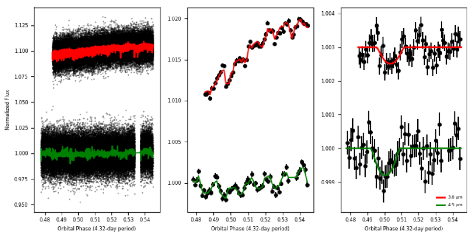
Figure 1: Individually-fit BLISS light curves of WASP-34. The 3.6 µm observation has been vertically offset for visual clarity. Note that we clipped out frames 49000 – 52000 due to erratic sky levels and frames 53740 – 53790 due to a reaction wheel spike. Left: Normalized raw photometry with best-fit models overplotted. Middle: Normalized binned photometry and binned best-fit models. Right: Normalized binned photometry and best-fit models with systematics divided out to highlight the eclipses.

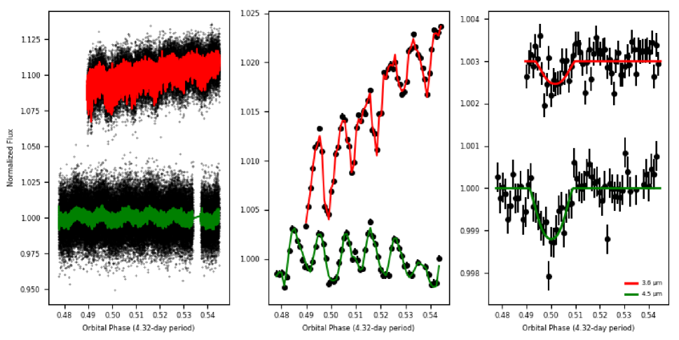
Figure 2: Individually-fit PLD light curves of WASP-34. The 3.6 µm observation has been vertically offset for visual clarity. Note that we clipped out frames 49000 – 52000 due to erratic sky levels and frames 53740 – 53790 due to a reaction wheel spike. Left: Normalized raw photometry with best-fit models overplotted. Middle: Normalized binned photometry and binned best-fit models. Right: Normalized binned photometry and best-fit models with systematics divided out to highlight the eclipses.

The binned light curves show some potential residual correlated noise. While our light-curve optimization methods minimize correlated noise, we compare the residual RMS vs. different bin sizes with the expected standard error in Figure 3. There is some correlated noise present, but it is within 1$\sigma$ of the expected standard error at nearly all bin sizes.

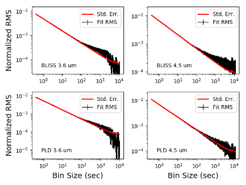
Figure 3: Comparison of fit residual RMS vs. bin size with the expected standard error. If the fit residual RMS is above the standard error, there is correlated noise present at that time scale. For all four cases, the standard error is within the uncertainties of the residual fit RMS at nearly all bin sizes, indicating low residual correlated noise.

3.2 4.5 µm

Since the planet is brighter at 4.5 µm than 3.6 µm relative to the host star, here we expect a deeper eclipse. Indeed, BLISS finds an eclipse depth of $895\pm 201$ at $2455405.30880\pm 0.00327$ $\textrm{BJD}_{\textrm{TDB}}$, and PLD finds an eclipse depth of $1312\pm 147$ ppm at $2455405.30727\pm 0.00253$ $\textrm{BJD}_{\textrm{TDB}}$, using a bin size of 16 frames. These depths correspond to band-integrated brightness temperatures of $1279\pm 103$ K and $1475\pm 67$ K for BLISS and PLD, respectively. Figures 1 and 2 show the BLISS and PLD fits. Due to unusual sky level activity and a reaction wheel spike, we removed frames 49000 – 52000 and 53740 – 53790, respectively. Again, Table 2 compares the ramp models and Figure 3 checks for residual correlated noise.

We note there is a $\sim$1.7$\sigma$ difference between these eclipse depths. This is entirely due to differences in the selected photometry methods. Regardless of PLD or BLISS, fixed aperture photometry finds an eclipse depth of $\sim$850 ppm, whereas variable and elliptical photometry produce an eclipse depth of $\sim$1300 ppm. Since the $\chi^{2}_{\textrm{bin}}$ prefers elliptical photometry when using a PLD model, we present those results, but note that, at least in this observation, the choice of photometry method impacts results.

4 Joint Light-Curve Modeling

In an attempt to further constrain $b$, eclipse midpoint, and planet-to-star flux ratio, we jointly fit to both light curves, with both BLISS and PLD using the photometry listed in Table 1. We use the same model parameterization scheme as described above, but share $b$, $P$, $R_{s}$, $R_{p}$, $a$, and eclipse midpoint (in orbital-phase space) between models of the 3.6 µm and 4.5 µm eclipses. With BLISS, we find $b=0.907\pm 0.016$, 3.6 µm eclipse depth of $455\pm 165$ pmm (1191 $\pm$ 129 K), 4.5 µm eclipse depth of $868\pm 196$ ppm (1261 $\pm$ 105 K), and an eclipse midpoint of $0.5018\pm 0.0007$ orbital phase. Using the same configuration with PLD, we find $b=0.907\pm 0.015$, a 3.6 µm eclipse depth of $606\pm 147$ ppm (1299 $\pm$ 98 K), a 4.5 µm eclipse depth of $1283\pm 310$ ppm (1463 $\pm$ 127 K), and an eclipse midpoint of $0.5012\pm 0.0006$ orbital phase. The joint-fit eclipse midpoints are consistent with the individual fits within $1.4\sigma$, and the eclipse depths are consistent within $0.5\sigma$.

5 Orbit

Eclipse observations, since they sample a different portion of the orbit than transits, can significantly reduce uncertainties on eccentricity, as well as detect eccentricity false positives in radial-velocity (RV) data (Arras et al. 2012). We used RadVel (Fulton et al. 2018) to fit a Keplerian orbit to the measured eclipse midpoint timings, published and amateur transit ephemerides (var2.astro.cz/ETD/, Table 3), and RV data (Table 4). None of the RV data occur during transit, so there is no need to account for the Rossiter-McLaughlin effect.

Table 3: WASP-34b Transit Observations

Time	Uncertainty	Reference
(BJD${}_{\textrm{TDB}}$)	(BJD${}_{\textrm{TDB}}$)
2455739.92619	0.00117	ETD: Curtis I.
2455726.97299	0.0016	ETD: Curtis I.
2455631.97466	0.0013	ETD: Evans P.
2455580.17290	0.00116	ETD: Tan TG
2454647.55359	0.00064	Smalley et al. (2011)

Table 4: WASP-34b Radial Velocity Data

Time	RV	Reference
(BJD${}_{\textrm{TDB}}$)	(m/s)
2455166.8246	49790.3 $\pm$ 4.4	1
2455168.8191	49937.2 $\pm$ 4.3	1
2455170.8439	49792.3 $\pm$ 4.2	1
2455172.8246	49925.3 $\pm$ 4.6	1
2455174.8495	49814.1 $\pm$ 4.1	1
2455175.8487	49797.3 $\pm$ 3.9	1
2455176.8235	49880.6 $\pm$ 4.2	1
2455179.8425	49788.8 $\pm$ 4.1	1
2455180.8566	49861.1 $\pm$ 4.1	1
2455181.8219	49941.4 $\pm$ 4.2	1
2455182.8521	49876.5 $\pm$ 4.9	1
2455184.8554	49843.2 $\pm$ 4.4	1
2455186.8299	49905.8 $\pm$ 4.6	1
2455190.8509	49915.2 $\pm$ 4.5	1
2455261.7740	49768.6 $\pm$ 4.9	1
2455262.6724	49819.1 $\pm$ 4.1	1
2455372.5078	49873.1 $\pm$ 5.0	1
2455375.6020	49879.7 $\pm$ 7.0	1
2455376.5170	49895.6 $\pm$ 8.0	1
2455380.5170	49892.2 $\pm$ 4.8	1
2455391.4971	49763.1 $\pm$ 5.3	1
2455399.4719	49769.5 $\pm$ 4.8	1
2455403.4683	49815.9 $\pm$ 4.9	1
2455410.4719	49891.3 $\pm$ 4.9	1
2455902.1333619	-29.089 $\pm$ 1.561	2
2455903.0804119	6.179 $\pm$ 1.576	2
2455904.1423798	-80.603 $\pm$ 1.542	2
2455932.1205709	-54.071 $\pm$ 1.664	2
2456266.1084835	57.445 $\pm$ 1.547	2
2456320.1059713	-27.768 $\pm$ 2.146	2
2456326.1395332	90.815 $\pm$ 2.212	2
2456639.1639846	37.544 $\pm$ 1.684	2

From long-term trends in the RV data, there is a candidate large-orbit companion in the system (Smalley et al. 2011, Knutson et al. 2014). We include this object to accurately model the RV data, although the new data in this work place no additional constraints on the companion. Our model includes terms for $e\textrm{cos}\omega$, $e\textrm{sin}\omega$, transit ephemeris $T_{0}$, orbital period, RV semi-amplitude $K$, RV zero point $\gamma$ (per instrument), and RV jitter $j$ (per instrument). Like Knutson et al. (2014), we set $e\textrm{cos}\omega$ and $e\textrm{sin}\omega$ of the companion to 0.

We fit to both the BLISS and PLD results (individual fits from Sections 3.1 and 3.2, since using the joint fits would force a conversion from orbital phase space to a single Julian date, but the joint fit encompasses two eclipses) to check for consistency (see Table 5). The two fits agree well on all orbital parameters except $e_{b}\textrm{cos}\omega_{b}$, which differs by 1.7$\sigma$. However, the uncertainty on the derived $e$ is driven by the larger uncertainty on $e_{b}\sin\omega_{b}$, so there is an insignificant difference in the recovered planetary eccentricity. The addition of amateur transit timings and the eclipses from this work improves the uncertainty on orbital period by 13% over Knutson et al. (2014).

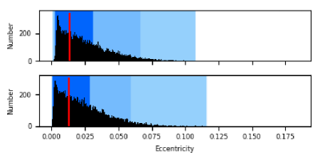
Figure 4: Eccentricity histograms derived from MCMC posterior distributions of $e\textrm{sin}\omega$ and $e\textrm{cos}\omega$. The red line marks the best-fit value, and the blue regions denote the 1, 2, and 3$\sigma$ regions. Top: Posterior from the fit to the BLISS results. Bottom: Posterior from the fit to the PLD results.

The 1$\sigma$ uncertainty on $e$ indicates only a marginal detection of eccentricity, consistent with Knutson et al. (2014) and Bonomo et al. (2017). However, the posterior distributions show a 2–3$\sigma$ detection so we investigate the expected circularization timescale for this planet and compare with the age of the system. This timescale, from Goldreich & Soter (1966), is given by

$$\tau_{e}=\frac{4}{63}Q\left(\frac{a^{3}}{GM}\right)^{1/2}\left(\frac{m}{M}\right)\left(\frac{a}{R_{\textrm{p}}}\right)^{5},$$ (19)

where Q is a tidal dissipation factor, typically $\sim 10^{6}$ for hot Jupiters (Wu 2005), $a$ is orbital radius, $M$ is stellar mass, $m$ is planetary mass, and $R_{p}$ is planetary radius. Using $M=1.01\ M_{\odot}$, $m=0.59\ R_{\textrm{J}}$, and $a=0.0524$ AU (Smalley et al. 2011), we determine a circularization timescale of $\sim$ 4$\times 10^{8}$ years. Smalley et al. (2011) note that lithium depletion in WASP-34 indicates an age $\gtrsim$ 5 Gyr (Sestito & Randich 2005), implying that the planet’s orbit should have circularized. This is consistent with our results within $\sim 2\sigma$.

Table 5: WASP-34b Orbital Parameters

	BLISS	PLD	Knutson et al. (2014)
Fitted Parameters
$e_{b}$ sin $\omega_{b}$	-0.013 $\pm$ 0.029	-0.013 $\pm$ 0.028	-0.001${}^{+0.011}_{-0.017}$
$e_{b}$ cos $\omega_{b}$	0.0036 $\pm$ 0.0009	0.0016 $\pm$ 0.0008	-0.0001${}^{+0.0068}_{-0.0071}$
$P_{b}$ (days)	4.3176694 $\pm$ 0.0000038	4.3176694 $\pm$ 0.0000039	4.3176779 $\pm$ 0.0000045
$T_{0,b}$ (BJD${}_{\textrm{TDB}}$)	2454647.55357 $\pm$ 0.00065	2454647.55357 $\pm$ 0.00065	2454647.55434${}^{+0.00063}_{-0.00064}$
$K_{b}$ (m/s)	71.0 $\pm$ 1.7	71.0 $\pm$ 1.7	71.1${}^{+1.6}_{-1.7}$
$e_{c}$ sin $\omega_{c}$	0	0	0
$e_{c}$ cos $\omega_{c}$	0	0	0
$P_{c}$ (days)	3990 $\pm$ 810	3960 $\pm$ 760	4093${}^{+750}_{-520}$
$T_{0,c}$ (BJD${}_{\textrm{TDB}}$)	2454612 $\pm$ 210	2454618 $\pm$ 200	2454589${}^{+140}_{-190}$
$K_{c}$ (m/s)	180 $\pm$ 60	179 $\pm$ 54	189${}^{+60}_{-35}$
$\gamma_{\rm CORALIE}$ (m/s)	50000 $\pm$ 62	49999 $\pm$ 57	141${}^{+62}_{-37}$
$\gamma_{\rm HIRES}$ (m/s)	99 $\pm$ 62	97 $\pm$ 56	108${}^{+62}_{-37}$
$j_{\rm CORALIE}$ (m/s)	6.1 $\pm$ 1.7	6.1 $\pm$ 1.7	—
$j_{\rm HIRES}$ (m/s)	1.7 $\pm$ 4.6	1.5 $\pm$ 4.2	—
$j$ (m/s)	—	—	3.2${}^{+0.72}_{-0.6}$
Derived Parameters
$e_{b}$	0.014${}^{+0.017}_{-0.010}$	0.013${}^{+0.015}_{-0.012}$	0.0109${}^{+0.015}_{-0.0078}$
$\omega_{b}$ (°)	286 $\pm$ 80	277 $\pm$ 86	215${}^{+77}_{-140}$
$e_{c}$	0	0	0
$\omega_{c}$ (°)	0	0	0

6 Atmosphere

We used our Bayesian Atmospheric Radiative Transfer code (BART, Harrington et al. 2021, Cubillos et al. 2021, Blecic et al. 2021) to retrieve the atmosphere of WASP-34b. BART consists of three main packages: Transit (Rojo 2006), a radiative transfer code that produces spectra from a parameterized atmosphere model; Thermochemical Equilibrium Abundances (TEA, Blecic et al. 2016), which calculates species abundances at each pressure and temperature in a planet’s atmosphere based on equilibrium chemistry; and MC³ (Cubillos et al. 2017), an MCMC routine wrapper. BART ties these packages together to retrieve thermal profiles and abundances of atmospheric constituents from eclipse or transit observations.

BART parameterizes the planetary thermal structure with the thermal profile from Line et al. (2013). This model has five free parameters: $\kappa$, the infrared Planck mean opacity; $\gamma_{1}$ and $\gamma_{2}$, the ratios of Planck mean opacities in the two visible streams to the infrared stream; $\alpha$, which splits flux between the two visible streams; and $\beta$, which covers albedo, emissivity, and heat redistribution. We also fit logarithmic scale factors on the abundances of H₂O, CH₄, CO, and CO₂. All parameter ranges are wide, and priors are uniform. Given the low signal-to-noise of our data and the limited spectral coverage, we use uniform abundances with respect to pressure. We include opacity from the four aforementioned molecules (Rothman et al. 2010, Li et al. 2015, Hargreaves et al. 2020) as well as H₂ - H₂ collision-induced absorption.

Our spectrum is only two broadband photometric filters, so models are prone to overfitting. We try several statistically- and physically-motivated cases to determine what information we can learn from our data:

1. All parameters free ($\kappa$, $\gamma_{1}$, $\gamma_{2}$, $\alpha$, $\beta$, and logarithmic scale factors for H₂O, CH₄, CO, and CO₂ abundances).

2. Since methane and CO₂ are not expected to be abundant at the equilibrium temperature of WASP-34b, we fix their abundances to 6.93$\times 10^{-6}$ and 1.66$\times 10^{-7}$, respectively. These are TEA-computed values at 0.1 bars pressure and the planetary equilibrium temperature of 1158 K, assuming 0 albedo and uniform heat redistribution. Thermal profile parameters and the other molecular abundances are left free to vary.

3. Same as 2, but the the CO mixing ratio is fixed to 4.53$\times 10^{-4}$ (thermochemical equilibrium as in case 2), since only the 4.5 µm filter is sensitive to CO abundance.

4. Same as 3, but the H₂O mixing ratio is fixed to 3.84$\times 10^{-6}$ (thermochemical equilibrium as in case 2). Only the thermal profile parameters are free to vary.

5. Same as 4, but $\alpha=0.0$ and $\gamma_{2}=1$, removing one visible stream.

6. Same as 5, but $\beta=1$. This sets the irradiation temperature equal to the planet’s equilibrium temperature, assuming zero albedo and perfect heat redistribution.

7. An isothermal atmosphere, where planetary temperature is the only free parameter.

Case 1 represents the most flexible model, cases 2 – 4 make simplifying assumptions about the atmospheric composition, and cases 5 – 7 represent a range from complex to simple thermal profiles, all with vertically-uniform molecular abundances. All cases include the same opacity sources. As with the “ramp” in the light-curve modeling, we use the BIC to determine which model is warranted by our data (Equation 11, Table 6). We fit to both the PLD and BLISS eclipse depths, separately, to compare results, using the joint fits (Section 4), as the shared parameters should lead to more accurate uncertainties.

Table 6: Atmospheric Fit BICs

	BLISS		PLD
Case	BIC	$P_{21}$	BIC	$P_{21}$
1	6.2384	0.0635	6.2387	0.0795
2	4.8523	0.1270	4.8542	0.1589
3	4.1590	0.1796	4.1591	0.2249
4	3.4661	0.2540	3.5001	0.3127
5	2.0800	0.5079	2.2010	0.5988
6	1.3878	0.7180	1.5291	0.8379
7	0.7251	—	1.1753	—

The retrievals using the PLD and BLISS eclipse depths are very similar. Cases 1, 2, and 3 result in fits with unconstained abundances for all fitted molecules, with flat MCMC posteriors, indicating that for any abundance within reasonable parameter bounds, there exists a parameter set that fits equally well. The flat posteriors and a BIC comparison show we are statistically justified in fixing the molecular abundances to thermochemical equilibrium (Table 6). Likewise, our data are unable to support a temperature structure as complex as case 4, with an uninformative posterior distribution for $\alpha$. Cases 5, 6, and 7 have informative (non-flat) marginalized posterior distributions for their parameters, although cases 5 and 6 still overfit the data. With both the BLISS and PLD eclipse depths, we find we are only justified in fitting an isothermal atmosphere. We determine an isothermal temperature of 1093 $\pm$ 66 K with BLISS (Figure 5, left) and 1194 $\pm$ 66 K with PLD (Figure 5, right).

We tested MCMC convergence by ensuring that the Gelman & Rubin test was within 1% of unity for all free parameters (Gelman & Rubin 1992). Also, we computed the Steps Per Effectively Independent Sample and Effective Sample Size (SPEIS, ESS, Harrington et al. 2021) to verify that the posterior distribution is well explored. Using the BLISS observations, we find a SPEIS of 10, an ESS of 400, and a $68.3\pm 2.3$% ($1\sigma$) credible region of [1026, 1159] K for the isothermal planet temperature. For the PLD observations, we find a SPEIS of 10, an ESS of 500, and a $68.3\pm 2.1$% credible region of [1130, 1263] K for the isothermal planet temperature.

Per the BART license, the code version, inputs, outputs, and output-processing scripts for these best-fitting atmospheres, with step-by-step instructions to reproduce the results presented in this work, are contained in a reproducible-research compendium which can be found on Zenodo doi:10.5281/zenodo.5096510. The compendium also includes the light-curve data, models, and diagnostic plots.

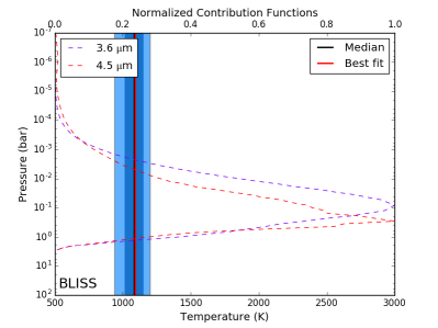
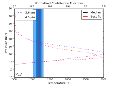
Figure 5: Lowest BIC BART-retrieved temperature-pressure profiles. Dark blue and light blue regions denote the 1 and 2$\sigma$ boundaries, respectively. We have overplotted contribution functions for the two Spitzer data points, which show the portion of the atmosphere probed by our retrieval. Left: The isothermal (case 7) profile retrieved from the BLISS eclipse depths. Right: The thermal profile retrieved using PLD eclipse depths (case 6).

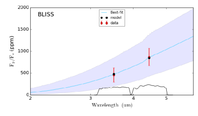
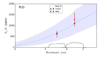
Figure 6: Lowest BIC BART-retrieved spectra as planet-to-star flux ratio. The black dots are the spectrum integrated over the filters. The black dots, not the light blue line, should match the red data. The shaded region denotes the 3$\sigma$ uncertainty on the best-fit isothermal atmosphere. The IRAC response functions are plotted along the $y$ axis (arbitrary units). Left: Isothermal (blackbody) spectrum retrieved using the BLISS eclipse depths. Features are caused by the stellar spectrum (ATLAS9, Castelli & Kurucz 2004); the planetary spectrum is a smooth blackbody curve. Right: The isothermal spectrum retrieved using the PLD eclispe depths.

7 Discussion

With the number of Jupiters with measured emission increasing, many studies have taken a statistical approach to exoplanet atmospheres, both in transmission (e.g., Baxter et al. 2021) and emission (e.g., Garhart et al. 2020, Wallack et al. 2021). Here we compare WASP-34b against the literature of comparative exoplanetology to study how it fits into observed trends.

Garhart et al. (2020) noted a trend with slope 0.00043 $\pm$ 0.000072 in eclipse phase shift from a circular orbit vs. orbital period. At WASP-34b’s orbital period, we would expect a shift of 0.00186 $\pm$ 0.00031 orbital phase. From joint light-curve fits, we determined the eclipse phase shift to be 0.0018 $\pm$ 0.0007 (BLISS) and 0.0012 $\pm$ 0.0006 (PLD). The circularization of WASP-34b agrees well with this trend.

Several studies have looked into trends in the ratio of 4.5 to 3.6 µm brightness temperatures (Kammer et al. 2015, Wallack et al. 2019, Garhart et al. 2020, Wallack et al. 2021). From our joint light-curve fits we measured brightness temperature ratios of 1.05 $\pm$ 0.14 (BLISS) and 1.13 $\pm$ 0.12 (PLD). WASP-34b may have a larger brightness temperature ratio than other planets with a similar equilibrium temperature, which generally fall below 1.0 (e.g., WASP-6b, WASP-8b, WASP-39b, TrES-1b, Wallack et al. 2021), although the weak eclipses lead to large uncertainties. WASP-34b may exhibit different chemistry than other warm Jupiters at the pressures probed by these observations. For instance, 4.5 µm CO emission or 3.6 µm CH₄ absorption could cause a redder slope. The planet’s unusual color is not attributable to its surface gravity (log($g$) = 3.0) or host star metalliticy ([Fe/H] = -0.02 $\pm$ 0.10, Smalley et al. 2011), as these values are similar to other warm Jupiters observed with Spitzer.

8 Conclusions

We analyzed two Spitzer observations of the exoplanet WASP-34b using two light-curve modeling methods, BLISS and PLD, and applying a modified eclipse model to account for the planet’s high impact parameter, demonstrating observational feasibility for low-signal, grazing eclipses. The resulting eclipse depths, from joint fits to both light curves, agree at $\leq 1.1\sigma$ and eclipse midpoint agrees at $0.7\sigma$ between the two methods. By minimizing a combination of white and correlated noise, BLISS selects a fixed photometry aperture radius but PLD prefers a variable aperture radius. If the two models are forced to use the same light curve, the resulting eclipse depths more closely match.

The measured eclipse midpoints further constrained the orbit of the planet. We determined an eccentricity consistent with zero (0.0), similar to previous works (Knutson et al. 2014, Bonomo et al. 2017). While $e\textrm{cos}\omega$ differs by $1.7\sigma$ between fits to the BLISS and PLD eclipses, all other fitted and derived orbital parameters are consistent between the two orbital fits.

We also performed atmospheric retrieval on our measured eclipse depths, separately for each light-curve modeling technique, using a series of physically-motivated cases to determine what we could learn from the data. For both BLISS and PLD, despite differences in the eclipse depths, we preferred atmopsheric models that fixed molecular abundances to thermochecmical equilibrium over those that fit the abundances. Thus, we cannot constrain atmospheric constituents. We find the best model, by BIC comparison, is an isothermal atmosphere at $\sim$1100 – 1200 K.

WASP-34b is somewhat unusual, with its density among the lowest 0.8% of planets with a measured radius and mass. The planet is redder than other Jupiters with this equilibrium temperature, possibly indicating unique chemistry, and the large scale height implied by its low density makes it an attractive target for transit studies. Unfortunately, the planet’s grazing nature makes it difficult to observe and characterize. Further improvement over the atmospheric results presented here may be posssible with the Hubble Space Telescope, at least in transit geometry, but additional eclipses to constrain the dayside atmosphere and orbit likely must wait for the James Webb Space Telescope.

9 Acknowledgements

We thank the referees for their insightful comments and the resulting improvements to this manscript. We thank contributors to SciPy, Matplotlib, and the Python Programming Language, the free and open-source community, the NASA Astrophysics Data System, and the JPL Solar System Dynamics group for software and services. This work is based on observations made with the Spitzer Space Telescope, which was operated by the Jet Propulsion Laboratory, California Institute of Technology under a contract with NASA. This work was supported by NASA Planetary Atmospheres grant NNX12AI69G and NASA Astrophysics Data Analysis Program grant NNX13AF38G. Jasmina Blecic is supported by NASA through the NASA ROSES-2016/Exoplanets Research Program, grant NNX17AC03G.

Spitzer (IRAC)

References

- Arras et al. (2012) Arras, P., Burkart, J., Quataert, E., & Weinberg, N. N. 2012, MNRAS, 422, 1761, doi: 10.1111/j.1365-2966.2012.20756.x
- Baxter et al. (2021) Baxter, C., Désert, J.-M., Tsai, S.-M., et al. 2021, A&A, 648, A127, doi: 10.1051/0004-6361/202039708
- Blecic et al. (2016) Blecic, J., Harrington, J., & Bowman, M. O. 2016, ApJS, 225, 4, doi: 10.3847/0067-0049/225/1/4
- Blecic et al. (2013) Blecic, J., Harrington, J., Madhusudhan, N., et al. 2013, ApJ, 779, 5, doi: 10.1088/0004-637X/779/1/5
- Blecic et al. (2014) —. 2014, ApJ, 781, 116, doi: 10.1088/0004-637X/781/2/116
- Blecic et al. (2021) Blecic, J., Harrington, J., Cubillos, P., et al. 2021, in review
- Bonomo et al. (2017) Bonomo, A. S., Desidera, S., Benatti, S., et al. 2017, A&A, 602, A107, doi: 10.1051/0004-6361/201629882
- Castelli & Kurucz (2004) Castelli, F., & Kurucz, R. L. 2004, ArXiv Astrophysics e-prints
- Challener et al. (2021) Challener, R. C., Harrington, J., Jenkins, J., et al. 2021, The Planetary Science Journal, 2, 9, doi: 10.3847/PSJ/abc954
- Charbonneau et al. (2005) Charbonneau, D., Allen, L. E., Megeath, S. T., et al. 2005, ApJ, 626, 523, doi: 10.1086/429991
- Cubillos et al. (2017) Cubillos, P., Harrington, J., Loredo, T. J., et al. 2017, AJ, 153, 3, doi: 10.3847/1538-3881/153/1/3
- Cubillos et al. (2014) Cubillos, P., Harrington, J., Madhusudhan, N., et al. 2014, ApJ, 797, 42, doi: 10.1088/0004-637X/797/1/42
- Cubillos et al. (2013) —. 2013, ApJ, 768, 42, doi: 10.1088/0004-637X/768/1/42
- Cubillos et al. (2021) Cubillos, P., Harrington, J., Blecic, J., et al. 2021, in review
- Deming et al. (2015) Deming, D., Knutson, H., Kammer, J., et al. 2015, ApJ, 805, 132, doi: 10.1088/0004-637X/805/2/132
- Fazio et al. (2004) Fazio, G. G., Hora, J. L., Allen, L. E., et al. 2004, ApJS, 154, 10, doi: 10.1086/422843
- Fulton et al. (2018) Fulton, B. J., Petigura, E. A., Blunt, S., & Sinukoff, E. 2018, PASP, 130, 044504, doi: 10.1088/1538-3873/aaaaa8
- Garhart et al. (2020) Garhart, E., Deming, D., Mandell, A., et al. 2020, AJ, 159, 137, doi: 10.3847/1538-3881/ab6cff
- Gelman & Rubin (1992) Gelman, A., & Rubin, D. B. 1992, Statistical Science, 7, 457, doi: 10.1214/ss/1177011136
- Gibson et al. (2012) Gibson, N. P., Aigrain, S., Roberts, S., et al. 2012, MNRAS, 419, 2683, doi: 10.1111/j.1365-2966.2011.19915.x
- Goldreich & Soter (1966) Goldreich, P., & Soter, S. 1966, Icarus, 5, 375, doi: 10.1016/0019-1035(66)90051-0
- Hardy et al. (2017) Hardy, R. A., Harrington, J., Hardin, M. R., et al. 2017, ApJ, 836, 143, doi: 10.3847/1538-4357/836/1/143
- Hargreaves et al. (2020) Hargreaves, R. J., Gordon, I. E., Rey, M., et al. 2020, ApJS, 247, 55, doi: 10.3847/1538-4365/ab7a1a
- Harrington et al. (2021) Harrington, J., Himes, M., Cubillos, P., et al. 2021, in review
- Harris et al. (2020) Harris, C. R., Jarrod Millman, K., van der Walt, S. J., et al. 2020, Nature, 585, 357, doi: 10.1038/s41586-020-2649-2
- Hunter (2007) Hunter, J. D. 2007, Computing in Science & Engineering, 9, 90, doi: 10.1109/MCSE.2007.55
- Ingalls et al. (2016) Ingalls, J. G., Krick, J. E., Carey, S. J., et al. 2016, AJ, 152, 44, doi: 10.3847/0004-6256/152/2/44
- Kammer et al. (2015) Kammer, J. A., Knutson, H. A., Line, M. R., et al. 2015, ApJ, 810, 118, doi: 10.1088/0004-637X/810/2/118
- Knutson et al. (2014) Knutson, H. A., Fulton, B. J., Montet, B. T., et al. 2014, ApJ, 785, 126, doi: 10.1088/0004-637X/785/2/126
- Lewis et al. (2013) Lewis, N. K., Knutson, H. A., Showman, A. P., et al. 2013, ApJ, 766, 95, doi: 10.1088/0004-637X/766/2/95
- Li et al. (2015) Li, G., Gordon, I. E., Rothman, L. S., et al. 2015, ApJS, 216, 15, doi: 10.1088/0067-0049/216/1/15
- Line et al. (2013) Line, M. R., Wolf, A. S., Zhang, X., et al. 2013, ApJ, 775, 137, doi: 10.1088/0004-637X/775/2/137
- Lust et al. (2014) Lust, N. B., Britt, D., Harrington, J., et al. 2014, PASP, 126, 1092, doi: 10.1086/679470
- Mandel & Agol (2002) Mandel, K., & Agol, E. 2002, ApJ, 580, L171, doi: 10.1086/345520
- Morello et al. (2015) Morello, G., Waldmann, I. P., Tinetti, G., et al. 2015, ApJ, 802, 117, doi: 10.1088/0004-637X/802/2/117
- Nymeyer et al. (2011) Nymeyer, S., Harrington, J., Hardy, R. A., et al. 2011, ApJ, 742, 35, doi: 10.1088/0004-637X/742/1/35
- Raftery (1995) Raftery, A. E. 1995, Sociological Mehodology, 25, 111
- Rojo (2006) Rojo, P. M. 2006, PhD thesis, Cornell University
- Rothman et al. (2010) Rothman, L. S., Gordon, I. E., Barber, R. J., et al. 2010, J. Quant. Spec. Radiat. Transf., 111, 2139, doi: 10.1016/j.jqsrt.2010.05.001
- Sestito & Randich (2005) Sestito, P., & Randich, S. 2005, A&A, 442, 615, doi: 10.1051/0004-6361:20053482
- Smalley et al. (2011) Smalley, B., Anderson, D. R., Collier Cameron, A., et al. 2011, A&A, 526, A130, doi: 10.1051/0004-6361/201015992
- Stevenson et al. (2012) Stevenson, K. B., Harrington, J., Fortney, J. J., et al. 2012, ApJ, 754, 136, doi: 10.1088/0004-637X/754/2/136
- Virtanen et al. (2020) Virtanen, P., Gommers, R., Oliphant, T. E., et al. 2020, Nature Methods, 17, 261, doi: 10.1038/s41592-019-0686-2
- Wallack et al. (2021) Wallack, N. L., Knutson, H. A., & Deming, D. 2021, arXiv e-prints, arXiv:2103.15833. https://arxiv.org/abs/2103.15833
- Wallack et al. (2019) Wallack, N. L., Knutson, H. A., Morley, C. V., et al. 2019, AJ, 158, 217, doi: 10.3847/1538-3881/ab2a05
- Werner et al. (2004) Werner, M. W., Roellig, T. L., Low, F. J., et al. 2004, ApJS, 154, 1, doi: 10.1086/422992
- Wu (2005) Wu, Y. 2005, ApJ, 635, 688, doi: 10.1086/497355