Plotting in a Formally Verified Way

Abstract

An invaluable feature of computer algebra systems is their ability to plot the graph of functions. Unfortunately, when one is trying to design a library of mathematical functions, this feature often falls short, producing incorrect and potentially misleading plots, due to accuracy issues inherent to this use case. This paper investigates what it means for a plot to be correct and how to formally verify this property. The Coq proof assistant is then turned into a tool for plotting function graphs using reliable polynomial approximations. This feature is provided as part of the CoqInterval library.

1 Introduction

An invaluable feature of computer algebra systems (Maple, Mathematica, etc) is their ability to plot the graph of mathematical functions. Indeed, as the adage goes, a picture is worth a thousand words. When encountering an unknown function, the first reflex of the user is to plot it, so as to grasp its features. But how much can the user trust that the plot is an accurate depiction of the graph of the function?

Let us consider the case of a user who wants to implement a floating-point library of mathematical functions. The implementation of such a function, e.g., $\exp$, usually involves some polynomial $p$, since processors are efficient at addition and multiplication. The distance $|p(x)-\exp x|$ characterizes the quality of the approximation and thus of the implementation. So, one might be tempted to plot $p(x)-\exp x$ and look at its extrema. Let us assume that $p$ is the minimax approximation of degree 6 between $-2^{-5}$ and $2^{-5}$ with binary64 floating-point coefficients. Figure 1(a) shows what the signed distance looks like, when plotted with Gnuplot. The result certainly looks questionable, and other computer algebra systems would hardly do better.

The main issue is that these systems plot the function graph using plain binary64 arithmetic, which is way too inaccurate for our use case. The Sollya tool was especially designed to solve this kind of issue [2]. By using a 165-bit arithmetic, it is able to produce Figure 1(c), which is representative of what the distance between a function and its minimax polynomial usually looks like (cf. La Vallée-Poussin’s theorem). The user can now look at the plotted function graph and see that the distance is bounded by $10^{-16}$, which might be sufficient, depending on the purpose of the mathematical library.

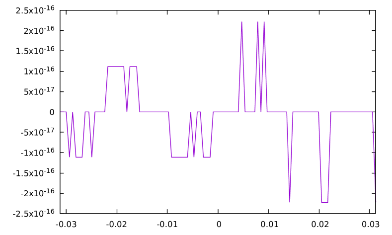
(a) Gnuplot

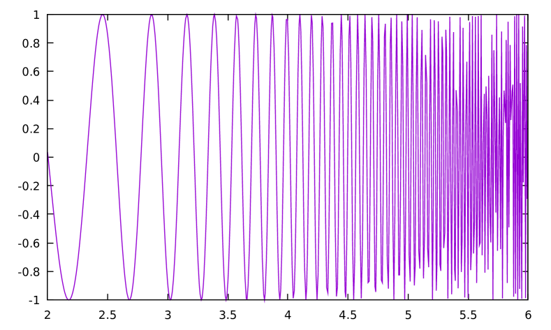
(b) Sollya

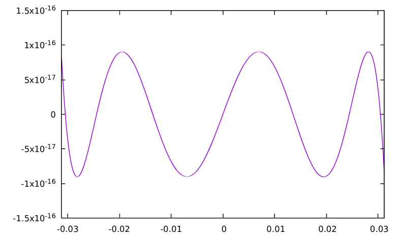
(c) Sollya and this work

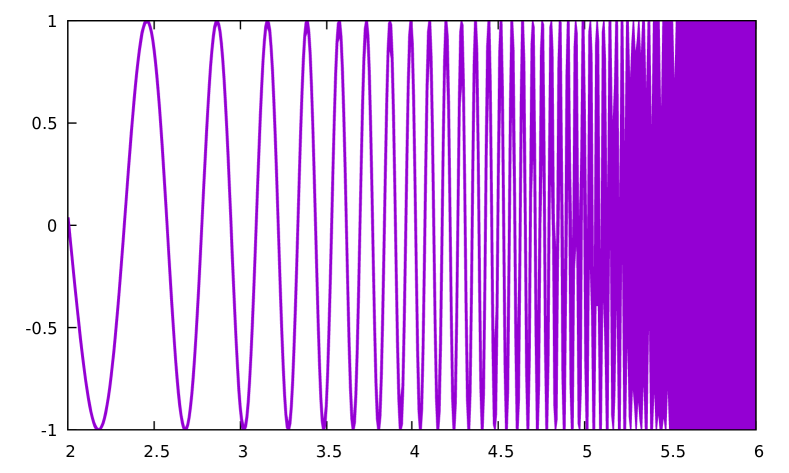
(d) This work

Figure 1: On the left, distance between $\exp$ and its minimax. On the right, $x\to\sin(x+\exp x)$.

But what if the function graph needs more than 165 bits of precision to be plotted correctly? Sollya actually performs its computations using interval arithmetic. Instead of computing a single floating-point number that approximates the real value of the function, it computes two floating-point bounds that enclose this real value. So, by looking at the distance between these bounds, it is able to detect when its internal precision is not sufficient for a correct plot. In that case, the user can increase the precision.

So, did Sollya actually solve the issue of plotting? Not quite. As other computer algebra systems, it heuristically samples the plotted function. So, any feature of the function that occurs between two sampled abscissas will not appear on the plot. Consider the function $f(x)=\sin(x+\exp x)$. This time, there is no precision issue; even binary32 floating-point arithmetic could be used. But the function oscillates so quickly that the plot is not faithful, as shown on Figure 1(b). For $x\geq 4$, the function does not even seem to reach $-1$ and $1$ anymore, although it is the sine function.

Let us define a correct plot as follows: If a pixel is blank, then there exists no value of $x$ such that $(x,f(x))$ falls into this pixel. Conversely, a complete plot is defined as follows: If a pixel is filled, then there exists a value of $x$ such that $(x,f(x))$ falls into it. This article explains how one can draw correct plots, as shown on Figures 1(c) and 1(d). To increase the confidence in the plots, they are performed using the Coq system. This is not the first work to explore the topic of correct (and complete) plots using a proof assistant [6], but this works focuses on producing plots in a matter of seconds rather than hours.

Section 2 explains how to formally define what a correct plot is. Section 3 then shows how to compute it inside the logic of Coq, using the CoqInterval library [5]. It also explains how to get close to a complete plot. Coq gives the greatest confidence in the correctness of the plots, but it hardly strikes as a user-friendly system when it comes to computer algebra. So, Section 4 focuses on interface concerns.

2 Formal Specification

The very first step is to state what it means for a plot to be correct. We have some function $f$ from real numbers to real numbers. Note that this is a function defined in a purely mathematical sense; no floating-point numbers are involved here. We also have some bounds $x_{\_}1$ and $x_{\_}2$ between which we will plot the function graph. Again, these are real numbers. We will not use them directly though, as it makes for much more readable (and thus trustable) definitions to use two real numbers $\mathit{ox}$ and $\mathit{dx}$ such that $x_{\_}1=\mathit{ox}$ and $x_{\_}2=\mathit{ox}+\mathit{dx}\cdot w$. In other words, if the output device has an horizontal resolution of $w$ pixels, then $\mathit{dx}$ will be the width of a single pixel, while $\mathit{ox}$ will point at the left border of the leftmost pixel.

A plot will then be defined as a list $\ell$ of intervals. The $i$-th interval $\ell_{\_}i$ encloses all the possible values of the function for the $i$-th pixel:

$$\forall x,~{}\mathit{ox}+\mathit{dx}\cdot i\leq x\leq\mathit{ox}+\mathit{dx}\cdot(i+1)\Rightarrow f(x)\in\ell_{\_}i.$$

The translation to Coq is straightforward (with I a module containing interval-related definitions):

⬇

Definition plot1 (f:R->R) (ox dx:R) (l:list I.type) :=

forall (i:nat) (x:R), ox + dx * i <= x <= ox + dx * (i + 1) ->

I.contains (nth i l I.nai) (f x).

The interval I.nai, which contains any real number, is the default value used when the list $\ell$ is exhausted. Thus, the predicate plot1 is still valid when $i$ exceeds the length of $\ell$. In particular, if this length is smaller than $w$, the rightmost part of the plot will be entirely comprised of filled pixels.

This could be the end of it, but since I.type is an internal datatype, it might be difficult to turn the list into a bitmap or to serialize it to another tool. So, in order to use a more universal datatype, namely integers of type Z, a second predicate is defined. To do so, we need two more real numbers: $\mathit{oy}$ and $\mathit{dy}$. They play a role similar to $\mathit{ox}$ and $\mathit{dx}$, but along the vertical axis:

⬇

Definition plot2 (f:R->R) (ox dx oy dy:R) (h:Z) (l:list (Z*Z)) :=

forall (i:nat) (x:R), ox + dx * i <= x <= ox + dx * (i + 1) ->

oy <= f x <= oy + dy * h ->

let r := nth i l (0, h) in

oy + dy * (fst r) <= f x <= oy + dy * (snd r).

The seemingly counterproductive hypothesis $\mathit{oy}\leq f(x)\leq\mathit{oy}+\mathit{dy}\cdot h$ is there in case the user wants to focus on some detail of the function graph and is not interested in extreme values that happen near it. As translating these extreme values to integers is useless and possibly dangerous (due to overflow), only the pixels with ordinates between $0$ and $h$ are kept, with $h$ the vertical resolution of the output device.

If the user did not explicitly provide $y_{\_}1=\mathit{oy}$ and $y_{\_}2=\mathit{oy}+\mathit{dy}\cdot h$, they can be found by computing the union of all the intervals of a list satisfying plot1. In that case, the hypothesis $\mathit{oy}\leq f(x)\leq\mathit{oy}+\mathit{dy}\cdot h$ is trivially satisfied. This explains why the proposed mechanism involves two predicates plot1 and plot2, instead of having just plot2. The following is an instance obtained for the function $x\mapsto x^{2}$ between $0$ and $1$ for $w=10$ and $h=100$. Notice how $\mathit{oy}\simeq-0.0003\leq 0$ and $\mathit{oy}+\mathit{dy}\cdot h\simeq 1.015\geq 1$.

⬇

plot2 (fun x => x^2) 0 (820/8192) (-5/16384) (665/65536) 100

((0, 2) :: (0, 5) :: (3, 9) :: (8, 16) :: (15, 25) :: (24, 36)

:: (35, 49) :: (48, 64) :: (62, 81) :: (79, 100) :: nil)

3 Plotting a function graph

Converting a list that satisfies plot1 into a list that satisfies plot2 is a bit technical, but there is no difficulty in formally verifying the algorithm using Coq. Thus, let us focus on getting a list of intervals that satisfies plot1.

The first step is to turn the function $f$ into a straight-line program that can be manipulated by functions written in Gallina, the language of Coq, a dependently-typed lambda-calculus with inductive datatypes. To do so, we just reuse the machinery of the interval tactic, that is, an Ltac oracle reifies the function and Coq then formally checks that the reified function matches the original one [5]. For example, if the original function is $x\mapsto\cos x+3$, the reified function will look like (Binary Add (Unary Cos (Var 0)) (Const 3)) where Binary, Cos, etc are constructors of some inductive datatypes.

The second step is to compute the list $\ell$ such that $f(X_{\_}i)\subseteq\ell_{\_}i$ for $X_{\_}i=[\mathit{ox}+\mathit{dx}\cdot i;\mathit{ox}+\mathit{dx}\cdot(i+1)]$. The natural idea would be to use interval arithmetic to do so. Indeed, for every operation $\diamond$ over the real numbers, it provides an operation over intervals (abusively noted $\diamond$ too) that is compatible with it:

$$\forall U,V\in\mathbb{I},~{}\forall u,v\in\mathbb{R},~{}u\in U\land v\in V\Rightarrow u\diamond v\in U\diamond V.$$

So, we would just have to recursively visit the reified expression, applying the corresponding interval operations along the way. This would give us some interval $\ell_{\_}i$ that satisfies plot1. While it might work most of the times, it is not suitable for the use case described in the introduction. Indeed, the core defect of interval arithmetic, i.e., loss of correlation, applies here. A pixel might be too wide for interval arithmetic to produce a meaningful interval. In other words, $\ell_{\_}i$ will contain $f(x)$, but it will also contain many other ordinates. Figure 2(a) shows the result; not only is it a massive block of pixels, but the bounds are off by several orders of magnitude: $6\cdot 10^{-5}$ instead of $10^{-16}$.

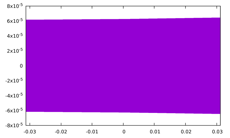
(a) Naive interval arithmetic.

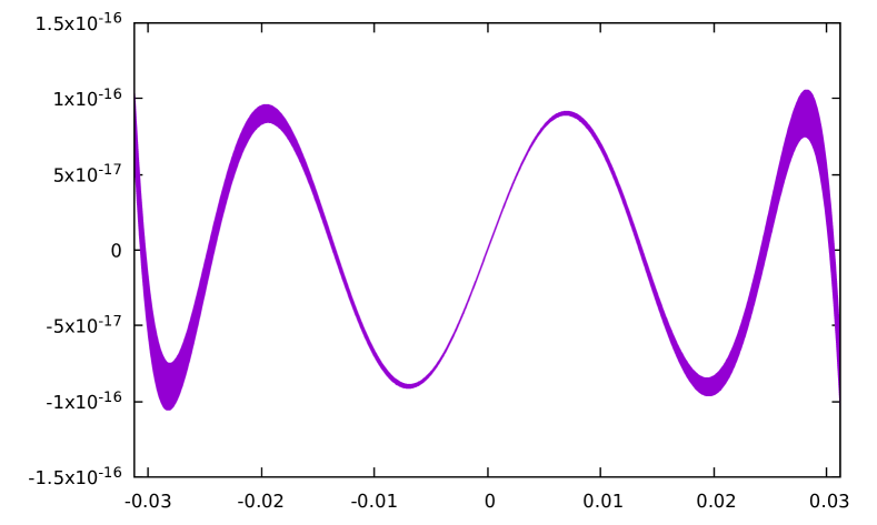
(b) Completeness check disabled.

Figure 2: Correct but hardly complete variants of Figure 1(c).

There is a second, more practical, reason for not using naive interval arithmetic. Since we are performing all our computations in the logic of Coq, evaluating $w=512$ instances of the interval implementation of cosine might take too long for an interactive use of Coq. The solution is to compute a rigorous polynomial approximation $(p,\Delta)$ of $f$ over some large interval $X$, ideally $W=[\mathit{ox};\mathit{ox}+\mathit{dx}\cdot w]$:

$$\forall x\in X,~{}p(x)-f(x)\in\Delta.$$

The idea of using these polynomial approximations originated from Sollya [2]. They were later formalized in Coq [4]. Eventually, they joined the CoqInterval library [5].

These polynomial approximations were instrumental when devising the integral tactic for guaranteed numerical quadrature [3]. Indeed, once $(p,\Delta)$ has been computed, one can easily enclose the integrals of $p(x)$ and of $p(x)-f(x)$ over $X$, and thus the integral of $f(x)=p(x)-(p(x)-f(x))$ over $X$. Since the ability to numerically integrate a function is not that different from the ability to accurately plot its graph, we follow a similar approach here. Once $(p,\Delta)$ has been computed, we use it to compute an enclosure $Y_{\_}i$ of $f(X_{\_}i)$. This time, we can use naive interval arithmetic to evaluate $Y_{\_}i=p(X_{\_}i)+\Delta$.

If $p$ has degree $0$, then the result is similar to the one obtained using naive interval arithmetic. With degrees $1$ and $2$, the plot is still an indiscriminate block of pixels, though the bounds are less overapproximated. With degree $3$, losses of correlation at the pixel level are completely accounted for. So, the plot looks fine, but computing it is way too slow for interactive use. Indeed, a single polynomial is not sufficient for the whole interval $W$, since there is no way a degree-3 polynomial could ever meaningfully approximate a function with 7 roots. So, the interval $W$ has to be split into many subintervals $X$, on each of which $p$ has to be computed. The best running time is obtained for degree 6. Then, the higher the degree, the slower it gets. Indeed, decreasing the number of subintervals no longer compensates the increasing cost of computing $p$ and evaluating it for every pixel. The optimal degree highly depends on the plot, so its choice is left to the user. By default, degree 10 is used, as with tactic integral.

Thanks to the rigorous polynomial approximations, we now have a correct plot that is formally verified. But as shown on Figure 2(a), a correct plot is not necessarily a complete one. So, to increase the usability of our approach, we would like the plot to never be more than a few pixels wide. A first idea would be to measure the width of $p(X_{\_}i)$. If it is larger than a few pixels, then $X$ needs to be subdivided further. Unfortunately, this causes too many subdivisions when the function varies quickly, which is the case at the left and right ends of Figure 1(c). A second idea would be to measure the width of the error interval $\Delta$ to decide whether $X$ is sufficiently small. Unfortunately, this still does not work. Indeed, the further from the center of $X$, the worst the loss of correlation becomes when evaluating $p(X_{\_}i)$, to the point where it becomes noticeable, as shown on Figure 2(b). So, this time, there are not enough subdivisions.

To strike a balance between these two issues, the code computes an underestimation of $f$ over $X_{\_}i$ and compares it to the overestimation $Y_{\_}i=p(X_{\_}i)+\Delta$. If the latter is only a few pixels larger than the former, then it is deemed good enough. Concretely, the code computes $Z=p(\mathrm{lower}(X_{\_}i))+\Delta$. There is a value of $x\in X_{\_}i$ such that $f(x)$ lies between the lower bound of $Y_{\_}i$ and the upper bound of $Z$. So, if the distance between these two bounds is smaller than a few pixels, the lower bound of $Y_{\_}i$ is accurate enough. If not, the code tries again with the upper bound of $Z^{\prime}=p(\mathrm{upper}(X_{\_}i))+\Delta$. If the lower bound of $Y_{\_}i$ is accurate enough, the code then checks the upper bound by comparing it to the lower bounds of $Z$ and $Z^{\prime}$.

To finish, there is some kind of a chicken-or-egg problem. If the user has not provided $\mathit{dy}$, how does the code know the height of a pixel used to check for pseudo-completeness? To estimate it, the code samples the function at 50 uniformly spaced points of $W$. This gives an underestimation of $[y_{\_}1;y_{\_}2]$ and thus of $\mathit{dy}$. If the sampled values do not capture the extreme values of the function, then the predicted value of $\mathit{dy}$ is too small, which causes the plot to be uselessly accurate and thus slower to compute.

4 Interface

We now have an algorithm (run inside the logic of Coq) that, given some reification of function $f$ and some values for $\mathit{ox}$, $\mathit{dx}$, etc, computes a list $\ell$ of pairs of integers. We also have a theorem formally verified in Coq that states (plot2 $f$ $\mathit{ox}$ … $\ell$). So, only interface issues remain.

First, let us deal with the plot display. The list $\ell$ is almost a run-length encoding of the function graph, assuming a column-major order. Indeed, a pair $(y_{\_}1,y_{\_}2)\subseteq[0;h]$ of integers represents a column of first $y_{\_}1$ blank pixels, then $y_{\_}2-y_{\_}1$ filled pixels, and finally $h-y_{\_}2$ blank pixels. Getting Gnuplot to draw the resulting bitmap is easy. Unfortunately, it is difficult to make sure that Gnuplot maps one pixel of the bitmap to exactly one pixel of the screen. As a consequence, some features of the plot might disappear if the drawing area is just one pixel too small. Conversely, if the user tells Gnuplot to zoom in (or just enlarges the drawing window), then the plot starts looking blocky.

So, rather than a bitmap, it is visually more satisfying to turn the plot into two piecewise affine curves that enclose the filled pixels of the bitmap. This vector encoding allows the user to freely zoom on the plot or resize the Gnuplot windows. Computing these two curves is actually quite easy. Given two consecutive elements of the list $\ell_{\_}{i-1}=(y_{\_}1,y_{\_}2)$ and $\ell_{\_}i=(y^{\prime}_{\_}1,y^{\prime}_{\_}2)$, one just needs to associate to abscissa $\mathit{ox}+i\cdot\mathit{dx}$ the ordinates $\mathit{oy}+\min(y_{\_}1,y^{\prime}_{\_}1)\cdot\mathit{dy}$ and $\mathit{oy}+\max(y_{\_}2,y^{\prime}_{\_}2)\cdot\mathit{dy}$. The band between the two curves contains all the filled pixels of the original bitmap, thus guaranteeing the correctness of the plot, at the expense of being a bit less narrow than the bitmap one.

As for the user queries, let us take some inspiration from existing computer algebras system. They often handle plots as first-class citizen, that is, the user can execute “p := plot(f,x1,x2)” to store a function graph into some variable p. Then, simply executing p causes the plot to be displayed. (Both steps can usually be merged into a single one, if the function graph does not need to be stored for later use.) We can follow a similar approach for Coq. Unfortunately, Coq requires top-level terms to be preceded by a command, e.g., Print, Check, About. We cannot reuse an existing command, so we add yet another one: Plot p. This causes Coq to open a Gnuplot windows using the data encoded in the plot2 type of p. As for a Coq equivalent to “p := plot(f,x1,x2)”, we combine the Definition command with the tactic-in-term feature of Coq. This provides the following interface: Definition p := ltac:(plot f x1 x2). The plot tactic can take two extra arguments to specify the ordinate range. When absent, the tactic computes the extrema of the function between the endpoints.

The plot tactic supports the same configuration mechanism as the tactics interval and integral [5]. For instance, to obtain Figure 1(c), one needs to increase the precision to 90 bits, as follows:

⬇

plot (fun x => 1+x*... - exp x) (-1/32) (1/32) with (i_prec 90)

A new flag has been added to specify the dimension of the bitmap: i_size w h. By default, the tactic produces a plot of size $512\times 384$. Other meaningful flags are i_degree to control the degree of the polynomial approximations and i_native_compute to tell Coq to first compile the algorithm to machine code rather than directly interpreting it. This might be useful to speed up some computationally-intensive plots. Indeed, the architecture of Coq unfortunately forces the tactic to execute the algorithm twice: once to get the actual list and a second time to instantiate the correctness theorem.

5 Conclusion

This article has presented a mechanism integrated in release 4.2 of the CoqInterval library. It makes it possible to compute formally correct function graphs and display them directly from Coq. Despite the computations being performed inside the logic of Coq, performances are good enough for interactive use. For example, it takes less than 4 seconds to compute and formally verify the complicated plot of Figure 1(d) with the default settings, and about 1 second with i_native_compute.

While the current interface is a bit unfriendly, we could readily imagine a new front-end that would exempt the user from typing Definition and Plot, as well as the ltac:(...) quotation mechanism. The long-term goal is to revisit the way Coq is used, making it more of a computer algebra system, e.g., through interfaces such as CoCalc and Jupyter [7]. Plots would no longer be opened in separate windows but directly embedded in the document. In the meantime, by virtue of the plotting algorithm being written in Gallina, it could easily be extracted to OCaml and distributed as a standalone library.

References

- [1]
- [2] Sylvain Chevillard, Mioara Joldeş & Christoph Lauter (2010): Sollya: An Environment for the Development of Numerical Codes. In Komei Fukuda, Joris van der Hoeven, Michael Joswig & Nobuki Takayama, editors: 3rd International Congress on Mathematical Software (ICMS), Lecture Notes in Computer Science 6327, Kobe, Japan, pp. 28–31, 10.1007/978-3-642-15582-65.
- [3] Assia Mahboubi, Guillaume Melquiond & Thomas Sibut-Pinote (2019): Formally Verified Approximations of Definite Integrals. Journal of Automated Reasoning 62(2), pp. 281–300, 10.1007/s10817-018-9463-7.
- [4] Érik Martin-Dorel, Micaela Mayero, Ioana Pasca, Laurence Rideau & Laurent Théry (2013): Certified, Efficient and Sharp Univariate Taylor Models in Coq. In: 15th International Symposium on Symbolic and Numeric Algorithms for Scientific Computing (SYNASC), Timisoara, Romania, pp. 193–200, 10.1109/SYNASC.2013.33.
- [5] Érik Martin-Dorel & Guillaume Melquiond (2016): Proving Tight Bounds on Univariate Expressions with Elementary Functions in Coq. Journal of Automated Reasoning 57(3), pp. 187–217, 10.1007/s10817-015-9350-4.
- [6] Russell O’Connor (2008): A Computer Verified Theory of Compact Sets. In: Symbolic Computation in Software Science Austrian-Japanese Workshop (SCSS), RISC-Linz Report Series, pp. 148–162.
- [7] Fernando Pérez & Brian E. Granger (2007): IPython: a System for Interactive Scientific Computing. Computing in Science and Engineering 9(3), pp. 21–29, 10.1109/MCSE.2007.53.