Critical collapse of an axisymmetric ultrarelativistic fluid in $2+1$ dimensions

Abstract

We carry out numerical simulations of the gravitational collapse of a rotating perfect fluid with the ultrarelativistic equation of state $P=\kappa\rho$, in axisymmetry in $2+1$ spacetime dimensions with $\Lambda<0$. We show that for $\kappa\lesssim 0.42$, the critical phenomena are type I, and the critical solution is stationary. The picture for $\kappa\gtrsim 0.43$ is more delicate: for small angular momenta, we find type II phenomena, and the critical solution is quasistationary, contracting adiabatically. The spin-to-mass ratio of the critical solution increases as it contracts, and hence, so does that of the black hole created at the end as we fine-tune to the black-hole threshold. Forming extremal black holes is avoided because the contraction of the critical solution smoothly ends as extremality is approached.

I Introduction

Critical collapse is concerned with the threshold of black-hole formation in the space of initial data. Starting with Choptuik’s study of the spherically symmetric, massless scalar field [1], and since then generalized to many other systems [2], one can enumerate several general features of critical phenomena. The more interesting kind is now called “type II” phenomena. As the black-hole threshold is approached through the fine-tuning of a one-parameter family of initial data, the black-hole mass and spacetime curvature scale as a power of distance to the black-hole threshold. Furthermore, for initial data close to the black-hole threshold, the solution will be, in an intermediary stage, well approximated by a critical solution. This critical solution has the general characteristics of being self-similar, universal (independent of the initial data) and possessing a single growing linear perturbation mode. By contrast, in “type I” phenomena, the mass and curvature do not scale, but instead approach a nontrivial constant. The critical solution is time periodic or stationary. The above properties for type I and II phenomena hold for all matter systems studied thus far in $3+1$ and all higher dimensions; see Ref. [2] for a review.

The vast majority of research studies dedicated to critical collapse focuses on spherically symmetric initial data. Since black holes can carry angular momentum, the full picture of critical collapse requires us to go beyond spherical symmetry. However, the generalization from spherically symmetric to, say, axisymmetric initial data brings about many numerical and theoretical complications. In part, one has to deal with an additional independent variable. Moreover, gravitational waves exist beyond spherical symmetry, and they can exhibit (type II) critical phenomena by themselves [3]. In particular, this implies that, if one wishes to study the critical phenomena of some matter field in axisymmetry, one will have to disentangle the critical phenomena due to the matter field and those due to gravitational waves. This additional difficulty is currently of great importance since the critical phenomena of pure gravitational waves are still poorly understood.

One way to work around those problems is to consider, as a toy model, the situation in $2+1$ dimensions. Gravity in $2+1$ dimensions is rather peculiar. Notably, black holes cannot form without a negative cosmological constant. The rotating black-hole solution, called the BTZ solution [4], is also quite unique. Its central singularity is not a usual curvature singularity, but a causal singularity. Furthermore, the black-hole spectrum is separated from the background (anti-de Sitter spacetime) configuration by a mass gap. A direct consequence of this is that small deviations from anti-de Sitter spacetime (from now, AdS) cannot collapse into a black hole. Furthermore, gravitational waves do not exist in $2+1$ dimensions. For these reasons, it is unclear if many of the results in $2+1$ dimensions can simply be carried over to the $3+1$ dimensional setting. On the other hand, the absence of gravitational waves enables us to bypass the current major difficulties encountered in higher dimensions. A rotating object in $3+1$ dimensions cannot be spherically symmetric, but at most axisymmetric, roughly speaking because rotation tries to flatten the rotating body. In the $2+1$-dimensional counterpart of such rotating axisymmetric solutions, there is no dimension for the flattening to happen, in and all the variables are still only functions of “time” and “radius”. This makes the study of critical collapse with rotating initial data much more tractable. As in Refs [5, 6], we call a solution circularly symmetric if it admits a spacelike Killing vector $\partial_{\theta}$ with closed orbits. More specifically (and perhaps in a slight abuse of notation), we call it spherically symmetric if there is no rotation, and we call it axisymmetric with rotation.

Pretorius and Choptuik investigated the black-hole threshold for the spherically symmetric, massless scalar field in $2+1$ dimensions [7]. They found type II phenomena (mass and curvature scaling). The critical solution is also found, near the center, to be approximately continuously self-similar (as opposed to discretely as is the case in $3+1$ dimensions). This system was investigated in more depth in Ref. [8]. The authors found good agreement between the numerical solution during the critical regime and an exact continuously self-similar $\Lambda=0$ solution. However, one major unresolved issue is that this exact solution has three growing modes. Investigating the modes numerically, they surprisingly only find numerical evidence of the top (largest) growing mode. There is to date no satisfactory explanation for this, but it was conjectured that the nonlinear effect of the cosmological constant may be responsible for removing all but the top growing mode (adding the effect of the cosmological constant perturbatively does not alter the perturbation spectrum).

In Ref. [5], the same authors generalized the consideration to a complex rotating scalar field. It turns out that the effect of rotation is highly nontrivial; neither the critical exponents nor the critical solution are universal. The angular momentum does not show any scaling. The mass and curvature may or may not scale, depending on the one-parameter family of initial data. Finally, the threshold of mass and curvature scalings are different.

In Ref. [6], the present authors investigated the spherically symmetric perfect fluid, with barotropic equation of state $P=\kappa\rho$. We found that the critical phenomena are of type I if $\kappa\lesssim 0.42$, while they are of type II if $\kappa\gtrsim 0.43$. The critical solution for type I is static (as expected), but for type II, it is not self-similar, but instead quasistatic. That is, the critical solution corresponds to an adiabatic sequence of static solutions whose size shrinks to zero (exponentially).

In this paper, we now extend this previous work to axisymmetric initial data. In Sec. II, we give a quick overview of the Einstein-fluid matter system. In Sec. III, we present and discuss our numerical findings.

II Einstein and Fluid equations in polar-radial coordinates

We refer the reader to the companion paper [9] for a complete discussion. We use units where $c=G=1$.

In axisymmetry in $2+1$ dimensions, we introduce generalized polar-radial coordinates as

$$ds^{2} = -\alpha^{2}(t,r)\,dt^{2}+a^{2}(t,r)R^{\prime 2}(r)\,dr^{2}$$ (1)

$$+R^{2}(r)[d\theta+\beta(t,r)dt]^{2}.$$

We denote $\partial/\partial t$ by a dot and $\partial/\partial r$ by a prime. Note that our choice $g_{rr}=a^{2}R^{\prime 2}$ makes $a$ invariant under a redefinition of the radial coordinate, $r\to\tilde{r}(r)$. The “area” (circumference) radius $R$ is defined geometrically as the length of the Killing vector $\partial/\partial\theta$.

We impose the gauge condition $\alpha(t,0)=1$ ($t$ is proper time at the center), and the regularity condition $a(t,0)=1$ (no conical singularity at the center).

We define the auxiliary quantity

$$\gamma:=\beta^{\prime},$$ (2)

anticipating that $\beta$ will not appear undifferentiated in the Einstein or fluid equations, but only in the form of $\gamma$ and its derivatives, since the form (1) of the metric is invariant under the change of angular variable $\theta\to\theta+f(t)$. It follows that the particular choice of gauge for $\beta$ does not affect our evolution, and for our numerical implementation, we choose $\beta(t,0)=0$. The gauge is fully specified only after specifying the function $R(r)$. In our numerical simulations, we use the compactified coordinate

$$R(r)=\ell\tan(r/\ell),$$ (3)

where

$$\ell:={1\over\sqrt{-\Lambda}}$$ (4)

is the AdS length scale, but for clarity we write $R$ and $R^{\prime}$ rather than the explicit expressions.

In our coordinates, the Kodama mass $M$ and angular momentum $J$ are given by

$$J(t,r) := {R^{3}\gamma\over R^{\prime}a\alpha},$$ (5)

$$M(t,r) := {R^{2}\over\ell^{2}}-{1\over a^{2}}+{J^{2}\over 4R^{2}}.$$ (6)

This local mass function generalizes the well-known Misner-Sharp mass from spherical symmetry (in any spacetime dimension) to axisymmetry (in $2+1$ only) [9, 10].

The stress-energy tensor for a perfect fluid is

$$T_{ab}=(\rho+P)u_{a}u_{b}+Pg_{ab},$$ (7)

where $u^{a}$ is tangential to the fluid worldlines, with $u^{a}u_{a}=-1$, and $P$ and $\rho$ are the pressure and total energy density measured in the fluid frame. In the following, we assume the one-parameter family of ultrarelativistic fluid equations of state $P=\kappa\rho$, where $0<\kappa<1$.

The 3-velocity is decomposed as

$$u^{\mu}=\{u^{t},u^{r},u^{\theta}\}=\Gamma\left\{\frac{1}{\alpha},\frac{v}{aR^{\prime}},{w\over R}-\frac{\beta}{\alpha}\right\},$$ (8)

where $v$ and $w$ are the physical radial and tangential velocities of the fluid relative to observers at constant $R$, satisfying $v^{2}+w^{2}<1$, and

$$\Gamma:=\left(1-v^{2}-w^{2}\right)^{-1/2}$$ (9)

is the corresponding Lorentz factor.

The stress-energy conservation law $\nabla_{a}T^{ab}=0$, which together with the equation of state governs the fluid evolution, can be written in balance law form

$${\bf q}_{,t}+{\bf f}_{,r}={\bf S},$$ (10)

where we have defined the conserved quantities

$${\bf q}:=\{\Omega,Y,Z\}$$ (11)

given by

$$Y := R^{\prime}v\sigma,$$ (12)

$$Z := aR^{2}R^{\prime}w\sigma,$$ (13)

$$\Omega := R^{\prime}R\tau+{JZ\over 2R^{2}},$$ (14)

the corresponding fluxes ${\bf f}$ given by

$$f_{(Y)} := {\alpha\over a}(P+v^{2}\sigma),$$ (15)

$$f_{(Z)} := \alpha R^{2}vw\sigma,$$ (16)

$$f_{(\Omega)} := {\alpha\over a}Rv\sigma+{Jf_{(Z)}\over 2R^{2}},$$ (17)

the corresponding sources ${\bf S}$ given by

$$S_{(Y)} = {1\over a}\Bigl{[}(w^{2}-v^{2})\sigma\alpha{R^{\prime}\over R}-\tau\alpha_{,r}$$ (18)

$$-(P+v^{2}\sigma)\alpha(\ln a)_{,r}$$

$$+Rw\sigma\gamma-2v\sigma R^{\prime}a_{,t}\Bigr{]},$$

$$S_{(Z)} = 0,$$ (19)

$$S_{(\Omega)} = 0,$$ (20)

and the shorthands

$$\sigma := \Gamma^{2}(1+\kappa)\rho,$$ (21)

$$P := \kappa\rho,$$ (22)

$$\tau := \sigma-P.$$ (23)

At any given time, the balance laws (10) are used to compute time derivatives of the conserved quantities ${\bf q}$, using standard high-resolution shock-capturing methods. The ${\bf q}$ are evolved to the next time step via a fourth-order Runge-Kutta step. At each (sub-)time step, the metric variables are then updated through the Einstein equations

$$M_{,r} = 16\pi\Omega,$$ (24)

$$J_{,r} = 16\pi Z,$$ (25)

$$(\ln\alpha a)_{,r} = 8\pi a^{2}RR^{\prime}(1+v^{2})\sigma.$$ (26)

Our numerical scheme is totally constrained, in the sense that only the matter is updated through evolution equations. Our numerical scheme exploits the conservation laws for $\Omega$ and $Z$, and in consequence for $M$ and $J$, to make their numerical counterparts exactly conserved in the discretized equations.

III Numerical results

III.1 Initial data

The numerical grid is equally spaced in the compactified coordinate $r$, as defined in (3), with $800$ grid points. We fix the cosmological constant to be $\Lambda=-\pi^{2}/4$, so that the AdS boundary is located at $r=1$. The numerical domain does not comprise the entire spacetime. Instead, we set an unphysical outer boundary with “copy boundary conditions” for the conserved variables ${\bf q}$. Unless otherwise stated, we fix the numerical outer boundary at $r=0.7$, corresponding in area radius to $R_{\text{max}}\simeq 1.25\simeq 1.96\ell$.

We choose to initialize the primitive fluid variables $\rho$ and $v$ as double Gaussians in $R$,

$$\rho(0,R) = \frac{p_{\rho}}{2}\left(e^{-\left(\frac{R-R_{\rho}}{\sigma_{\rho}}\right)^{2}}+e^{-\left(\frac{R+R_{\rho}}{\sigma_{\rho}}\right)^{2}}\right),$$

$$v(0,R) = \frac{p_{v}}{2}\left(e^{-\left(\frac{R-R_{v}}{\sigma_{v}}\right)^{2}}+e^{-\left(\frac{R+R_{v}}{\sigma_{v}}\right)^{2}}\right),$$ (28)

where $p_{\rho}$ and $p_{v}$ are the magnitudes, $R_{\rho}$ and $R_{v}$ the displacements from the center, and $\sigma_{\rho}$ and $\sigma_{v}$ the widths of the Gaussians. The initial data for $w$ are defined through the combination $w\Gamma^{2}$, by

$$w(0,R)\Gamma^{2}=p_{w}R.$$ (29)

Near the center, the fluid is “rigidly rotating” in the sense that $w\sim R$. The strength of the rotation is parametrized by $p_{w}$.

As for the spherically symmetric case, we consider three types of initial data:

1) time-symmetric off-centered: $p_{v}=0$, $R_{\rho}=0.4$,

2) time-symmetric centered: $p_{v}=0$, $R_{\rho}=0$, and

3) initially ingoing off-centered: $p_{v}=-0.15$, $R_{v}=0.4$, $\sigma_{v}=0.15$, $R_{\rho}=0.4$.

In all cases, for $\kappa\leq 0.42$, we take $\sigma_{\rho}=0.05$, while for $\kappa\geq 0.43$, we choose $\sigma_{\rho}=0.2$. The reason for this choice is the fact that in spherical symmetry, where type I behavior occurs, numerical instabilities form near the numerical outer boundary and travel inwards. These instabilities form strong shocks near the center for a second-order limiter. Making the initial data more compact partially mitigates this. Furthermore, for $\kappa\leq 0.42$, we use a first-order (Godunov) limiter, as we did in spherical symmetry. The dissipative properties of the Godunov limiter eliminate those shocks. As we see, similar instabilities now also occur for $\kappa\gtrsim 0.43$, for “large” deviations from spherical symmetry. Unless otherwise stated, we therefore also use a Godunov limiter for $\kappa\geq 0.43$, although we keep the width as $\sigma_{\rho}=0.2$.

Finally, in all cases, $p_{w}$ is fixed to a particular value, and $p_{\rho}=:p$ is the parameter to be fine-tuned to the black-hole threshold.

We use the same conventions as in [6] and denote by $p=p_{\star}$ the critical parameter separating initial data that (promptly) collapse and disperse. We are interested in initial data where $p\simeq p_{\star}$, and we denote by sub$n$ subcritical data for which $\log_{10}(p_{\star}-p)\simeq-n$, and by super$n$ supercritical data with $\log_{10}(p-p_{\star})\simeq-n$.

In the following, “apparent horizon” (AH) mass and angular momentum refer to the first appearance of a marginally outer-trapped surface in our time slicing, indicated by diverging metric component $a$.

III.2 $\kappa\lesssim 0.42$: Type I critical collapse

III.2.1 Lifetime scaling

In the spherically symmetric case, we showed in Ref. [6] that the critical phenomena depend on the value of $\kappa$. In particular, for $\kappa\lesssim 0.42$, we find typical type I behavior, where the mass and curvature do not scale and the critical solution near the center is static. How is this picture modified in the presence of angular momentum?

We start answering this question by showing, in Fig. 1, a log-log plot of the apparent horizon mass $M_{\text{AH}}$ (green group of curves), the adimensionalized apparent horizon angular momentum $J_{\text{AH}}/\ell$ (blue group of curves), and the maximum of curvature $-\Lambda\rho_{\text{max}}^{-1}$ (orange group of curves), against $p-p_{\star}$, for different values of $p_{\omega}$. For all these plots, we consider centered initial data with $\kappa=0.4$. The range of $p_{\omega}$ is $p_{\omega}=0.01$, $0.1$, $0.2$, $0.4$, $0.6$, $0.8$ and $1.0$. This corresponds to a range from “small” angular momentum (in the sense that $J_{\text{AH}}/(M_{\text{AH}}\ell)\ll 1$) to “large” angular momentum (for example, $p_{\omega}=1.0$ corresponds to $J_{\text{AH}}/(M_{\text{AH}}\ell)\simeq 0.64$).

This behavior, as in spherical symmetry, persists up to some critical value of $\kappa$ between $\kappa=0.42$ and $\kappa=0.43$. For comparison, we have also added an evolution with $\kappa=0.43$ (dotted curves) and $p_{\omega}=0.01$. The type I behavior also holds for the off-centered and ingoing initial data.

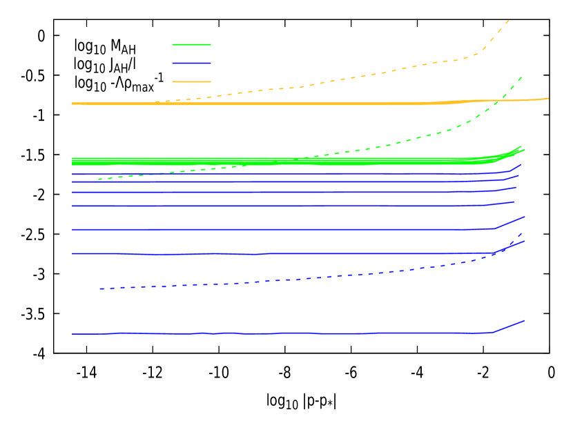
Figure 1: Log-log plot demonstrating the absence of scaling, for small $\kappa$, of $\rho_{\text{max}}$ (upper group of curves, orange), $M_{\text{AH}}$ (middle group of curves, green ) and $J_{\text{AH}}/\ell$ (bottom group of curves, blue ) for different values of $p_{\omega}$, corresponding to a range of “small” to “large” angular momenta. Solid lines correspond to $\kappa=0.4$. We find typical type I behavior, irrespective of $p_{\omega}$. This behavior still holds up to $\kappa=0.42$. For comparison, the dotted curves show $\kappa=0.43$ and “small” angular momentum, where type II behavior is instead observed within this range of fine-tuning, see Fig. 4 for more details.

As in the spherically symmetric case, we consider the time-dependent quantity $R_{M}$, defined by

$$M(t,R_{M}(t)):=0,$$ (30)

as a measure of the length scale of the solution. Similarly, we define the central density $\rho_{0}$, mass $M_{\text{OB}}$, and angular momentum $J_{\text{OB}}$ at the numerical outer boundary,

$$\rho_{0}(t) := \rho(t,0),$$ (31)

$$M_{\text{OB}}(t) := M(t,R_{\text{max}}),$$ (32)

$$J_{\text{OB}}(t) := J(t,R_{\text{max}}).$$ (33)

In Fig. 2, we plot in a linear-log plot, $\sqrt{-\Lambda\rho_{0}^{-1}}$, $J_{\text{OB}}/\ell$, $\sqrt{M_{\text{OB}}}$, and $R_{M}/\ell$ against central proper time $t$, for sub6 to sub15 initial data. We consider here centered initial data with $p_{\omega}=1.0$. Note that we have shifted $\log_{10}J_{\text{OB}}/\ell$ by a constant $c=1.2$ for clarity. As is typical for critical phenomena, the more fine-tuned the initial data to the black-hole threshold, the longer the critical regime, before the growing mode of the critical solution becomes dominant. In order to avoid cluttering, we truncate the plots after it is clear that the growing mode causes the curves to “peel off” from the critical regime.

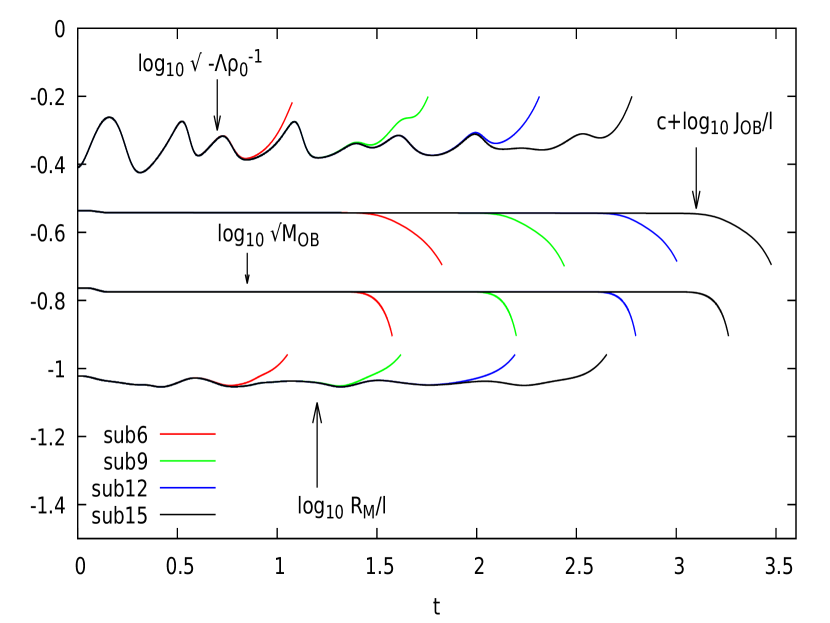
Figure 2: Lin-log plot of $R_{M}(t)/\ell$, $\sqrt{-\Lambda\rho_{0}^{-1}(t)}$, $\sqrt{M_{\text{OB}}(t)}$, and $J_{\text{OB}}(t)/\ell+c$ with $c=1.2$, for sub6 to sub15 centered initial data with $p_{w}=1.0$. We observe that, as we fine-tune to the black-hole threshold, the solution approaches an intermediate attractor solution in which all the variables are approximately constant. Less fine-tuned initial data peel off from the critical regime sooner than more fine-tuned data.

For type I phenomena, it is not the mass and curvature that scale. Instead, it is the lifetime of the intermediate regime where the solution is approximated by the critical solution. Assuming that the critical solution is stationary, we can make the following ansatz for its linear perturbations:

$$\delta Z(t,R)=\sum_{i=0}^{\infty}C_{i}(p)\,e^{\sigma_{i}{t\over\ell}}\,Z_{i}(R),$$ (34)

where $Z$ stands for any dimensionless metric or matter variable, such as $R^{2}\rho$, $M$, or $\alpha$.

We assume the critical solution has a single growing mode, ${\rm Re}\,\sigma_{0}>0$. Since the solution is exactly critical at $p=p_{\star}$, this implies that $C_{0}(p)\sim p-p_{\star}$. We define the time $t=t_{p}$ to be the time where the growing perturbation becomes nonlinear. This occurs when

$$(p-p_{\star})e^{\sigma_{0}{t_{p}\over\ell}}\simeq 1,$$ (35)

and so

$$t_{p}=\frac{\ell}{\sigma_{0}}\ln|p-p_{\star}|+\text{constant}.$$ (36)

The exponent $\sigma_{0}$ can be read off from Fig. 2. We find $\sigma_{0}\simeq 8.29$, close to its value in spherical symmetry (which was $\simeq 8.84$) [6].

III.2.2 The critical solution

In [11], we showed the existence of a two-parameter family of rigidly rotating, stationary star solutions for any causal equation of state $P=P(\rho)$. These solutions are analytic everywhere including at the center, and have finite total mass $M$ and angular momentum $J$. The two free parameters can be taken to be $s$, giving the overall length scale of the star, and $\tilde{\Omega}$, parametrizing the rotation of the star. The latter is defined so that $\tilde{\Omega}=0$ corresponds to nonrotating stars. We can write these exact solutions as

$$Z(R)=\check{Z}\left({R\over s};\mu,\tilde{\Omega}\right),$$ (37)

where $\check{Z}$ is the corresponding exact stationary solutions. The cosmological constant enters this picture through a specific combination, parametrized by the dimensionless quantity $\mu$,

$$\mu:=-\Lambda s^{2}-\tilde{\Omega}^{2}.$$ (38)

In what follows, all quantities pertaining to the exact stationary solutions have a check symbol, as in (37).

The parameters $\mu$ and $\tilde{\Omega}$ correspond to $\mu$ and $\Omega$ in [11]. (The tilde is used to distinguish $\tilde{\Omega}$ from the unrelated conserved variable $\Omega$). Regular stationary solutions exist only for $0\leq\mu\leq 1$, and $\mu$ can be interpreted as parametrizing the competition of the attractive acceleration induced by a negative cosmological constant and the centrifugal acceleration.

In Fig. 3, we compare our best subcritical numerical solution at $t=2.1$, where the solution is approximately stationary, to the family of stationary solutions. Since the stationary solutions form a two-parameter family, we need to fit those two parameters. For this, we match the central density and total angular momentum, using the angular momentum at the numerical outer boundary as a proxy for the total angular momentum. The matching conditions are

$$J_{\text{OB}}(1-\kappa) \equiv 4\kappa\ell(1-\mu)\tilde{\Omega}\sqrt{\mu+\tilde{\Omega}^{2}},$$ (39)

$$1-\mu \equiv 8\pi\kappa\rho_{0}\ell^{2}(\mu+\tilde{\Omega}^{2}).$$ (40)

Note that there is a slight abuse of language here; the total angular momentum (and mass) of the system is a conserved quantity. The angular momentum (and mass) at the numerical outer boundary (at finite radius) differ from it, since a bit of spin (and mass) are radiated away through this boundary at the start of the evolution, when the solution has yet to enter the critical regime. At late times, the approximately time-independent value of the angular momentum (and mass) at the outer boundary during the critical regime is a fixed fraction of the constant total spin (and mass) of the system.

Our matching of the angular momentum therefore introduces a small systematic error. At first, we attempted to ask for the value of $R_{M}$ between the numerical and exact solutions to agree. This is also possible, but $R_{M}$ depends very weakly on rotation. Such a matching condition is therefore very sensitive to numerical error.

In the example of Fig. 3, our matching procedure gives $s\simeq 0.0882$ and $\tilde{\Omega}\simeq 0.0498$. We then find very good agreement for $\rho$, $M$ and $a/\alpha$ at all $R$. We find slightly less good agreement for the angular momentum. Since $J$ is relatively small, it is likely that this is a numerical error, although its precise nature is unknown.

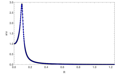
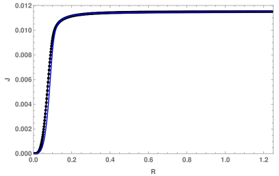
Figure 3: Comparison of the numerical solution for our best subcritical data during the critical regime (black dotted lines) with the exact stationary solutions (solid blue lines). For the numerical data, we chose here $\kappa=0.4$ with $p_{\omega}=1.0$.

We remark here that, at first, we attempted to push the numerical outer boundary further out. We noticed however, for $R_{\text{max}}\gtrsim 4$, there is a clear numerical error that builds up and causes mass and spin to slowly radiate away. For example, for $R_{\text{max}}\simeq 1.25$, the total mass and angular momentum stay constant in the critical regime within $\ll 1\%$ (see Fig. 7). On the other hand, for $R_{\text{max}}\simeq 4$, they decrease slowly and approximately linearly. As compared to the near constant value that they take for $R_{\text{max}}\simeq 1.25$, they further decrease by about $29\%$ and $16\%$ for $R_{\text{max}}\simeq 4$, respectively. This is measured up until the time when the “star” disperses. This decay rate is also different for larger $R_{\text{max}}$. We do not have an explanation for this numerical error.

III.3 $\kappa\gtrsim 0.43$: Type II critical collapse

III.3.1 Curvature and mass scaling

In spherical symmetry, we have given strong evidence that the critical phenomena are type II for $\kappa\geq 0.43$ (the apparent-horizon mass and curvature scale as some power law and the critical solution shrinks quasistatically to arbitrarily small size); see [6]. As we did for $\kappa\leq 0.42$, we now consider families of initial data with different initial angular momentum $p_{\omega}$. In the following, we focus our attention on the case $\kappa=0.5$.

In Fig. 4, we plot $-\Lambda\rho_{\text{max}}^{-1}$ (orange group of curves), $M_{AH}$ (green group of curves) and $J_{AH}/\ell$ (blue group of curves) as a function of $p-p_{\star}$ for centered initial data and with different $p_{w}$, namely, $p_{w}=0.02$, $0.04$, $0.06$, $0.08$, $0.1$, $0.16$, $0.2$, $0.3$, $0.4$ and $0.5$ (solid lines). The dashed-dotted lines were obtained with $p_{w}=0.2$, but using the monotonized central (MC) limiter.

This plot illustrates multiple points. First, for “small” initial spin, we find typical type II phenomena where the density, mass and spin scale like power laws. Second, the angular momentum $J_{\text{AH}}$ scales more slowly than $M_{\text{AH}}$. In particular, the spin-to-mass ratio of the resulting black hole increases as we fine-tune to the black-hole threshold; see also Fig. 6. For larger initial spin such as $p_{w}\geq 0.2$ (or respectively more fine-tuning for smaller $p_{\omega}$), the spin-to-mass ratio approaches extremality. It does not go beyond, however, because the critical solution becomes stationary and, as a result, the power-law scaling with respect to $p-p_{*}$ also smoothly levels off.

The phenomena highlighted above have also been checked to hold for the off-centered and initially ingoing data, although we chose not to include them in the plot to avoid cluttering.

Note that for the evolution using the MC limiter (dashed-dotted), the scaling stops abruptly and the spin-to-mass ratio seems to remain constant with further fine-tuning. For reasons that will be made clearer later, this is expected to be a numerical artifact: for relatively large spin-to-mass ratio, numerical instabilities are generated at the numerical outer boundary, similar to those we faced when simulating type I phenomena in the spherically symmetric case. These instabilities travel inward and produce shocks near the center, which are absent using a more dissipative limiter such as the first-order Godunov limiter.

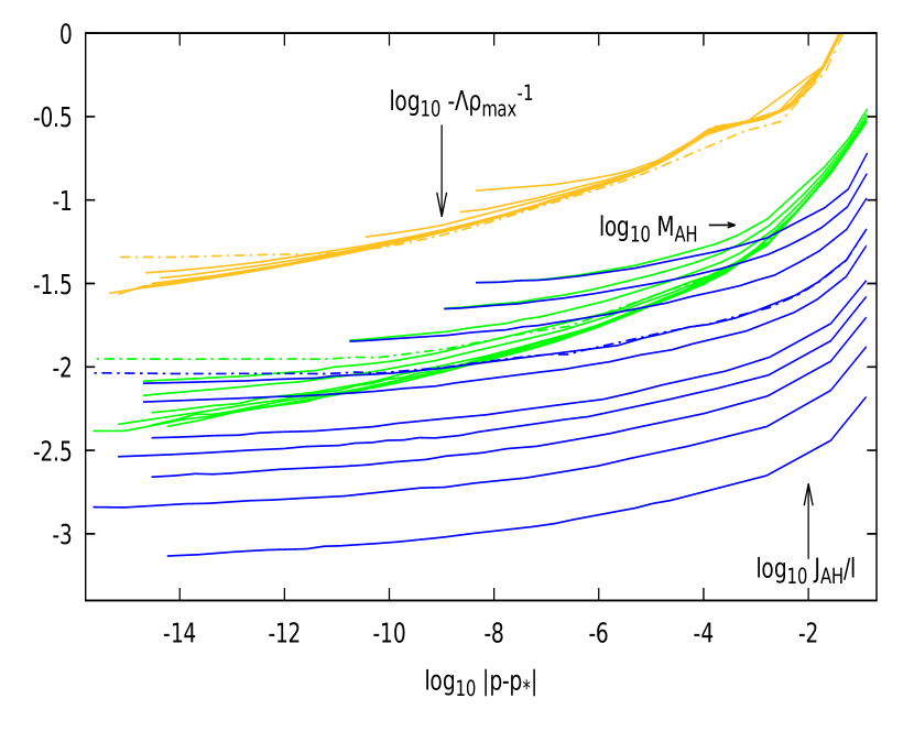
Figure 4: Log-log plot demonstrating the power-law scaling of $-\Lambda\rho_{\text{max}}^{-1}$ (orange, upper group of curves), $M_{\text{AH}}$ (green, middle group of curves) and $J_{\text{AH}}/\ell$ (blue, lower group of curves) for different values of $p_{w}$. Solid lines correspond to centered initial data, using the Godunov limiter. $J_{\text{AH}}$ decays more slowly than $M_{\text{AH}}$. For small spin-to-mass ratio, we find typical type II behavior, while for larger spin-to-mass ratio, the scaling smoothly flattens as extremality is approached. Dashed-dotted lines show an evolution with large initial spin ($p_{\omega}=0.2$), but using the MC limiter. There, the spin-to-mass ratio completely flattens beyond a certain level of fine-tuning, but this is a numerical artifact.

In Fig. 5, we explore the relationship between $J_{\text{AH}}$ and $M_{\text{AH}}$ more explicitly, for the critical solution and the final black hole. On the left, we show a parametric plot of $M_{\text{AH}}$ against $J_{\text{AH}}/\ell$ for the same initial data as in Fig. 4 (and using the same convention for the lines). We have added the bisections from the off-centered and ingoing initial data with $p_{w}=0.02$, $0.04$ and $0.06$ (dotted and dashed lines, respectively). The red line corresponds to $J_{\text{AH}}=M_{\text{AH}}\ell$. The trajectories in the $(M_{\text{AH}},J_{\text{AH}})$ plane are clearly family dependent, although as we increase the fine-tuning and the black holes become smaller (the bottom left corner) all the curves become approximately parallel to each other. This provides some evidence that the critical phenomena are controlled by a unique one-parameter family of critical solutions (universality).

On the right, we show a parametric plot of the mass $M_{\text{OB}}$ against the angular momentum $J_{\text{OB}}/\ell$, for our best supercritical data. As expected, both plots are qualitatively very similar, since one expects the mass and spin at the apparent horizon to be in some fixed ratio to their values at the numerical outer boundary, at the time when the solution veers off from the critical solution. It turns out that, for close to critical data, $M_{\text{AH}}\simeq M_{\text{OB}}$ and $J_{\text{AH}}\simeq J_{\text{OB}}$ at this time, and so this fixed fraction is almost one.

In Fig. 6, we use again the same data as in Fig. 5. On the left plot, we show the spin-to-mass ratio $J_{\text{AH}}/(M_{\text{AH}}\ell)$ as a function of $p-p_{\star}$ for different levels of fine-tuning. The only addition is a second bisection using a MC limiter (a second dashed-dotted curve), but where the numerical outer boundary is at $R_{\text{max}}\simeq 2.65\simeq 4.17\ell$. The fact that both dashed-dotted lines do not level off at the same spin-to-mass ratio gives evidence that the unphysical numerical outer boundary spoils the numerical results in that highly rotating regime. Instead, the results from the Godunov limiter, which removes the aforementioned instabilities, are more plausible; in the limit of fine-tuning, the black hole is extremal.

Similarly, in the right plot, we show the spin-to-mass ratio evaluated at the numerical outer boundary, for our best supercritical data, against proper time $t$. Both left and right plots are qualitatively similar. This is expected since the more fine-tuned the initial data are to the black-hole threshold, the longer it takes for the growing mode to dominate the perturbation, and so the more the spin-to-mass ratio can grow, before the solution collapses.

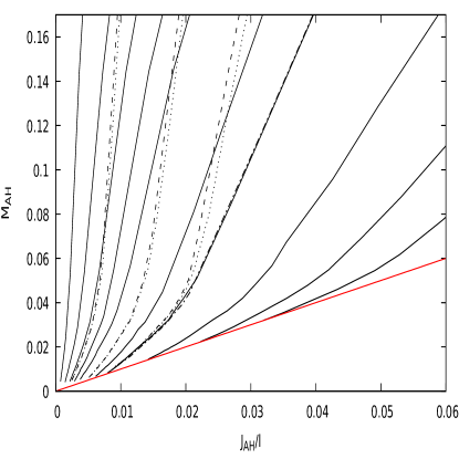
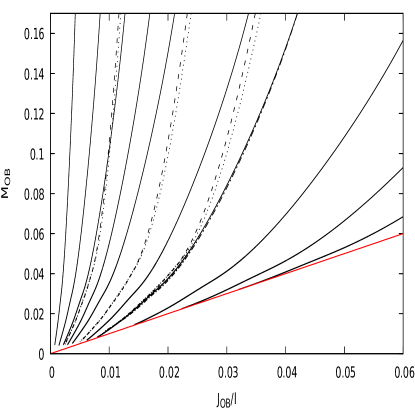
Figure 5: Left plot: parametric plot of the trajectories of $M_{\text{AH}}$ and $J_{\text{AH}}$ in Fig. 4 (solid and dashed-dotted lines), in the $M_{\text{AH}}$-$J_{\text{AH}}$ plane. The parameter along each curve is $p-p_{*}$. We have also added the trajectories of off-centered (dotted lines) and ingoing (dashed lines) initial data for three different values of $p_{w}$. The red line corresponds to $J_{\text{AH}}=M_{\text{AH}}\ell$. Right plot: a similar plot, using the same convention, except that we now consider the mass and angular momentum evaluated at the numerical outer boundary, for our best supercritical data. The parameter along each curve is now time.

If we define the time where the critical regime starts to be the time from which the central density shows critical scaling (at least for small rotation), then this occurs at $t\simeq 0.8$ for centered initial data (see, for example, Fig. 7), while it occurs at $t\simeq 1.0$ for ingoing and off-centered initial data. In the right plot of Fig. 6, the different trajectories do not cross during this critical regime. This again provides evidence that, in a suitable adiabatic limit, a given pair $(M_{\text{AH}},J_{\text{AH}})$ in a quasistationary sequence uniquely determines its evolution.

Figure 6: Left plot: log-log plot of $J_{\text{AH}}\over M_{\text{AH}}\ell$ against $p-p_{\star}$, for the same data as in Fig. 5, with the addition of a second dashed-dotted curve using the MC limiter but with a larger grid. The spin-to-mass ratio approaches extremality as we fine-tune to the black-hole threshold, except for the two MC limiter cases. Right plot: parametric plot of $J_{\text{OB}}\over M_{\text{OB}}\ell$, as a function of time $t$, for our best supercritical evolutions. The critical regime begins at $t\simeq 0.8$ for centered initial data, and at $t\simeq 1.0$ for ingoing and off-centered initial data.

III.3.2 The critical solution

We have seen in Fig. 5 that for sufficient fine-tuning (on the left) or at sufficiently late times (on the right), the trajectories in the $J$-$M$ plane do not cross, providing evidence that there is a universal one-parameter family of critical solutions that fibrates the $J$-$M$ plane. Independently, the fact that we can make arbitrarily small black holes or arbitrarily large central densities by fine-tuning generic one-parameter families of initial data suggests that each member of this family of critical solutions has precisely one unstable perturbation mode.

As in the spherically symmetric case, the profile of the solution can be roughly split into two regions: one central region where most of the density lies and whose size shrinks in time and an outer region (“atmosphere”) where the mass and spin are approximately constant in space and decrease to zero (exponentially) in time.

At a stage where the effect of spin can still be regarded as perturbative, one would expect the critical solution to be approximated by the quasistatic solution in spherical symmetry, plus a (unique, growing) nonspherical perturbation proportional to $p_{w}$ that carries the angular momentum. In particular, one would expect that the solution shrinks exponentially quickly in time.

To confirm this, we plot, on the left of Fig. 7, the logarithms of $R_{M}(t)/\ell$, $\sqrt{-\Lambda\rho_{0}^{-1}(t)}$, $\sqrt{M_{\text{OB}}(t)}$ and $J_{\text{OB}}/\ell$ for sub6, sub9, sub12, and sub15 centered data with $p_{w}=0.01$. For those plots, we used the MC limiter, as even at sub15, the spin-to-mass ratio still remains relatively small, and the aforementioned instabilities are not present.

We find, as anticipated from our study in spherical symmetry, that these quantities are exponential functions of $t$. $J_{\text{OB}}$ scales slower then $M_{\text{OB}}$ as it is the case for the apparent-horizon mass and spin, so that the spin-to-mass ratio $J_{\text{OB}}/(M_{\text{OB}}\ell)$ increases. Note that right after the critical regime, the trajectories for each variable at different levels of fine-tuning align, up to a rescaling and a shift in time. This kind of behavior is expected in a spacetime where the cosmological constant is dynamically irrelevant and where the field equations become approximately scale invariant.

Note that after the critical regime, $J_{\text{OB}}$ enters what seems to be a second regime, still decreasing exponentially, but noticeably more slowly than during the critical regime.

On the right of Fig. 7, we plot the logarithm of $R_{M}(t)/\ell$ and $\sqrt{-\Lambda\rho_{0}^{-1}(t)}$ for our best subcritical evolution (sub15) with $p_{w}=0.01$, $0.05$, $0.1$, $0.16$, $0.2$ using again centered initial data, but with the Godunov limiter. The solution first shrinks and displays typical type II phenomena for “small” $p_{w}$. During this phase, $R_{M}(t)/\ell$ and $\sqrt{-\Lambda\rho_{0}^{-1}(t)}$ are completely independent of $p_{\omega}$, as we would expect while angular momentum is a perturbation.

As the spin-to-mass ratio has become sufficiently large, both $R_{M}$ and $\rho_{0}^{-1}$ decrease more slowly and start to level off. For the same fine-tuning, this corresponds to larger values of $p_{w}$; see the inset on the right of Fig. 7. We do not have a satisfactory dynamical explanation for this.

Together with Fig. 4, one expects that in the limit of perfect fine-tuning, the critical solution becomes stationary at late times, and correspondingly, on the black-hole side of the threshold of collapse, the black hole becomes extremal.

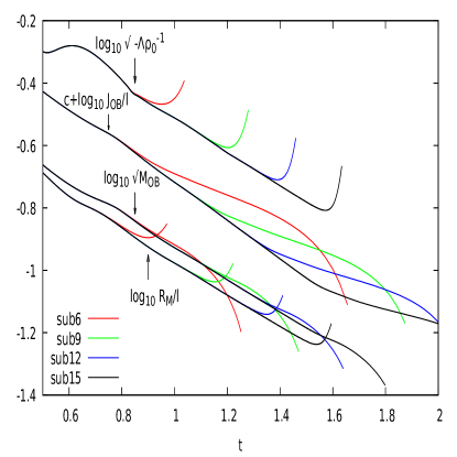
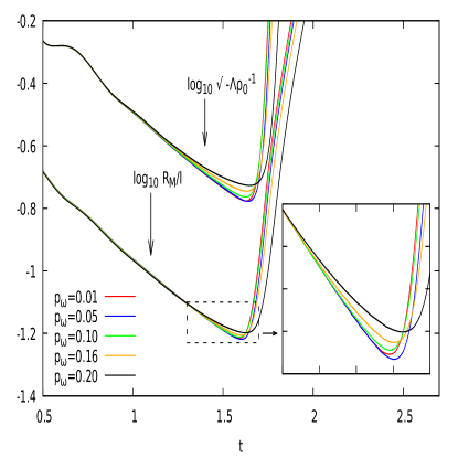
Figure 7: Left plot: lin-log plot of $R_{M}(t)/\ell$, $\sqrt{-\Lambda\rho_{0}^{-1}(t)}$, $\sqrt{M_{\text{OB}}(t)}$, and $J_{\text{OB}}(t)/\ell$ for sub6 to sub15 centered initial data with $p_{w}=0.01$, using the MC limiter. We observe that, as we fine-tune to the black-hole threshold, the solution approaches an intermediate attractor solution in which $R_{M}$, $\rho_{0}^{-1}$, $M_{\text{OB}}$ and $J_{\text{OB}}$ decrease exponentially. Less fine-tuned initial data peel off from this critical line sooner than more fine-tuned data, leading to critical scaling of the maximum density, etc. Note that $J_{\text{OB}}$ decreases more slowly than $M_{\text{OB}}$, as is the case for their values at the apparent horizon. There is a second regime for $J_{\text{OB}}$, after the critical regime, where it takes on another, less pronounced, power-law scaling. Right plot: lin-log plot of $\sqrt{-\Lambda\rho_{0}^{-1}(t)}$ and $\sqrt{R_{M}(t)/\ell}$ for our best subcritical (sub15) data with $p_{w}=0.01$, $0.05$, $0.1$, $0.16$, and $0.20$ using the Godunov limiter. At late times, these quantities decrease more slowly for larger $p_{w}$ and correspondingly larger spin-to-mass ratio.

In spherical symmetry, the critical solution is quasistatic, meaning that it adiabatically goes through the sequence of static solutions, with $s$ now a function of $t$, and $|\dot{s}(t)|\ll 1$. Furthermore, $\mu\sim s^{2}$, and it follows that in the quasistatic ansatz, $\mu(t)\sim s(t)^{2}$. Since the solution shrinks exponentially, we have the following ansatz for $s(t)$:

$$s(t)\equiv s_{0}e^{-\nu{t\over\ell}},$$ (41)

for constants $s_{0}$ and $\nu$. To leading order in $\dot{s}$, the quasistatic ansatz then takes the form

$$M(t,R)\simeq\check{M}\left({R\over s(t)};\mu(t),\tilde{\Omega}=0\right),$$ (42)

and similarly for other suitably rescaled variables.

As we hinted before, one can expect, at least in the regime where the effects of angular momentum are still perturbative, that the solution can be thought to shrink adiabatically to zero size, going through a sequence of stationary solutions. The picture in spherical symmetry can then be straightforwardly generalized to axisymmetric initial data. Specifically, we assume that, to leading order in $\dot{s}$, the critical solution can be well approximated by

$$M(t,R)\simeq\check{M}\left({R\over s(t)};\mu(t),\tilde{\Omega}(t)\right),$$ (43)

and so on. From the exponential form of $s(t)$, we further make a relatively agnostic ansatz for $\tilde{\Omega}$ of the form

$$\tilde{\Omega}(t)=:\tilde{\Omega}_{0}e^{-\phi{t\over\ell}},$$ (44)

where $\tilde{\Omega}_{0}$ and $\phi$ are constants. This exponential ansatz is justified from the fact that, for the family of stationary solutions, the angular momentum at infinity satisfies (39). In particular $J\sim\tilde{\Omega}$. From Fig. 7, $J_{\text{OB}}$, seen as a proxy for the corresponding angular momentum at infinity, decays exponentially, thus suggesting the exponential form for $\tilde{\Omega}$. Together with the ansatz for $s(t)$ (41), we have now four parameters to fit: $s_{0}$ and $\nu$ (as in spherical symmetry) and $\tilde{\Omega}_{0}$ and $\phi$.

For $p_{w}=0.01$, where we only observe type II behavior to our level of fine-tuning, we choose to fix them by requiring the central density and spin at infinity to match those of the stationary solutions at times $t\simeq 1.0$ and $1.4$, where we believe that the solution is in its critical regime; see Fig. 7. For the spin at infinity, we take the spin at the numerical outer boundary as a proxy. This is justified because in the atmosphere, where the density is small, the mass and spin are approximately constant in space. We find the following values:

$$s_{0} \simeq 0.1913,\qquad\nu\simeq 0.7925,$$

$$\tilde{\Omega}_{0} \simeq 0.002110,\quad\phi\simeq 0.1144.$$ (45)

As expected, the above values of $s_{0}$ and $\nu$ are consistent with their values in the spherically symmetric case $p_{w}=0$. We have repeated this procedure for the ingoing and off-centered initial data as well, and summarize the values of $\nu$ and $\phi$ in Table 1. Due to the smallness of $\phi$, the relative variation of $\phi$ is important. In particular, it is difficult to confidently say if those variations are purely a numerical error. However, because Figs. 5 and 6 suggest some universality for the critical solution, we are inclined to believe it is so. That is, we believe that $\phi$, just as $\nu$, is family independent. We find good agreement between the numerical and exact solutions.

Initial data ($\kappa=0.5$)	$\nu$	$\phi$
Off-centered	0.7844	0.0854
Centered	0.7925	0.1144
Ingoing	0.8049	0.0671

Table 1: The values of $\nu$ and $\phi$ for different families of initial data.

In Fig. 8, we compare the leading-order quasistationary solution for $J$, of the same form as in Eq. (43) (dotted lines), with the numerical data (solid lines) at constant time intervals $t\simeq 1$, $1.1$, $1.2$, $1.3$ and $1.4$.

Figure 8: Numerical solution (solid lines) for $J$, plotted against $R/s(t)$, at different times during the critical regime, $t\simeq 1$, $1.1$, $1.2$, $1.3$ and $1.4$ for our best subcritical, centered initial data with $p_{w}=0.01$. For comparison, we plot the leading-order term of the quasistationary solution for $J=\check{J}(R/s(t);\mu(t),\tilde{\Omega}(t))$ (dashed lines). We consider the ansatz $s(t)=s_{0}e^{-\nu t/\ell}$ and $\tilde{\Omega}(t)=\tilde{\Omega}_{0}e^{-\phi t/\ell}$, where the parameters $s_{0}$, $\nu$, $\tilde{\Omega}_{0}$, and $\phi$ are given in Eq. (45).

Returning back to the left plot of Fig. 7, the quasistationarity of the critical solution can be used to explain the slope of $J_{\text{OB}}$. Specifically, from (39), we have

$$J_{\text{OB}}\sim\tilde{\Omega}s.$$ (46)

In the spherically symmetric case, we showed that $M_{\text{OB}}\sim s^{2}$. At the level where angular momentum is still viewed as a perturbation, this is still expected to hold, so that

$$J_{\text{OB}}^{2}\sim\tilde{\Omega}^{2}M_{\text{OB}},$$ (47)

or

$$J_{\text{OB}}^{2}\sim M_{\text{OB}}^{1+\Delta},$$ (48)

where

$$\Delta=\phi/\nu$$ (49)

is small. For the centered initial data for example, (45) gives $\Delta\simeq 0.144$.

IV Conclusion

We have generalized our previous study [6] of perfect fluid critical collapse in $2+1$ spacetime dimension to rotating initial data. We have given evidence that, for $\kappa\lesssim 0.42$, the critical phenomena are type I, as in spherical symmetry. The critical solution is stationary and agrees well with the family of exact stationary solutions studied in another paper [11].

The situation for $\kappa\gtrsim 0.43$ is more complicated. We give evidence for the existence of a universal one-parameter family of critical solutions, which fibrates the region $|J/\ell|<M$, $M>0$ of the $J$-$M$ plane. In the limit $|J|/(\ell M)\ll 1$, as well as $s/\ell\ll 1$, angular momentum can be approximated as a linear perturbation of the nonrotating critical solution. We then expect both $s$ and $J$ to be exponential functions of $t$, and so $J$ to be a power of $s$.

However, for supercritical data, the angular momentum of the solution decreases more slowly than its mass as the black-hole threshold is approached. The spin-to-mass ratio therefore increases as we fine-tune to the black-hole threshold. We gave strong evidence that in the limit of perfect fine-tuning, the resulting black hole is extremal.

For small angular momentum, rotation can be treated as a linear perturbation of spherical symmetry. The universality of the one-parameter family of critical solutions, with increasing $|J|/(\ell M)$, then implies the existence of a single unstable rotating mode of the spherical critical solution. One may then wonder how superextremality is avoided. We have seen that the answer is that the critical solution stops shrinking as $|J|/(\ell M)\to 1$, and so both $J$ and $M$ stop scaling.

Contrast this with the known situation in rotating fluid collapse in $3+1$ [13, 14]. There, the existence of a single growing angular momentum mode is known for $\kappa<1/9$ [15], but it turns out that nonlinear effects make $J/M^{2}$ decrease in the critical solution from the start, even for small $J$ for $\kappa<1/9$.

As $s/\ell\ll 1$, or $M\ll 1$, the physics become approximately scale invariant, and the cosmological constant becomes essential only in a boundary layer at the surface of the contracting star. We expect that in this limit the one-parameter family of critical solutions degenerates to a single (somewhat singular) critical solution, up to an overall rescaling.

We have shown that type I critical collapse is controlled by rigidly rotating stationary solutions and type II by an adiabatic shrinking sequence of such solutions. The matching between our numerical results and the exact stationary solutions of [11] is very good, even neglecting the adiabatic contraction. On the flip side, we have not been able to derive effective adiabatic equations of motion in the space of stationary solutions (even in the nonrotating case of [6]), and so we are unable to derive either the universal time dependence of the critical solutions or their unique trajectories in the $J$-$M$ plane.

It is fortunate that our critical solutions appear to be exactly rigidly rotating, as precisely all rigidly rotating stationary solutions are known in closed form (for arbitrary equation of state) [11, 12]. It is plausible that the rigid rotation of the critical solutions is universal, but we have not tested this, as we have considered only one family of initial rotation profiles (in which the angular velocity is approximately constant).

Critical phenomena in $2+1$ dimensions primarily serves as toy model which makes the transition from spherical to axisymmetric initial data, unlike the $3+1$ dimensional setting, much more tractable. Between the results from the scalar field case [8, 5] and the results for the perfect fluid here, one can see that the effects of angular momentum are generally far from trivial and share little resemblance with their higher-dimensional counterparts.

- [1] M. W. Choptuik, Universality and Scaling in Gravitational Collapse of a Massless Scalar Field, Phys. Rev. Lett. 70, 9 (1993).
- [2] C. Gundlach and J. M. Martin-García, Critical phenomena in gravitational collapse, Living Rev. Relativity 10, 5 (2007).
- [3] A. M. Abrahams and C. R. Evans, Critical Behavior and Scaling in Vacuum Axisymmetric Gravitational Collapse, Phys. Rev. Lett. 70, 2980 (1993).
- [4] M. Bañados, C. Teitelboim, and Jorge Zanelli, Black Hole in Three-Dimensional Spacetime, Phys. Rev. Lett. 69, 13 (1992).
- [5] J. Jałmużna and C. Gundlach, Critical collapse of a rotating scalar field in dimensions, Phys. Rev. D 95, 084001 (2017).
- [6] P. Bourg and C. Gundlach, collapse of spherically symmetric perfect fluid, Phys. Rev. D 103, 124055 (2021).
- [7] F. Pretorius and M. W. Choptuik, Gravitational collapse in dimensional AdS spacetime, Phys. Rev. D. 62, 12 (2000).
- [8] J. Jałmużna, C. Gundlach, and T. Chmaj, Scalar field critical collapse in dimensions, Phys. Rev. D 92, 12 (2015).
- [9] C. Gundlach, P. Bourg, and A. Davey, A fully constrained, high-resolution shock-capturing, formulation of the Einstein-fluid equations in dimensions, Phys. Rev. D 104, 024061 (2021).
- [10] S. Kinoshita, Extension of Kodama vector and quasilocal quantities in three-dimensional axisymmetric spacetimes, Phys. Rev. D 103, 124042 (2021).
- [11] C. Gundlach and P. Bourg, Rigidly rotating perfect fluid stars in dimensions, Phys. Rev. D 102, 084023 (2020).
- [12] M. Cataldo, Rotating perfect fluids in (2+1)-dimensional Einstein gravity, Phys. Rev. D 69, 064015 (2004).
- [13] T.W. Baumgarte and C. Gundlach, Critical Collapse of Rotating Radiation Fluid, Phys. Rev. Lett. 116, 22 (2016).
- [14] C. Gundlach and T.W. Baumgarte, Critical gravitational collapse with angular momentum. II. Soft equations of state, Phys. Rev. D 97, 06 (2018).
- [15] C. Gundlach, Critical gravitational collapse of a perfect fluid: Nonspherical perturbations, Phys. Rev. D 65, 8 (2002).