Image reconstruction in light-sheet microscopy: spatially varying deconvolution and mixed noise

Abstract

We study the problem of deconvolution for light-sheet microscopy, where the data is corrupted by spatially varying blur and a combination of Poisson and Gaussian noise. The spatial variation of the point spread function (PSF) of a light-sheet microscope is determined by the interaction between the excitation sheet and the detection objective PSF. First, we introduce a model of the image formation process that incorporates this interaction, therefore capturing the main characteristics of this imaging modality. Then, we formulate a variational model that accounts for the combination of Poisson and Gaussian noise through a data fidelity term consisting of the infimal convolution of the single noise fidelities, first introduced in [1]. We establish convergence rates in a Bregman distance under a source condition for the infimal convolution fidelity and a discrepancy principle for choosing the value of the regularisation parameter. The inverse problem is solved by applying the primal-dual hybrid gradient (PDHG) algorithm in a novel way. Finally, numerical experiments performed on both simulated and real data show superior reconstruction results in comparison with other methods.

1 Introduction

Light-sheet microscopy is a fluorescence microscopy technique that enables volumetric imaging of biological samples at high frame rate with better sectioning and lower photo-toxicity in comparison to other fluorescent techniques. This is achieved by illuminating a thin slice of the sample using a sheet of light and detecting the emitted fluorescence from this plane with another objective perpendicular to the plane of the sheet. A schematic representation of a light-sheet microscope is shown in Figure 1. By contrast, widefield microscopy illuminates the whole sample using a single objective and achieves only very limited sectioning. Confocal microscopy allows improved sectioning by utilising a pinhole to discard out-of-focus light, at the cost of higher photo-toxicity and reduced frame rate. By only selectively illuminating the slice of the sample being imaged, less photo-toxicity damage is induced in light-sheet microscopy and, therefore, imaging of living samples over a longer period of time is possible. The combination of lower photo-toxicity, better sectioning capabilities and faster image acquisition led to light-sheet microscopy being recognised as “Method of the Year” by Nature Methods in 2014 [2].

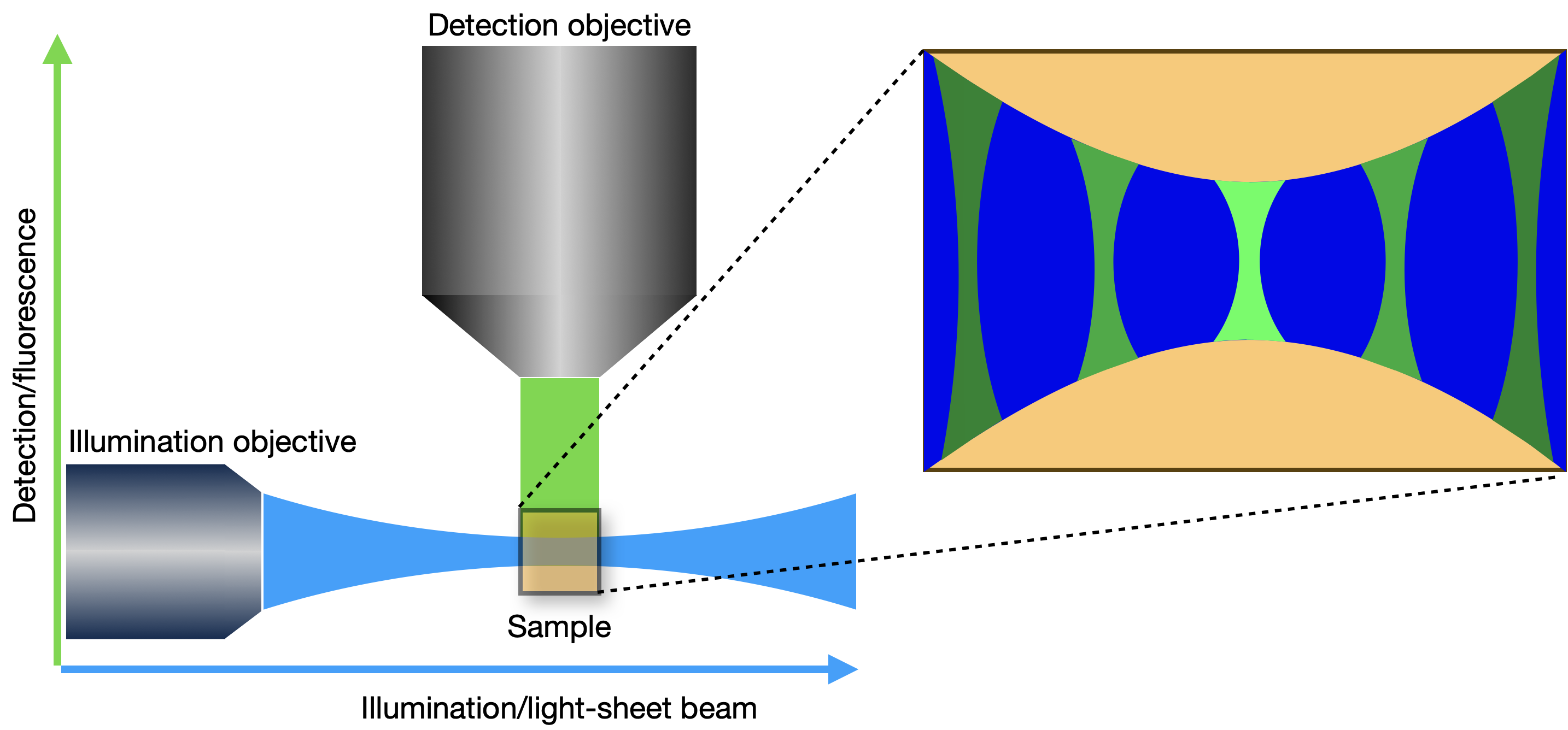
Figure 1: Schematic of a light-sheet microscope, showing the illumination and the detection directions. The interaction of the light-sheet with the detection PSF leads to a spatially varying overall PSF and decreasing of the pixel intensities away from the centre in the horizontal direction.

The focus of the present manuscript is on deconvolution techniques for light-sheet microscopy data. In this context, deconvolution refers to the computational method of reversing the effect of blurring in the image acquisition process due to the point spread function (PSF) of the microscope [3, 4, 5]. Specifically, the PSF of an imaging system represents its response to a point object. Knowledge of the PSF, which can be modelled mathematically and calibrated using bead data (samples containing small spheres of known dimensions), is used in the formulation of a forward model of the image formation, which can then be inverted, for example using optimisation methods, to reconstruct the original, deblurred object [6].

In the case of light-sheet microscopy, simply knowing or estimating the PSF of the detection objective is not sufficient, since the overall response of the system to a point source is also influenced by the excitation light-sheet used to illuminate the slice. The overall PSF could be approximated by the detection PSF in the region where the illumination sheet is focused. However, the detection PSF becomes more distorted and loses intensity away from the focus of the excitation light-sheet, which is illustrated in Figure 1. Therefore, the problem we propose to address can be seen as a specific case of spatially-varying deconvolution [7, 8].

Two examples of acquired data are shown in Figure 2. We can see in both cases the effect of the spatially varying light-sheet: the image is sharper in the centre and blurry on the sides, with the amount of blur growing with the horizontal distance from the centre. In addition, the fluorescence intensity of imaged beads in Figure 2(a) is unevenly distributed despite imaging a homogeneous sample of beads, with the centre of the image being brighter than the left and right sides. The aim of our work is to correct these effects.

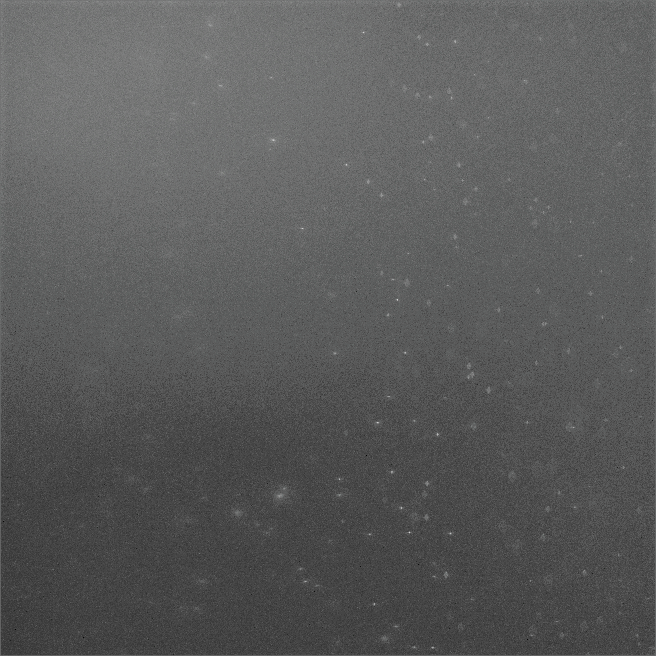
(a) $0.5\mu m$ multi-colour Tetraspeck microspheres (slice)

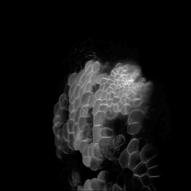
(b) Membrane labelled Marchantia thallus (maximum intensity projection)

Figure 2: Examples of light-sheet microscopy data of dimensions $665.6\mu m\times 665.6\mu m$: beads in (a) and Marchantia thallus in (b). The effect of the light-sheet is visible along the horizontal direction, as the image is sharp in the centre, where the sheet is focused, while the quality of the image decreases away from the centre. Another source of blur observed, especially in the bead image (left) is given by optical aberrations due to the sample imaging medium (dynamic range is stretched for better visibility). The Marchantia image has been acquired using samples from Dr. Alessandra Bonfanti and Dr. Sarah Robinson using the genetic line provided by Prof. Sebastian Schornack and Dr. Giulia Arsuffi at the Sainsbury Laboratory Cambridge University.

1.1 Contribution

We propose a method for deconvolution of 3D light-sheet microscopy data that takes into account the spatially varying nature of the PSF and is scalable to the dimensions typical to biological samples imaged using light-sheet microscopy – 4.86GB per 3D 16-bit stack of $2048\times 2048\times 580$ voxels.

Our approach is based on a new model for image formation that describes the interaction between the light-sheet and the detection PSF which replicates the physics of the microscope. Then, we formulate an inverse problem where the forward operator is given by model of the image formation process and which takes into account the degradation of the data by both Gaussian and Poisson noise as an infimal convolution between an $\operatorname{\mathrm{L}}^{2}$ term and a Kullback-Leibler divergence term, following [1]. The proposed variational problem is solved by applying the Primal Dual Hybrid Gradient (PDHG) algorithm in a novel way. Finally, we exploit the noise model to automatically tune the balance between the data fidelity and regularisation resorting to a discrepancy principle. We obtain convergence rates in a Bregman distance for the infimal convolution fidelity from [1] under a standard source condition.

In our numerical experiments, we first show how this method performs on simulated data, where the ground truth is known, then we apply our method to two examples of data from experiments: an image of fluorescent beads and a sample of Marchantia. In both cases, we see that the deconvolved images show improved contrast, while outperforming deconvolution using only the constant detection PSF.

1.2 Related work

Before describing in more detail our approach to the deconvolution problem, we give a brief overview of the literature on spatially varying deconvolution in the context of microscopy and how our work relates to it.

Purely data-driven approaches estimate a spatially varying PSF in a low dimensional space (for scalability reasons) using bead images [9, 7, 8]. This is usually not application specific and can be included in a more general blind deconvolution framework. Similarly, the work in [10] involves writing the spatially varying PSF as a convex combination of spatially invariant PSFs. The algorithm alternates between estimating the image and estimating the PSF. In a similar vein, the authors of [11] approach the problem of blind deconvolution by defining the convolution operator using efficient matrix-vector multiplication operations. This decomposition is similar to the discrete formulation of our image formation model. These methods optimise over the (unknown) operator in addition to the unknown image. Related to these results is [12], where the authors consider the models from [9] and [11] under the assumption that the blurring operator is known and given as a sum of weighted spatially invariant operators. They exploit this structure of the operator and use a Douglas-Rachford based splitting to solve the optimisation problem efficiently. While more general than our approach, we consider that using the knowledge of the image formation process in the forward model is advantageous for the reconstruction of light-sheet microscopy data.

A number of groups consider the problem of reconstruction from multiple views in the context of light-sheet microscopy. In [13], the problem of multi-view reconstruction under a spatially varying blurring operator for 3D light-sheet data is considered. They divide the image into small blocks where they perform deconvolution using spatially-invariant PSFs estimated from beads (and interpolated PSFs in regions where there are no beads). In [14], the authors extend the Richardson-Lucy algorithm to the multi-view reconstruction problem in a Bayesian setting. While it allows for different PSFs for each view (estimated using beads), this work does not consider spatial variations of the PSF. While using data from multiple views improves the quality of the reconstruction, these approaches are agnostic to the physics of the microscope.

Taking an approach similar in spirit to ours, the authors of [15] model the effective PSF of a light-sheet microscope, which is then plugged into a regularised version of the Richardson-Lucy algorithm for deconvolution. However, while they model the detection PSF and the light-sheet separately, they assume the effective PSF of the microscope is spatially invariant and the point-wise product of the two PSFs. In contrast, we do not take this simplifying step in our modelling, as we consider that the relationship between the two PSFs plays in important role in the resulting blur of the image.

The work of Guo et al. in [16] uses a modified Richardson-Lucy algorithm implemented on GPU to improve the speed of convergence, further improved by the use of a deep neural network, which is a promising approach.

Moreover, in [17] the authors introduce an image formation model similar to the one described in the present manuscript. However, the regions of the resulting PSF where the light-sheet is out of focus are discarded, hence approximating the overall PSF with a constant PSF and then performing deconvolution using the ADMM algorithm. In Cueva et al. [18], a mathematical model which takes into account image fusion with two sided illumination is derived from fist principles. However, it is restricted to 2D and they do not apply the method to real data.

Lastly, regarding the mixed Gaussian-Poisson noise fidelity, our method follows the infimal convolution variational approach described in [1], with the additional light-sheet blurring operator. The same inverse problem, without the blurring operator, is solved in [19] albeit using an ADMM algorithm for the minimisation.

1.3 Paper structure

The paper is organised as follows. In Section 2, we introduce a mathematical model of the image formation process in a light-sheet microscope. This model describes how the sample is blurred by the excitation illumination together with the detection objective PSF. Optical aberrations of the system are modelled using Zernike polynomials in the detection PSF, which we discuss in Section 2.3. In Section 3, we define the mathematical setting for the deconvolution problem and we state an inverse problem using a data fidelity as an infimal convolution of the individual Gaussian and Poisson data fidelities. We discuss convergence rates and a discrepancy principle for choosing the regularisation parameter in Section 2.1. In Section 4, we describe how PDHG is applied to this inverse problem, with details of the implementation of the proximal operator and the convex conjugate of the joint Kullback-Leibler divergence. Finally, we validate our method with numerical experiments both with simulated and real data in Section 5, before concluding and giving a few directions for future work in Section 6.

2 Forward model

The first contribution of the current work is a model of the image formation process in light-sheet microscopy. By modelling the excitation light-sheet and the detection PSF separately and their interaction in a way that replicates the physics of the microscope, we are able to accurately simulate the spatially varying PSF of the imaging system. We then incorporate this knowledge as the forward model in an inverse problem, which we solve to remove the noise and blur in light-sheet microscopy data. In this section, we describe the image formation process and the PSF model.

2.1 Image formation model

A light-sheet propagated along the $x$ direction is focused by the excitation objective at an axial position $z=z_{0}$ and the local light-sheet intensity $l$ is modelled by the incoherent point spread function (PSF) of the excitation objective. The sample with local density of fluorophores $u$ emits photons proportionally to the local intensity $l$ of the light-sheet. These photons are then collected by a detection objective, whose action on the illuminated sample is modelled as a convolution with its PSF $h$. Finally, the sensor conjugated with the image plane $z_{0}$ collects photons and converts them to digital values for storage. Consequently, the recorded image is corrupted by a combination of Gaussian and Poisson noise. We can see here again how the local variation of the light-sheet will result into a spatially varying blur and spatially-varying illumination intensity in the captured image. This process is then repeated for each $z_{0}$ to obtain the measured data $f$.

More specifically, we model $u$, $f$, $l$ and $h$ as functions defined on $\Omega\subset\mathbb{R}^{3}$, a rectangular domain of dimensions $\Omega_{x}\times\Omega_{y}\times\Omega_{z}$ (in $\mu m$) with $\Omega=[-\frac{\Omega_{x}}{2},\frac{\Omega_{x}}{2}]\times[-\frac{\Omega_{y}}{2},\frac{\Omega_{y}}{2}]\times[-\frac{\Omega_{z}}{2},\frac{\Omega_{z}}{2}]$. For the sample $u$, the light-sheet $l$ and the detection objective PSF $h$, the measured data $f$ is given by:

$$f(x,y,z)=\iiint l(s,t,w)u(s,t,w-z)h(x-s,y-t,w)\operatorname{d\!}s\operatorname{d\!}t\operatorname{d\!}w.$$ (2.1)

The detection PSF $h$ is given by

$$h(x,y,z)=\left|\iint g_{\sigma}*p_{Z}(\kappa_{x},\kappa_{y})e^{2i\pi z\sqrt{(n/\lambda_{h})^{2}-\kappa_{x}^{2}-\kappa_{y}^{2}}}e^{2i\pi(\kappa_{x}x+\kappa_{y}y)}\operatorname{d\!}\kappa_{x}\operatorname{d\!}\kappa_{y}\right|^{2}$$ (2.2)

and the light-sheet $l$ is the y-averaged light-sheet beam PSF $l_{beam}$:

$$l_{beam}(x,y,z)=\left|\iint p_{0}(\kappa_{z},\kappa_{y})e^{2i\pi x\sqrt{(n/\lambda_{l})^{2}-\kappa_{z}^{2}-\kappa_{y}^{2}}}e^{2i\pi(\kappa_{z}z+\kappa_{y}y)}\operatorname{d\!}\kappa_{z}\operatorname{d\!}\kappa_{y}\right|^{2},$$ (2.3)

where $n$ is the refractive index, $\lambda_{h},\lambda_{l}$ are the wave lengths corresponding to the detection objective and light-sheet beam respectively, and $g_{\sigma}$ represents Gaussian blur. Lastly, $p_{Z}(\kappa_{x},\kappa_{y})$ and $p_{0}(\kappa_{z},\kappa_{y})$ are the pupil functions for the detection PSF and the light-sheet beam respectively, both given by:

$$p_{\varphi}(x,y)=\begin{cases}e^{2i\pi\varphi}\quad&\text{for}\quad\sqrt{x^{2}+y^{2}}\leqslant NA/\lambda_{i},\\ 0\quad&\text{otherwise},\end{cases}$$ (2.4)

for their respective $\lambda_{i}=\lambda_{h}$ or $\lambda_{i}=\lambda_{l}$, where the phase for the light-sheet pupil $p_{0}$ is equal to zero and the phase for the detection PSF pupil $p_{Z}$ is an approximation of the optical aberrations written as an expansion in a Zernike polynomial basis, which we will explain in more detail in Section 2.3, and with different numerical apertures NA. In general, the NA of the excitation sheet is much lower than the NA of the detection lens. We note that the overall process is not translation invariant and cannot be modelled by a convolution operator.

Note that both the detection PSF $h$ and the light-sheet PSF have a similar formulation derived from:

$$\text{PSF}(x,y,z)=\left|\iint p(\kappa_{x},\kappa_{y})e^{2i\pi z\sqrt{(n/\lambda_{i})^{2}-\kappa_{x}^{2}-\kappa_{y}^{2}}}e^{2i\pi(\kappa_{x}x+\kappa_{y}y)}\operatorname{d\!}\kappa_{x}\operatorname{d\!}\kappa_{y}\right|^{2},$$ (2.5)

which includes the pupil function for modelling aberrations and a defocus term before taking the Fourier transform (see, for example [20, 21]).

In practice, the image formation process modelled by (2.1) is discretised at the point of recording by the camera sensor in the $xy$ plane and by the step size of the light-sheet in the $z$ direction. If the camera has a resolution of $N_{x}\times N_{y}$ pixels and the light-sheet illuminates the sample at $N_{z}$ distinct steps, the model (2.1) becomes:

$$\tilde{f}_{i,j,k}=\frac{1}{\tilde{C}}\sum_{i^{\prime}=1}^{N_{x}}\sum_{j^{\prime}=1}^{N_{y}}\sum_{k^{\prime}=1}^{N_{z}}\tilde{l}_{i^{\prime},j^{\prime},k^{\prime}}\tilde{u}_{i^{\prime},j^{\prime},k^{\prime}-k}\tilde{h}_{i-i^{\prime},j-j^{\prime},k^{\prime}},$$ (2.6)

for all $i=1,\ldots,N_{x},j=1,\ldots,N_{y},k=1,\ldots,N_{z}$, and a normalisation constant $\tilde{C}$, where $\tilde{u},\tilde{f},\tilde{l},\tilde{h}\in\mathbb{R}^{N_{x}\times N_{y}\times N_{z}}$ are the discretised versions of $u,f,l,h$ respectively. Similarly, the sampling performed by the camera sensor leads to a discretisation of the Fourier space and the use of the discrete Fourier transform in the PSF and light-sheet models (2.2) and (2.3). Lastly, in our implementation we normalise $\tilde{h}$ so that $\sum_{i=1}^{N_{x}}\sum_{j=1}^{N_{y}}\sum_{k=1}^{N_{z}}\tilde{h}_{i,j,k}=1$ and choose the normalisation constant $\tilde{C}$ so that the norm of the resulting operator is equal to one.

2.2 Derivation of the model

Let $l,u,h$ be defined as in Section 2.1, with $h$ symmetric around the origin and $l$ translation invariant in the $y$ direction, centred and symmetric in the $xz$ plane around the origin. For a fixed $z_{0}\in[-\frac{\Omega_{z}}{2},\frac{\Omega_{z}}{2}]$, we take the following steps, which replicate the inner workings of a light-sheet microscope:

1. Image the sample at $z=z_{0}$: centre the sample $u$ at $z_{0}$ and multiply the result with the light-sheet $l$:

   $$F(x,y,z;z_{0})=l(x,y,z)\cdot u(x,y,z-z_{0}),$$ (2.7)

2. Convolve with the objective PSF $h$:

   $$C(x,y,z;z_{0}) =F(x,y,z;z_{0})*h(x,y,z)$$ (2.8)

   $$=\iiint F(s,t,w;z_{0})h(x-s,y-t,z-w)\operatorname{d\!}s\operatorname{d\!}t\operatorname{d\!}w$$ (2.9)

3. Slice at $z=0$:

   $$f(x,y,z_{0})=\left[C(x,y,z;z_{0})\right]_{z=0},$$ (2.10)

which leads to:

$$f(x,y,z_{0})=\iiint l(s,t,w)u(s,t,w-z_{0})h(x-s,y-t,-w)\operatorname{d\!}s\operatorname{d\!}t\operatorname{d\!}w.$$ (2.11)

This is the same as model (2.1), where we substitute $z$ for $z_{0}$ and note that $h$ is symmetric in the third variable around the origin.

For a discretisation of the domain using a 3D grid with $N_{x}\times N_{y}$ pixels and $N_{z}$ light-sheet steps, the forward model can be computed by following the three steps above for each $k=1,\ldots,N_{z}$, where we perform the convolutions using the fast Fourier transform (FFT), resulting in a number of $\mathcal{O}(N_{x}N_{y}N_{z}^{2}\log(N_{x}N_{y}N_{z}))$ operations.

Alternatively, we can re-write the last integral above as:

$$f(x,y,z_{0})=\int K(x,y,w)*h(x,y,w)\operatorname{d\!}w,$$ (2.12)

where

$$K(x,y,w)=l(x,y,w)u(x,y,w-z_{0}),$$ (2.13)

and the convolution in (2.12) is a 2D convolution in $(x,y)$:

$$K(x,y,w)*h(x,y,w)=\iint K(s,t,w)h(x-s,y-t,w)\operatorname{d\!}s\operatorname{d\!}t.$$ (2.14)

In terms of numbers of FFTs performed on a discretised $N_{x}\times N_{y}\times N_{z}$ grid, this alternative formulation requires $\mathcal{O}(N_{x}N_{y}N_{z}^{2}\log(N_{x}N_{y}))$ operations.

2.3 Point spread function model

While both the light-sheet profile and the detection PSF are based on the same model of a defocused system (2.5) introduced in [20], note that our definition of $h$ in (2.2) includes an additional convolution operation with a Gaussian $g_{\sigma}$ and a pupil function $p_{Z}$ with a non-zero phase. Let us turn to why this is the case.

It is well known that optical aberrations hamper results based on deconvolution with theoretical PSFs. In light-sheet microscopy, the effect of aberrations is more visible away from the centre, as shown for example in the bead image in Figure 2, or in the more detailed example beads in Figure 3. It is, therefore, required that we model the (spatially invariant) aberrations of the detection lens.

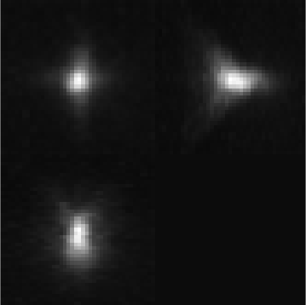
(a) Bead, no aberrations (maximum intensity projections)

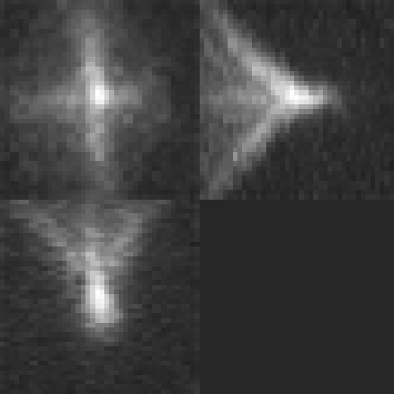
(b) Bead, with aberrations (maximum intensity projections)

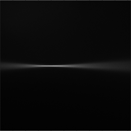
(c) Light sheet profile (slice showing an $x-z$ plane)

Figure 3: Examples of beads and light-sheet profile. The bead in (a) is cropped from the centre of Figure 2(a) and the bead in (b) is cropped from the right-hand side of Figure 2(a). The maximum intensity projections are taken in the $x-y$ plane (top left), the $z-y$ plane (top right) and the $x-z$ plane (bottom left).

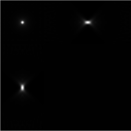
Figure 4: Objective PSF used in our model, with no aberrations (maximum intensity projections taken in the same way as in Figure 3).

The general PSF model (2.5), with the phase of the pupil function equal to zero, does not take optical aberrations into account and therefore it is not an accurate representation of the objective PSF $h$. For example, a PSF calculated using (2.5) with zero phase of the pupil and the parameters of the detection objective, shown in Figure 4, does not resemble the actual bead images in the data in Figure 3.

There has been extensive work on the problem of phase reconstruction in the literature [22, 23, 24, 25], but here we take a more straightforward approach using Zernike polynomials to include aberrations in the PSF [26], as follows. Let $h_{z}$ be the objective PSF calculated using (2.5) with Zernike polynomials in the phase of the pupil function:

$$h_{z}(x,y,z;c)=\left|\iint p_{Z}(\kappa_{x},\kappa_{y};c)e^{2i\pi z\sqrt{(n/\lambda_{h})^{2}-\kappa_{x}^{2}-\kappa_{y}^{2}}}e^{2i\pi(\kappa_{x}x+\kappa_{y}y)}\operatorname{d\!}\kappa_{x}\operatorname{d\!}\kappa_{y}\right|^{2},$$ (2.15)

where $p_{z}(\kappa_{x},\kappa_{y};c)$ is the pupil function with Zernike polynomials in the phase:

$$p_{z}(\kappa_{x},\kappa_{y};c)=\begin{cases}e^{2i\pi\sum_{j=1}^{15}c_{j}Z_{j}(\kappa_{x},\kappa_{y})}&\text{for}\quad\rho=\sqrt{\kappa_{x}^{2}+\kappa_{y}^{2}}\leqslant NA/\lambda_{h},\\ 0,\quad&\text{otherwise,}\end{cases}$$ (2.16)

and $c=[c_{1},\ldots,c_{15}]^{T}$ are coefficients corresponding to the polynomials. The Zernike polynomials and the corresponding coefficients that we use are given in Table 1 and shown in Figure 5.

Moreover, let $h_{zb}$ be the blurred PSF obtained by convolving $h_{z}$ with a Gaussian $g_{\sigma}$ with width $\sigma$:

$$h_{zb}(x,y,z;c,\sigma)=h_{z}(x,y,z;c)*g_{\sigma}.$$ (2.17)

This allows us to obtain a better approximation of the objective PSF. The parameters $c$ and $\sigma$ are calculated by solving the least-squares problem

$$\min_{c,\sigma}\|h_{zb}(c,\sigma)*b-h_{bead}\|_{2}^{2}\quad\text{subject to}\quad c\in[-3,3]^{15},\sigma>0,$$ (2.18)

where $h_{bead}$ is the bead image from Figure 3b and $b$ is equal to one inside the sphere of the radius equal to the radius of the bead (a parameter that is provided) and zero outside the sphere. This takes into account the non-negligible size of the beads used to generate the data.

In the implementation of the fitting procedure, we normalise both the bead image $h_{bead}$ and the simulated PSF $h_{zb}$ by their maximum values before calculating their error, and we include two additional parameters, scaling and shift, to ensure a better fit of the intensity values (not shown here for simplicity of the presentation). The resulting PSF is the detection PSF model (2.2) and is shown in Figure 6.

$Z_{j}$	Polynomial	$c_{j}$
$Z_{1}$	$\rho\cos\theta$	-0.7763
$Z_{2}$	$\rho\sin\theta$	-0.0460
$Z_{3}$	$2\rho^{2}-1$	-2.3608
$Z_{4}$	$\rho^{2}\cos 2\theta$	-1.3001
$Z_{5}$	$\rho^{2}\sin 2\theta$	0.2024
$Z_{6}$	$(3\rho^{2}-2)\rho\cos\theta$	-0.3999
$Z_{7}$	$(3\rho^{2}-2)\rho\sin\theta$	0.0348
$Z_{8}$	$6\rho^{4}-6\rho^{2}+1$	-1.2112
$Z_{9}$	$\rho^{3}\cos 3\theta$	-0.1521
$Z_{10}$	$\rho^{3}\sin 3\theta$	-0.0466
$Z_{11}$	$(4\rho^{2}-3)\rho^{2}\cos 2\theta$	-0.0930
$Z_{12}$	$(4\rho^{2}-3)\rho^{2}\sin 2\theta$	0.0427
$Z_{13}$	$(10\rho^{4}-12\rho^{2}+3)\rho\cos\theta$	-0.0117
$Z_{14}$	$(10\rho^{4}-12\rho^{2}+3)\rho\sin\theta$	-0.0581
$Z_{15}$	$20\rho^{6}-30\rho^{4}+12\rho^{2}-1$	-0.0633

Table 1: The first 15 Zernike Polynomials (in polar coordinates) and their coefficients used in $h_{z}$.

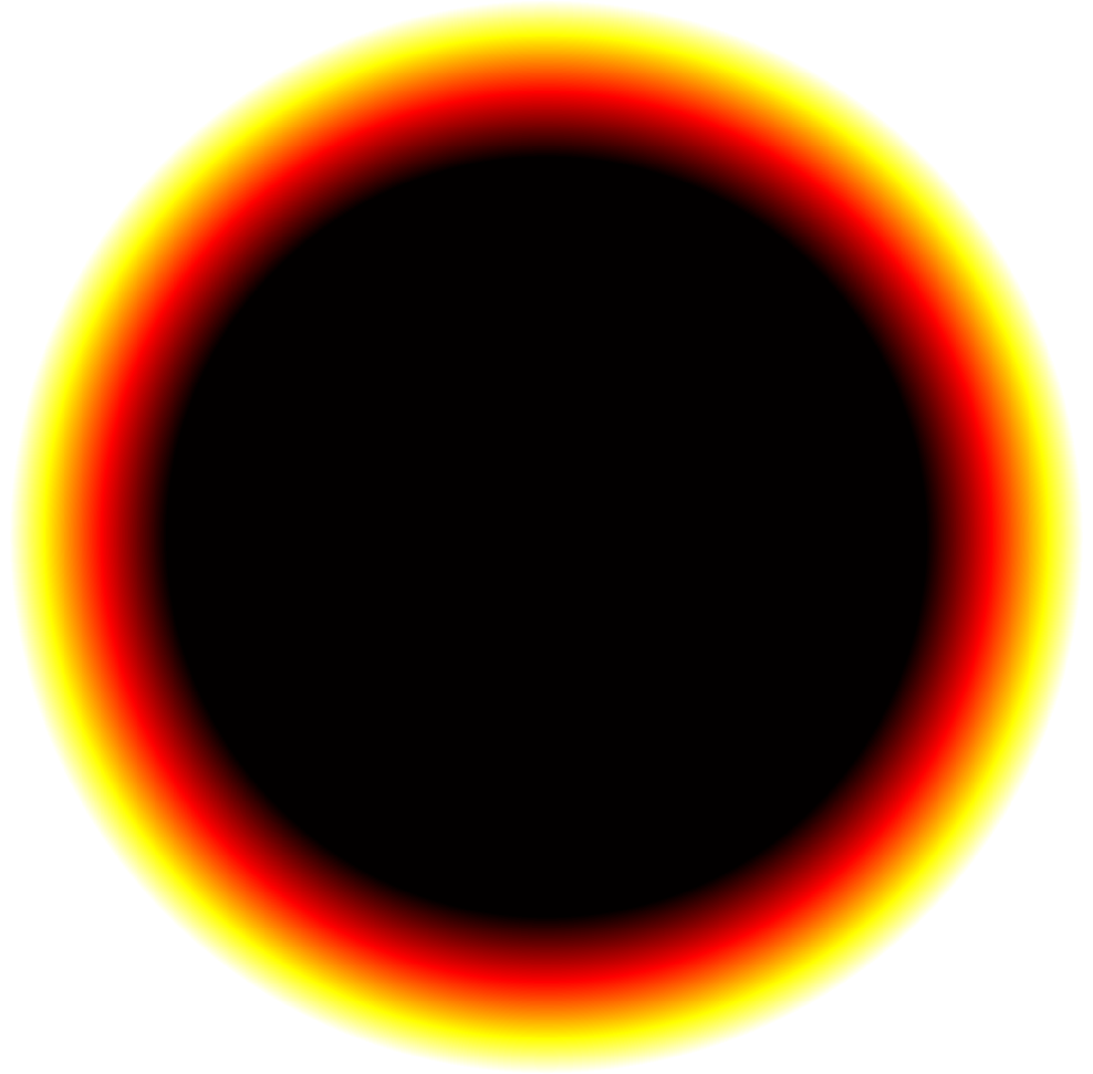
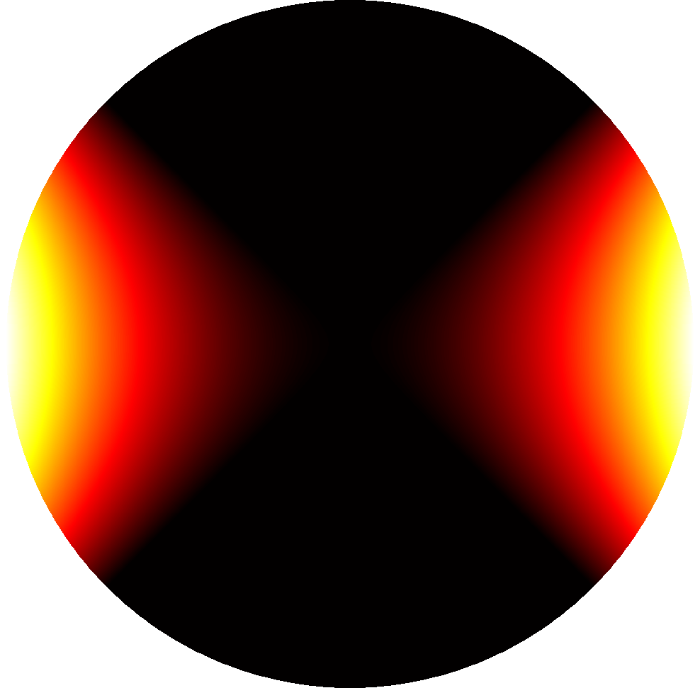
$Z_{1}$	$Z_{2}$	$Z_{3}$	$Z_{4}$
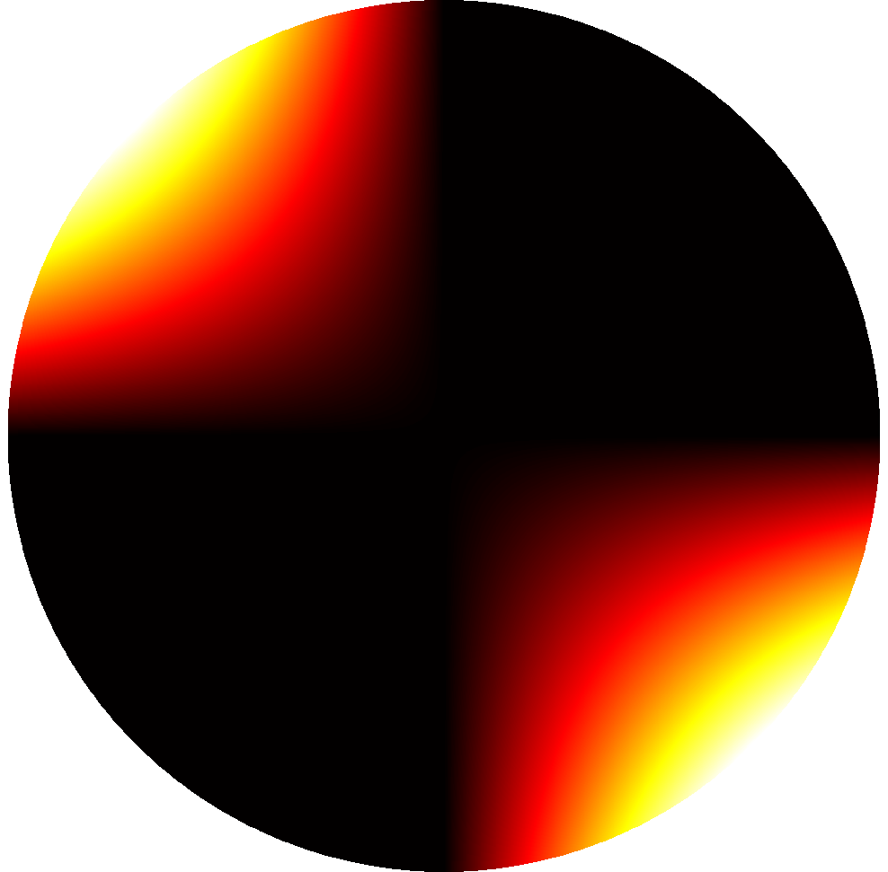
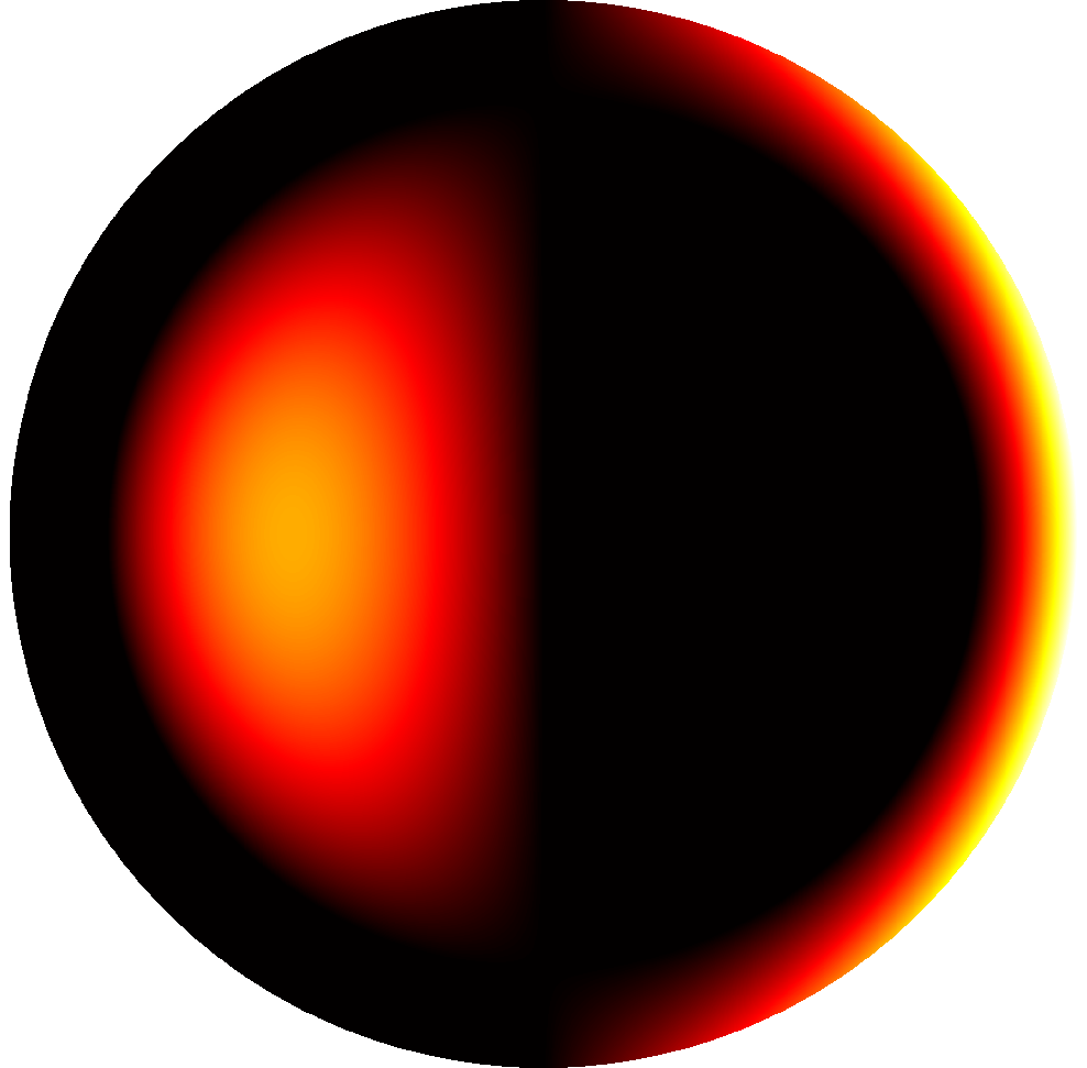
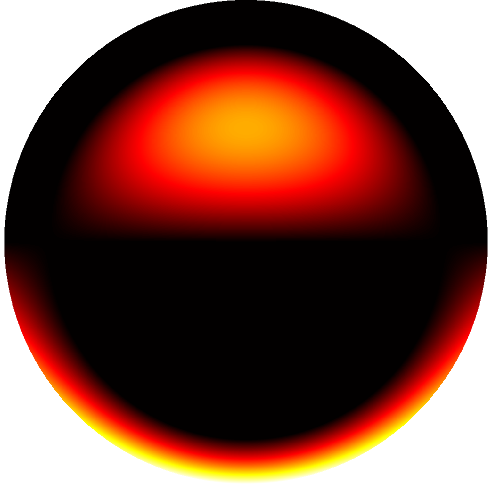
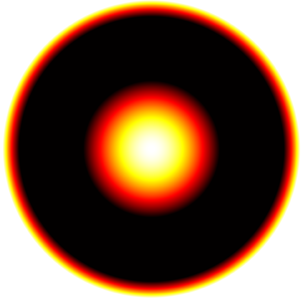
$Z_{5}$	$Z_{6}$	$Z_{7}$	$Z_{8}$
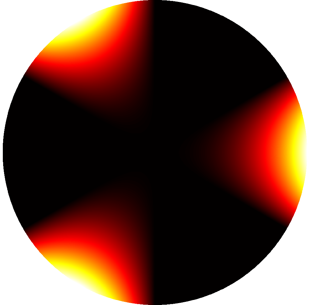
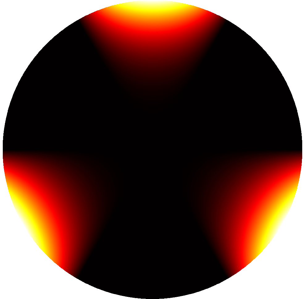
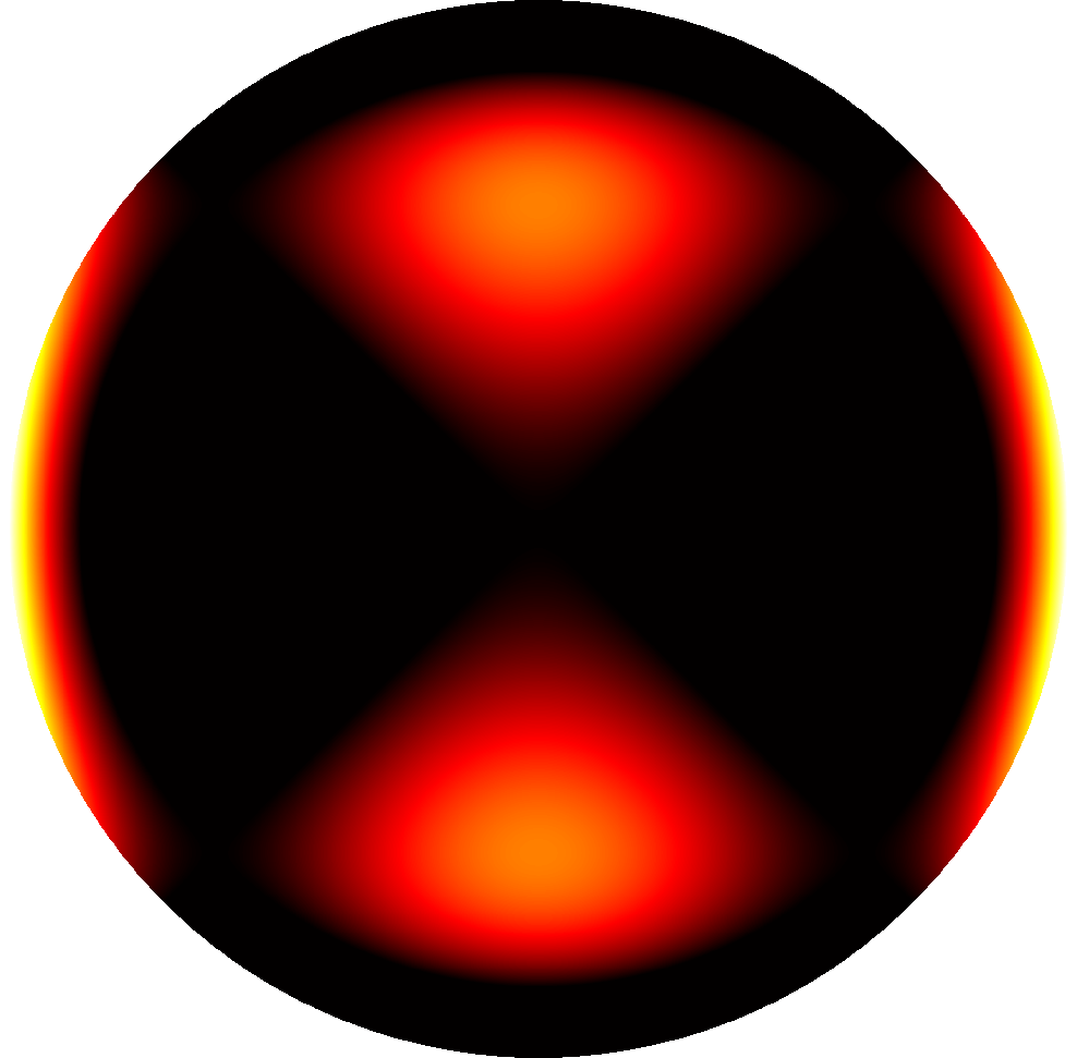
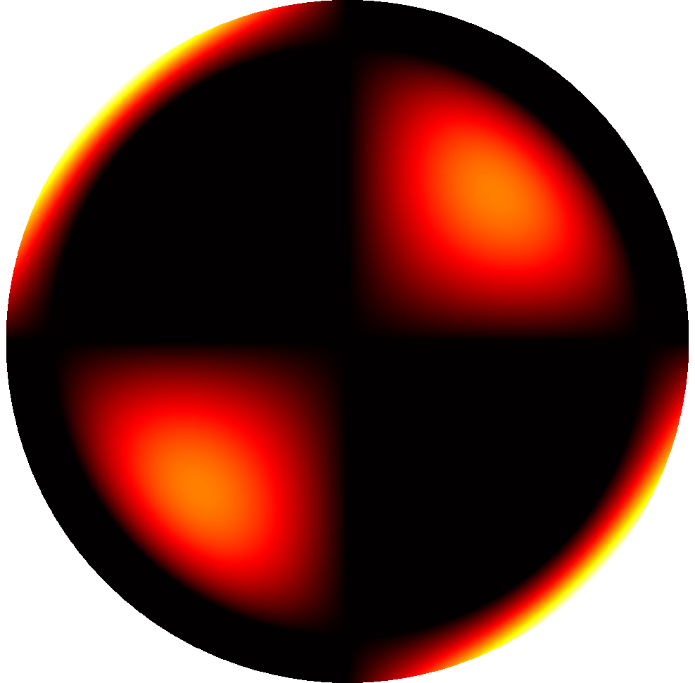
$Z_{9}$	$Z_{10}$	$Z_{11}$	$Z_{12}$
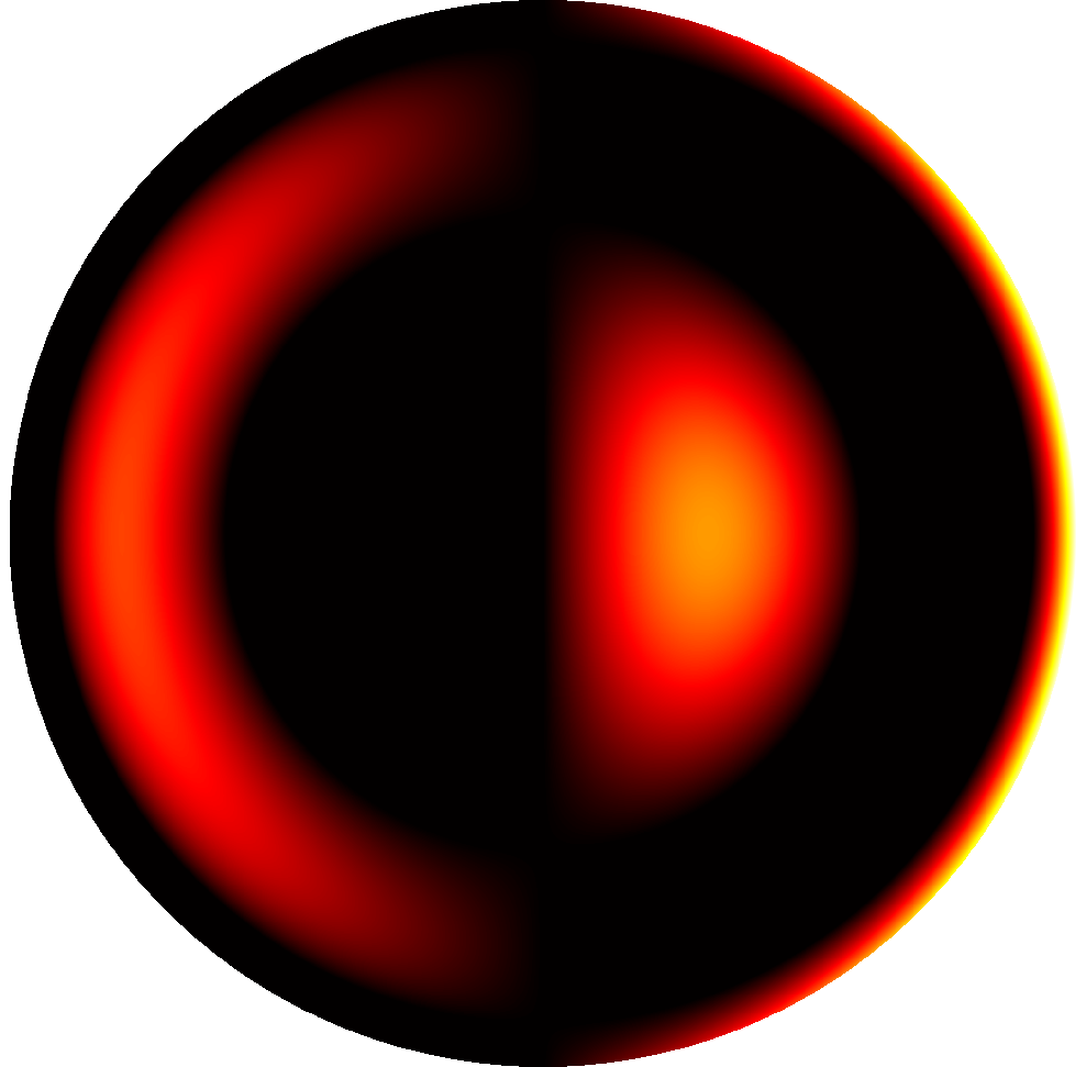
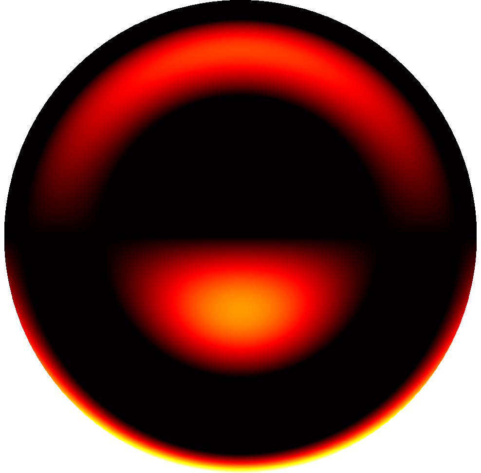
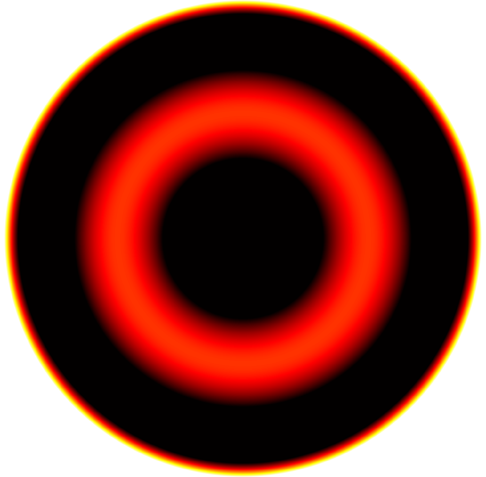
$Z_{13}$	$Z_{14}$	$Z_{15}$

Figure 5: The Zernike polynomials used in the PSF $h_{z}$, with image range $[-1,1]$.

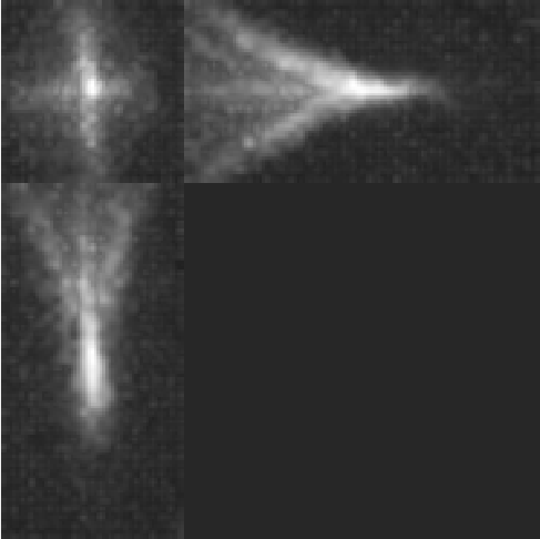
(a) Bead image data (maximum intensity projections)

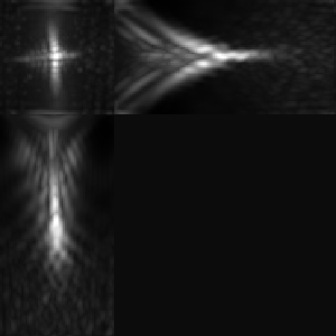
(b) Fitted PSF $h_{z}$, no blur (maximum intensity projections)

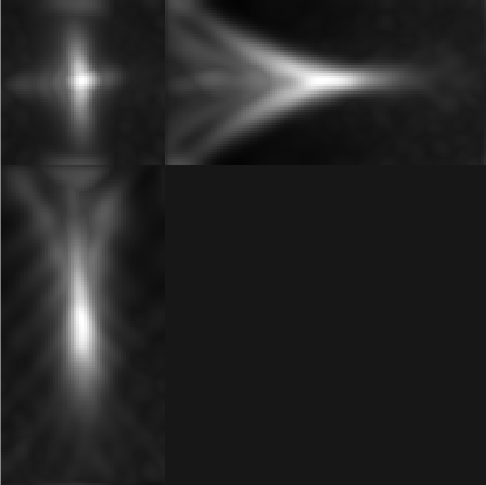
(c) Fitted PSF $h$ with Gaussian blur (maximum intensity projections)

Figure 6: Fitted PSF using Zernike polynomials. In panel (c), we can see the benefits of using the Gaussian blur $g_{\sigma}$ in obtaining an accurate approximation of the bead in (a).

3 Inverse problem

3.1 Problem statement

In this section we formally state the inverse problem of deblurring a light-sheet microscopy image. Let $\Omega\subset\mathbb{R}^{3}$ be a bounded Lipschitz domain and let $L\colon\operatorname{\mathrm{L}}^{p}(\Omega)\to\operatorname{\mathrm{L}}^{2}(\Omega)$ be the forward operator defined by (2.1). Here $1<p<3/2$ is chosen such that the embedding of the $\operatorname{BV}$ space is compact [27]. Clearly, $L$ is linear.

We consider the following inverse problem

$$Lu=\bar{f},$$ (3.1)

where $\bar{f}\in\operatorname{\mathrm{L}}^{2}(\Omega)$ is the exact (noise-free) data. As outlined in Section 2.1, the measurements in light microscopy are corrupted by a combination of Poisson and Gaussian noise. More precisely, the measurement is given by $f=v+w$, where $v\sim Pois(\bar{f})$ is a Poisson distributed random variable with mean $\bar{f}$ and $w$ represents additive zero-mean Gaussian noise. We do not model Gaussian noise statistically and instead, in the spirit of (deterministic) variational regularisation, assume that $w\in\operatorname{\mathrm{L}}^{2}(\Omega)$ is a fixed perturbation with $\mathinner{\!\left\lVert w\right\rVert}_{\operatorname{\mathrm{L}}^{2}(\Omega)}\leqslant\sigma_{G}$ for some known $\sigma_{G}>0$. Poisson noise is typically modelled using the Kullback-Leibler divergence as the data fidelity term [28, 29].

Let us give a brief justification of the inverse problem formulation described in this section [30, 1], from a Bayesian perspective. First, by using the Poisson and Gaussian probability density functions, we have that $p(v|u)=\frac{(Lu)^{v}e^{-(Lu)}}{v!}$ and $p(f|v)=\frac{1}{\sqrt{2\pi}\sigma_{G}}e^{-\frac{1}{2}\left(\frac{f-v}{\sigma_{G}}\right)^{2}}$, and from Bayes’ theorem and conditional probability:

$$p(u,v|f)=\frac{p(f|v)p(v|u)p(u)}{p(f)},$$ (3.2)

where we used that $p(f|u,v)=p(f|v)$. Moreover, we assume that the prior is a Gibbs distribution $p(u)=e^{-\alpha\mathcal{J}(u)}$ for a convex functional $\mathcal{J}(u)$, which we will introduce later. To obtain a maximum a posteriori estimation of $u$ and $v$ (i.e. maximise the posterior distribution $p(u,v|f)$), we take the minimum of the negative log of (3.2) and, after discarding the denominator $p(f)$ and using the Stirling approximation for the factorial $\log v!=v\log v-v$, we obtain the minimisation problem:

$$\operatorname*{arg\,min}_{u,v}\alpha\mathcal{J}(u)+\frac{1}{2\sigma_{G}^{2}}\|f-v\|^{2}+v\log\frac{v}{Lu}+Lu-v,$$ (3.3)

where the first term is the regularisation term and the remaining terms form the data fidelity term.

We will now describe the formal mathematical setting for (3.3) in the context of variational regularisation. This will allow us to show well-posedness of the model, establish convergence rates of the solution with respect to the noise in the measurements and to introduce a discrepancy principle for choosing the value of the regularisation parameter $\alpha$.

First, note that in (3.3), we can perform the minimisation over $v$ only on the data fidelity part of the objective, which can be written as an infimal convolution of the two separate Gaussian and Poisson fidelities. Therefore, we define the following data fidelity term, as proposed in [1]:

$$\Phi(\bar{f},f)\mathrel{\mathop{\mathchar 58\relax}}=\inf_{v\in\operatorname{\mathrm{L}}^{2}_{+}(\Omega)}\left\{\frac{1}{2}\mathinner{\!\left\lVert f-v\right\rVert}^{2}_{\operatorname{\mathrm{L}}^{2}}+D_{KL}(v,\bar{f})\right\},\quad f\in\operatorname{\mathrm{L}}^{2}(\Omega),\,\bar{f}\in\operatorname{\mathrm{L}}^{1}_{+}(\Omega),$$ (3.4)

where $\operatorname{\mathrm{L}}^{1,2}_{+}(\Omega)$ denotes the positive cone in $\operatorname{\mathrm{L}}^{1,2}(\Omega)$ (that is, functions $f\in\operatorname{\mathrm{L}}^{1,2}(\Omega)$ such that $f\geqslant 0$ a.e.) and $D_{KL}$ denotes the Kullback-Leibler divergence which we define as follows

$$D_{KL}(v,\bar{f})\mathrel{\mathop{\mathchar 58\relax}} =\begin{cases}\int_{\Omega}\left(\bar{f}(x)-v(x)+v(x)\log\frac{v(x)}{\bar{f}(x)}\right)\operatorname{d\!}x,\quad&v,\bar{f}\geqslant 0\,\wedge\,\int_{\Omega}v\operatorname{d\!}x=\int_{\Omega}\bar{f}\operatorname{d\!}x=1,\\ +\infty\quad&\text{otherwise,}\end{cases}$$ (3.5)

$$=\begin{cases}\int_{\Omega}v(x)(\log v(x)-\log\bar{f}(x))\operatorname{d\!}x,\qquad\quad\;&v,\bar{f}\geqslant 0\,\wedge\,\int_{\Omega}v\operatorname{d\!}x=\int_{\Omega}\bar{f}\operatorname{d\!}x=1,\\ +\infty\qquad\quad\;&\text{otherwise.}\end{cases}$$

We note that ${\mathinner{\!\left\lvert\int_{\Omega}v(x)\log v(x)\operatorname{d\!}x\right\rvert}<\infty}$ for $v\in\operatorname{\mathrm{L}}^{2}$, since $\operatorname{\mathrm{L}}^{2}$ is continuously embedded into the Orlicz space $\operatorname{\mathrm{L}}\log\operatorname{\mathrm{L}}$ of functions of finite entropy [31, 32]

$$\operatorname{\mathrm{L}}\log\operatorname{\mathrm{L}}(\Omega)\mathrel{\mathop{\mathchar 58\relax}}=\{f\in\operatorname{\mathrm{L}}^{1}(\Omega)\colon\int_{\Omega}\mathinner{\!\left\lvert f(x)\right\rvert}(\log\mathinner{\!\left\lvert f(x)\right\rvert})_{+}\operatorname{d\!}x<\infty\},$$ (3.6)

where $(\cdot)_{+}=\max\{\cdot,0\}$ denotes the positive part.

A proof of the following result can be found in [1], but we provide it here for readers’ convenience.

Proposition 1 (Exactness of the infimal convolution).

For any $\bar{f}\in\operatorname{\mathrm{L}}^{1}_{+}$ such that $\int_{\Omega}\bar{f}\operatorname{d\!}x=1$, there exists a unique solution $v^{*}=v^{*}(\bar{f})$ of (3.4), that is, the infimal convolution is exact. Moreover, the functional $\Phi(\bar{f},\cdot)\colon\operatorname{\mathrm{L}}^{2}\to\mathbb{R}_{+}\cup\{+\infty\}$ is proper, convex and lower semicontinuous.

Proof.

Fix $\bar{f}\in\operatorname{\mathrm{L}}^{1}_{+}$ such that $\int_{\Omega}\bar{f}\operatorname{d\!}x=1$. Then (3.4) is the infimal convolution of the following two functionals on $\operatorname{\mathrm{L}}^{2}$

$$\varphi(g)\mathrel{\mathop{\mathchar 58\relax}}=\chi_{\operatorname{\mathrm{L}}^{2}_{+}}(g)+D_{KL}(g,\bar{f}),\quad\psi(g)\mathrel{\mathop{\mathchar 58\relax}}=\frac{1}{2}\mathinner{\!\left\lVert g\right\rVert}^{2}_{\operatorname{\mathrm{L}}^{2}},\quad g\in\operatorname{\mathrm{L}}^{2}(\Omega),$$

where $\chi$ denotes the characteristic function. The function $\varphi$ is proper, convex, non-negative and lower semicontinuous, while $\psi$ is proper, convex, lower semicontinuous and coercive. Therefore, by [33, Prop. 12.14], the infimal convolution is exact and is itself a proper, convex and lower semicontinuous function. Uniqueness follows from strict convexity of $\psi$. ∎

Now we turn our attention to the lower semicontinuity of the functional $\Phi(\cdot,f)$ in its first argument.

Proposition 2 (Lower semicontinuity).

For any $f\in\operatorname{\mathrm{L}}^{2}_{+}(\Omega)$ such that $\int_{\Omega}f\operatorname{d\!}x=1$ the functional $\Phi(\cdot,f)\colon L^{1}(\Omega)\to\mathbb{R}_{+}\cup\{+\infty\}$ is lower semicontinuous.

Proof.

We have

$$\Phi(g,f) =\inf_{v\in\operatorname{\mathrm{L}}^{2}_{+}(\Omega)}\left\{\frac{1}{2}\mathinner{\!\left\lVert f-v\right\rVert}^{2}_{\operatorname{\mathrm{L}}^{2}}+D_{KL}(v,g)\right\}$$

$$=\frac{1}{2}\mathinner{\!\left\lVert f-v^{*}(g)\right\rVert}^{2}_{\operatorname{\mathrm{L}}^{2}}+D_{KL}(v^{*}(g),g)$$

$$=\frac{1}{2}\mathinner{\!\left\lVert f-v^{*}(g)\right\rVert}^{2}_{\operatorname{\mathrm{L}}^{2}}+\int_{\Omega}v(x)(\log v(x)-\log\bar{f}(x))\operatorname{d\!}x+\chi_{\mathcal{C}}(g),\quad g\in\operatorname{\mathrm{L}}^{1}(\Omega),$$

where $v^{*}(g)$ is as defined in Proposition 1 and $\mathcal{C}\mathrel{\mathop{\mathchar 58\relax}}=\{g\in\operatorname{\mathrm{L}}^{1}_{+}(\Omega)\colon\int_{\Omega}g\operatorname{d\!}x=1\}$. The characteristic function is lower semicontinuous because $\mathcal{C}$ is closed in $\operatorname{\mathrm{L}}^{1}$ and the rest is lower semicontinuous by [1, Thm. 4.1]. ∎

The following fact is easily established.

Proposition 3.

The operator $L\colon\operatorname{\mathrm{L}}^{p}(\Omega)\to\operatorname{\mathrm{L}}^{1}(\Omega)$ defined in (2.1) is continuous for any $p\geqslant 1$. Moreover, if $l$ and $h$ are non-negative and have overlapping support:

$$\operatorname*{supp}(l)\cap\operatorname*{supp}(h)\neq\varnothing,$$

then $\mathbf{1}\notin\mathcal{N}(L)$, where $\mathbf{1}$ is the constant one function and $\mathcal{N}(L)$ is the null space of $L$.

Proof.

By (2.1), we have

$$Lu(x,y,z)=\int_{\Omega}l(s,t,w)h(x-s,y-t,w)u(s,t,w-z)\operatorname{d\!}\mu_{stw},$$

where $\operatorname{d\!}\mu_{stw}\mathrel{\mathop{\mathchar 58\relax}}=\operatorname{d\!}s\operatorname{d\!}t\operatorname{d\!}w$. Noting that the light-sheet PSF $l$ and detection PSF $h$ are bounded from above by some $C_{1},C_{2}>0$, we have that:

$$\|Lu\|_{\operatorname{\mathrm{L}}^{1}} =\int_{\Omega}\left|\int_{\Omega}l(s,t,w)h(x-s,y-t,w)u(s,t,w-z)\operatorname{d\!}\mu_{stw}\right|\operatorname{d\!}\mu_{xyz}$$

$$=\int_{\Omega}\left|\int_{\Omega}l(s,t,w^{\prime}+z)h(x-s,y-t,w^{\prime}+z)u(s,t,w^{\prime})\operatorname{d\!}\mu_{stw^{\prime}}\right|\operatorname{d\!}\mu_{xyz}\quad(\text{by }w^{\prime}=w-z)$$

$$\leqslant C_{1}C_{2}\int_{\Omega}\left|\int_{\Omega}u(s,t,w^{\prime})\operatorname{d\!}\mu_{stw^{\prime}}\right|\operatorname{d\!}\mu_{xyz}$$

$$=C_{1}C_{2}\mathinner{\!\left\lvert\Omega\right\rvert}\left|\int_{\Omega}u(s,t,w^{\prime})\operatorname{d\!}\mu_{stw^{\prime}}\right|$$

$$\leqslant C(p)\mathinner{\!\left\lVert u\right\rVert}_{\operatorname{\mathrm{L}}^{p}},$$

where in the last inequality we applied Hölder’s inequality and $C(p)$ is a constant that depends on $p$ (as well as $C_{1,2}$ and $\Omega$). Hence, we obtain the first claim.

For the second claim, we observe that

$$L\mathbf{1}(x,y,z)=\int_{\Omega}l(s,t,w)h(x-s,y-t,w)\operatorname{d\!}\mu_{stw}\geqslant 0.$$

Consider

$$\int_{\Omega}L\mathbf{1}(x,y,z)\operatorname{d\!}\mu_{xyz} =\int_{\Omega}\int_{\Omega}l(s,t,w)h(x-s,y-t,w)\operatorname{d\!}\mu_{stw}\operatorname{d\!}\mu_{xyz}$$

and let $B_{l,h}\subset\operatorname*{supp}{l}\cap\operatorname*{supp}{h}$. Then, since both $l$ and $h$ are non-negative on $\Omega$, from the last equality above we have that:

$$\int_{\Omega}L\mathbf{1}(x,y,z)\operatorname{d\!}\mu_{xyz} \geqslant\int_{B_{l,h}}l(x,y,z)h(x,y,z)\operatorname{d\!}\mu_{xyz}>0,$$

which proves the second claim. ∎

Remark 1.

Our setting with the measured data $f\in\operatorname{\mathrm{L}}^{2}(\Omega)$ differs slightly from [1], where $f\in\operatorname{\mathrm{L}}^{\infty}(\Omega)$ was assumed.

We will consider the following variational regularisation problem

$$\min_{u\in\operatorname{\mathrm{L}}^{p}_{+}(\Omega)}\Phi(f,Lu)+\alpha\mathcal{J}(u),$$ (3.7)

where $\Phi$ is the infimal-convolution fidelity as defined in (3.4), $\mathcal{J}\colon\operatorname{\mathrm{L}}^{p}\to\mathbb{R}_{+}\cup\{+\infty\}$ is a regularisation functional, $\alpha\in\mathbb{R}_{+}$ is a regularisation parameter and $1<p<3/2$. Without loss of generality, we assume that $\int_{\Omega}\bar{f}\operatorname{d\!}x=1$.

As the regulariser $\mathcal{J}$ we choose the total variation [34]

$$\mathcal{J}(u)=\operatorname{TV}(u)\mathrel{\mathop{\mathchar 58\relax}}=\sup_{\begin{subarray}{c}\xi\in C_{0}^{\infty}(\Omega,\mathbb{R}^{3})\\ \|\xi\|_{\infty}\leqslant 1\end{subarray}}\int_{\Omega}u\operatorname{div}(\xi)\operatorname{d\!}x.$$

By the Rellich–Kondrachov theorem, the space

$$\operatorname{BV}(\Omega)\mathrel{\mathop{\mathchar 58\relax}}=\{u\in\operatorname{\mathrm{L}}^{1}(\Omega)\colon\operatorname{TV}(u)<\infty\},\quad\mathinner{\!\left\lVert u\right\rVert}_{\operatorname{BV}}\mathrel{\mathop{\mathchar 58\relax}}=\mathinner{\!\left\lVert u\right\rVert}_{\operatorname{\mathrm{L}}^{1}}+\operatorname{TV}(u),$$

is compactly embedded into $\operatorname{\mathrm{L}}^{p}(\Omega)$ for $1\leqslant p<3/2$ and continuously embedded into $\operatorname{\mathrm{L}}^{3/2}(\Omega)$ since $\Omega\subset\mathbb{R}^{3}$. Therefore, we consider $\operatorname{TV}\colon\operatorname{\mathrm{L}}^{p}\to\mathbb{R}_{+}\cup\{+\infty\}$

$$\operatorname{TV}(u)\mathrel{\mathop{\mathchar 58\relax}}=\begin{cases}\sup\limits_{\begin{subarray}{c}\xi\in C_{0}^{\infty}(\Omega,\mathbb{R}^{3})\\ \|\xi\|_{\infty}\leqslant 1\end{subarray}}\int_{\Omega}u\operatorname{div}(\xi)\operatorname{d\!}x,\quad&u\in\operatorname{BV}(\Omega),\\ \infty,\quad&u\in\operatorname{\mathrm{L}}^{p}(\Omega)\setminus{\operatorname{BV}(\Omega)}.\end{cases}$$

We will denote by $u^{\dagger}_{\operatorname{TV}}$ the $\operatorname{TV}$-minimising solution of (3.1), i.e. a solution that satisfies

$$Lu^{\dagger}_{\operatorname{TV}}=\bar{f}\text{\quad and \quad$\operatorname{TV}(u^{\dagger}_{\operatorname{TV}})\leqslant\operatorname{TV}(u)$ for all $u$ s.t. $Lu=\bar{f}$.}$$

The existence of such solution is obtained by standard arguments [35]. We will make the reasonable assumption that the $\operatorname{TV}$-minimising solution is positive, i.e. $u^{\dagger}_{\operatorname{TV}}\geqslant 0$ a.e. Due to the positivity of the kernels involved in (2.1), it is clear that $u^{\dagger}_{\operatorname{TV}}\geqslant 0$ implies $Lu^{\dagger}_{\operatorname{TV}}=\bar{f}\geqslant 0$.

Since by Proposition 1 the infimal convolution (3.4) is exact, we can equivalently rewrite (3.7) as follows

$$\min_{\begin{subarray}{c}u\in\operatorname{\mathrm{L}}^{p}_{+}(\Omega)\\ v\in\operatorname{\mathrm{L}}^{2}_{+}(\Omega)\end{subarray}}\frac{1}{2}\mathinner{\!\left\lVert f-v\right\rVert}^{2}_{\operatorname{\mathrm{L}}^{2}}+D_{KL}(v,Lu)+\alpha\mathcal{J}(u).$$ (3.8)

Existence of minimisers in (3.7) and (3.8) is obtained by standard arguments [1, Thm. 4.1].

Proposition 4.

Each of the opimisation problems (3.7) and (3.8) admits a unique minimiser.

We will also need the following coercivity result.

Proposition 5.

The functional $\Phi(f,\cdot)\colon\operatorname{\mathrm{L}}^{1}(\Omega)\to\mathbb{R}_{+}\cup\{+\infty\}$ is strongly coercive with exponent $2$, i.e. there exists a constant $C>0$ such that

$$\Phi(f,g)\geqslant C\mathinner{\!\left\lVert g-f\right\rVert}_{\operatorname{\mathrm{L}}^{1}}^{2},\quad g\in\operatorname{\mathrm{L}}^{1}(\Omega).$$

Proof.

Using Pinsker’s inequality for the Kullback-Leibler divergence, we get

$$\Phi(f,g) =\inf_{v\in\operatorname{\mathrm{L}}^{2}_{+}}\frac{1}{2}\mathinner{\!\left\lVert v-f\right\rVert}_{\operatorname{\mathrm{L}}^{2}}^{2}+D_{KL}(v,g)$$

$$\geqslant\inf_{v\in\operatorname{\mathrm{L}}^{2}_{+}}\frac{1}{2}\mathinner{\!\left\lVert v-f\right\rVert}_{\operatorname{\mathrm{L}}^{2}}^{2}+\mathinner{\!\left\lVert g-v\right\rVert}_{\operatorname{\mathrm{L}}^{1}}^{2}$$

$$\geqslant 2C\inf_{v\in\operatorname{\mathrm{L}}^{2}_{+}}\mathinner{\!\left\lVert v-f\right\rVert}_{\operatorname{\mathrm{L}}^{1}}^{2}+\mathinner{\!\left\lVert g-v\right\rVert}_{\operatorname{\mathrm{L}}^{1}}^{2}$$

for some $C>0$. Note that Pinsker’s inequality assumes that $f,g\geqslant 0$ and $\inf_{\Omega}f\operatorname{d\!}x=\int_{\Omega}g\operatorname{d\!}x=1$, which we ensure by definition in (3.5).

Now, using the inequality $\frac{1}{2}(a+b)^{2}\leqslant a^{2}+b^{2}$ that holds for all $a,b\in\mathbb{R}$ and the triangle inequality, we obtain the claim

$$\Phi(f,g) \geqslant C\inf_{v\in\operatorname{\mathrm{L}}^{2}_{+}}\left(\mathinner{\!\left\lVert v-f\right\rVert}_{\operatorname{\mathrm{L}}^{1}}+\mathinner{\!\left\lVert g-v\right\rVert}_{\operatorname{\mathrm{L}}^{1}}\right)^{2}$$

$$\geqslant C\inf_{v\in\operatorname{\mathrm{L}}^{2}_{+}}\mathinner{\!\left\lVert v-f+g-v\right\rVert}_{\operatorname{\mathrm{L}}^{1}}^{2}$$

$$=C\mathinner{\!\left\lVert g-f\right\rVert}_{\operatorname{\mathrm{L}}^{1}}^{2}.$$

∎

3.2 Convergence rates

Our aim in this section is to establish convergence rates of minimisers of (3.7) as the amount of noise in the data decreases. But first we need to specify what we mean by the amount of noise in our setting.

We argue as follows. Since the noise in the measurement is generated sequentially, i.e. photo-electrons are first counted by the sensor leading to a Poisson noise and later they are collected by the electronic circuit generating an additive Gaussian noise, for any exact data $\bar{f}$ there exists $\bar{z}\sim Pois(\bar{f})$ such that $D_{KL}(\bar{z},\bar{f})\leqslant\gamma$, where $\gamma>0$ depends on the exposure time $t$ and vanishes as $t\to\infty$ [28]. Further, there exists $w\in\operatorname{\mathrm{L}}^{2}(\Omega)$ with $\mathinner{\!\left\lVert w\right\rVert}_{\operatorname{\mathrm{L}}^{2}}\leqslant\sigma_{G}$ such that $f=\bar{z}+w$. Since $\bar{z}\geqslant 0$ is feasible in (3.4), we get the following upper bound on the fidelity term (3.4) evaluated at the measurement $f$ and the exact data $\bar{f}$

$$\Phi(\bar{f},f)\leqslant\frac{1}{2}\mathinner{\!\left\lVert f-\bar{z}\right\rVert}^{2}_{\operatorname{\mathrm{L}}^{2}}+D_{KL}(\bar{z},\bar{f})=\frac{1}{2}\mathinner{\!\left\lVert w\right\rVert}^{2}_{\operatorname{\mathrm{L}}^{2}}+D_{KL}(\bar{z},\bar{f})\leqslant\frac{\sigma_{G}^{2}}{2}+\gamma.$$ (3.9)

The standard tool for establishing convergence rates are Bregman distances associated with the regulariser $\mathcal{J}$. We briefly recall the necessary definitions.

Definition 6.

Let $X$ be a Banach space and $\mathcal{J}\colon X\to\mathbb{R}_{+}\cup\{+\infty\}$ a proper convex functional. The generalised Bregman distance between $x,y\in X$ corresponding to the subgradient $q\in\partial\mathcal{J}(y)$ is defined as follows

$$D_{\mathcal{J}}^{q}(x,y)\mathrel{\mathop{\mathchar 58\relax}}=\mathcal{J}(x)-\mathcal{J}(y)-\langle q,x-y\rangle.$$

Here $\partial\mathcal{J}(v)$ denotes the subdifferential of $\mathcal{J}$ at $y\in X$. If, in addition, $p\in\partial\mathcal{J}(x)$, the symmetric Bregman distance between $x,y\in X$ corresponding to the subgradients $p,q$ is defined as follows

$$D_{\mathcal{J}}^{p,q}(x,y)\mathrel{\mathop{\mathchar 58\relax}}=D_{\mathcal{J}}^{q}(x,y)+D_{\mathcal{J}}^{p}(y,x)=\langle p-q,x-y\rangle.$$

To obtain convergence rates, an additional assumption on the regularity of the $\operatorname{TV}$-minimising solution, called the source condition, needs to be made. We use the following variant [36].

Assumption 7 (Source condition).

There exists an element $\mu^{\dagger}\in L^{\infty}(\Omega)$ such that

$$q^{\dagger}\mathrel{\mathop{\mathchar 58\relax}}=L^{*}\mu^{\dagger}\in\partial\mathcal{J}(u^{\dagger}_{\operatorname{TV}}).$$

3.2.1 Parameter choice rules

Let us summarise what we know about the fidelity function $\Phi$ as defined in (3.4), the regularisation functional $\operatorname{TV}$ and the forward operator $L$:

• $\Phi(f,\cdot)$ is proper, convex and coercive (Proposition 5) in $\operatorname{\mathrm{L}}^{1}(\Omega)$;

• $\Phi(\cdot,\cdot)$ is jointly convex [37] and lower semicontinuous (Propositions 1 and 2);

• $\Phi(f,g)=0$ if and only if $f=g$;

• $\operatorname{TV}\colon\operatorname{\mathrm{L}}^{1}(\Omega)\to\mathbb{R}\cup\{+\infty\}$ is proper, convex and lower semicontinuous [27] and its null space is given by $\mathcal{N}(\operatorname{TV})=\operatorname{span}\{\mathbf{1}\}$, where $\mathbf{1}$ denotes the constant one function;

• $\operatorname{TV}$ is coercive on the complement of its null space in $\operatorname{\mathrm{L}}^{1}(\Omega)$ [27];

• $L\colon\operatorname{\mathrm{L}}^{p}(\Omega)\to\operatorname{\mathrm{L}}^{1}(\Omega)$ is continuous and $\mathcal{N}(\operatorname{TV})\cap\mathcal{N}(L)=\{0\}$ (Proposition 3).

Using these facts and slightly modifying the proofs from [38], we obtain the following

Theorem 8 (Convergence rates under a priori parameter choice rules).

Let assumptions made in Section 3.1 hold and let the source condition (7) be satisfied at the $\operatorname{TV}$-minimising solution $u^{\dagger}_{\operatorname{TV}}$. Let $u_{\sigma_{G},\gamma}$ be a solution of (3.7) and let $\alpha$ be chosen such that

$$\alpha(\sigma_{G},\gamma)=O(\sigma_{G}+\sqrt{\gamma}).$$

Then

$$D^{q^{\dagger}}_{\operatorname{TV}}(u_{\sigma_{G},\gamma},u^{\dagger}_{\operatorname{TV}})=O(\sigma_{G}+\sqrt{\gamma}),$$

where $q^{\dagger}=L^{*}\mu^{\dagger}$ is the subgradient from 7 and $\sigma_{G},\gamma>0$ are as defined in (3.9).

Proof.

The proof is similar to [38, Thm. 3.9]. ∎

In a similar manner, we can obtain convergence rates for an a posteriori parameter choice rule known as the discrepancy principle [39, 40, 41]. Let $f$ be the noisy data and $\delta>0$ the amount of noise such that $\Phi(\bar{f},f)\leqslant\delta$, where $\Phi$ is as defined in (3.4). In our case, $\delta=\frac{\sigma_{G}^{2}}{2}+\gamma$ by (3.9). The discrepancy principle amounts to selecting $\alpha=\alpha(f,\delta)$ such that

$$\alpha=\sup\{\alpha>0\colon\Phi(Lu^{\alpha},f)\leqslant\tau\delta\},$$ (3.10)

where $u^{\alpha}$ is the regularised solution corresponding the the regularisation parameter $\alpha$ and $\tau>1$ is a parameter.

Again, slightly modifying the proofs from [38], we obtain the following

Theorem 9 (Convergence rates under the discrepancy principle).

Let assumptions made in Section 3.1 hold and let the source condition (7) be satisfied at the $\operatorname{TV}$-minimising solution $u^{\dagger}_{\operatorname{TV}}$. Let $u_{\sigma_{G},\gamma}$ be a solution of (3.7) with $\alpha$ chosen according to the discrepancy principle (3.10). Then

$$D^{q^{\dagger}}_{\operatorname{TV}}(u_{\sigma_{G},\gamma},u^{\dagger}_{\operatorname{TV}})=O(\sigma_{G}+\sqrt{\gamma}),$$

where $q^{\dagger}=L^{*}\mu^{\dagger}$ is the subgradient from 7 and $\sigma_{G},\gamma>0$ are as defined in (3.9).

Proof.

The proof is similar to [38, Thm. 4.10]. ∎

4 Solving the minimisation problem

4.1 PDHG for infimal convolution model

In practice, due to the joint convexity of the Kullback-Leibler divergence, we solve the minimisation problem (3.8), where we treat the reconstructed sample $u$ and the Gaussian denoised image $v$ jointly and, in addition, we impose lower and upper bound constraints on $u$ and $v$ by including the corresponding characteristic functions in the objective:

$$\min_{u,v}\left\{\alpha\operatorname{TV}(u)+\frac{1}{2\sigma_{G}^{2}}\|f-v\|_{2}^{2}+D_{KL}(v,Lu)+\chi_{[l_{1},l_{2}]^{2N}}([u,v]^{T})\right\}.$$ (4.1)

Note that the objective function in (4.1) is a sum of convex functions (the Kullback-Leibler divergence $D_{KL}$ is jointly convex [42]), and therefore is itself convex. We then write the problem (4.1) as:

$$\min_{w}\left\{G(w)+\sum_{i=1}^{m}H_{i}(L_{i}w)\right\},$$ (4.2)

where we solve for $w=\begin{bmatrix}u\\ v\end{bmatrix}$, $m=3$ and:

$$G(w)=\chi_{[l_{1},l_{2}]^{2N}}\left(\begin{bmatrix}u\\ v\end{bmatrix}\right),$$ (4.3)

$$H_{1}(\cdot)=\frac{1}{2\sigma_{G}^{2}}\left\|\cdot-f\right\|_{2}, L_{1}=\begin{bmatrix}0&1\end{bmatrix},$$ (4.4)

$$H_{2}(w)=D_{KL}(v,u), L_{2}=\begin{bmatrix}L&0\\ 0&1\end{bmatrix},$$ (4.5)

$$H_{3}(\cdot)=\alpha\left\|\cdot\right\|_{1}, L_{3}=\begin{bmatrix}\nabla_{x}&0\\ \nabla_{y}&0\\ \nabla_{z}&0\end{bmatrix},$$ (4.6)

where $L$ is the forward operator corresponding to the image formation model from Section 2.1.

Rather than solving the problem (4.2) directly, a common approach is to reformulate it as a saddle point problem using the Fenchel conjugate $G^{*}(y)=\sup_{z}\langle z,y\rangle-G(z)$. For proper, convex and lower semicontinuous function $G$, we have that $G^{**}=G$, so (4.2) can be written as the saddle point problem

$$\min_{w}\sup_{y_{1},\ldots,y_{m}}\left\{G(w)+\sum_{i=1}^{m}\langle y_{i},L_{i}x\rangle-H_{i}^{*}(y_{i})\right\},$$ (4.7)

and by swapping the $\min$ and the $\sup$ and applying the definition of the convex conjugate $G^{*}$, one obtains the dual of (4.2):

$$\max_{y_{1},\ldots,y_{m}}\left\{-G^{*}(-\sum_{i=1}^{m}L_{i}^{*}y_{i})-\sum_{i=1}^{m}H_{i}^{*}(y_{i})\right\}.$$ (4.8)

The saddle point problem (4.7) is commonly solved using the primal-dual hybrid gradient (PDHG) algorithm [43, 44, 6], and by doing so, both the primal problem (4.2) and the dual (4.8) are solved. We apply the variant of PDHG from [45], which accounts for the sum of composite terms terms $H_{i}\circ L_{i}$. Given an initial guess for $(w_{0},y_{1,0},\ldots,y_{m,0})$ and the parameters $\sigma,\tau>0$, and $\rho\in[\epsilon,2-\epsilon]$ for some $\epsilon>0$, each iteration $k\geqslant 0$ consists of the following steps:

$$1.\quad\tilde{w}_{k+1}\mathrel{\mathop{\mathchar 58\relax}}=\operatorname{prox}_{\tau G}(w_{k}-\tau\sum_{i=1}^{m}L_{i}^{*}y_{i,k}),$$

$$2.\quad w_{k+1}\mathrel{\mathop{\mathchar 58\relax}}=\rho_{k}\tilde{w}_{k+1}+(1-\rho_{k})w_{k},$$

$$3.\quad\forall i=1,\ldots,m\mathrel{\mathop{\mathchar 58\relax}}\quad\tilde{y}_{i,k+1}\mathrel{\mathop{\mathchar 58\relax}}=\operatorname{prox}_{\sigma H_{i}^{*}}\left(y_{i,k}+\sigma L_{i}(2\tilde{w}_{k+1}-w_{k})\right),$$

$$4.\quad\forall i=1,\ldots,m\mathrel{\mathop{\mathchar 58\relax}}\quad y_{i,k+1}\mathrel{\mathop{\mathchar 58\relax}}=\rho\tilde{y}_{i,k+1}+(1-\rho)y_{i,k}.$$ (4.9)

where for a proper, lower semi-continuous, convex function $G$, $\operatorname{prox}_{\tau G}$ is its proximal operator, defined as:

$$\operatorname{prox}_{\tau G}(y)\mathrel{\mathop{\mathchar 58\relax}}=\operatorname*{arg\,min}_{x}\left\{\frac{1}{2\tau}\|x-y\|_{2}^{2}+G(x)\right\}.$$ (4.10)

The iterates $(w_{k})_{k\in\mathbb{N}}$ and $(y_{i,k})_{k\in\mathbb{N}}$ ($i=1,\ldots,m$) are shown to converge if the parameters $\sigma$ and $\tau$ are chosen such that $\sigma\tau\|\sum_{i=1}^{m}L_{i}^{*}L_{i}\|\leqslant 1$ (see [45], Theorem 5.3). In step 3 in (4.9), we use Moreau’s identity to obtain $\operatorname{prox}_{\sigma H^{*}_{i}}$ from $\operatorname{prox}_{H_{i}/\sigma}$:

$$\operatorname{prox}_{\sigma H_{i}^{*}}(y)+\sigma\operatorname{prox}_{H_{i}/{\sigma}}(y/{\sigma})=y.$$ (4.11)

As a stopping criterion, one can use the primal-dual gap i.e. the difference between the primal objective cost at the current iterate and the dual objective cost at the current (dual) iterate:

$$D_{pd}(w,y_{1},\ldots,y_{m})=G(w)+\sum_{i=1}^{m}H_{i}(L_{i}w)+G^{*}(-\sum_{i=1}^{m}L_{i}^{*}y_{i})+\sum_{i=1}^{m}H_{i}^{*}(y_{i})$$ (4.12)

Due to strong duality, optimality is reached when the primal-dual gap is zero, so a practical stopping criterion is when the gap reaches a certain threshold set in advance.

Lastly, note that the optimisation is performed jointly over both $u$ and $v$, which introduces a difficulty for the term $H_{2}(L_{2}w)$ in Step 3 above, as this requires the proximal operator of the joint Kullback-Leibler divergence $D_{KL}(u,v)$. Similarly, the computation of the primal-dual gap in (4.12) requires the convex conjugate of the joint Kullback-Leibler divergence. We describe the details of these computations in Section 4.2 and Section 4.3 respectively.

4.2 Computing the proximal operator of the joint Kullback–Leibler divergence

When writing the optimisation problem in the form (4.2), it is common that the functions $G$ and $H_{i}$ ($i=1,\ldots,m$) are “simple”, meaning that their proximity operators have a closed form solution or can be easily computed with high precision. This is certainly true for $G$ and $H_{1}$, but not obvious for the joint Kullback-Leibler divergence.

First, for discrete images $u=[u_{1},\ldots,u_{N}]^{T},[v_{1},\ldots,v_{N}]^{T}$, the definition (3.5) becomes:

$$D_{KL}(v,u)=\sum_{j=1}^{N}u_{j}-v_{j}+v_{j}\log\frac{v_{j}}{u_{j}}$$ (4.13)

and then:

$$\operatorname{prox}_{\gamma D_{KL}}(u^{*},v^{*}) =\operatorname*{arg\,min}_{u,v}\left\{D_{KL}(u,v)+\frac{1}{2\gamma}\left\|\begin{bmatrix}u\\ v\end{bmatrix}-\begin{bmatrix}u^{*}\\ v^{*}\end{bmatrix}\right\|^{2}_{2}\right\}$$

$$=\operatorname*{arg\,min}_{u,v}\left\{\sum_{j=1}^{N}u_{j}-v_{j}+v_{j}\log\frac{v_{j}}{u_{j}}+\frac{1}{2\gamma}[(u_{j}-u_{j}^{*})^{2}+(v_{j}-v_{j}^{*})^{2}]\right\}$$

$$=\sum_{j=1}^{N}\operatorname*{arg\,min}_{u_{j},v_{j}}\Phi(u_{j},v_{j}),$$ (4.14)

where we define the function $\Phi$ as:

$$\Phi(u_{j},v_{j})\mathrel{\mathop{\mathchar 58\relax}}=u_{j}-v_{j}+v_{j}\log\frac{v_{j}}{u_{j}}+\frac{1}{2\gamma}[(u_{j}-u_{j}^{*})^{2}+(v_{j}-v_{j}^{*})^{2}].$$ (4.15)

To find the minimiser of $\Phi(u_{j},v_{j})$, we let its gradient be equal to zero:

$$\begin{cases}\partial_{u_{j}}\Phi(u_{j},v_{j})=0\\ \partial_{v_{j}}\Phi(u_{j},v_{j})=0\end{cases}\iff\begin{cases}1-\frac{v_{j}}{u_{j}}+\frac{1}{\gamma}(u_{j}-u_{j}^{*})=0\\ \log v_{j}-\log u_{j}+\frac{1}{\gamma}(v_{j}-v_{j}^{*})=0\end{cases}$$ (4.16)

In the second equation, we write $u_{j}$ as a function of $v_{j}$, which we substitute in the first equation to obtain:

$$\begin{cases}1-e^{-\frac{1}{\gamma}(v_{j}-v_{j}^{*})}+\frac{1}{\gamma}\left(v_{j}e^{\frac{1}{\gamma}(v_{j}-v_{j}^{*})}-u_{j}^{*}\right)=0\\ u_{j}=v_{j}e^{\frac{1}{\gamma}(v_{j}-v_{j}^{*})}\end{cases}$$ (4.17)

The first equation is then solved using Newton’s method, where the iteration is given by:

$$v_{j}^{(k+1)}=v_{j}^{(k)}-\frac{\gamma-\gamma e^{-\frac{1}{\gamma}(v_{j}^{(k)}-v_{j}^{*})}+v_{j}^{(k)}e^{\frac{1}{\gamma}(v_{j}^{(k)}-v_{j}^{*})}-u_{j}^{*}}{e^{-\frac{1}{\gamma}(v_{j}^{(k)}-v_{j}^{*})}+(1+\frac{1}{\gamma}v_{j}^{(k)})e^{\frac{1}{\gamma}(v_{j}^{(k)}-v_{j}^{*})}}.$$ (4.18)

4.3 Computing the convex conjugate of the joint Kullback–Leibler divergence

We compute the convex conjugate of the discrete joint Kullback-Leibler divergence $D_{KL}(v,u)$ in (4.13) for $u,v\in[l_{1},l_{2}]^{N}$:

$$D^{*}_{KL}(v^{*},u^{*}) =\sup_{v,u\in[l_{1},l_{2}]^{N}}\left\{\left\langle\begin{bmatrix}u\\ v\end{bmatrix},\begin{bmatrix}u^{*}\\ v^{*}\end{bmatrix}\right\rangle-D_{KL}(v,u)\right\}$$

$$=\sup_{v,u\in[l_{1},l_{2}]^{N}}\left\{\sum_{j=1}^{N}u_{j}u_{j}^{*}+v_{j}v_{j}^{*}-u_{j}+v_{j}-v_{j}\log\frac{v_{j}}{u_{j}}\right\}$$

$$=\sum_{j=1}^{N}\sup_{v_{j},u_{j}\in[l_{1},l_{2}]}\Psi(v_{j},u_{j}),$$ (4.19)

where $\Psi$ is defined as:

$$\Psi(v_{j},u_{j})\mathrel{\mathop{\mathchar 58\relax}}=u_{j}u_{j}^{*}+v_{j}v_{j}^{*}-u_{j}+v_{j}-v_{j}\log\frac{v_{j}}{u_{j}}.$$ (4.20)

To solve the optimisation problem on the last line in (4.19), we write the KKT conditions (where we use $u,v$ instead of $u_{j},v_{j}$ to simplify the notation:

$$-\nabla\Psi(v,u) +\sum_{i=1}^{4}\mu_{i}\nabla g_{i}(v,u)=0,$$ (4.21)

$$g_{i}(v,u) \leqslant 0,\quad\forall i=1,\ldots,4,$$ (4.22)

$$\mu_{i} \geqslant 0,\quad\forall i=1,\ldots,4,$$ (4.23)

$$\mu_{i}g_{i}(v,u) =0,\quad\forall i=1,\ldots,4.$$ (4.24)

where the functions $g_{i}$ correspond to the bound constraints:

$$g_{1}(v,u) =u-l_{2};$$ (4.25)

$$g_{2}(v,u) =v-l_{2};$$ (4.26)

$$g_{3}(v,u) =-u+l_{1};$$ (4.27)

$$g_{4}(v,u) =-v+l_{1};$$ (4.28)

Noting that (4.21) is equivalent to:

$$-u^{*}+1-\frac{v}{u}+\mu_{1}-\mu_{3}=0,$$ (4.30)

$$-v^{*}+\log v-\log u+\mu_{2}-\mu_{4}=0,$$ (4.31)

we solve the last two equations by using the complementarity conditions (4.24) for cases when the Lagrange multipliers $\mu_{i}$ are zero or non-zero.

5 Numerical results

In this section, we describe a number of numerical experiments that illustrate the performance of our deconvolution method. We start with four examples of simulated data, where we are able to quantify the reconstructed image in relation to the known ground truth image. Then, we show how our method performs on microscopy data, where we reconstruct an image of spherical beads and a sample of a Marchantia thallus.

5.1 Simulated data

We consider four images of size $128\times 125\times 64$: a $5\times 5\times 5$ grid of beads where the effect of the light-sheet in the $z$ coordinate and the shape of the objective PSF are noticeable, a piecewise constant image of “steps” where the Poisson noise affects each step differently based on intensity, and an image that replicates a realistic biological samples of tissue. These are shown in the top row of Figure 7.

To obtain the measured data, we proceed as follows. Given the ground truth image $u_{0}$, the forward operator described in Section 2.1 is applied to obtain the blurred image $Lu_{0}$. The parameters for the forward model are taken to be those of the microscope used in the experimental setup, and are given in Table 2. Then, the image corrupted with a mixture of Poisson and Gaussian noise. For the vectorised image $Lu_{0}$, at each pixel $i=1,\ldots,N$, the Poisson noise component follows the Poisson distribution with parameter $(Lu_{0})_{i}$ and the additive Gaussian component has zero mean and standard deviation $\sigma_{G}=10$. The original image, which has intensity in $[0,1]$ is scaled so that the intensity of $Lu_{0}$ is in $[0,2000]$, to replicate a realistic scenario for the Poisson noise intensity. The resulting simulated measured data is shown in the bottom row of Figure 7.

Parameter	Value	Description, units
$n$	$1.35$	refractive index
$NA_{h}$	$1$	numerical aperture (objective lens)
$NA_{l}$	$0.25$	numerical aperture (light-sheet)
$\lambda_{h}$	$0.525$	wave length (objective lens), $\mu m$
$\lambda_{l}$	$0.488$	wave length (light-sheet), $\mu m$
$px_{x}$	$0.3250$	pixel size ($x$), $\mu m$
$px_{y}$	$0.3250$	pixel size ($y$), $\mu m$
$step_{z}$	$1$	light-sheet step size ($z$), $\mu m$

Table 2: Forward model parameters used in Section 5.

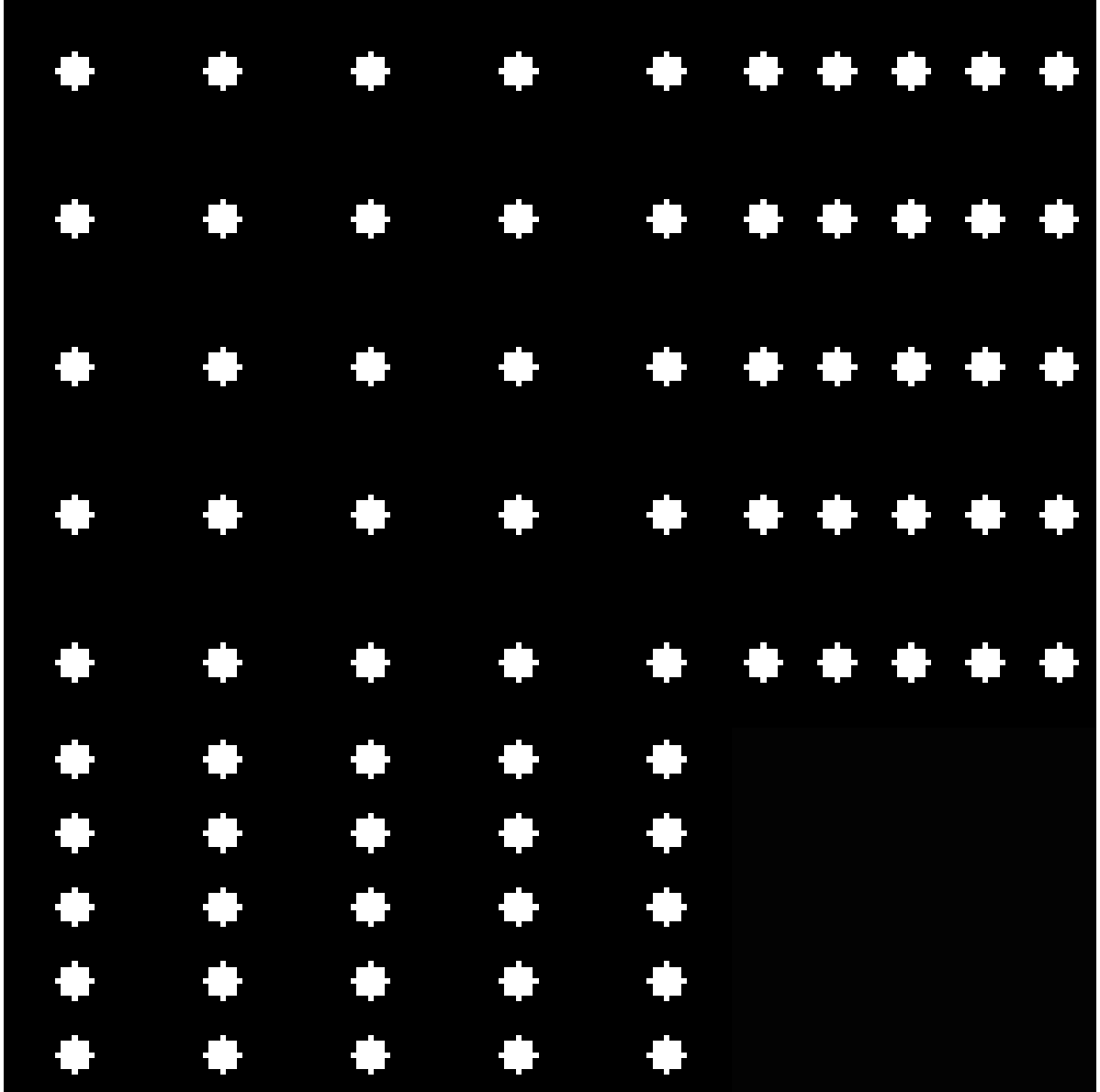
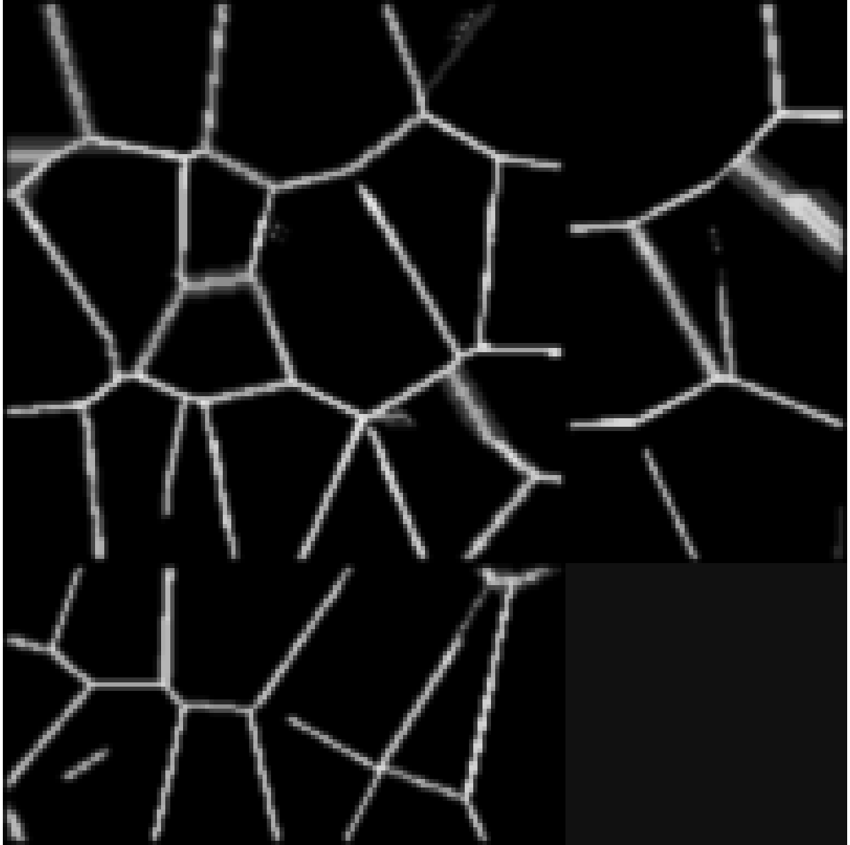
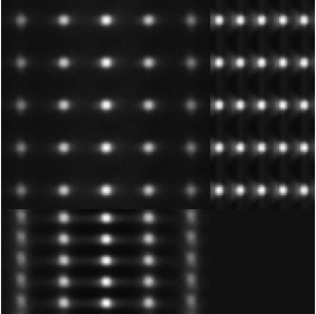
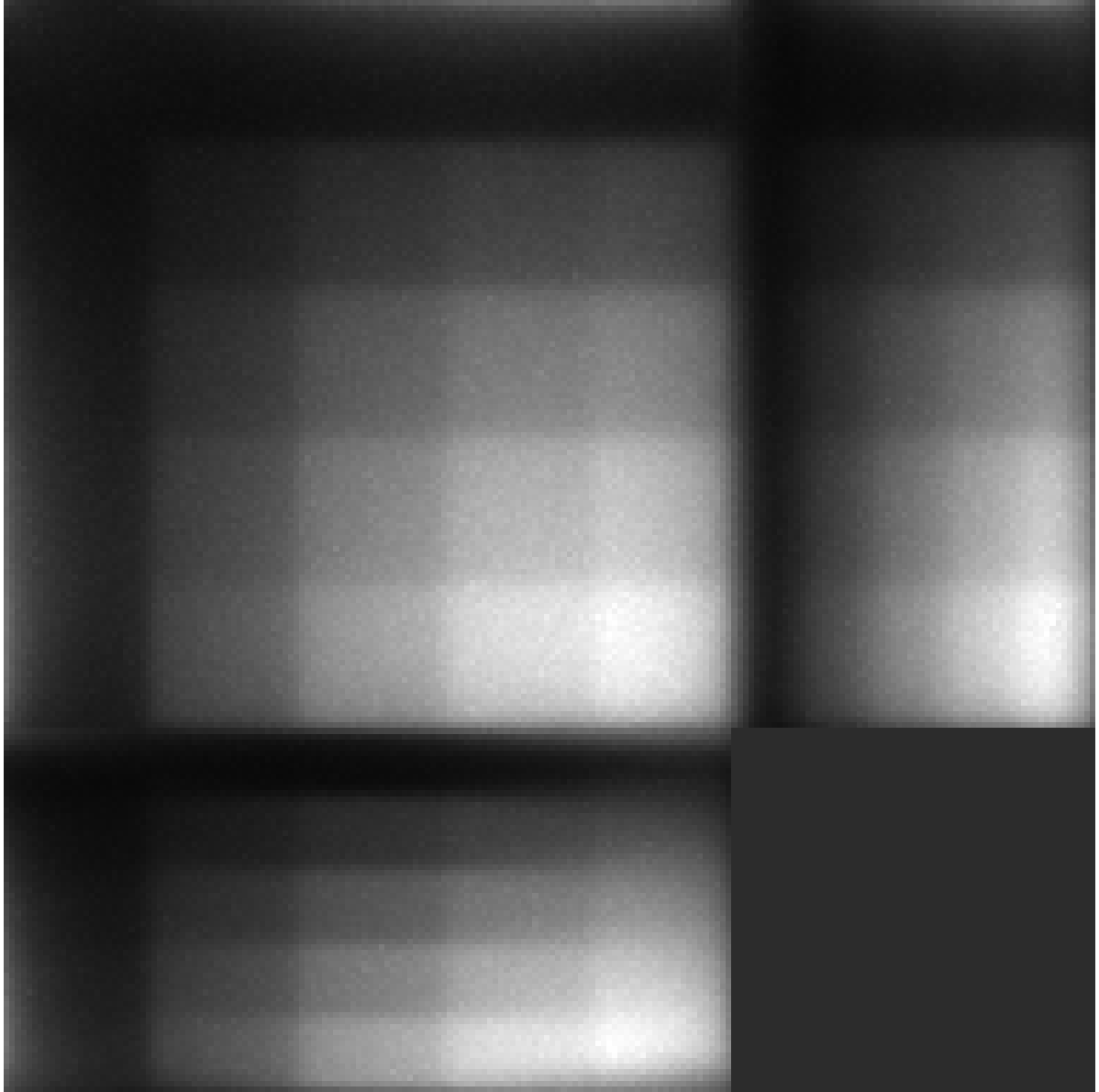
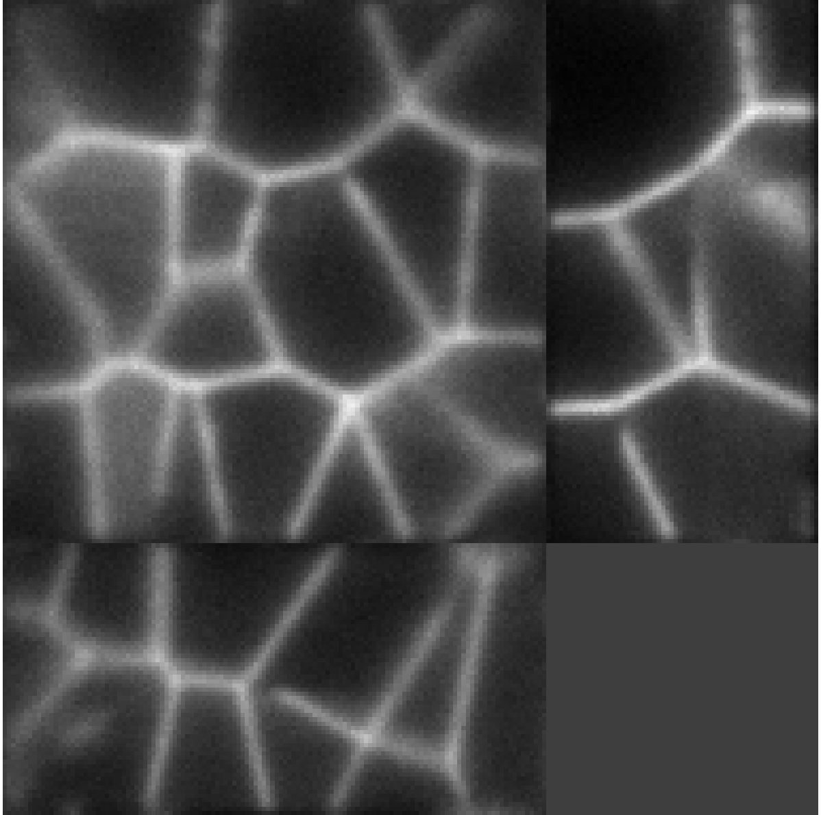
Figure 7: Ground truth (top row) and measured images (bottom row), shown using maximum intensity projections, except for tissue, where slices in each direction are shown.

We compare the reconstruction obtained using the proposed approach, which we will refer to as LS-IC (light-sheet - infimal convolution), with the reconstructions obtained by using an $L^{2}$ data fidelity term instead of the infimal convolution term, or using a convolution operator corresponding to the objective PSF instead of the light-sheet forward model from Section 2.1. Specifically, we compare the solution of (4.1) with the solutions to the following problems, all solved using PDHG as described in Section 4:

$$\min_{u}\left\{\alpha\operatorname{TV}(u)+\frac{1}{2\sigma_{G}^{2}}\|f-Hu\|_{2}^{2}+\chi_{[0,B]^{2N}}([u,v]^{T})\right\},$$ (PSF-L2)

$$\min_{u,v}\left\{\alpha\operatorname{TV}(u)+\frac{1}{2\sigma_{G}^{2}}\|f-v\|_{2}^{2}+D_{KL}(v,Hu)+\chi_{[0,B]^{2N}}([u,v]^{T})\right\},$$ (PSF-IC)

$$\min_{u}\left\{\alpha\operatorname{TV}(u)+\frac{1}{2\sigma_{G}^{2}}\|f-Lu\|_{2}^{2}+\chi_{[0,B]^{2N}}([u,v]^{T})\right\},$$ (LS-L2)

where $H$ is the convolution operator with the detection objective PSF $h_{z}$ as given in (2.15).

For each test image and each method above, the PDHG parameters $\rho$ and $\sigma$ used are given in Table 3 and $\tau$ is set to $\tau=1/\sigma\|\sum_{i=1}^{m}L_{i}^{*}L_{i}\|$ to ensure convergence according to Theorem 5.3 in [45]. As a stopping criterion, we used the primal-dual gap (4.12), normalised by the number of pixels $N$ and the dynamic range of the measured image $f$:

$$\tilde{D}_{pd}=\frac{D_{pd}}{N\cdot\max_{j=1,\ldots,N}f_{j}},$$ (5.1)

with a threshold of $10^{-6}$ and a maximum number of $10000$ iterations.

method		LS-IC			LS-L2			PSF-IC			PSF-L2
image	beads	steps	tissue	beads	steps	tissue	beads	steps	tissue	beads	steps	tissue
$\rho$	0.9	0.9	0.9	0.9	0.9	0.9	0.9	0.9	0.8	0.9	0.9	0.9
$\sigma$	0.0001	0.0001	0.00001	0.0001	0.001	0.0001	0.0001	0.0001	0.0001	0.0001	0.001	0.0001

Table 3: Values of the PDHG parameters $\rho$ and $\sigma$ used in the numerical experiments with simulated data.

The results of the four methods applied to the test images are given in Figure 8 and quantitative results are given in Table 4. For each test image and each method, the regularisation parameter has been chosen to optimise the normalised $l^{2}$ error and the structural similarity index (SSIM) respectively.

We note that PSF-L2 and PSF-IC perform particularly poorly, highlighting the importance of an accurate representation of the image formation model instead of simply using the detection objective PSF as the forward operator. Comparing LS-IC and LS-L2, we see better results when using the infimal convolution data fidelity for the beads and the steps image, both visually and quantitatively. The deblurring is performed better on the beads image, while on the steps image we see a better denoising effect, especially along the edges in the image. For the tissue image, both fidelities give comparable results, but as we see in Figure 9, when the ground truth is not known, choosing $\alpha$ using the discrepancy principle gives a better result for the infimal convolution model.

The reconstructions shown in Figure 9 are obtained by applying the discrepancy principle corresponding to each method. For LS-IC, we choose a value of $\alpha$ such that it satisfies a variation of the discrepancy principle given in (3.10), where we enforce that the single noise fidelities are bounded by their respective noise bounds, rather than the sum of the fidelities being bounded by the sum of the noise bounds, as stated in (3.10). While both versions give good results, we found the former to give more accurate reconstructions. Here, the bound on the Poisson noise is set to $\frac{1}{2}$, motivated by the following lemma from [46], which gives the expected value of the Kullback-Leibler divergence:

Lemma 10.

Let $Y_{\beta}$ be a Poisson random variable with expected value $\beta$ and consider the function:

$$F(Y_{\beta})=2\left\{Y_{\beta}\log\left(\frac{Y_{\beta}}{\beta}\right)+\beta-Y_{\beta}\right\}.$$

Then, for large $\beta$,the following estimate of the expected value of $F(Y_{\beta})$ holds:

$$\mathbb{E}[F(Y_{\beta})]=1+\mathcal{O}\left(\frac{1}{\beta}\right).$$

The experiments were run using Matlab version R2020b Update 2 (9.9.0.1524771) 64-bit in Scientific Linux 7.9 on a machine with Intel Xeon E5-2680 v4 2.40 GHz CPU, 256 GB memory and Nvidia P100 16 GB GPU. The running times, averaged over 5 runs for each method and each image, are given in Table 5.

image	beads		steps		tissue
error metric	$l_{2}$	SSIM	$l_{2}$	SSIM	$l_{2}$	SSIM
PSF-L2	1.74	0.845	0.499	0.561	1.57	0.592
PSF-IC	1.54	0.844	0.324	0.659	1.65	0.582
LS-L2	0.282	0.982	0.055	0.971	0.301	0.951
LS-IC	0.258	0.983	0.012	0.998	0.349	0.931

Table 4: Results of the numerical experiments on simulated data, with the regularisation parameter $\alpha$ chosen to optimise the normalised $l_{2}$ error and the SSIM respectively.

image	beads	steps	tissue
PSF-L2	233	1793	903
PSF-IC	689	1077	1805
LS-L2	2913	2194	2273
LS-IC	972	601	850

Table 5: Running times for each method and each simulated test image, averaged over 5 runs, in seconds. The minimisation is stopped when the primal-dual gap is lower than $10^{-6}$ or the the maximum number of $10000$ iterations is reached.

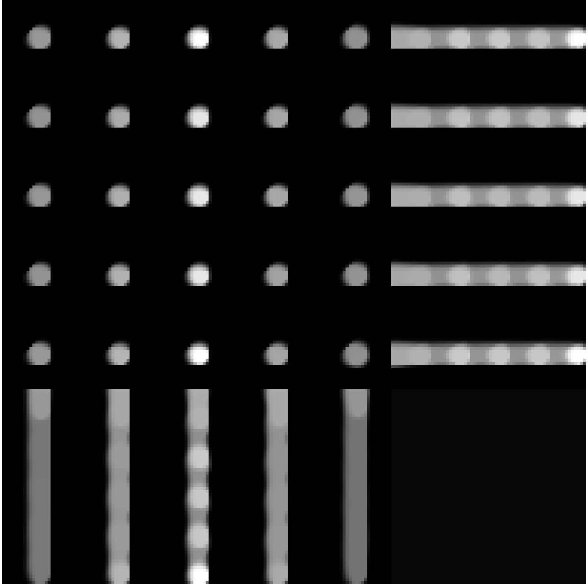
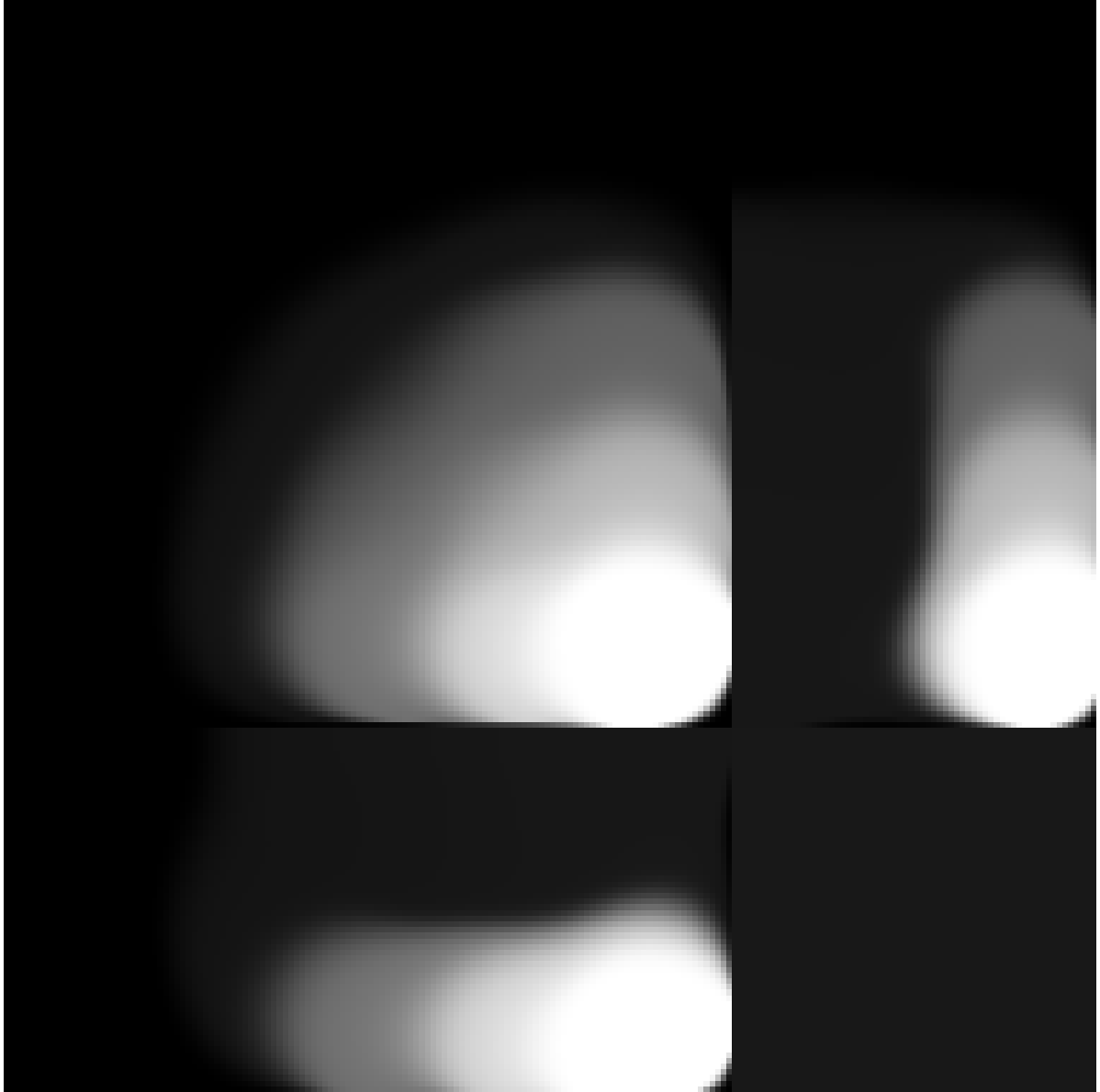
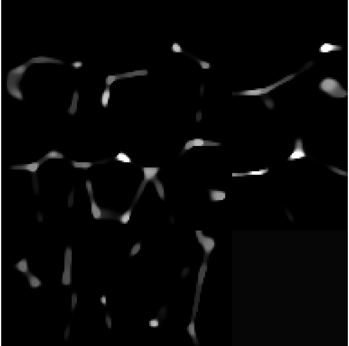
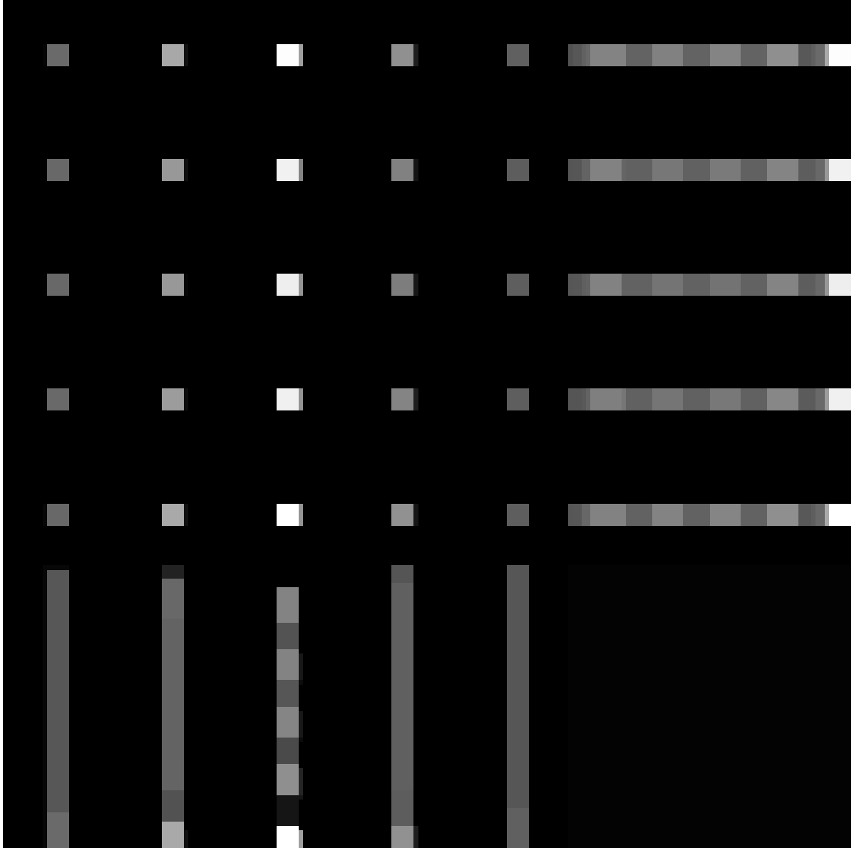
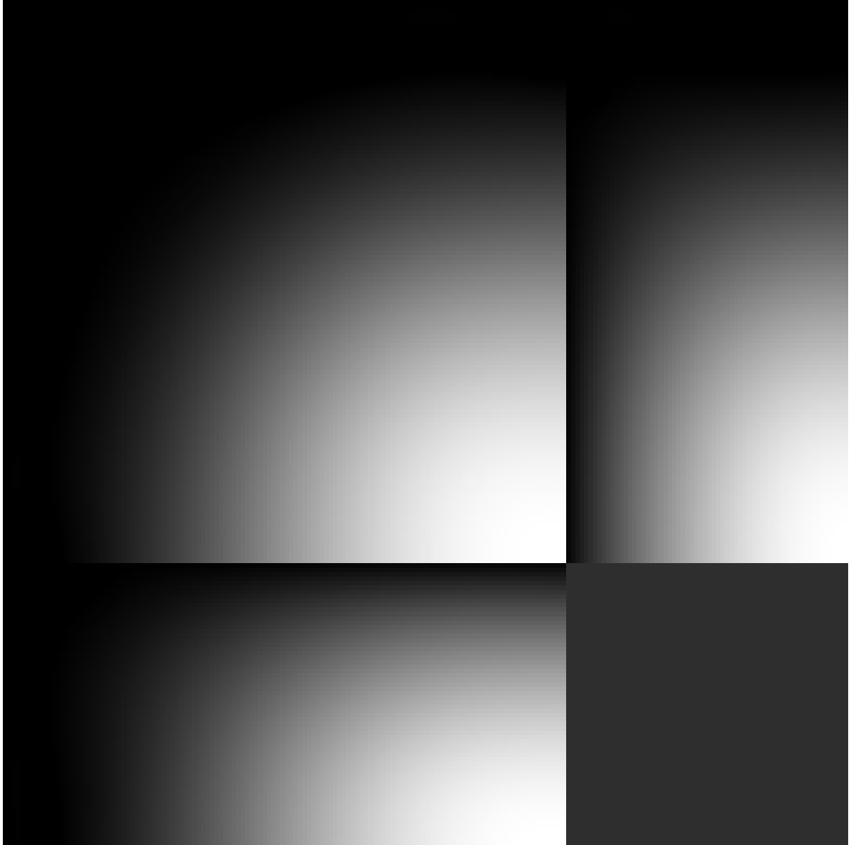
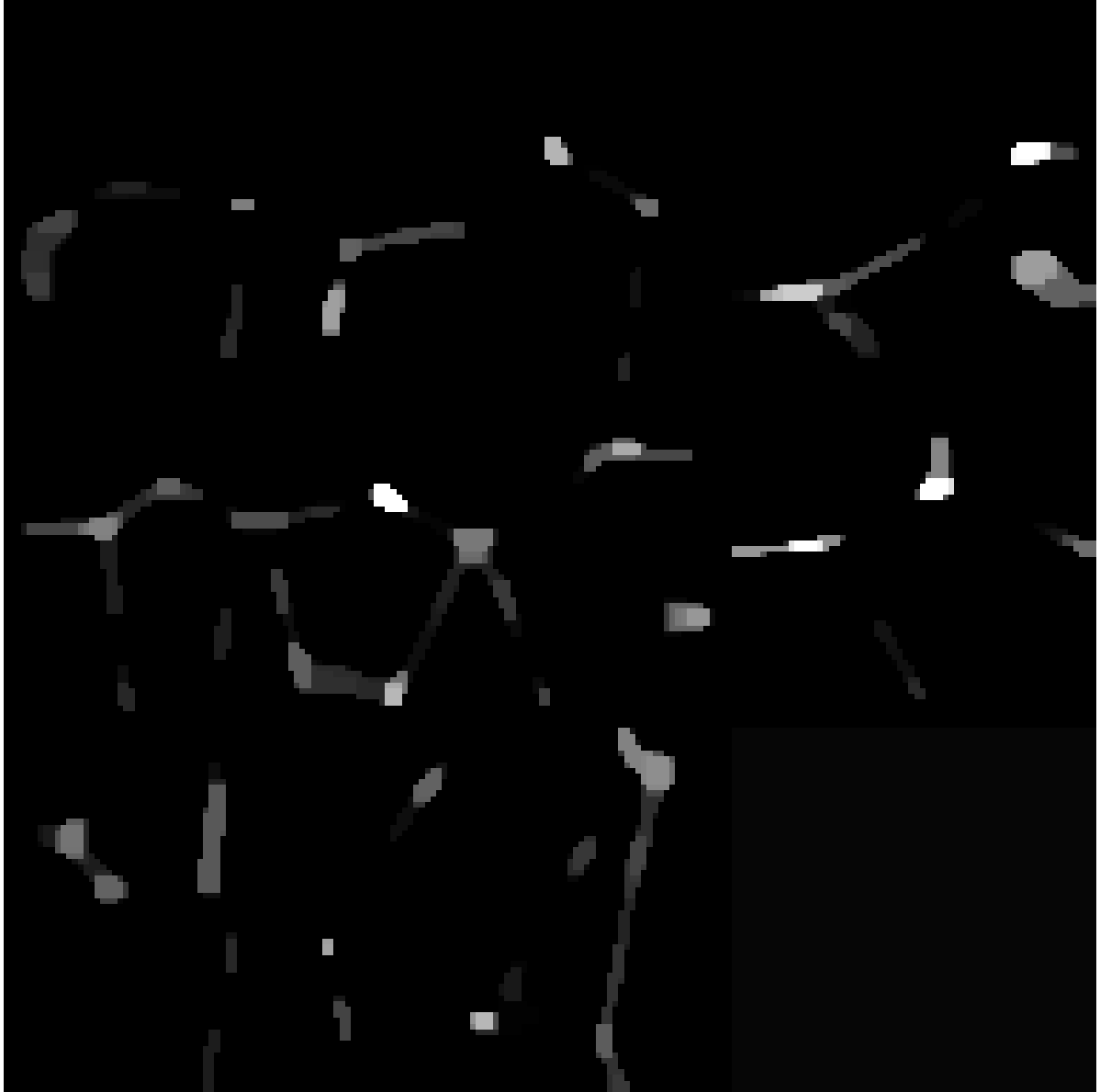
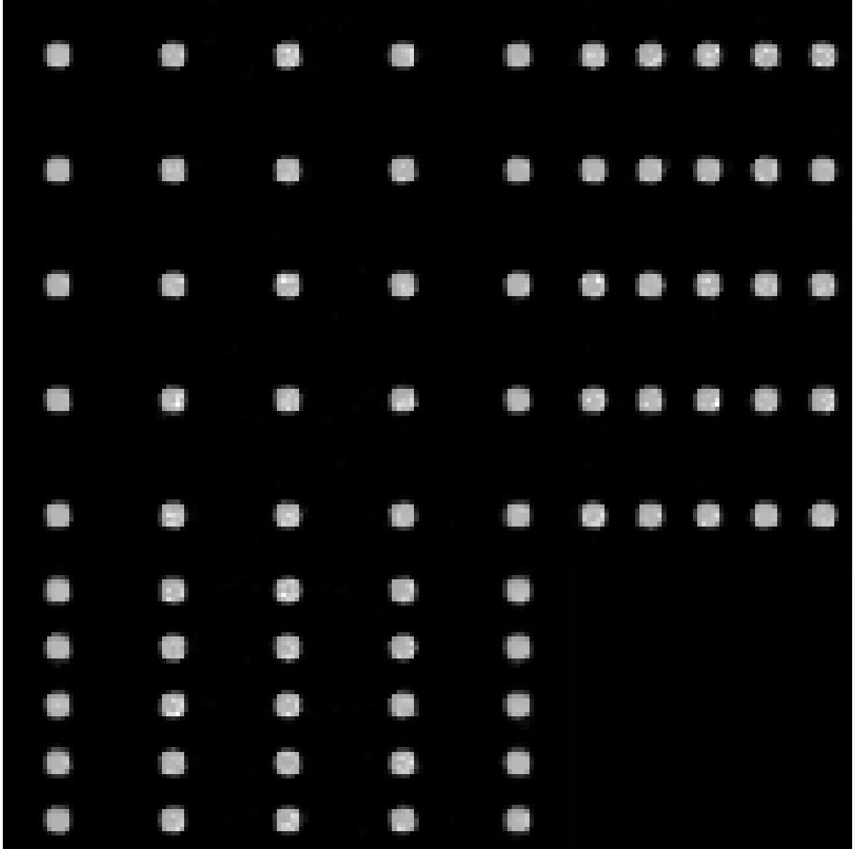
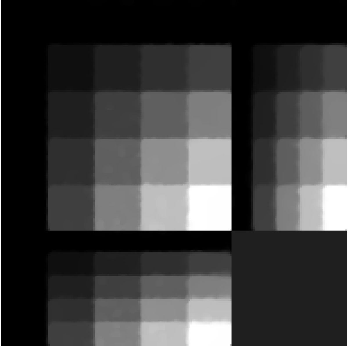
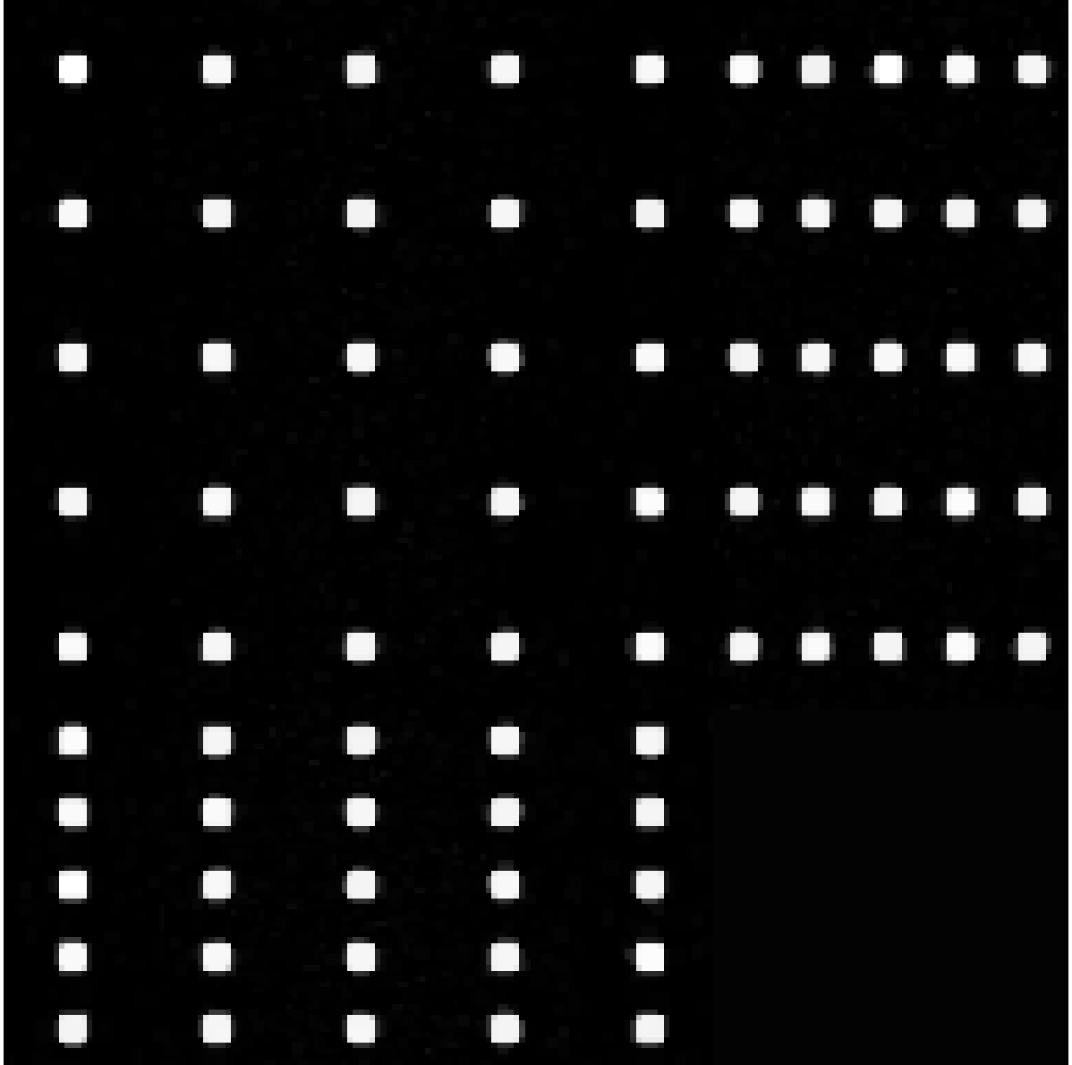
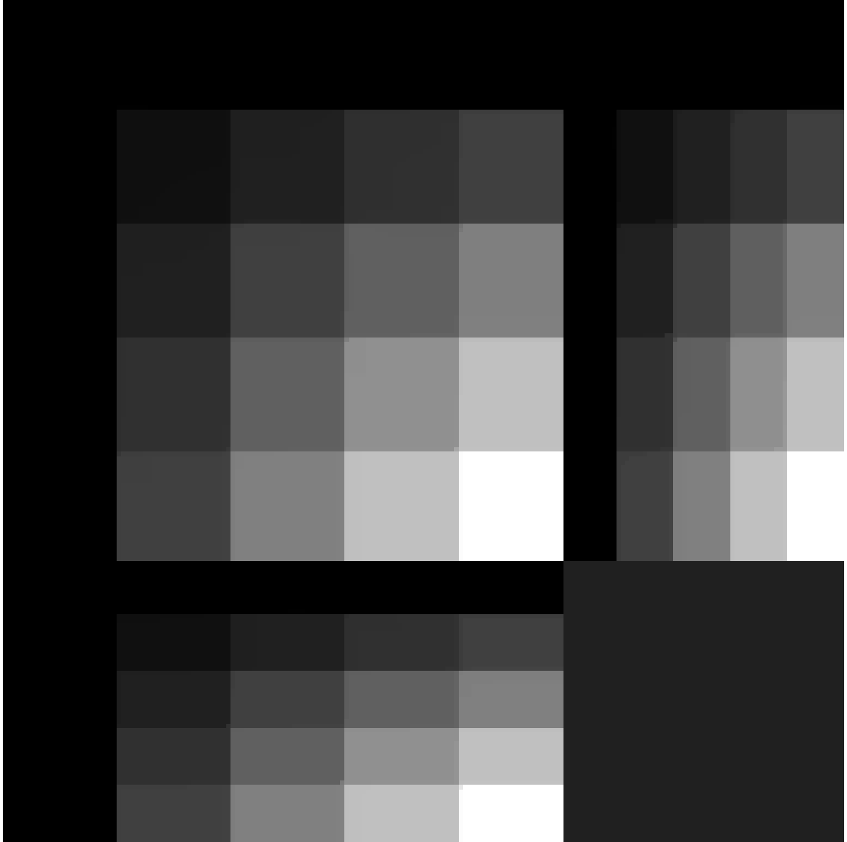
Figure 8: Reconstruction on simulated data with regularisation parameter $\alpha$ such that best MSE is achieved for each method and each image. Shown as maximum intensity projections, except for tissue, where slices in each direction in the centre of the sample are shown. First row: PSF-L2. Second row: PSF-IC. Third row: LS-L2. Fourth row: LS-IC.

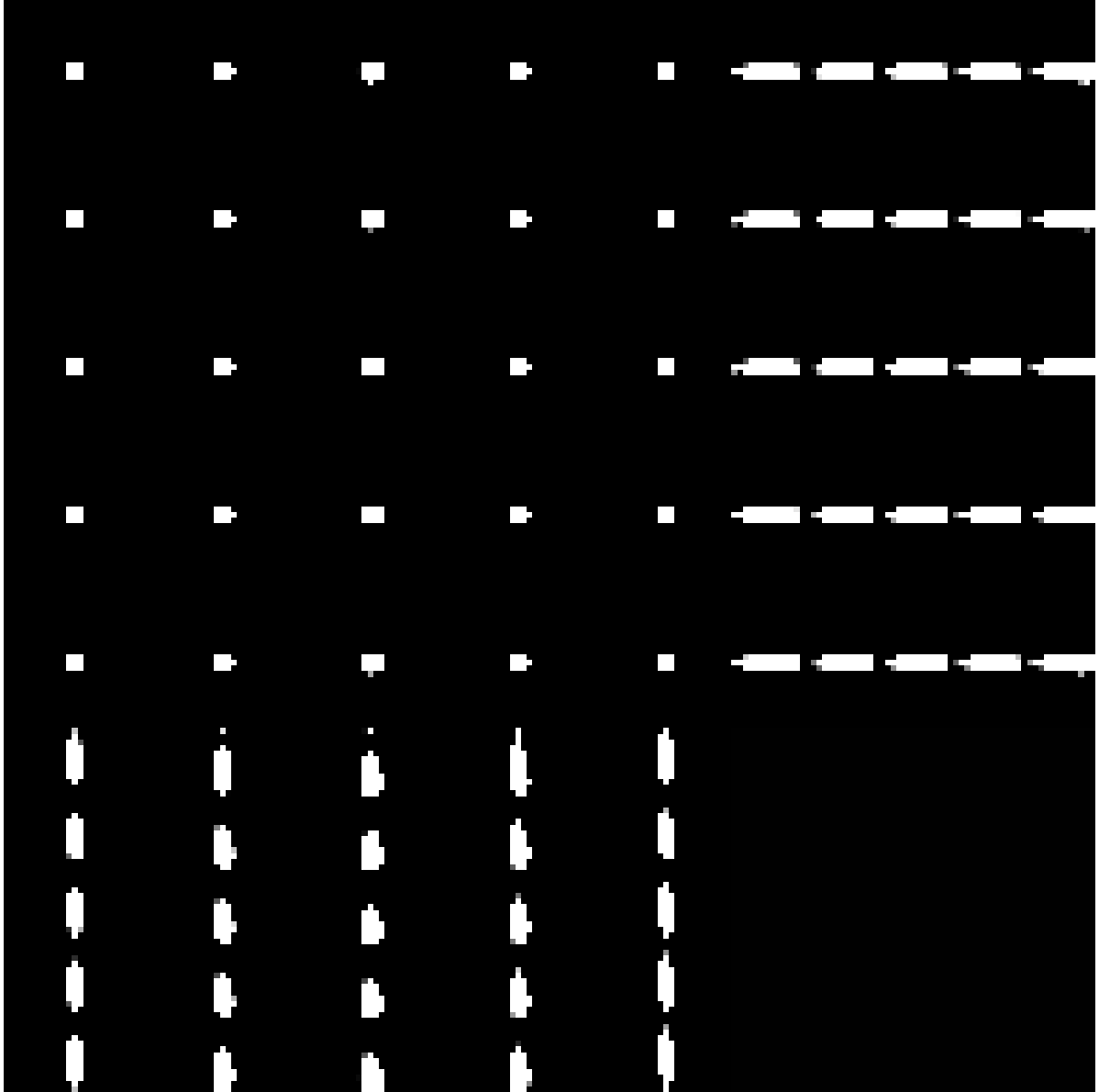
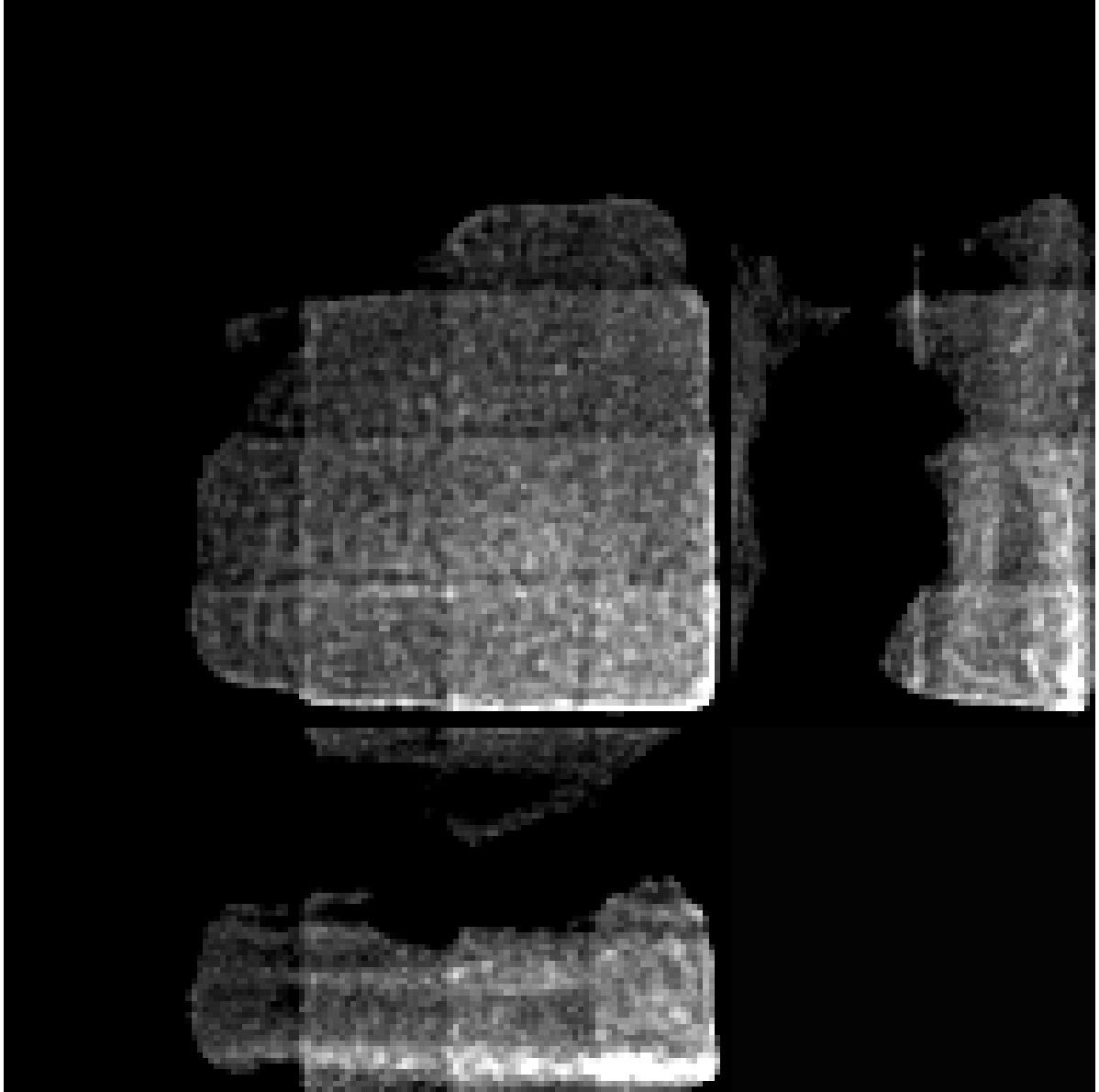
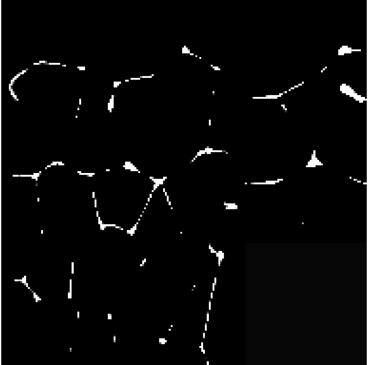
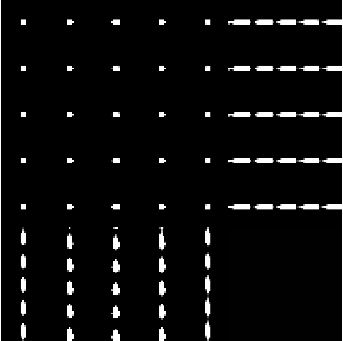
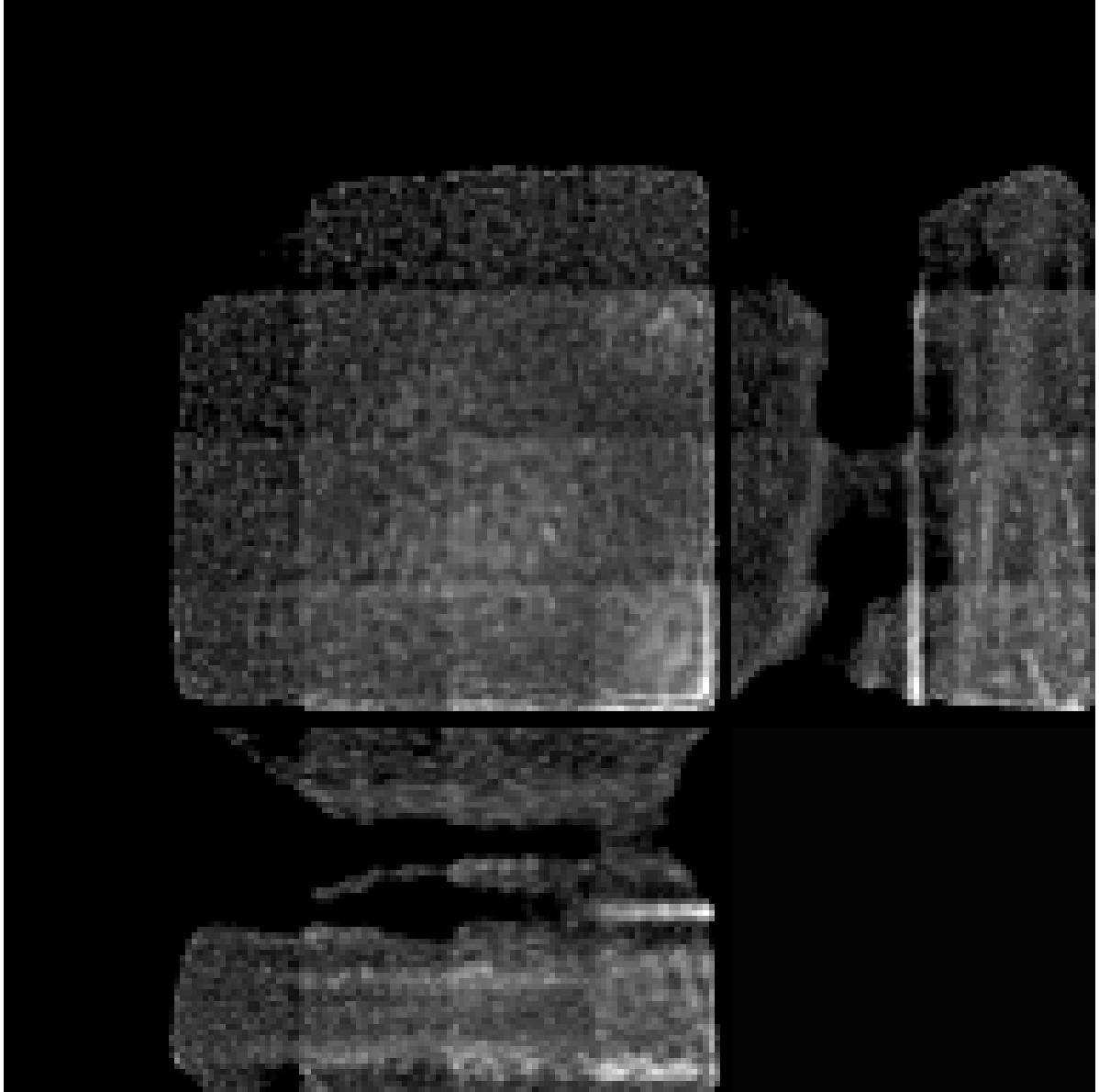
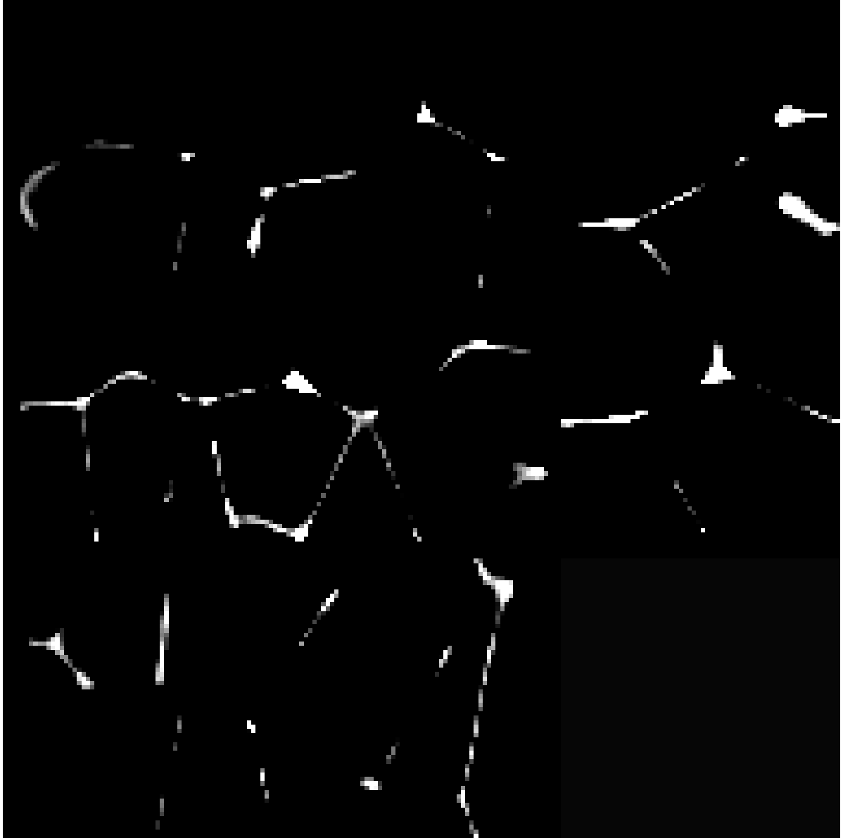
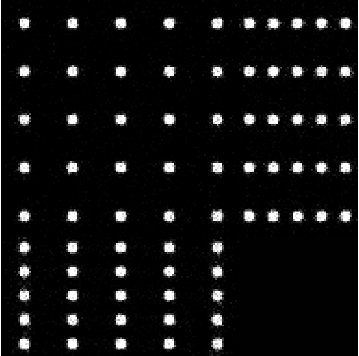
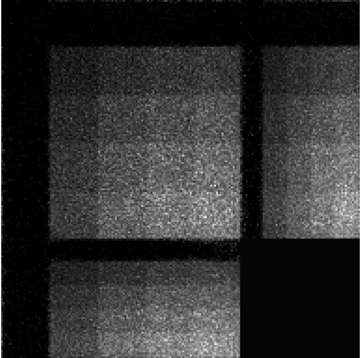
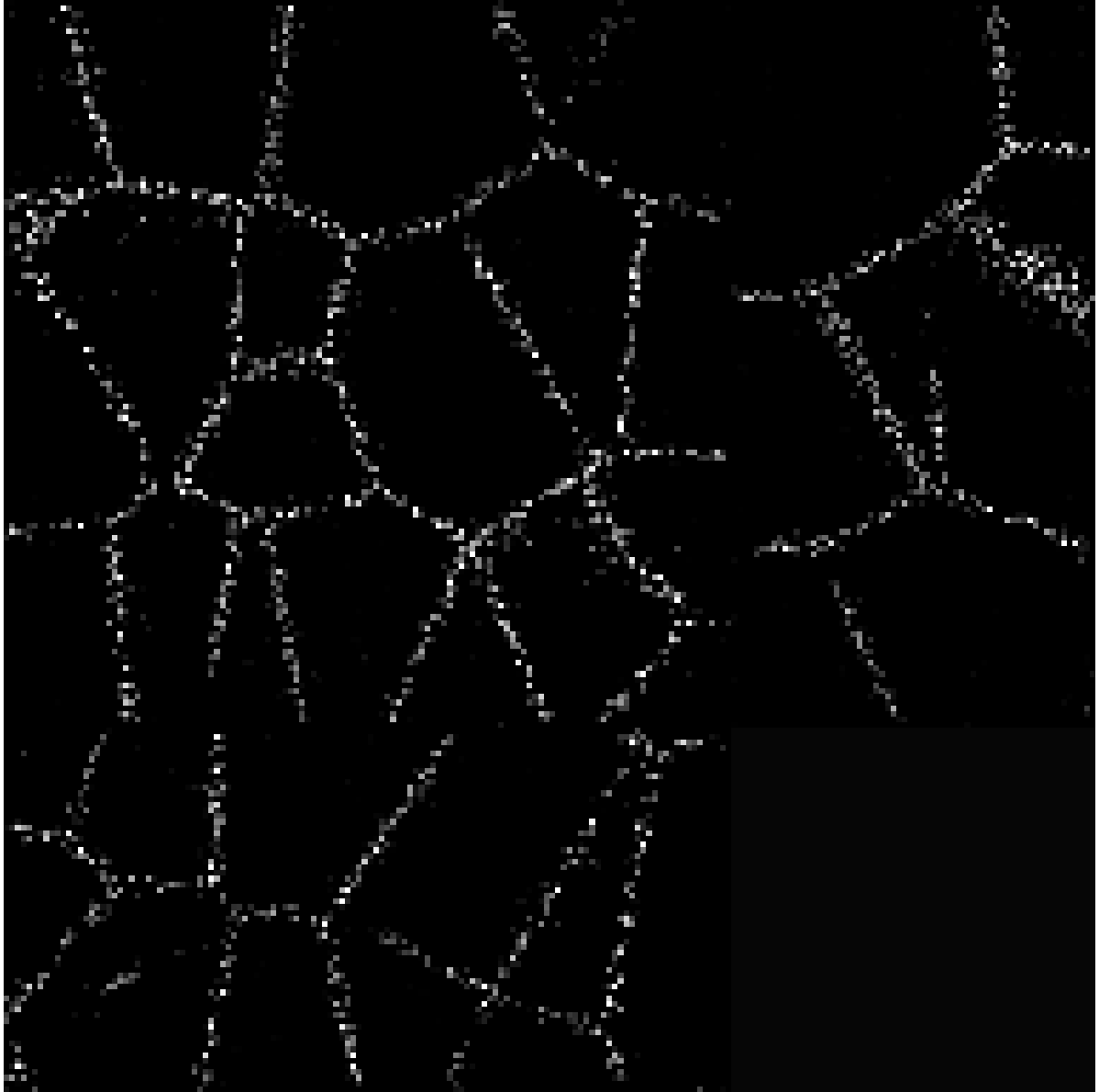
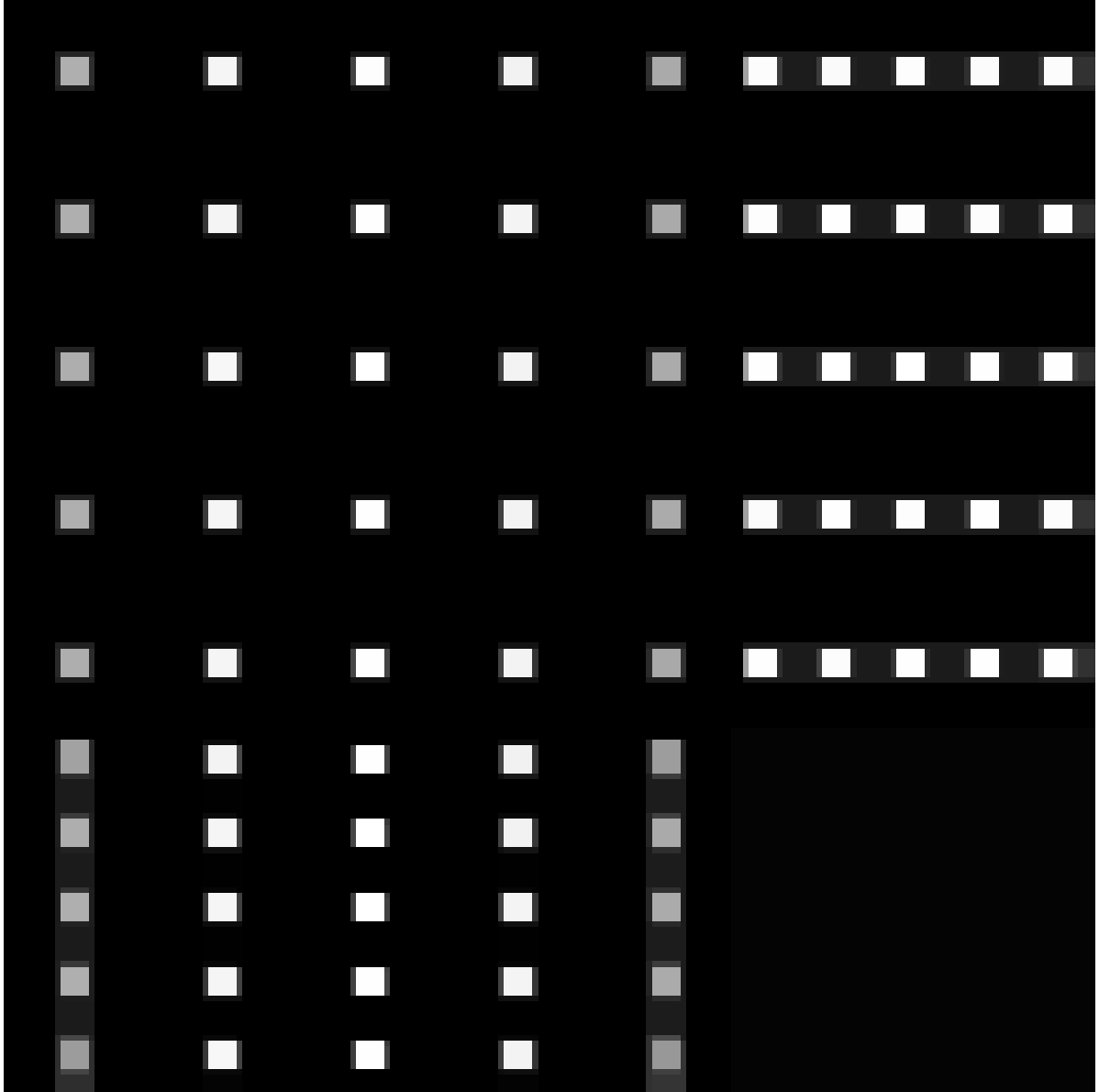
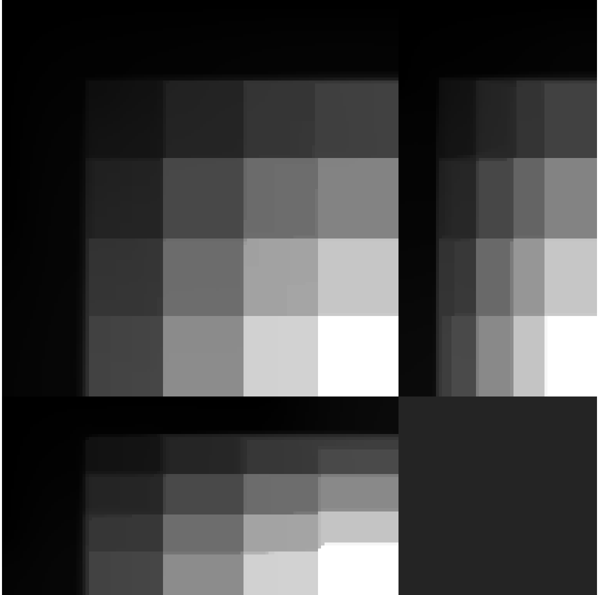
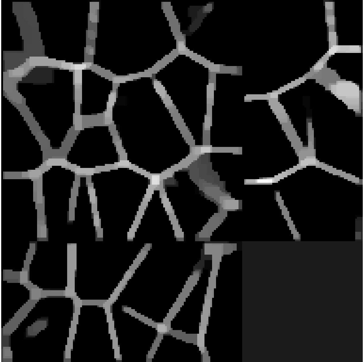
Figure 9: Reconstruction on simulated data with regularisation parameter $\alpha$ chosen to satisfy the discrepancy principle (3.10). Shown as maximum intensity projections, except for tissue, where slices in each direction in the centre of the sample are shown. First row: PSF-L2. Second row: PSF-IC. Third row: LS-L2. Fourth row: LS-IC.

5.2 Light-sheet data

In this section, we show the results of applying LS-IC to a cropped portion of the full resolution images in Figure 2. Specifically, we select a cropped beads image of $1127\times 111\times 100$ voxels and a cropped Marchantia image of $1127\times 156\times 100$ voxels.

For comparison, we also run PSF-L2 on the same images. We run both methods on both images for up to $6000$ iterations, with a normalised primal-dual gap of $10^{-6}$ as a stopping criterion. The parameters for the image formation model used are the same as in Table 2 and the PDHG parameters are given in Table 6.

The results of the deconvolution are shown in Figure 10 and Figure 12 for the beads image and the Marchantia image respectively. In both figures, we first show the position of the light-sheet in the first row (due to the cropping, this is no longer centred), the measured data in the second row, followed by the PSF-L2 reconstruction and the LS-IC reconstruction on the third and fourth row respectively. The regularisation parameter $\alpha$ was chosen in all four cases visually such that a balance is achieved between the amount of regularisation and the noise in the reconstruction.

In the beads image in Figure 10, we note that the LS-IC performs better than PSF-L2 at reversing the effect of the light-sheet. This is most obvious in the $yz$ plane on the right-hand side of the image, where the length of the beads in the $z$ direction has been reduced to a greater extent than in the PSF-L2 reconstruction. In addition, the beads appear less blurry in the LS-IC reconstruction in the right-hand side of the $xy$ plane. We show the bead images in 3D in Figure 11, where the effect of the deconvolution in the $z$ direction is more significant in the LS-IC reconstruction than in the PSF-L2 reconstruction, namely the beads are shorter in $z$. In the Marchantia reconstruction in Figure 12, we see a similar effect of better reconstruction in the $z$ direction, most easily seen in the right-hand side and bottom projections. Moreover, the 3D rendering of the Marchantia sample in Figure 13 shows smoother cell edges in the LS-IC reconstruction, while the PSF-L2 reconstruction contains reconstruction artefacts that are non-existent in the LS-IC reconstruction, indicated by the yellow arrows.

method	LS-IC		PSF-L2
image	beads	Marchantia	beads	Marchantia
$\rho$	0.5	0.7	0.9	0.9
$\sigma$	0.0001	0.0001	0.01	0.001

Table 6: Values of the PDHG parameters $\rho$ and $\sigma$ used in the numerical experiments with real data.

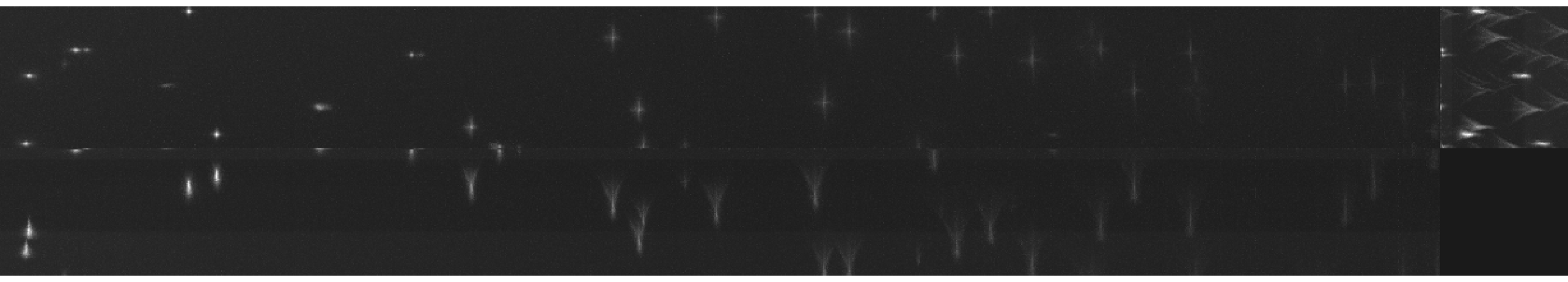
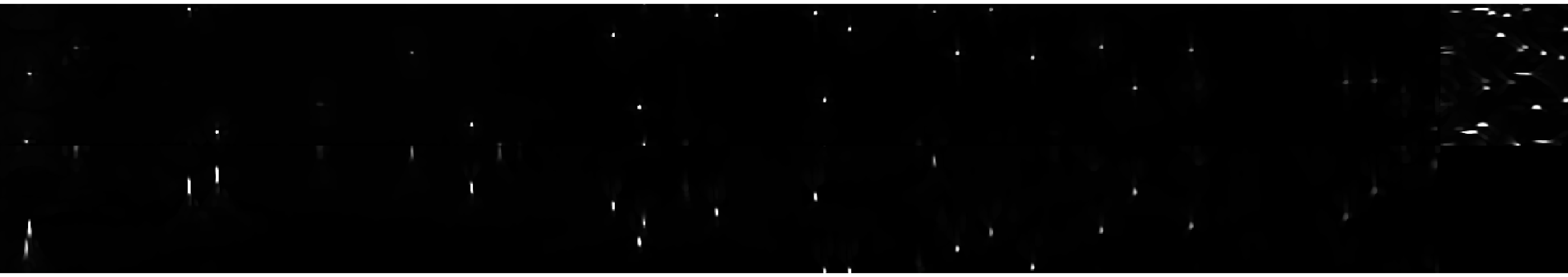
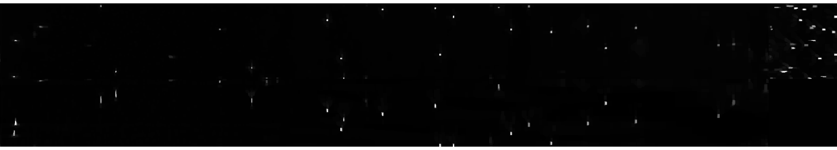
Figure 10: Reconstruction results for the light-sheet bead image, shown as maximum intensity projections. First row: The fitted light-sheet profile. Second row: The data. Third row: PSF-L2 with $\alpha=0.1$. Fourth row: LS-IC with $\alpha=0.0046$.

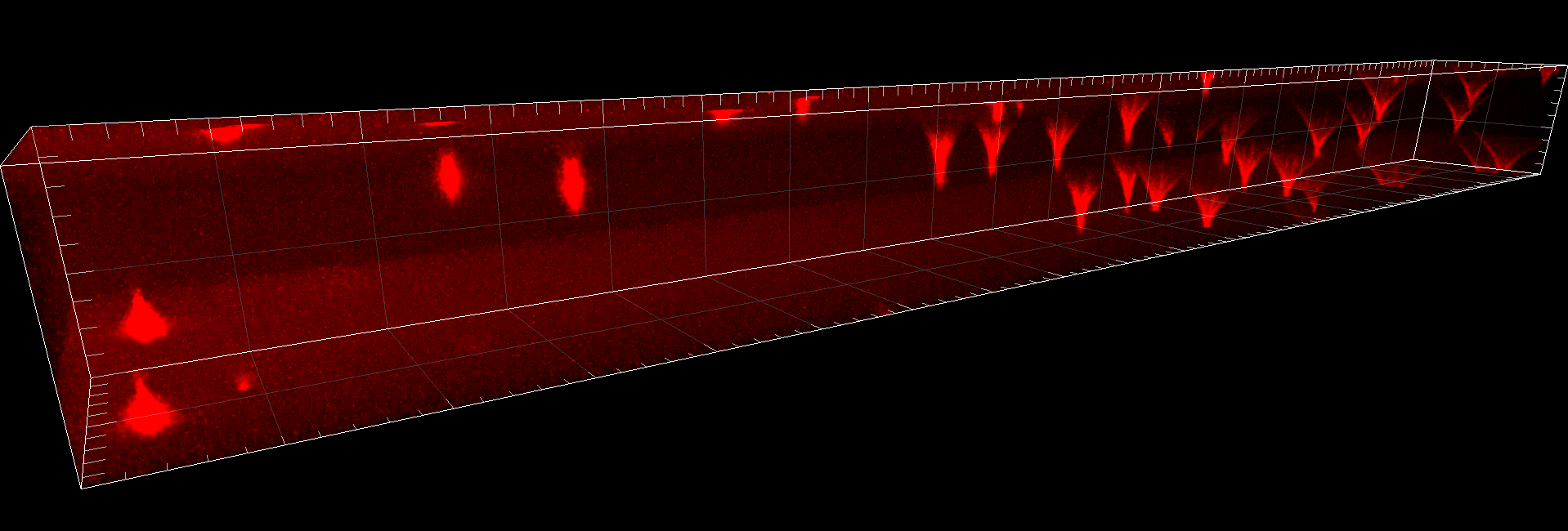
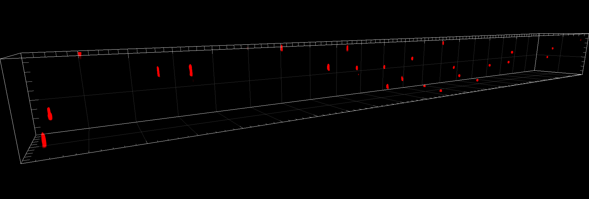
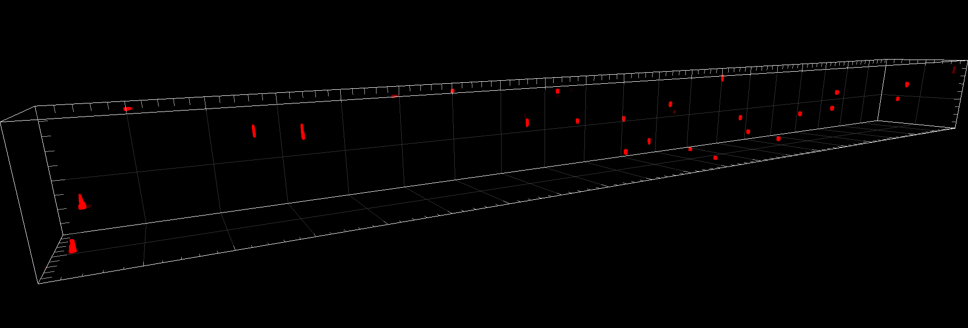
Figure 11: 3D rendering of the beads data and reconstruction images using ImarisViewer 9.7.2. First row: The data. Second row: PSF-L2 with $\alpha=0.1$. Third row: LS-IC with $\alpha=0.0046$.

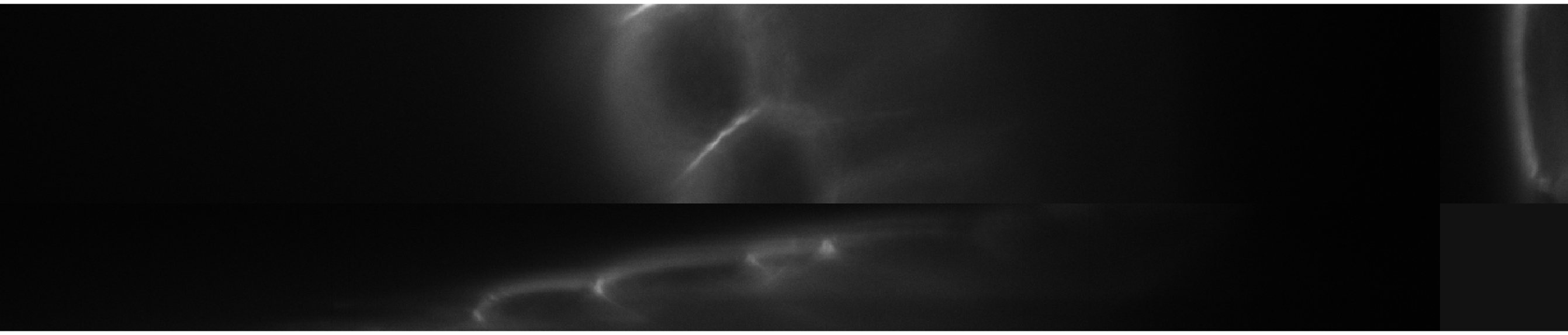
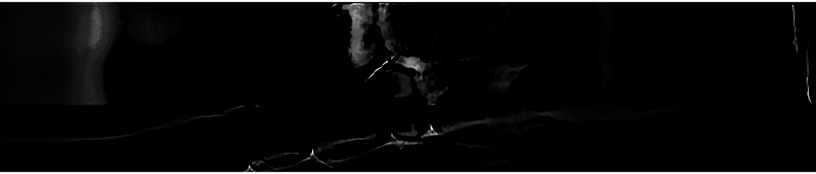
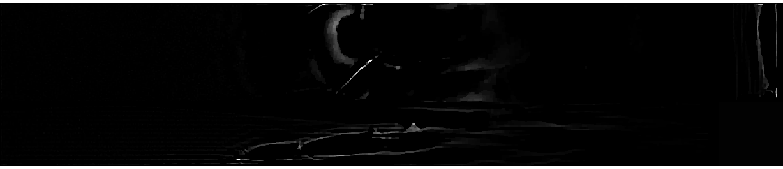
Figure 12: Reconstruction results for the Marchantia sample, shown as slices in each direction in the centre of the sample. First row: The fitted light-sheet profile. Second row: The data. Third row: PSF-L2 with $\alpha=0.1$. Fourth row: LS-IC with $\alpha=0.0005$.

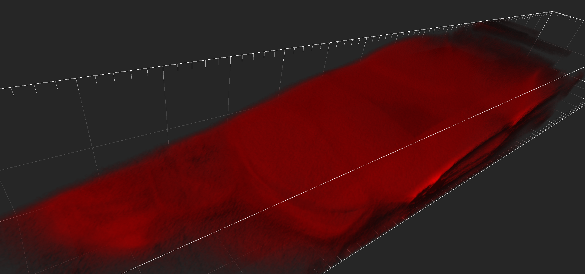
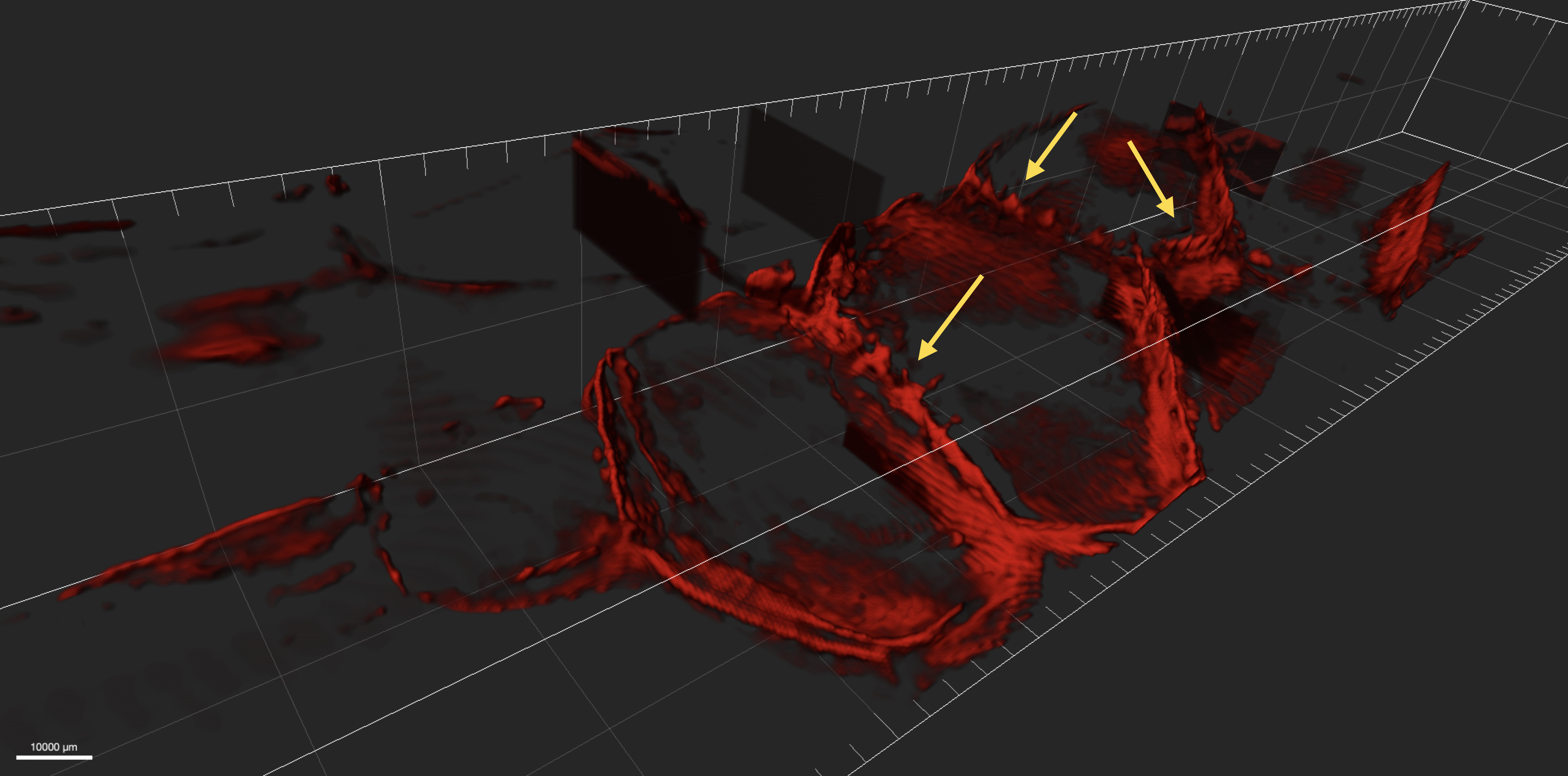
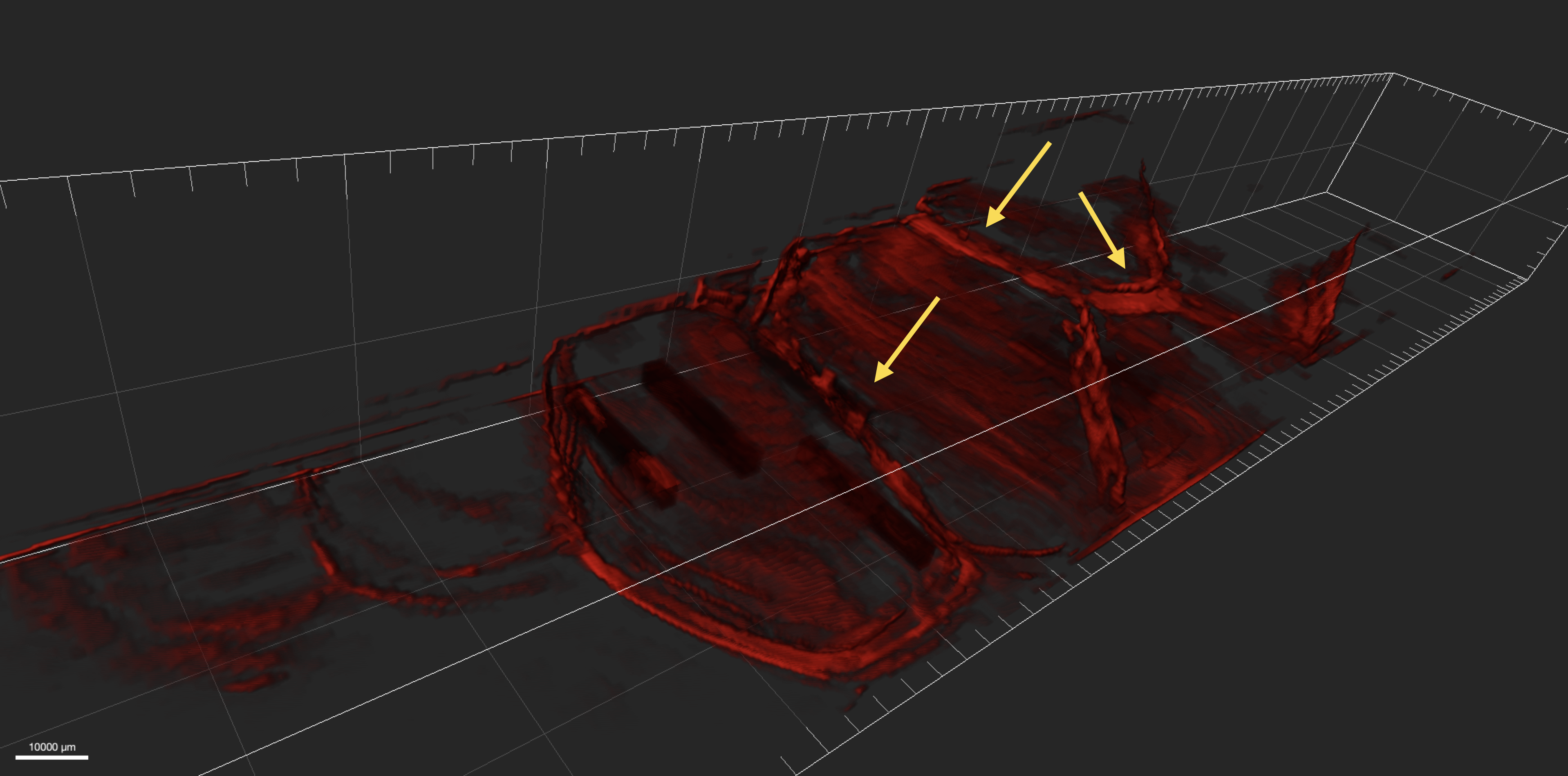
Figure 13: 3D rendering of the Marchantia data and reconstruction images using ImarisViewer 9.7.2. First row: The data. Second row: PSF-L2 with $\alpha=0.1$. Third row: LS-IC with $\alpha=0.0005$.

6 Conclusion

In this paper we introduced a novel method for performing deconvolution for light-sheet microscopy. We start by modelling the image formation process in a way that replicates the physics of a light-sheet microscope, which is achieved by explicitly modelling the interaction of the illumination light-sheet and the detection objective PSF. Moreover, the optical aberrations in the system are modelled using a linear combination of Zernike polynomials in the pupil function of the detection PSF, fitted to bead data using a least squares procedure. We then formulate a variational model taking into account the image formation model as the forward operator and a combination of Poisson and Gaussian noise in the data. The model combines a total variation regularisation term and a fidelity term that is an infimal convolution between an $\operatorname{\mathrm{L}}^{2}$ term and the Kullback-Leibler divergence, introduced in [1]. In addition, we establish convergence rates with respect to the noise and we introduce a discrepancy principle for selecting the regularisation parameter $\alpha$ in the mixed noise setting. We solve the resulting inverse problem by applying the PDHG algorithm in a non-trivial way.

The results in the numerical experiments section show that our method, LS-IC, outperforms simpler approaches to deconvolution of light-sheet microscopy data, where one does not take into account the variability of the overall PSF introduced by the light-sheet excitation, or the combination of Gaussian and Poisson noise. In particular, numerical experiments with simulated data show superior reconstruction quality in terms of the normalised $l^{2}$ error and the structural similarity index, not only by optimising over the regularisation parameter $\alpha$ given the ground truth, but also with an a posteriori choice of $\alpha$ using the stated discrepancy principle. On bead data, the reconstruction obtained using LS-IC shows a more significant reduction of the blur in the $z$ direction compared to PSF-L2, where the light-sheet variations and the Poisson noise are not taken into account. Moreover, reconstruction of a Marchantia sample with LS-IC shows fewer artefacts than the PSF-L2 reconstruction, as well as sharper cell edges and smoother cell membranes.

Future work includes applying this technique to a broader range of samples and using it to answer questions of biological interest. To do so, we see a number of potential future directions that this work can take:

• Adapting the discrepancy principle given in (3.10) for choosing the regularisation parameter $\alpha$ to real data sets, like the ones in Section 5.2.

• Improving the running time of the method potentially by means of randomised approaches.

• Investigating other regularisation terms.

• Making the technique available to other users as a more user-friendly tool.

7 Acknowledgements

BT and LM gratefully acknowledge the funding by Isaac Newton Trust/Wellcome Trust ISSF/University of Cambridge Joint Research Grants Scheme and EPSRC EP/R025398/1. MOL and LM also thank the Gatsby Charitable Foundation for financial support. YK acknowledges financial support of the EPSRC (Fellowship EP/V003615/1), the Cantab Capital Institute for the Mathematics of Information at the University of Cambridge and the National Physical Laboratory. CBS acknowledges support from the Philip Leverhulme Prize, the Royal Society Wolfson Fellowship, the EPSRC grants EP/S026045/1 and EP/T003553/1, EP/N014588/1, EP/T017961/1, the Wellcome Innovator Award RG98755, the Leverhulme Trust project Unveiling the invisible, the European Union Horizon 2020 research and innovation programme under the Marie Skłodowska-Curie grant agreement No. 777826 NoMADS, the Cantab Capital Institute for the Mathematics of Information and the Alan Turing Institute.

Imaging was performed at the Microcopy Facility of the Sainsbury Laboratory Cambridge University. We thank Dr. Alessandra Bonfanti and Dr. Sarah Robinson for providing the Marchantia sample and Prof. Sebastian Schornack and Dr. Giulia Arsuffi (Sainsbury Laboratory Cambridge University) for provision of the line of Marchantia used.

We also acknowledge the support of NVIDIA Corporation with the donation of two Quadro P6000, a Tesla K40c and a Titan Xp GPU used for this research.

References

- [1] Luca Calatroni, Juan Carlos De Los Reyes and Carola-Bibiane Schönlieb “Infimal convolution of data discrepancies for mixed noise removal” In SIAM Journal on Imaging Sciences 10.3 SIAM, 2017, pp. 1196–1233
- [2] “Method of the Year 2014” In Nature methods 12.1, 2015, pp. 1 DOI: 10.1038/nmeth.3251
- [3] James G. McNally, Tatiana Karpova, John Cooper and José Angel Conchello “Three-dimensional imaging by deconvolution microscopy” In Methods: A Companion to Methods in Enzymology 19.3, 1999, pp. 373–385 DOI: 10.1006/meth.1999.0873
- [4] J. L. Starck, E. Pantin and F. Murtagh “Deconvolution in Astronomy: A Review” In Publications of the Astronomical Society of the Pacific 114.800, 2002, pp. 1051–1069 DOI: 10.1086/342606
- [5] P. Sarder and A. Nehorai “Deconvolution methods for 3-D fluorescence microscopy images” In IEEE Signal Processing Magazine 23.3, 2006, pp. 32–45
- [6] Antonin Chambolle and Thomas Pock “An introduction to continuous optimization for imaging” In Acta Numerica 25, 2016, pp. 161–319
- [7] Loïc Denis et al. “Fast Approximations of Shift-Variant Blur” In International Journal of Computer Vision 115.3 Springer Verlag, 2015, pp. pp 253–278 DOI: 10.1007/s11263-015-0817-x
- [8] Valentin Debarnot, Paul Escande and Pierre Weiss “A scalable estimator of sets of integral operators” In Inverse Problems 35.10 IOP Publishing, 2019, pp. 105011 DOI: 10.1088/1361-6420/ab2fb3
- [9] James G. Nagy and Dianne P. O’Leary “Restoring images degraded by spatially variant blur” In SIAM Journal of Scientific Computing 19.4, 1998, pp. 1063–1082 DOI: 10.1137/S106482759528507X
- [10] Saima Ben Hadj, Laure Blanc-Féraud and Gilles Aubert “Space variant blind image restoration” In SIAM Journal on Imaging Sciences 7.4, 2014, pp. 2196–2225 DOI: 10.1137/130945776
- [11] M. Hirsch, S. Sra, B. Schölkopf and S. Harmeling “Efficient Filter Flow for Space-Variant Multiframe Blind Deconvolution” In Proceedings of the 23rd IEEE Conference on Computer Vision and Pattern Recognition Piscataway, NJ, USA: IEEE, 2010, pp. 607–614 Max-Planck-Gesellschaft
- [12] Daniel O’Connor and Lieven Vandenberghe “Total variation image deblurring with space-varying kernel” In Computational Optimization and Applications 67.3, 2017, pp. 521–541 DOI: 10.1007/s10589-017-9901-1
- [13] Maja Temerinac-Ott et al. “Multiview deblurring for 3-D images from light-sheet-based fluorescence microscopy” In IEEE Transactions on Image Processing 21.4, 2012, pp. 1863–1873 DOI: 10.1109/TIP.2011.2181528
- [14] Stephan Preibisch et al. “Efficient Bayesian-based multiview deconvolution” In Nature Methods 11.6, 2014, pp. 645–648 DOI: 10.1038/nmeth.2929
- [15] Klaus Becker et al. “Deconvolution of light sheet microscopy recordings” In Scientific Reports 9.1, 2019, pp. 1–14 DOI: 10.1038/s41598-019-53875-y
- [16] Min Guo et al. “Rapid image deconvolution and multiview fusion for optical microscopy” In Nature Biotechnology, 2020 DOI: 10.1038/s41587-020-0560-x
- [17] Zhe Zhang et al. “3D Hessian deconvolution of thick light-sheet z-stacks for high-contrast and high-SNR volumetric imaging” In Photon. Res. 8.6 OSA, 2020, pp. 1011–1021 DOI: 10.1364/PRJ.388651
- [18] Evelyn Cueva et al. “Mathematical modeling for 2D light-sheet fluorescence microscopy image reconstruction” In Inverse Problems 36.7 IOP Publishing, 2020, pp. 075005 DOI: 10.1088/1361-6420/ab80d8
- [19] Jie Zhang et al. “Bilinear constraint based ADMM for mixed Poisson-Gaussian noise removal” In Inverse Problems & Imaging 15.2, 2021, pp. 339–366
- [20] A. Stokseth “Properties of a Defocused Optical System” In J Opt Soc Amer 59.10, 1969, pp. 1314–1321 DOI: 10.1364/josa.59.001314
- [21] Ferréol Soulez, Eric T. Hiébaut, Yves T. Ourneur and Loïc D. Enis “Déconvolution aveugle en microscopie de fluorescence 3D” In GRETSI, 2013
- [22] Alan M. Dunn, Owen S. Hofmann, Brent Waters and Emmett Witchel “Cloaking malware with the trusted platform module” In Proceedings of the 20th USENIX Security Symposium, 2011, pp. 395–410
- [23] B. M. Hanser, M. G.L. Gustafsson, D. A. Agard and J. W. Sedat “Phase-retrieved pupil functions in wide-field fluorescence microscopy” In Journal of Microscopy 216.1, 2004, pp. 32–48 DOI: 10.1111/j.0022-2720.2004.01393.x
- [24] Richard G. Paxman, Timothy J. Schulz and James R. Fienup “Joint estimation of object and aberrations by using phase diversity” In Journal of the Optical Society of America A 9.7, 1992, pp. 1072 DOI: 10.1364/josaa.9.001072
- [25] Petar N. Petrov, Yoav Shechtman and W. E. Moerner “Measurement-based estimation of global pupil functions in 3D localization microscopy” In Optics Express 25.7, 2017, pp. 7945 DOI: 10.1364/oe.25.007945
- [26] James C. Wyant and Katherine Creath “Basic Wavefront Aberration Theory for Optical Metrology” In Applied Optics and Optical Engineering, Volume XI New York: Academic Press, 1992, pp. 11–53
- [27] Martin Burger and Stanley Osher “A guide to the TV zoo” In Level-Set and PDE-based Reconstruction Methods Springer, 2013
- [28] Thorsten Hohage and Frank Werner “Iteratively regularized Newton-type methods for general data misfit functionals and applications to Poisson data” In Numerische Mathematik 123.4, 2013, pp. 745–779 DOI: 10.1007/s00211-012-0499-z
- [29] Thorsten Hohage and Frank Werner “Inverse problems with Poisson data: statistical regularization theory, applications and algorithms” In Inverse Problems 32.9 IOP Publishing, 2016, pp. 093001 DOI: 10.1088/0266-5611/32/9/093001
- [30] Alessandro Lanza, Serena Morigi, Fiorella Sgallari and You-Wei Wen “Image restoration with Poisson–Gaussian mixed noise” In Comput Methods Biomech Biomed Eng Imaging Vis 2, 2014, pp. 12–24
- [31] Christian Clason, Dirk A. Lorenz, Hinrich Mahler and Benedikt Wirth “Entropic regularization of continuous optimal transport problems” In Journal of Mathematical Analysis and Applications 494.1, 2021, pp. 124432 DOI: https://doi.org/10.1016/j.jmaa.2020.124432
- [32] C. Bennett and R. Sharpley “Interpolation of Operators” 129, Pure and Applied Mathematics Boston MA: Academic Press, 1988
- [33] Heinz H. Bauschke and Patrick L. Combettes “Convex Analysis and Monotone Operator Theory in Hilbert Spaces” Springer, 2011
- [34] Leonid I. Rudin, Stanley Osher and Emad Fatemi “Nonlinear total variation based noise removal algorithms” In Physica D: Nonlinear Phenomena 60.1, 1992, pp. 259 –268 DOI: 10.1016/0167-2789(92)90242-F
- [35] Martin Benning and Martin Burger “Modern Regularization Methods for Inverse Problems” In Acta Numerica 27, 2018, pp. 1–111
- [36] Martin Burger and Stanley Osher “Convergence rates of convex variational regularization” In Inverse Problems 20.5, 2004, pp. 1411 URL: http://stacks.iop.org/0266-5611/20/i=5/a=005
- [37] Elena Resmerita and Robert S. Anderssen “Joint additive Kullback–Leibler residual minimization and regularization for linear inverse problems” In Mathematical Methods in the Applied Sciences 30.13, 2007, pp. 1527–1544 DOI: https://doi.org/10.1002/mma.855
- [38] Leon Bungert, Martin Burger, Yury Korolev and Carola-Bibiane Schönlieb “Variational regularisation for inverse problems with imperfect forward operators and general noise models” In Inverse Problems 36.12 IOP Publishing, 2020, pp. 125014 DOI: 10.1088/1361-6420/abc531
- [39] V. A. Morozov “On the solution of functional equations by the method of regularisation” In Soviet Math. Dokl. 7, 1966, pp. 414–417
- [40] H. W. Engl, M. Hanke and A. Neubauer “Regularization of Inverse Problems” Springer, 1996
- [41] Bruno Sixou, Tom Hohweiller and Nicolas Ducros “Morozov principle for Kullback-Leibler residual term and Poisson noise” In Inverse Problems & Imaging 12.3, 2018, pp. 607–634 DOI: 10.3934/ipi.2018026
- [42] Göran Lindblad “Entropy, information and quantum measurements” In Communications in Mathematical Physics 33.4, 1973, pp. 305–322 DOI: 10.1007/BF01646743
- [43] Ernie Esser, Xiaoqun Zhang and Tony F Chan “A general framework for a class of first order primal-dual algorithms for convex optimization in imaging science” In SIAM Journal on Imaging Sciences 3.4 SIAM, 2010, pp. 1015–1046
- [44] Antonin Chambolle and Thomas Pock “A first-order primal-dual algorithm for convex problems with applications to imaging” In Journal of mathematical imaging and vision 40.1 Springer, 2011, pp. 120–145
- [45] Laurent Condat “A primal-dual splitting method for convex optimization involving Lipschitzian, proximable and linear composite terms” In Journal of Optimization Theory and Applications 158.2 Springer, 2013, pp. 460–479
- [46] Riccardo Zanella, Patrizia Boccacci, Luca Zanni and Mario Bertero “Efficient gradient projection methods for edge-preserving removal of Poisson noise” In Inverse Problems 25.4 IOP Publishing, 2009, pp. 045010 DOI: 10.1088/0266-5611/25/4/045010