Neighborhood Consensus Contrastive Learning for Backward-Compatible Representation

Abstract

In object re-identification (ReID), the development of deep learning techniques often involves model updates and deployment. It is unbearable to re-embedding and re-index with the system suspended when deploying new models. Therefore, backward-compatible representation is proposed to enable “new” features to be compared with “old” features directly, which means that the database is active when there are both “new” and “old” features in it. Thus we can scroll-refresh the database or even do nothing on the database to update.

The existing backward-compatible methods either require a strong overlap between old and new training data or simply conduct constraints at the instance level. Thus they are difficult in handling complicated cluster structures and are limited in eliminating the impact of outliers in old embeddings, resulting in a risk of damaging the discriminative capability of new features. In this work, we propose a Neighborhood Consensus Contrastive Learning (NCCL) method. With no assumptions about the new training data, we estimate the sub-cluster structures of old embeddings. A new embedding is constrained with multiple old embeddings in both embedding space and discrimination space at the sub-class level. The effect of outliers diminished, as the multiple samples serve as “mean teachers”. Besides, we also propose a scheme to filter the old embeddings with low credibility, further improving the compatibility robustness. Our method ensures backward compatibility without impairing the accuracy of the new model. And it can even improve the new model’s accuracy in most scenarios.

1 Introduction

General object re-identification (ReID) aims at finding a significant person/vehicle of interest in a large amount of collection, called “gallery”. It has attracted much interest in computer vision due to its great contributions in urban surveillance and intelligent transportation [34, 15]. Specifically, existing ReID methods typically map each image into vector space using a convolutional neural network. The output in vector space is usually called “embedding”. Given query images of a specific object, the process of ReID is to find the same identity in the gallery by finding its nearest neighbors in embedding space.

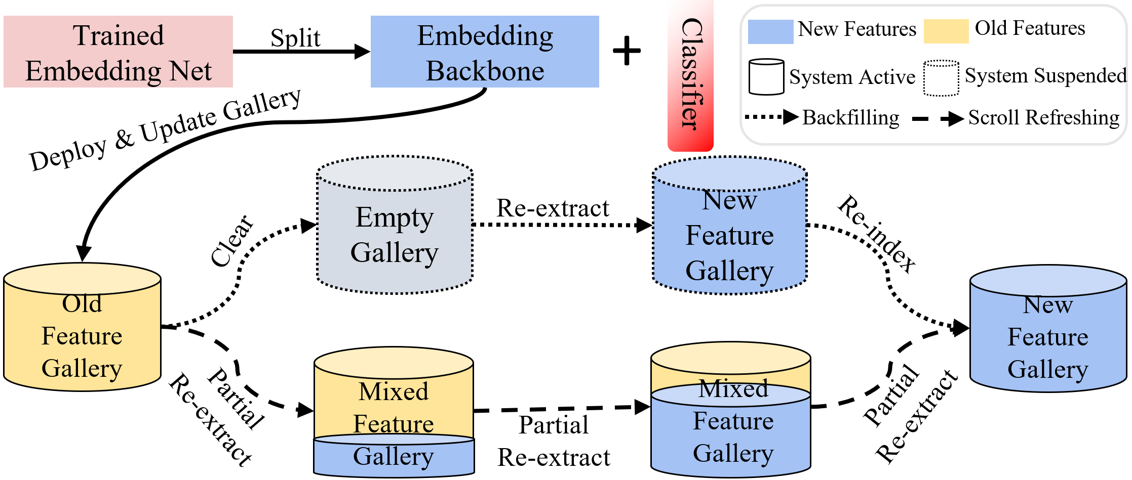
Figure 1: The Deployment Process. Without backward compatibility, the process to update the gallery is “backfilling” with the system suspended until re-index has been done. With backward compatibility, the process to update is “scroll refreshing” with the system always active. Notice that the classifier is abandoned when deployed as it is useless for retrieval but only a waste of space. Thus the old classifier is unavailable when the old model is from a third party.

As the new training data or the improved model designs are available, the deployed model will be updated to a new version with better performance. Then we need to refresh the gallery to harvest the benefits of the new model, namely “backfilling”. As it is common to have millions or even billions of images in the database/gallery [21], backfilling is a painful process, which requires re-extracting embeddings and re-building indexes with the system suspended, as shown in Figure 1. An ideal solution is enabling “new” embeddings to be compared with “old” embeddings directly. Then we can gradually replace “old” embedding with “new” embeddings in the gallery while the system is still active, named “scroll refreshing”. What’s more, if the gallery is in scroll-refreshed mode initially (e.g., only keep the surveillance data in the past $x$ days), the proportion of new embeddings in the gallery increases from 0% to 100% over some time automatically.

To achieve backfilling-free, backward-compatible representation learning methods have recently arisen. Under a backward-compatible setting, given an anchor sample from new embeddings, no matter the positives and negatives from old/new embeddings, the anchor is consistently closer to the positives than the negatives. Recently, metric learning methods are adopted to optimize the distances between new and old embeddings in an asymmetric way [3]. However, the adopted pair-based triplet losses can not well consider the feature cluster structure differences across different embeddings. They are sensitive to the outliers in the old embeddings and hard to convergence on the large-scale dataset. Alternatively, the classifier of the old model is used to regularize the new embeddings in training the new model [22], termed as “backward-compatible training (BCT)”. The old classifier is based on a weight matrix, where each column can be viewd as a “prototype” of a particular class in old training sets. Such prototype is also limited in characterizing the cluster structure. What’s more, BCT can only work when the new and old training sets have common classes and the old classifier is available.

The old embedding space is often not ideal and faces complicated cluster structures. For example, due to the intra-class variance caused by varied postures, colors, viewpoints, and lighting conditions, the cluster structure often tends to be scattered as multiple sub-clusters. Moreover, the old embedding space also inevitably contains some noise data and outliers in clusters. Simply constraining the learned “anchor” of new embeddings close to the randomly sampled “fixed positives” of old embeddings has a risk of damaging the discriminative capability of new embeddings. Therefore, it is necessary to consider the entire cluster structure across new and old embeddings in backward-compatible learning.

In this work, we propose a Neighborhood Consensus Contrastive Learning (NCCL) method for backward-compatible representation. Previous methods mainly constrain the distributions of the new embeddings to be consistent with the old. We design a supervised contrastive learning method to constrain the distance relationship between the new and old embeddings to be consistent. Specifically, we estimate the sub-cluster structures in old embeddings. A new embedding is constrained by multiple old embeddings from different sub-clusters. The priorities of different sub-clusters are carefully designed to dominate the optimizing progress. Also, the effect of outliers in old embeddings diminished, as the multiple old embeddings serve as “mean teachers” and the outliers contribute little during the optimizing progress. Typically, the classifier head in a network converts the embedding space to discrimination space for classification. Therefore, the discrimination space contains rich class-level information [40]. Correspondingly, we further design a soft multi-label task to exploit such knowledge to enhance compatible learning. Such labels are an auxiliary apart from the real-word labels, making the new embeddings more discriminative. Besides, since the quality of the old model is unpredictable, we estimate the entropy distribution of the old embeddings and remove the ones with low credibility. It helps to maintain robustness when learning backward-compatible representation from old models with various qualities.

Our contributions are summarized as follows:

• We propose a Neighborhood Consensus Contrastive Learning (NCCL) method for backward-compatible representation. With no assumptions about the new training data, we start from a neighborhood consensus perspective, and constrain at the sub-cluster level to keep the discriminative capability of new embeddings. The impact of outliers is reduced as they contribute little to such optimizing progress.

• We perform backward-compatible learning from both embedding space and discrimination space, with priorities of different sub-clusters dominating the optimizing progress. We further propose a novel scheme to filter the old embeddings with low credibility, which is helpful to maintain robustness with the qualities of old models various.

• The proposed method obtains state-of-the-art performance on the evaluated benchmark datasets. We can ensure backward compatibility without impairing the accuracy of the new model. In most cases, it even improves the accuracy of the new model.

2 Related work

2.1 Object re-identification

Object re-identification can realize cross-camera image retrieval, tracking, and trajectory prediction of pedestrians or vehicles. In recent years, research in this field has mainly focused on network architecture design [26, 44], feature representation learning [38, 32], deep metric learning [29, 5, 42], ranking optimization [33, 1], and recognition under video sequences [14, 10, 16]. Deep metric learning aims to establish similarity/dissimilarity between images. This paper is to design based on the metric learning paradigms and establish similarity/dissimilarity between new and old embeddings, aiming to learn backward-compatible representation.

2.2 Backward-compatible representation

Backward-compatible learning encourages the new embeddings closer to the old embeddings with the same class ID than that with different class IDs. It is an emerging topic. To the best of our knowledge, there only exist two pieces of research. Budnik et al. [3] adopts the metric learning loss, e.g., triplet loss and contrastive loss, in an asymmetric way to achieve backward-compatible learning. We call this method “Asymmetric” for convenience. Shen et al. [22] proposes BCT, a backward-compatible representation learning model. BCT feeds the new embeddings into the old classifier. Then the output logits are optimized with cross-entropy loss. BCT and Asymmetric are essentially identical, as it is equivalent to a smoothed triplet loss where each old embedding class has a single center [20]. With the newly added data, BCT needs to use knowledge distillation techniques. In general, existing methods simply adopt embedding losses or classification losses in an asymmetric way. However, such loss is limited in handling the complicated cluster structures of fixed old embeddings. In this article, we consider this problem from a neighborhood consensus perspective with both embedding structure and discrimination knowledge.

2.3 Contrastive learning

Contrastive learning is a sub-topic of metric learning, which learns representations by contrasting positive pairs against negative pairs. Asymmetric has adopted a contrastive loss [12] in backward-compatible learning. However, it is margin-based and only able to capture local relationships. Another kind of contrastive learning paradigm is based on InfoNCE [18], which proves its contrastive power increases with more positives/negatives. It has been widely used in unsupervised representation learning tasks with various variants, including instance-based [7, 6, 11], cluster-based [4, 17], mixed instance and cluster-based [25, 41]. In this article, we start from InfoNCE and design a compatible learning framework. Specifically, we generalize InfoNCE to constrain the new embeddings in both embedding space and discrimination at the sub-class level.

3 Methods

3.1 Problem formulation

Following the formulation in [22], a embedding model contains two modules: an embedding function $\phi:\mathcal{X}\rightarrow\mathcal{Z}$ that maps any query image $x\in\mathcal{X}$ into vector space $\mathcal{Z}$ and a classifier $\varphi:\mathcal{Z}\rightarrow\mathcal{R}^{K}$. Assume that we have an old embedding function $\phi_{old}$ trained on the old training dataset $\mathcal{D}_{old}$ with $K_{old}$ IDs. Then we have a new embedding function $\phi_{new}$ and a new classifier $\varphi_{new}$ trained on the new training data $\mathcal{D}_{new}$ with $K_{new}$ IDs. $\mathcal{D}_{new}$ can be a superset of $\mathcal{D}_{old}$. The label space is set to $\mathcal{Y}$.

We define the gallery set as $\mathcal{G}$, and query set as $\mathcal{Q}$. $M(\phi_{m_{1}},\phi_{m_{2}})$, $\forall(m_{1},m_{2})$$\in$$\{new,old\}$ is an evaluation metric, e.g., mAP, to evaluate the effectiveness of the retrieval when $\mathcal{Q}$ is processed by $\phi_{m_{1}}$ and $G$ processed by $\phi_{m_{2}}$. $M(\phi_{new},\phi_{new})$ $\geq$ $M(\phi_{old},\phi_{old})$ is naturally established, as it is why we update the model. When $\phi_{new}$ is not compatiable with $\phi_{old}$, $M(\phi_{new},\phi_{old})$ is very low, even 0%, which means retrievals in the “old gallery” with “new query” return with poor results. We have to suspend the system and backfill $\mathcal{G}$ to harvest $M(\phi_{new},\phi_{new})$. However, when $\phi_{new}$ is compatiable with $\phi_{old}$, $M(\phi_{new},\phi_{old})$ is comparable than $M(\phi_{old},\phi_{old})$ or even outperforms it. Thus $\mathcal{G}$ can be scroll-refreshed with the system active. Empirically, the goal of backward-compatible learning is to accomplish $M(\phi_{new},\phi_{old})\geq M(\phi_{old},\phi_{old})$ without impacting $M(\phi_{new},\phi_{new})$.

3.2 Backward-compatible criterion

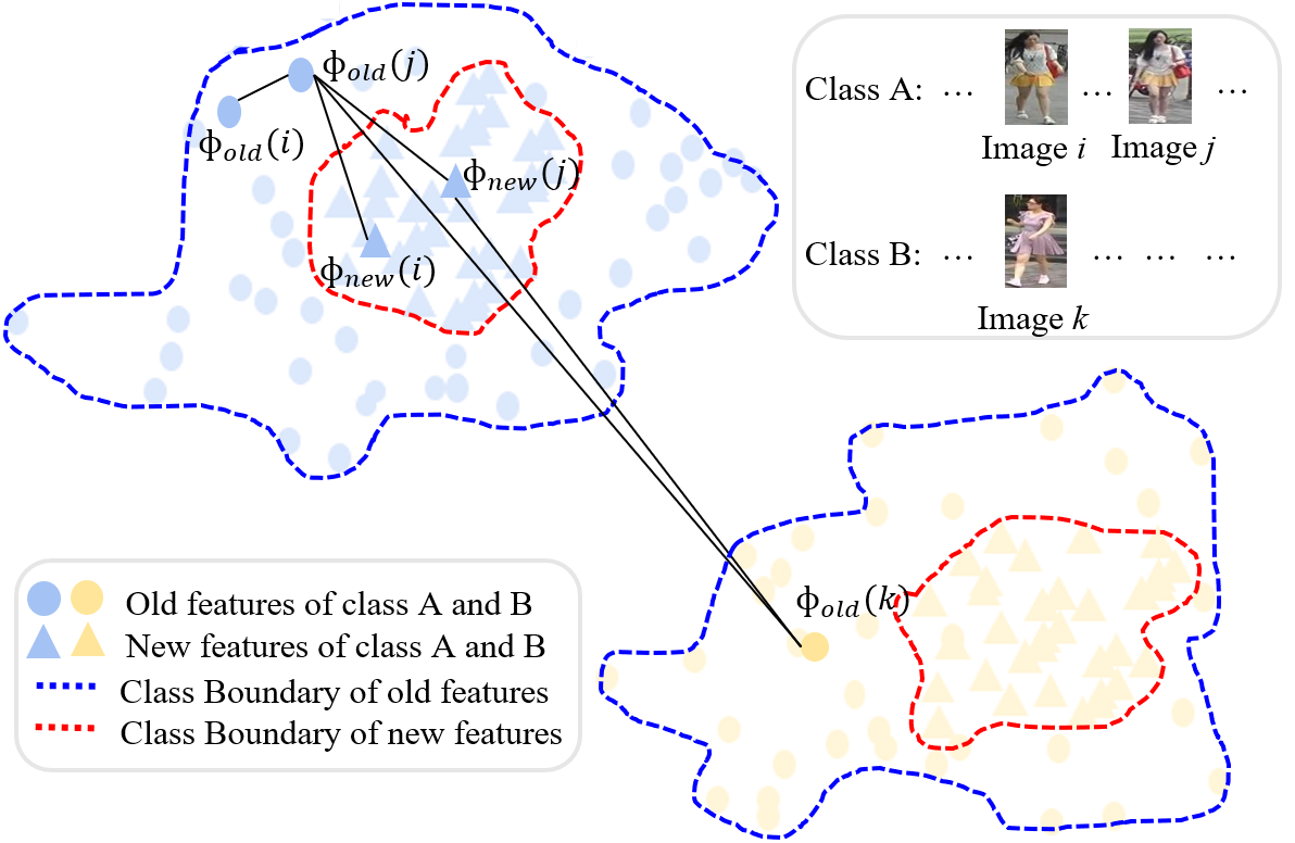
Figure 2: The distance relationship in the feature space. $\phi_{new}$ is compatiable with $\phi_{old}$, but pair $(i,j)$ and $(j,k)$ does not satify Inequality (1) and (2).

Shen et al. [22] give a strict criterion of backward-compatible compatibility in BCT.

$$d(\phi_{new}(i),\phi_{old}(j)) \geq d(\phi_{old}(i),\phi_{old}(j)),$$

$$\forall(i,j)\in\{(i,j):y_{i}\neq y_{j}\}.$$ (1)

$$d(\phi_{new}(i),\phi_{old}(j) \leq d(\phi_{old}(i),\phi_{old}(j)),$$

$$\forall(i,j)\in\{(i,j):y_{i}=y_{j}\}.$$ (2)

Such definition is the sufficient and unnecessary condition to achieve compatiblity, and it may impact $M(\phi_{new},\phi_{new})$. As shown in Figure 2, $\phi_{new}$ is compatible with $\phi_{old}$. However, we can find $d(\phi_{new}(j)$$,\phi_{old}(k))$$\leq$$d(\phi_{old}(j)$$,\phi_{old}(k))$, $d(\phi_{new}(i)$$,\phi_{old}(j))$$\geq$$d(\phi_{old}(i)$$,\phi_{old}(j))$, which do not satisfy Inequality (1) and (2). Constraining $\phi_{new}$ to satisfy them enlarge the class boundary of new features. Therefore, we come up with a new backward-compatible criterion:

$$d(\phi_{new}(i),\phi_{old}(j))<d(\phi_{new}(i),\phi_{old}(k)),$$

$$\forall(i,j,k)\in\{(i,j,k):y_{i}=y_{j}\neq y_{k}\}.$$ (3)

Inequality (3) is the minimal constraints to accomplish $M(\phi_{new},\phi_{old})$ $\geq$ $M(\phi_{old},\phi_{old})$. Given image $i$, the distance between anchor (termed as $\phi_{new}(i)$) and other fixed positives (termed as $\phi_{old}(j)$) is smaller than the distance between it and fixed negatives (termed as $\phi_{old}(k)$).

3.3 Neighborhood consensus compatible learning

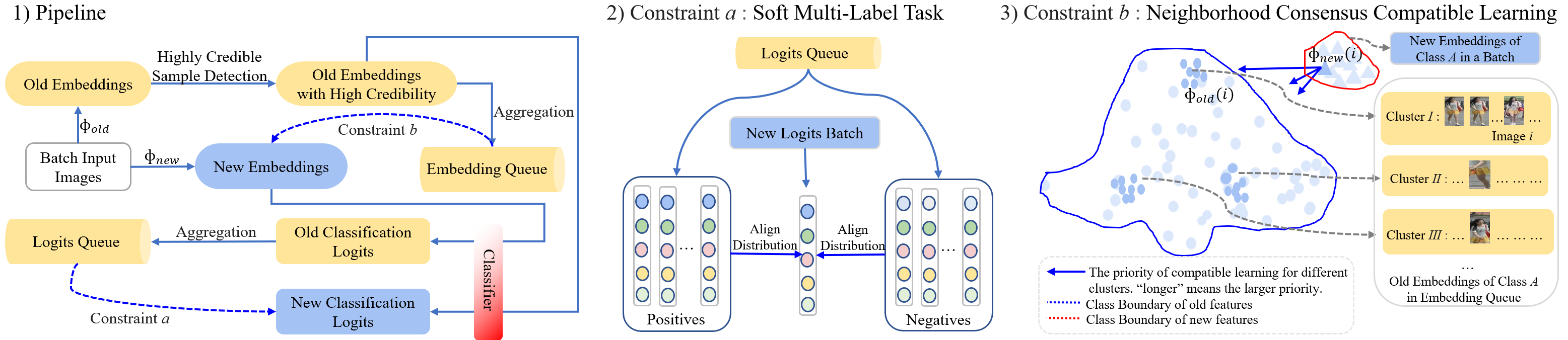
Figure 3: An illustration of our method NCCL. The left part shows the pipeline of using the old embeddings to regularize the new embeddings; The middle part shows that we use a soft multi-label task to align the discrimination distribution; The right part shows that we learn the compatible embeddings at cluster view.

To satisfy Inequality (3), a naive solution is to adopt the metric learning loss in an asymmetric way, e.g., triplet loss [3] and cross-entropy [22] . However, there are several limitations: 1) The potential manifold structure of the data can not be characterized by random sampling instances or classifiers [20]. 2) They are susceptible to those boundary points or outliers with the newly added data, making the training results unpredictable. 3) They treat all the old embeddings equally important, which can be overwhelmed by less informative pairs, resulting in inferior performance [24].

In this work, we propose a neighborhood consensus supervised contrastive learning method for backward-compatible learning. We proposed the neighborhood consensus weight to estimate the potential manifold structure. A FIFO memory queue is adapted to store the estimated clusters, updating by batches, termed as $\mathcal{B}$. Then we propose a contrastive loss to regularize the new embeddings with the old clusters. Define $A(i)\equiv\mathcal{B}\diagdown\{i\}$ and $P(i)\equiv\{p\in A(i):y_{p}=y_{i}\}$, our training objective on the embedding space is a weighted generalization of contrastive loss, given by

$$L_{1} =\sum_{i\in\mathcal{D}_{new}}\sum_{p\in P(i)}-w_{ip}\log s_{ip},$$ (4)

$$w_{ip} =\frac{1}{2}(\frac{\phi_{old}(i)\phi_{old}(p)}{||\phi_{old}(i)||||\phi_{old}(p)||}+1)\in[0,1],$$ (5)

$$s_{ip} =\frac{\exp(\phi_{new}(i)\phi_{old}(p)/\tau)}{\sum_{a\in A(i)}\exp(\phi_{new}(i)\phi_{old}(a)/\tau)}.$$ (6)

$w_{ip}$ estimates the sub-cluster structures by measuring the affinity relationship between anchors $i$ and fixed positives $p$. Ideally, each new anchor embedding should focus on the fixed positives from its corresponding old embedding cluster. However, the boundaries between local clusters may be blurred. Thus we adopt the soft weight to concentrate more on the positives, which are more informative. “More informative” means a higher probability to belong to a local cluster corresponding to the anchor. Given a positive image pair $(i,p)$ and view $i$ as the anchor, it is intuitive that the weight $w_{ip}$ of $\phi_{old}(p)$ rises in inverse proportion to the distance between $\phi_{old}(i)$ and $\phi_{old}(p)$. Specifically, $w_{ip}$ is calculated on the embeddings after L2 normalized by the cosine distance, regarded as the prior knowledge. We have tried other kernel-based similarity functions to calculate $w_{ip}$, e.g., t-distribution kernel $w_{ip}^{\prime}=\frac{(1+||\phi_{old}(i)-\phi_{old}(p)||^{2})^{-1}}{\sum_{a\in A(i)}(1+||\phi_{old}(i)-\phi_{old}(a)||^{2})^{-1}}$ , and gaussian kernel $w_{ip}^{\prime\prime}=\frac{\exp(\phi_{old}(i)\phi_{old}(p)/\tau)}{\sum_{a\in A(i)}\exp(\phi_{old}(i)\phi_{old}(a)/\tau)}$. We find that such $w_{ip}$ differs only slightly, and the mean average precision changes smaller than 0.5% (detailed in supplementary). Therefore, we calculate $w_{ip}$ by Equation (5) for simpilfily.

$s_{ip}$ represents the affinity score of positive $p$ contrasted with an anchor $i$, where $\tau$ is a temperature parameter that controls the sharpness of similarity distribution. Minimizing $L_{1}$ is equivalent to maximize the affinity scores between anchors and positives. The existence of weight forces the optimized gradient direction to be more biased towards those positive pairs that are geometrically closer. Therefore, the neighborhood consensus contrastive learning procedure on the embedding space actually ensures the alignment of the old and new embeddings at the granularity of local clusters.

3.4 Soft multi-label task on the discrimination space

As the embedding space represents the instance-level knowledge, the proposed neighborhood consensus supervised contrastive learning can be regarded as an intra-class alignment between old and new embeddings. While the discrimination space represents the class-level knowledge, which defines the probability distribution of each sample belonging to the underlying class centers on the simplex [36]. Intuitively, we can impose constraints on classifiers to achieve the class-level alignment and tightening.

With the new classifier, we construct a pseudo-multi-label task from a different perspective than semantic-level label learning. Specifically, given image $i$, its positive image set $P$ and negative image set $N$, we compare the discrimination vector $\varphi_{new}(\phi_{new}(i))$ with discrimination vector set $\{\varphi_{new}(\phi_{old}(p)),p\in P\}$ and $\{\varphi_{new}(\phi_{old}(n)),n\in N\}$. Intuitively, $\varphi_{new}(\phi_{new}(i))$ should be similar to any positive discrimination vector $\varphi_{new}(\phi_{old}(p))$ and dissimilar to any negative discrimination vector $\varphi_{new}(\phi_{old}(n))$. Thus, the positive/negative discrimination vectors can be regarded as pseudo-multi-labels as a supplement to ground truth. As the ground truth may only reflect a single facet of the complete knowledge encapsulated in real-world data [30], such label is an auxiliary to mine richer knowledge, resulting in the new embeddings with better performance. Here we imitate the contrastive procedure in the embedding space for harmonization. A FIFO memory queue is also utilized to store the positive/negative discrimination vector. We give the dual soft contrastive loss on the discrimination space below,

$$L_{2}=\sum_{i\in\mathcal{D}_{new}}\sum_{p\in P(i)}-w_{ip}\log\tilde{s}_{ip},$$ (7)

$$\tilde{s}_{ip}=\frac{\exp(\varphi_{new}(\phi_{new}(i))\varphi_{new}(\phi_{old}(p))/\tau)}{\sum_{a\in A(i)}\exp(\varphi_{new}(\phi_{new}(i))\varphi_{new}(\phi_{old}(x_{a}))/\tau)}.$$ (8)

where the weight $w_{ip}$ is the same as in Equation (5).

Discussion. Regarding how to constrain the new and old discrimination vectors, there are the following options: 1) Constrain the new and old discrimination vectors to be consistent with their one-hot semantic label (e.g., using the cross-entropy). Such vectors with the same ID tend to fall in the same hyperplane block. However, it is difficult to converge to an ideal one-hot form, especially in a large amount of IDs scenario. Thus, the distance between new and old embeddings with the same ID may be large, which means backward compatibility is not ensured. 2) Constrain the new discrimination vectors to be consistent with their corresponding old ones (e.g., using the KL divergence). Such vectors corresponding to the same image tend to be consistent. However, the divergence or variance of the discrimination distribution for each class may be larger, impacting the performance of the new model. 3) To achieve compatibility with the new embeddings more compact, we jump out of the constrain of pair-based methods. We use the discrimination vectors of other samples with the same ID in the neighborhoods to constrain each other. As a result, such new vectors tend to be consistent at a cluster level, as a new vector and its neighbor are regularized by the same old discrimination vectors.

3.5 Highly credible sample detection

Due to the variations of object morphology, illumination, and camera view in the real-world data, the intra-class variance of old embeddings can be huge [2]. Poor old embeddings are often located in the fuzzy region between classes. Compatible learning with such outlier samples would affect the retrieval accuracy of the new model.

Here, we introduce entropy to measure the uncertainty of sample classification. With greater entropy, the classification vectors tend to have smaller credibility. One straightforward method to construct the classification vectors is to use the old classifier. However, the old classifier can not handle newly added classes. Besides, it is not available when a third party deploys the old model, as shown in Figure 1. Therefore, we construct the pseudo classification vectors $\tilde{p}(x)$ by calculating the similarity score of each sample belonging to old class centers. Specifically, suppose the $\hat{\mu}_{k}=\frac{1}{|\{i:y_{i}=k\}|}\sum_{y_{i}=k}\phi_{old}(i)$ is the $k$-th ($1\leq k\leq K_{new}$) old class center. Here we test the reliability of $\hat{\mu}_{k}$ through a simple experiment: for the model ResNet18 trained by 50% data on Market1501, the mAP is only 63.26%. However, the discrimination accuracy of using the nearest geometry center is 96.35% and 99.17% for the test set and training set, respectively, proving its effectiveness. Then we utilize multiple Gaussian kernel functions to obtain the similarity score between samples and centers,

$$\tilde{p}(i)_{k}=\frac{\exp(-\frac{||\phi_{old}(i)-\hat{\mu}_{k}||^{2}}{\hat{\sigma}_{k}})}{\sum_{j=1}^{K_{new}}\exp(-\frac{||\phi_{old}(i)-\hat{\mu}_{j}||^{2}}{\hat{\sigma}_{j}})}.$$ (9)

Where $\hat{\sigma}_{k}$ represents the variance of $k$-th distance set $\{||\phi_{old}(i)-\hat{\mu}_{k}||^{2}:y_{i}=k\}$. Then the uncertainty of $i$-th sample is the entropy of $\tilde{p}(i)$, namely $\mathcal{H}(i)=\sum_{k=1}^{K_{new}}-\tilde{p}(i)_{k}\log\tilde{p}(i)_{k}$. Since $\log K_{new}$ is the maximum value of $\mathcal{H}$, the uncertainty threshold boundary is set as $\hat{U}$ which is related to $\log K_{new}$. Then we remove those samples with entropy larger than $\hat{U}$, and they do not participate in the soft supervised contrastive learning procedure.

Overall loss function. Combining with classification loss $Loss_{new}$ on the new model trained independently, we give the final objective below,

$$L_{total}=L_{new}+\alpha L_{1}+\beta L_{2}.$$ (10)

Where the $\alpha$ and $\beta$ are two hyperparameters to control the relative importance of embedding space learning and discrimination space learning, respectively.

Table 1: Performance comparison on Market1501, MSMT17 and VeRi-776 datasets.

	Market1501				MSMT17				VeRi-776
Methods	Self-Test		Cross-Test		Self-Test		Cross-Test		Self-Test		Cross-Test
	R1	mAP	R1	mAP	R1	mAP	R1	mAP	R1	mAP	R1	mAP
Ori-Old(R18)	82.96	63.26	-	-	57.02	29.24	-	-	89.35	56.91	-	-
$L_{2}$ regression	91.66	78.69	3.03	2.27	67.3	39.57	0.51	0.26	91.13	63.75	4.23	2.97
BCT	91.69	77.47	84.74	66.86	67.91	39.11	58.18	30.44	92.02	64	80.86	56.41
Asymmetric	91.98	81.08	85.45	68.4	71.95	45.29	53.90	28.15	91.26	66.59	81.01	56.28
NCCL(Ours)	92.87	81.90	85.51	69.15	73.43	46.00	59.64	30.92	92.62	70.15	81.37	58.82
Ori-New(R18)	92.37	80.84	22.71	13.81	70.52	42.86	10.06	4.11	92.26	67.21	19.70	10.00
Ori-Old(R50)	87.23	70.48	-	-	64.29	36.45	-	-	91.90	62.91	-	-
$L_{2}$ regression	93.97	84.31	47.30	28.97	72.43	47.16	30.91	13.22	93.15	70.61	47.50	25.64
BCT	93.35	82.51	90.50	75.21	71.25	45.07	68.77	40.45	92.02	67.49	88.44	64.89
Asymmetric	94.39	86.42	90.32	77.34	75.37	51.44	70.43	41.68	92.27	70.19	89.70	63.41
NCCL(Ours)	94.80	87.24	91.60	77.69	77.55	52.97	71.45	42.87	94.4	75.42	89.70	66.74
Ori-New(R50)	94.30	85.10	81.98	60.78	73.58	48.42	52.46	26.47	93.69	70.70	65.48	37.90

4 Experiments

We evaluate our proposed method on two widely-used person ReID datasets, i.e., Market-1501 [39], MSMT17 [28], and one vehicle ReID dataset VeRi-776 [27]. We first implement several baselines, and then test the potential of our method by applying it to the case of multi-factor changes, including model changes and loss changes. We also conduct a multi-model test to evaluate the sequential compatibility. Besides, we adopt the large-scale ImageNet [8] and Place365 [43] datasets to demonstrate the scalability of our method.

4.1 Datasets and evaluation metrics

Market1501 consists of 32,668 annotated images of 1,501 identities shot from 6 cameras in total. MSMT17 is a large-scale ReID dataset consisting of 126,441 bounding boxes of 4,101 identities taken by 15 cameras. VeRi-776 contains over 50,000 images of 776 vehicles captured by 20 cameras.ImageNet contains more than 1.2 million images with 1,000 classes. Place365 has about 1.8 million images with 365 classes. For ImageNet and Place365, we conduct the retrieval process on the validation sets of these two datasets, i.e., each image will be taken as a query image, and other images will be regarded as gallery images.

Mean average precision (mAP) and top-$k$ accuracy are adopted to evaluate the performances of retrieval. $M(\phi_{new},\phi_{new})$ (termed as “self-test”) and $M(\phi_{new},\phi_{old})$ (termed as “cross-test”) are used to evaluate the performances of backward-compatible representation.

4.2 Implementation details

The implementations of all compared methods and our NCCL are based on the FastReID [13]. The default configuration in “SBS” is adopted for the model using “CircleSoftmax” and “ArcSoftmax”. And the default configuration in “bagtricks” is adopted for the model using “Softmax” with slight changes: size_train/size_test is set to 384x128 to be consistent with “SBS”. The size of $\mathcal{B}$ is 2048 and $\tau$ is 1.0. We set $\alpha$ and $\beta$ around 0.01 so that $L_{1}$ loss and $L_{2}$ loss are on the same order of magnitude as $L_{new}$ loss. $\hat{U}$ is set to $\frac{\log K_{new}}{2}$ as the credible sample selection threshold. More detail is shown in the suplementary.

4.3 Baseline comparisons

In this section, we conduct several baseline approaches with backbone ResNet-18 and ResNet-50. With the same model architectures and loss functions, we set the old training data of 50% IDs subset and the new training data of 100% IDs complete set. The results are shown in Table 1.

No regularization between $\phi_{new}$ and $\phi_{old}$. We denote the new model trained without any regularization as $\phi_{new*}$. A simple case directly performs a cross-test between $\phi_{new*}$ and $\phi_{old}$. As is shown in Table 1, backward compatibility is achieved at a certain degree. However, the cross-test accuracy fluctuates dramatically with the change of data set and network architecture, which is insufficient to satisfy our backward-compatibility criterion. Subsequent experimental results will further confirm this opinion.

$L_{2}$-regression between $\phi_{new}$ and $\phi_{old}$ output embeddings. An intuitive idea to achieve backward-compatibility is using $L_{2}$ loss to minimize the output embeddings’ euclidean distance between $\phi_{new}$ and $\phi_{old}$, which was discussed in [22]. Such a simple baseline could not meet the requirement of backward-compatibility learning. The possible reason for $L_{2}$ loss failure is that $L_{2}$ loss is too local and restrictive. It only focuses on decreasing the distance between feature pairs from the same image, ignoring the distance restriction between negative pairs.

Asymmetric. It works better on small datasets than on large-scale datasets, probably owing to its inadequacy in utilizing the intrinsic data structure. For instance, Asymmetric’s cross-test outperforms the old model’s self-test on Market1501, but not on VeRi-776, as is shown in Table 1.

BCT. As is shown in Table 1, BCT underperforms $\phi_{new*}$ in all self-test cases. The most likely reason is that BCT use synthesized classifier weights or knowledge distillation to deal with the newly added data. Synthesized classifier weights for the newly added data are susceptible to those boundary points or outliers, making the training results unpredictable. Knowledge distillation assumes that the teacher model (old model) outperforms the student model (new model), which is not true in the application scenario of backward-compatible representation. As a result, it impairs the performance of the new model.

NCCL(Ours) with better self-test accuracy. As the effective utilization of the intrinsic structure, NCCL outperforms all compared methods. Besides, it significantly outperforms $\phi_{new*}$ in all self-test cases. Although all the data are accessible from the new model, the old model provides external knowledge due to its different architectures, initializations, training details, etc [37]. The key to better self-test accuracy is in extracting useful knowledge from the old model and eliminating the impact of outliers in the old embeddings. BCT does not take it into account but distills at the instance level and constrains the distributions of the new embeddings to be consistent with the old. We use entropy to measure the uncertainty of sample classification, so most outliers are filtered. Besides, we take a contrastive loss with multiple positives and negatives at the sub-class level. Thus the effects of the outliers are diminished as multiple old embeddings serve as “mean teachers”, similar to [31]. Such loss constrains the distance relationship between the new and old embeddings to be consistent.

4.4 Changes in network architectures and loss functions

Here we study whether each method can be stably applied to various model changes and loss function changes.

Table 2: Performance comparison between different models on Market1501. The old model uses ResNet-18 with 50% training data. “mAP1” and “mAP2” represent the mean average precision of self-test and cross-test, respectively.

	ResNet18-Ibn		ResNet50		ResNeSt50
Methods	mAP1	mAP2	mAP1	mAP2	mAP1	mAP2
Ori-Old	63.26	-	63.36	-	63.26	-
$L_{2}$ regression	80.05	1.19	84.54	0.56	83.03	0.59
BCT	78.92	66.70	82.03	68.65	86.64	68.76
Asymmetric	82.23	68.54	83.96	67.31	87.81	68.76
NCCL(Ours)	83.23	69.12	85.91	69.26	88.31	68.94
Ori-New	81.59	5.12	84.88	0.20	88.21	0.20

Model Changes. We first test the new model on ResNet18-Ibn, ResNet-50 and ResNeSt-50 [35] instead of the old model ResNet-18 under the same loss function. ResNet18-Ibn only changes the normalization method of the backbone from batch normalization to instance batch normalization [19], and it keeps the structure consistent. It can be seen as a slight modification to the old model. ResNet-50 is composed of the same components with different capacities compared to ResNet-18, which can be regarded as a middle modification to the old model. ResNeSt-50 introduces the split attention module into ResNet50, which makes it the most different from ResNet18. Note that the dimension of the feature vector in ResNet-50 and ResNeSt-50 is 2048. We will not directly feed the old feature with dimension 512 to $\phi_{new}$ but use the zero-padding method to expand it to 2048-dimension.

As shown in Table 2, the comparison between independently trained new models and old models is an epic failure. BCT, Asymmetric, and our proposed method have learned compatible representation. Besides, our approach remains the the-state-of-art and is more robust to model changes.

Table 3: Performance comparison between different losses on Market1501. The old model uses ResNet-18 with 50% training data. “mAP1” and “mAP2” represent the mean average precision of self-test and cross-test, respectively.

	CircleSoftmax		ArcSoftmax		Softmax+Triplet
Methods	mAP1	mAP2	mAP1	mAP2	mAP1	mAP2
Ori-Old	63.26	-	63.36	-	63.26	-
$L_{2}$ regression	62.67	3.29	54.03	0.85	81.27	23.53
BCT	67.63	53.20	63.49	39.96	79.62	67.43
Asymmetric	67.27	28.77	56.71	5.09	81.75	68.07
NCCL(Ours)	79.62	49.28	71.06	31.38	82.36	69.15
Ori-New	78.96	3.69	67.31	0.93	81.55	14.20

Loss Changes. Then we change the “Softmax” based loss function $L_{new}$ to “ArcSoftmax” [9], “CircleSoftmax” [23] and “Softmax + Triplet” in the new model. The first two are both used in the classification head, and the last “Triplet” is used in the embedding head.

As shown in Table 3, the performances of various methods are consistent with the baseline under the change of embedding loss. In contrast, all methods have a significant decline in self-test and cross-test under classification loss changes. The possible reason is that classification loss in the new models determines the class structure, while the embedding loss tightens the sample’s representation. Among these methods, Asymmetric fails in both self-test and cross-test. BCT achieves slightly better performance in cross-test but significantly reduces new models’ performance, making it unnecessary to deploy new models. Our method can improve the performance of the new model stably while ensuring the performance of the cross-test.

4.5 No overlap between $\mathcal{D}_{old}$ and $\mathcal{D}_{new}$

When the old model is from a third party, all of its information, including the classifier and training sets, are unavailable, except for the embedding backbone. In the previous experiments, we always assume that the $\mathcal{D}_{new}$ is a superset of $\mathcal{D}_{old}$. Here we investigate whether no overlap between them could sharply affect the compatibility performance of each method. The old model is trained with the randomly sampled 25% IDs subset of training data in the Market1501 dataset, and the new model is trained with the other 75% IDs subset. We show the results in Table 4.

Compared with baseline, the accuracy of all evaluated methods has dropped, except for NCCL. The performance degradation of BCT is the most severe because it can only use synthesized classifier weights or knowledge utilization in this case. Both of them can be regarded as a kind of knowledge distillation at the instant level. As the old model is not good enough, BCT is difficult to extract useful knowledge and eliminate the impact of outliers in the old embeddings. Our model has carefully considered such cases. Thus we achieve the same effect as the baseline in this case.

Table 4: Performance comparison of no overlap between $\mathcal{D}_{old}$ (25% IDs) and $\mathcal{D}_{new}$ (75% IDs) on Market1501.

	Self-Test			Cross-Test
Methods	R1	R5	mAP	R1	R5	mAP
Ori-Old	70.13	86.07	46.42	-	-	-
$L_{2}$ regression	90.29	96.32	76.24	15.86	35.33	9.41
BCT	86.73	94.86	69.60	62.29	83.49	41.63
Asymmetric	91.03	96.67	78.91	74.55	90.23	53.07
NCCL(Ours)	92.22	97.09	80.88	77.73	90.94	55.91
Ori-New	90.17	96.32	77.52	6.00	16.60	3.92

4.6 Multi-model and sequential compatibility

Here we investigate the sequential compatibility case of multi-model. There are three models: $\phi_{1}$, $\phi_{2}$ and $\phi_{3}$. $\phi_{1}$ is trained with the randomly sampled 25% IDs subset of training data in the Market1501 dataset. $\phi_{2}$ is trained with a 50% subset. And $\phi_{3}$ is trained with the full dataset. We constrain $\phi_{2}$ to be compatible with $\phi_{1}$ and $\phi_{3}$ to be compatible with $\phi_{2}$. Thus, $\phi_{3}$ has no direct influence on $\phi_{1}$. The results of the sequential compatibility test are shown in Table 5.

We observe that, by training with NCCL, the last model $\phi_{3}$ is transitively compatible with $\phi_{1}$ even though $\phi_{1}$ is not directly involved in training $\phi_{3}$. It shows that transitive compatibility between multiple models is achievable through our method, enabling a sequential update of models. It is worth mentioning that our approach still has significant advantages over other methods in cross-model comparison $\phi_{3}2\phi_{1}$.

Table 5: Performance comparison in sequential multi-modal experiment on Market1501. We train three models $\phi_{1}$ (ResNet18+25% IDs), $\phi_{2}$ (ResNet18+50% IDs) and $\phi_{3}$ (ResNet18+100% IDs).

	Market1501 (mAP)
Methods	$(\phi_{1},\phi_{1})$	$(\phi_{2},\phi_{1})$	$(\phi_{2},\phi_{2})$	$(\phi_{3},\phi_{2})$	$(\phi_{3},\phi_{3})$	$(\phi_{3},\phi_{1})$
Ori	46.42	7.49	63.30	14.15	80.85	5.62
$L_{2}$ regression	-	24.01	61.87	16.15	78.39	1.47
BCT	-	45.78	60.29	65.45	77.07	45.20
Asymmetric	-	45.68	62.88	67.51	81.28	48.85
NCCL(Ours)	-	45.89	64.27	69.76	82.28	52.76

4.7 Test on other two large-scale image datasets

As the need for backward-compatible learning stems from the fact that the gallery is too large to re-extract new embeddings, we also utilize large-scale ImageNet and Place365 datasets for training and evaluating each method. The results are shown in Table 6. On large-scale datasets, the accuracy of Asymmetric drops significantly. NCCL achieves better performance than baseline. Asymmetric is too local and restrictive to capture the intrinsic structure in the large datasets, while our method has a solid ability to obtain the intrinsic structure.

Table 6: Performance comparison on two large-scale datasets, ImageNet and Place365. The new model uses ResNet-18 with 50% Data, while the new model uses ResNet-50 with 100% Data.

	Place365				ImageNet
Methods	Self-Test		Cross-Test		Self-Test		Cross-Test
	Top-1	Top-5	Top-1	Top-5	Top-1	Top-5	Top-1	Top-5
Ori-Old	27.0	55.9	-	-	39.5	60.0	-	-
BCT	32.7	62.2	27.6	57.6	41.9	65.3	42.2	65.5
Asymmetric	31.2	60.9	28.6	58.1	41.8	65.1	42.9	63.3
NCCL(Ours)	35.1	64.1	28.7	58.1	62.5	81.6	46.1	68.2
Ori-New	35.1	64.0	-	-	62.5	81.5	-	-

4.8 Discussion

Generally, three motivations drive us to deploy a new model: 1) growth in training data, 2) better model architecture, and 3) better loss functions. We have conducted detailed experiments on these three aspects. BCT can deal with the data growth and model architecture changes when the old and new training data have common classes. Asymmetric can handle data growth and model architecture changes well on small datasets, even better than BCT, but it is too local to work on large datasets reliably. Our method is state-of-the-art under the changes of training data and model architectures. It achieves better cross-test performance and gives better performance than the new model trained independently.

For loss functions, the change of embedding loss usually does not affect backward-compatible learning. In contrast, the change of classification loss will lead to both BCT failure and Asymmetric failure, which means that the cross-test performance drops sharply or the new model’s performance is significantly damaged. However, our method can still improve the performance of the new model under the variation of classification loss. At the same time, the backward-compatible version is obtained.

4.9 Ablation study

We test the effect of different modules in NCCL. As is shown in Table 7, we can observe that adaptive neighborhood consensus helps to strengthen both self-test and cross-test performance significantly. The soft pseudo-multi-label learning also improves performance steadily but not as significantly as the neighborhood consensus module. Besides, the proposed highly credible sample detection procedure does not bring significant performance up-gradation in all cases, which depends on the quality of the old model.

Table 7: Ablation study on Market1501. The new model is trained with 100 % Data using ResNet-18.

	Self-Test			Cross-Test
Methods	R1	R5	mAP	R1	R5	mAP
Ori-Old(R18+50 %Data)	82.96	92.32	63.26	-	-	-
NCCL w/o neighborhood consensus	91.75	97.14	78.71	85.45	93.48	67.90
NCCL w/o pseudo-multi-label learning	91.98	97.48	80.08	85.51	94.83	68.40
NCCL w/o sample selection	92.58	97.30	80.18	85.05	95.07	68.72
NCCL	92.87	97.58	81.9	86.05	95.34	69.15
Ori-Old(R18+25 %Data)	70.13	86.07	46.42	-	-	-
NCCL w/o neighborhood consensus	91.81	97.09	79.40	76.63	91.57	55.60
NCCL w/o pseudo-multi-label learning	91.92	97.06	80.57	78.06	91.69	56.53
NCCL w/o sample selection	91.86	96.97	80.13	77.35	91.51	55.71
NCCL	92.64	97.24	81.41	78.06	91.98	57.44

5 Conclusion

This paper proposes a neighborhood consensus contrastive learning framework with credible sample selection for feature compatible learning. We validate the effectiveness of our method by conducting thorough experiments in various reality scenarios using three ReID datasets and two large-scale retrieval datasets. Our method achieves the state-of-the-art performances and shows convincing robustness in different case studies.

References

- [1] Song Bai, Peng Tang, Philip HS Torr, and Longin Jan Latecki. Re-ranking via metric fusion for object retrieval and person re-identification. In Proceedings of the IEEE Conference on Computer Vision and Pattern Recognition, pages 740–749, 2019.
- [2] Yan Bai, Yihang Lou, Feng Gao, Shiqi Wang, Yuwei Wu, and Ling-Yu Duan. Group-sensitive triplet embedding for vehicle reidentification. IEEE Transactions on Multimedia, 20(9):2385–2399, 2018.
- [3] Mateusz Budnik and Yannis Avrithis. Asymmetric metric learning for knowledge transfer. arXiv preprint arXiv:2006.16331, 2020.
- [4] Mathilde Caron, Ishan Misra, Julien Mairal, Priya Goyal, Piotr Bojanowski, and Armand Joulin. Unsupervised learning of visual features by contrasting cluster assignments. In Thirty-fourth Conference on Neural Information Processing Systems, 2020.
- [5] Dapeng Chen, Dan Xu, Hongsheng Li, Nicu Sebe, and Xiaogang Wang. Group consistent similarity learning via deep crf for person re-identification. In Proceedings of the IEEE conference on computer vision and pattern recognition, pages 8649–8658, 2018.
- [6] Ting Chen, Simon Kornblith, Kevin Swersky, Mohammad Norouzi, and Geoffrey Hinton. Big self-supervised models are strong semi-supervised learners. arXiv preprint arXiv:2006.10029, 2020.
- [7] Xinlei Chen, Haoqi Fan, Ross Girshick, and Kaiming He. Improved baselines with momentum contrastive learning. arXiv preprint arXiv:2003.04297, 2020.
- [8] Jia Deng, Wei Dong, Richard Socher, Li-Jia Li, Kai Li, and Li Fei-Fei. Imagenet: A large-scale hierarchical image database. 2009 IEEE conference on computer vision and pattern recognition, pages 248–255, 2009.
- [9] Jiankang Deng, Jia Guo, Niannan Xue, and Stefanos Zafeiriou. Arcface: Additive angular margin loss for deep face recognition. Proceedings of the IEEE Conference on Computer Vision and Pattern Recognition, pages 4690–4699, 2019.
- [10] Yang Fu, Xiaoyang Wang, Yunchao Wei, and Thomas Huang. Sta: Spatial-temporal attention for large-scale video-based person re-identification. In Proceedings of the AAAI conference on artificial intelligence, 33(1):8287–8294, 2019.
- [11] Jean-Bastien Grill, Florian Strub, Florent Altché, Corentin Tallec, Pierre H Richemond, Elena Buchatskaya, Carl Doersch, Bernardo Avila Pires, Zhaohan Daniel Guo, Mohammad Gheshlaghi Azar, et al. Bootstrap your own latent: A new approach to self-supervised learning. arXiv preprint arXiv:2006.07733, 2020.
- [12] Raia Hadsell, Sumit Chopra, and Yann LeCun. Dimensionality reduction by learning an invariant mapping. In 2006 IEEE Computer Society Conference on Computer Vision and Pattern Recognition (CVPR’06), 2006.
- [13] Lingxiao He, Xingyu Liao, Wu Liu, Xinchen Liu, Peng Cheng, and Tao Mei. Fastreid: A pytorch toolbox for general instance re-identification. arXiv preprint arXiv:2006.02631, 6(7):8, 2020.
- [14] Ruibing Hou, Bingpeng Ma, Hong Chang, Xinqian Gu, Shiguang Shan, and Xilin Chen. Vrstc: Occlusion-free video person re-identification. In Proceedings of the IEEE Conference on Computer Vision and Pattern Recognition, pages 7183–7192, 2019.
- [15] Sultan Daud Khan and Habib Ullah. A survey of advances in vision-based vehicle re-identification. Computer Vision and Image Understanding, 182:50–63, 2019.
- [16] Jianing Li, Jingdong Wang, Qi Tian, Wen Gao, and Shiliang Zhang. Global-local temporal representations for video person re-identification. In Proceedings of the IEEE International Conference on Computer Vision, pages 3958–3967, 2019.
- [17] Junnan Li, Pan Zhou, Caiming Xiong, Richard Socher, and Steven CH Hoi. Prototypical contrastive learning of unsupervised representations. arXiv preprint arXiv:2005.04966, 2020.
- [18] Aaron van den Oord, Yazhe Li, and Oriol Vinyals. Representation learning with contrastive predictive coding. arXiv preprint arXiv:1807.03748, 2018.
- [19] Xingang Pan, Ping Luo, Jianping Shi, and Xiaoou Tang. Two at once: Enhancing learning and generalization capacities via ibn-net. Proceedings of the European Conference on Computer Vision, pages 464–479, 2018.
- [20] Qi Qian, Lei Shang, Baigui Sun, Juhua Hu, Hao Li, and Rong Jin. Softtriple loss: Deep metric learning without triplet sampling. Proceedings of the IEEE International Conference on Computer Vision, pages 6450–6458, 2019.
- [21] Filip Radenović, Ahmet Iscen, Giorgos Tolias, Yannis Avrithis, and Ondřej Chum. Revisiting oxford and paris: Large-scale image retrieval benchmarking. In Proceedings of the IEEE Conference on Computer Vision and Pattern Recognition, pages 5706–5715, 2018.
- [22] Yantao Shen, Yuanjun Xiong, Wei Xia, and Stefano Soatto. Towards backward-compatible representation learning. In Proceedings of the IEEE Conference on Computer Vision and Pattern Recognition, pages 6368–6377, 2020.
- [23] Yifan Sun, Changmao Cheng, Yuhan Zhang, Chi Zhang, Liang Zheng, Zhongdao Wang, and Yichen Wei. Circle loss: A unified perspective of pair similarity optimization. Proceedings of the IEEE Conference on Computer Vision and Pattern Recognition, pages 6398–6407, 2020.
- [24] Xun Wang, Xintong Han, Weilin Huang, Dengke Dong, and Matthew R Scott. Multi-similarity loss with general pair weighting for deep metric learning. In Proceedings of the IEEE/CVF Conference on Computer Vision and Pattern Recognition, pages 5022–5030, 2019.
- [25] Xudong Wang, Ziwei Liu, and Stella X Yu. Unsupervised feature learning by cross-level discrimination between instances and groups. arXiv preprint arXiv:2008.03813, 2020.
- [26] Yicheng Wang, Zhenzhong Chen, Feng Wu, and Gang Wang. Person re-identification with cascaded pairwise convolutions. In Proceedings of the IEEE Conference on Computer Vision and Pattern Recognition, pages 1470–1478, 2018.
- [27] Zhongdao Wang, Luming Tang, Xihui Liu, Zhuliang Yao, Shuai Yi, Jing Shao, Junjie Yan, Shengjin Wang, Hongsheng Li, and Xiaogang Wang. Orientation invariant feature embedding and spatial temporal regularization for vehicle re-identification. Proceedings of the IEEE International Conference on Computer Vision, pages 379–387, 2017.
- [28] Longhui Wei, Shiliang Zhang, Wen Gao, and Qi Tian. Person transfer gan to bridge domain gap for person re-identification. Proceedings of the IEEE conference on computer vision and pattern recognition, pages 79–88, 2018.
- [29] Nicolai Wojke and Alex Bewley. Deep cosine metric learning for person re-identification. In 2018 IEEE winter conference on applications of computer vision, pages 748–756, 2018.
- [30] Guodong Xu, Ziwei Liu, Xiaoxiao Li, and Chen Change Loy. Knowledge distillation meets self-supervision. In European Conference on Computer Vision, pages 588–604. Springer, 2020.
- [31] Y. Xu, X. Qiu, L. Zhou, and X. Huang. Improving bert fine-tuning via self-ensemble and self-distillation. 2020.
- [32] Hantao Yao, Shiliang Zhang, Richang Hong, Yongdong Zhang, Changsheng Xu, and Qi Tian. Deep representation learning with part loss for person re-identification. IEEE Transactions on Image Processing, 28(6):2860–2871, 2019.
- [33] Mang Ye, Chao Liang, Zheng Wang, Qingming Leng, and Jun Chen. Ranking optimization for person re-identification via similarity and dissimilarity. In Proceedings of the 23rd ACM international conference on Multimedia, pages 1239–1242, 2015.
- [34] Mang Ye, Jianbing Shen, Gaojie Lin, Tao Xiang, Ling Shao, and Steven CH Hoi. Deep learning for person re-identification: A survey and outlook. IEEE Transactions on Pattern Analysis and Machine Intelligence, 2021.
- [35] Hang Zhang, Chongruo Wu, Zhongyue Zhang, Yi Zhu, Zhi Zhang, Haibin Lin, Yue Sun, Tong He, Jonas Mueller, R Manmatha, et al. Resnest: Split-attention networks. arXiv preprint arXiv:2004.08955, 2020.
- [36] Yifan Zhang, Bryan Hooi, Dapeng Hu, Jian Liang, and Jiashi Feng. Unleashing the power of contrastive self-supervised visual models via contrast-regularized fine-tuning. arXiv preprint arXiv:2102.06605, 2021.
- [37] Ying Zhang, Tao Xiang, Timothy M Hospedales, and Huchuan Lu. Deep mutual learning. In Proceedings of the IEEE Conference on Computer Vision and Pattern Recognition, pages 4320–4328, 2018.
- [38] Liming Zhao, Xi Li, Yueting Zhuang, and Jingdong Wang. Deeply-learned part-aligned representations for person re-identification. In Proceedings of the IEEE international conference on computer vision, pages 3219–3228, 2017.
- [39] Liang Zheng, Liyue Shen, Lu Tian, Shengjin Wang, Jingdong Wang, and Qi Tian. Scalable person re-identification: A benchmark. Proceedings of the IEEE international conference on computer vision, pages 1116–1124, 2015.
- [40] Jincheng Zhong, Ximei Wang, Zhi Kou, Jianmin Wang, and Mingsheng Long. Bi-tuning of pre-trained representations. arXiv preprint arXiv:2011.06182, 2020.
- [41] Jincheng Zhong, Ximei Wang, Zhi Kou, Jianmin Wang, and Mingsheng Long. Bi-tuning of pre-trained representations. arXiv preprint arXiv:2011.06182, 2020.
- [42] Zhun Zhong, Liang Zheng, Zhiming Luo, Shaozi Li, and Yi Yang. Invariance matters: Exemplar memory for domain adaptive person re-identification. In Proceedings of the IEEE Conference on Computer Vision and Pattern Recognition, pages 598–607, 2019.
- [43] Bolei Zhou, Agata Lapedriza, Aditya Khosla, Aude Oliva, and Antonio Torralba. Places: A 10 million image database for scene recognition. IEEE transactions on pattern analysis and machine intelligence, 40(6):1452–1464, 2017.
- [44] Kaiyang Zhou, Yongxin Yang, Andrea Cavallaro, and Tao Xiang. Omni-scale feature learning for person re-identification. In Proceedings of the IEEE International Conference on Computer Vision, pages 3702–3712, 2019.