Two Basic Queueing Models of Service Platforms in Digital Sharing Economy

Abstract

This paper describes two basic queueing models of service platforms in digital sharing economy by means of two different policies of platform matching information. We show that the two queueing models of service platforms can be expressed as the level-independent quasi birth-and-death (QBD) processes. Using the proposed QBD processes, we provide a detailed analysis for the two queueing models of service platforms, including the system stability, the average stationary numbers of seekers and of idle owners, the expected sojourn time of an arriving seeker, and the expected profits for both the service platform and each owner. Finally, numerical examples are employed to verify our theoretical results, and demonstrate how the performance measures of service platforms are influenced by some key system parameters. We believe that the methodology and results developed in this paper not only can be applied to develop a broad class of queuing models of service platforms, but also will open a series of promising innovative research on performance evaluation, optimal control and queueing-game of service platforms and digital sharing economy.

Keywords: Service platform, sharing economy; queueing model; QBD process; matrix-geometric solution; RG-factorization.

1 Introduction

In the past few years, with great advances of wireless, mobile, Internet and digital technologies, we have witnessed rapid rise of digital, platform and sharing economies, which have become a class of increasingly important economic modes in the current world. Many famous companies of service platforms continue to emerge and develop rapidly. Important examples include taxi-style transportation: Uber, Lyft, Didi; rental housing: AirBnB, HomeAway; restaurant food delivery: Caviar, DoorDash; consumer goods delivery: UberRush, Go-Mart; and so forth. For more details of sharing economy, readers may refer to survey papers by Narasimhan et al. [40], Agarwal and Steinmetz [3], Hossain [29] and Kraus et al. [32].

A service platform connects service requirements, called seekers (e.g., subscribers, customers) with service providers, called owners (e.g., contractors, suppliers, agents, taxi drivers). An owner receives a payment from the service platform once a service is completed. The owners are mutually independent in the sense that each of them can separately decide whether and when to work. The service platform can operate well with the current digital and information technologies, and it provides a matching structure in a bilateral or multilateral market. It is worthwhile to note that the service platforms play a key role in the digital sharing economy. The readers may refer to, for example, survey papers by Breidbach and Brodie [12], Sutherland and Jarrahi [44] and Costello and Reczek [23]; key research by Wirtz et al. [49], Choi and He [19], Clauss et al. [21], Wen and Siqin [48], Cachon et al. [13] and Kung and Zhong [33]; and practical service platforms include food by Choi et al. [18], ride-hailing by Feng et al. [25], hotel by Akbar and Tracogna [4], E-tailing by Cho et al. [17] and Gong et al. [26], and Airbnb by Leoni and Parker [35] and Xu et al. [50].

It is an interesting topic to develop queuing models that can sufficiently express basic characteristics and physical structure of the service platforms. To this end, this paper makes necessary exploration how to design such queuing models of service platforms (e.g., see Figure 1). It is worthwhile to note that the matching processes play a key role in the study of service platforms. To this end, for a matched (or double-ended) queue, readers may refer to, for example, Adan et al. [1], Weiss [47], Castro et al. [15], Liu et al. [38, 39] and the references therein. It is a key in queueing analysis of service platforms that we find two different policies of platform matching information. Policy one: The platform matching information is over at the moment that the matching of a seeker and an owner is completed and their service begins thereafter immediately. Policy one motivates us to set up the first queuing model of service platforms, which has not been studied in the literature up to now yet. Note that Policy one can be well related to familiar service platforms in matching the ordinary items from the bilateral markets, for example, taxi-style transportation, and medical appointment. Policy two: The platform matching information is over at the time that a seeker and an owner start a matching process. In this case, the matching and service processes are completed sequentially. This leads to our second queuing model, corresponding to the PH/PH/$N$ queue. Note that Policy two can be used to high-value service platforms in matching the precious items from the bilateral markets, for instance, jewelry reservation, and forward sale of houses. In this paper, our two queuing systems of service platforms try to keep simple. Therefore, both of them can be generalized from different perspectives, such that we can open a series of promising innovative research on performance evaluation, optimal control and queueing-game of service platforms and digital sharing economy.

So far little work has been done on the queueing analysis of service platforms in digital sharing economy. Now, we review few recent literature on the queueing models of service platforms from several perspectives. Kim and Yeun [31] proposed a G${}^{X}/$M$/1$ type queue to describe and analyze the sharing economy platforms. Wang and Yan [46] used the M/M/$1$/$K$ queue to describe a taxi–passenger dispatching model, the pairs of which are matched between the two queues of taxis and passengers. Li and Fan [37] applied the mean-field theory to set up a MAP_t/PH_t/$1$ queue in the bike-sharing system with a Markovian environment. From the above analysis, it is easy to see that those works only applied the known queueing systems to express the service platforms (or sharing systems), but they did not find a class of new queuing systems which have the characteristics and context of service platforms. This motivates us in this paper to find two new queueing models of service platforms.

Some studies have applied the queueing theory to the pricing control of service platforms. Readers may refer to recent publications for details, among which Cachon and Feldman [14] applied the queueing theory to find that a firm may prefer to subscription pricing over per-use pricing even if consumers dislike congestion. Banerjee et al. [7] set up a queueing economic model to study the optimal pricing of a ride-sharing platform. Banerjee et al. [6] presented a formal framework for point-to-point pricing in a closed queueing network, and then analyzed the vehicle sharing systems. Taylor [45] used an M/M/$n$ queue to discuss an on-demand service platform and analyzed the service platform’s price and wage decisions. Bai et al. [5] proposed a queueing model that considers the earnings-sensitive independent drivers with heterogeneous reservation prices, and the price-sensitive passengers with heterogeneous valuations of the service. Zhong et al. [51] compared surge pricing and static pricing queues from multiple perspectives. Although the above mentioned studies touched the pricing control issues of service platforms, the queueing models they adopted are not consistent with the two policies of platform matching information we find, and, thus, are not practical. It is interesting to develop more practical queueing models to study the pricing control issue of service platforms through using our two queueing models and their generalization.

It is important to note that the matching resources of a service platform are always scattered among different geographical locations. Thus, it is necessary and interesting to discuss spatial queues of service platforms in digital sharing economy. For earlier research on spatial queues with finer granularity, readers may refer to Bertsimas and Ryfin [8], Bertsimas and Ryfin [9] and Serfozo [42]. Chu et al. [20] studied a single-location model in which drivers can cherry-pick riders, and focused on information, routing, and priority controls by the service platform. Afèche et al. [2] considered two locations and focused on the performance impact of drivers’ self-repositioning and demand-side admission control. Braverman et al. [11] discussed multiple locations and focused on empty-car routing control. Besbes et al. [10] provided an M/M/$k$ queue with a state-dependent service rate that takes into account the pickup time under the match-to-the-closest dispatch rule. Feng et al. [24] examined the on-demand hailing and traditional street-hailing systems by using an M/M/$k$ queueing approximation. Hu [30] adopted the queuing theory to capture the spatial movements of vehicles in a centralized vehicle-sharing system. Chen and Hu [16] analyzed a courier dispatching problem in an on-demand delivery system where customers are sensitive to delay. He et al. [28] proposed an integrated model of service platforms to understand the operations of shared-mobility systems. Sun et al. [43] used an approximate queue to explore how the destination preference affects a driver’s system choice, and how the service platform optimally allocated rides to both system structure and setting of radius. From the above discussions, similarly with those studies on pricing control reviewed in the previous paragraph, the research on spatial queues also employed queueing models that are inconsistent with the two policies of platform matching information we find, such that they are not also practical. Therefore, it is an interesting topic to develop new practically spatial queueing models to be able to effectively support the matching and service processes of service platforms.

The main contributions of this paper can be summarized in three-fold.

• We describe two basic queueing models of service platforms according to two different policies of platform matching information: One is at the matching completion time (it is also the service beginning time), while another is at the matching beginning time (no service yet). In addition, we inductively find several practical factors: (a) finite number of owners, (b) infinite number of seekers, (c) the matching process derived from the fact that an owner can match a seeker as a pair, (d) the service process for each pair of matched owner and seeker, and (e) the phenomenon that once the service is completed, the owner returns to the service platform, while the seeker immediately leaves the system. See Figure 1 for more details. This queueing model captures the basic characteristics and physical structure of service platforms, and can motivate a series of new interesting queueing systems of service platforms.

• We express the two basic queueing models of service platforms as the level-independent QBD processes, and apply the matrix-geometric method to obtain a necessary and sufficient condition under which the system is stable, the stationary probability vector, the expected sojourn time by using the RG-factorizations, and the expected profits for the service platform and each owner. This enables the performance analysis of service platforms.

• We use some numerical examples to illustrate our theoretical results, and show how performance measures of service platforms are influenced by the identified key system parameters.

The structure of this paper is organized as follows. Section 2 describes two basic queueing models of service platforms in digital sharing economy. Sections 3 and 4 analyze the first queueing model of service platforms. Section 3 expresses the first model as a level-independent QBD process, and obtains a necessary and sufficient condition under which the system is stable. Section 4 applies the matrix-geometric solution to derive the stationary probability vector of the QBD process, and then provides some useful performance measures of the service platforms. Section 5 simply analyzes the second queueing model of service platforms by means of another QBD process. Section 6 uses numerical examples to discuss how the performance measures depend on some key system parameters. Section 7 provides concluding remarks.

2 Model Description

In this section, we describe two basic queueing models of service platforms in digital sharing economy, and provide some necessary notation used in our following analysis.

For a service platform in digital sharing economy, we need to capture the following factors: owners, seekers, the matching process between owners and seekers, the service process for the matched pairs of owners and seekers, and the fact that the owner returns to the service platform and the seeker immediately leaves the system once the service is completed. In addition, we need to determine how a service price is paid by each seeker, and how the expected profits are allocated between the service platform and each owner.

It is a key to find two policies of platform matching information. This motivates us to design two basic queueing models of service platforms as follows:

Model one: The information completed in a service platform is observed at the matching completion time (it is also the service beginning time).

Model two: The information completed in a service platform is observed at the matching beginning time (no service yet). In this case, the matching and service times may be regarded as forming a generalized service time, i.e., the sum of a matching time and a service time.

We adopt the following assumptions for the two queueing models:

(1) The owners: There are $N$ independent owners who have registered in the service platform, i.e., all the service resources of the platform are the $N$ owners. When an owner is serving a seeker, he/she cannot accept any new task assignments. Once the owner completes his/her service for the seeker, he/she immediately returns to the resource of the service platform and waits for a new task assignment.

(2) The seekers: The service requirements of the seekers arrive at the service platform according to a Poisson process with rate $\lambda$. A seeker can successfully submit only one service requirement to the service platform. Meanwhile, the service platform can receive an infinite number of service requirements from the seekers.

(3) The matching process: If there is at least one idle owner who has no service task arranged by the service platform, and the service requirement of a seeker arrives at the service platform, then the idle owner and the seeker begin to match as a pair, and the matching time of the seeker and an owner is exponential with matching rate $\gamma$, i.e., the average matching time is $1/\gamma$.

To match the seeker, one owner is chosen based on a number of practical factors, such as the reputation ratings of owners, the matching distance, the matching difficulty, and so forth. To some extent, the matching rate $\gamma$ reflects a comprehensive effect of these practical factors.

(4) The service process: Once a seeker is matched with an owner as a pair, he/she is immediately served from the owner. The service time of each matching pair of a seeker and an owner is exponential with service rate $\mu$, i.e., the average service time is $1/\mu$. Note that a working owner cannot receive any new task assignment for the seekers.

Once the service of a matching pair is completed, the owner returns to and becomes available in the service platform, while the seeker leaves the system immediately. Note that the seekers are served based on the First Come First Served (FCFS) discipline.

(5) The service price: $P$ is the service price charged to each seeker given that the required service is completed.

(6) The profit allocation proportion: For the service price $P$, once the owner completes the service of the seeker, the proportion $d$ of the service price $P$ is paid to the owner, while the rest of the price is retained by the service platform, where, $0<d<1$.

(7) The independence: We assume that all the random variables defined above, such as the matching and service times, are independent of each other.

Figure 1 is an illustration of the queueing structure of service platforms.

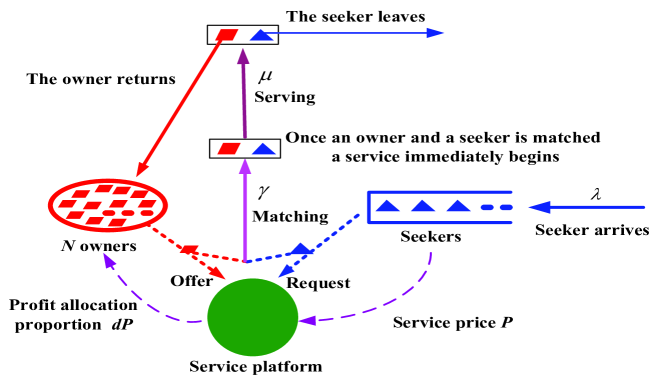
Figure 1: The queueing structure of service platforms

Remark 1.

Our queueing models have broad applications in the sharing economy (or the service platform). In a bike-sharing system, the owners are bikes, and the seekers are riders. In a car-sharing system, the owners are cars, and the seekers are drivers. In Didi Taxi or Uber, the owners are taxis, and the seekers are passengers. In a house-sharing system, the owners are houses or rooms, and the seekers are tenants. In an equipment-sharing system, the owners are equipments, and the seekers are customers.

3 A QBD Process and Stability

In this section, we express the first queueing model of service platforms as a level-independent QBD process, and obtain a necessary and sufficient condition under which this system is stable.

We denote by $N_{1}\left(t\right)$ and $N_{2}\left(t\right)$ the number of seekers waiting for their services, and the number of idle owners retained in the service platform at time $t\geq 0$, respectively. Note that the information completed in a service platform is observed at the matching completion time (it is also the service beginning time), the first queueing model of service platforms is modeled as a continuous-time Markov process $\left\{\left(N_{1}\left(t\right),N_{2}\left(t\right)\right),\text{ }t\geq 0\right\}$ whose state space is given by

$$\Omega=\bigcup\limits_{k=0}^{\infty}S_{k},$$

where the $0$th level is

$$S_{0}=\bigcup\limits_{i=0}^{N-1}\left\{\left(i,0\right),\left(i,1\right),\left(i,2\right),...,\left(i,N\right)\right\},$$

and for $k\geq 1$, the $k$th level is

$$S_{k}=\left\{\left(N+k-1,0\right),\left(N+k-1,1\right),...,\left(N+k-1,N\right)\right\}.$$

Since the information completed in a service platform is observed at the matching completion time (it is also the service beginning time), we can understand such special state transitions:

$$\left(k,k\right)\text{ }\underrightarrow{k\gamma}\text{ }\left(k-1,k-1\right),\text{ \ }k\geq 1,$$

$$\left(k,k+j\right)\text{ }\underrightarrow{k\gamma}\text{ }\left(k-1,k+j-1\right),\text{ \ }k\geq 1,j\geq 1,$$

$$\left(k+j,k\right)\text{ }\underrightarrow{k\gamma}\text{ }\left(k+j-1,k-1\right),\text{ \ }k\geq 1,j\geq 1.$$

Based on this finding, the state transition relations of the Markov process $\left\{\left(N_{1}\left(t\right),N_{2}\left(t\right)\right),\text{ }t\geq 0\right\}$ are depicted in Figure 2.

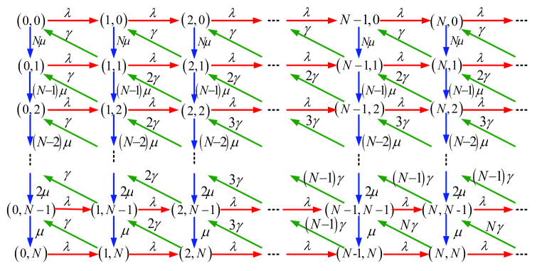
Figure 2: The state transition relations of the Markov process in Model one

It can be seen from Figure 2 that the infinitesimal generator of the Markov process $\{(N_{1}\left(t\right),N_{2}\left(t\right)),$ $t\geq 0\}$ is given by

$$Q=\left(\begin{array}[c]{cccccc}B_{0}&C_{0}&&&&\\ A_{0}&B&C&&&\\ &A&B&C&&\\ &&A&B&C&\\ &&&\ddots&\ddots&\ddots\end{array}\right),$$ (1)

where the repeated blocks are given by

$$A=\left(\begin{array}[c]{cccccc}0&&&&&\\ \gamma&0&&&&\\ &2\gamma&0&&&\\ &&\ddots&\ddots&&\\ &&&\left(N-1\right)\gamma&0&\\ &&&&N\gamma&0\end{array}\right),\text{ }C=\left(\begin{array}[c]{cccccc}\lambda&&&&&\\ &\lambda&&&&\\ &&\lambda&&&\\ &&&\ddots&&\\ &&&&\lambda&\\ &&&&&\lambda\end{array}\right),$$

$$B=\left(\begin{array}[c]{cccccc}b^{\left(0\right)}&N\mu&&&&\\ &b^{\left(1\right)}&\left(N-1\right)\mu&&&\\ &&b^{\left(2\right)}&\left(N-2\right)\mu&&\\ &&&\ddots&\ddots&\\ &&&&b^{\left(N-1\right)}&\mu\\ &&&&&b^{\left(N\right)}\end{array}\right);$$

$$b^{\left(i\right)}=-\left[\lambda+\left(N-i\right)\mu+i\gamma\right],\text{ \ \ }0\leq i\leq N;$$

and the boundary blocks are given by

$$A_{0}=\left(\begin{array}[c]{cccc}0&\cdots&0&B_{2}^{\left(N\right)}\end{array}\right),\text{ \ }C_{0}=\left(\begin{array}[c]{c}0\\ \vdots\\ 0\\ B_{0}^{\left(N-1\right)}\end{array}\right),$$

$$B_{0}=\left(\begin{array}[c]{cccccc}B_{1}^{\left(0\right)}&B_{0}^{\left(0\right)}&&&&\\ B_{2}^{\left(1\right)}&B_{1}^{\left(1\right)}&B_{0}^{\left(1\right)}&&&\\ &B_{2}^{\left(2\right)}&B_{1}^{\left(2\right)}&B_{0}^{\left(2\right)}&&\\ &&\ddots&\ddots&\ddots&\\ &&&B_{2}^{\left(N-2\right)}&B_{1}^{\left(N-2\right)}&B_{0}^{\left(N-2\right)}\\ &&&&B_{2}^{\left(N-1\right)}&B_{1}^{\left(N-1\right)}\end{array}\right),$$

$$B_{0}^{\left(k\right)}=\left(\begin{array}[c]{ccc}\lambda&&\\ &\ddots&\\ &&\lambda\end{array}\right),\text{ \ }0\leq k\leq N-1,\text{\ }$$

$$B_{2}^{\left(k\right)}=\left(\begin{array}[c]{cccccccc}0&&&&&&&\\ \gamma&0&&&&&&\\ &2\gamma&0&&&&&\\ &&\ddots&\ddots&&&&\\ &&&\left(k-1\right)\gamma&0&&&\\ &&&&k\gamma&0&&\\ &&&&&\ddots&0&\\ &&&&&&k\gamma&0\end{array}\right),\text{ \ }1\leq k\leq N,$$

and for $0\leq k\leq N-1$

$$B_{1}^{\left(k\right)}=\left(\begin{array}[c]{cccccccc}c^{\left(0\right)}&N\mu&&&&&&\\ &c^{\left(1\right)}&\left(N-1\right)\mu&&&&&\\ &&\ddots&\ddots&&&&\\ &&&c^{\left(k-1\right)}&\left(N-k+1\right)\mu&&&\\ &&&&c^{\left(k\right)}&\left(N-k\right)\mu&&\\ &&&&&\ddots&\ddots&\\ &&&&&&c^{\left(N-1\right)}&\mu\\ &&&&&&&c^{\left(N\right)}\end{array}\right),$$

$$c^{\left(i\right)}=\left\{\begin{array}[c]{ll}-\left[\lambda+i\gamma+\left(N-i\right)\mu)\right],&0\leq i\leq k-1,\\ -\left[\lambda+k\gamma+\left(N-i\right)\mu)\right],&k\leq i\leq N.\end{array}\right.$$

It is easy to see from the infinitesimal generator $Q$ that the Markov process $\{(N_{1}\left(t\right),N_{2}\left(t\right)),$ $t\geq 0\}$ is an irreducible QBD process.

To find the stable condition of the QBD process $Q$, the following lemma is useful in our later computation. The first equation in Lemma 1 is straightforward by means of the Newton binomial theorem, and the second equation can be obtained by taking the derivatives in both sides of the first equation.

Lemma 1.

For $x>0$, we have

$$\sum\limits_{i=0}^{N}C_{N}^{i}x^{i}=\left(1+x\right)^{N}$$

and

$$\sum\limits_{i=1}^{N}iC_{N}^{i}x^{i}=Nx\left(1+x\right)^{N-1}.$$

The following theorem provides a necessary and sufficient condition under which the QBD process $Q$ is stable.

Theorem 1.

The QBD process $Q$ is positive recurrent if and only if $\rho=\lambda\left(1+\mu/\gamma\right)/N\mu<1$. Also, the first queueing model of the service platforms is stable.

Proof. It is easy to identify the irreducibility of the QBD process $Q$ from Figure 2.

To prove that the QBD process $Q$ is positive recurrent, it is the key to find a necessary and sufficient condition by using the mean drift technique by Neuts [41].

Let $D=A+B+C$. Then

$$D=\left(\begin{array}[c]{cccccc}d^{\left(0\right)}&N\mu&&&&\\ \gamma&d^{\left(1\right)}&\left(N-1\right)\mu&&&\\ &2\gamma&d^{\left(2\right)}&\left(N-2\right)\mu&&\\ &&\ddots&\ddots&\ddots&\\ &&&\left(N-1\right)\gamma&d^{\left(N-1\right)}&\mu\\ &&&&N\gamma&d^{\left(N\right)}\end{array}\right),$$

where

$$d^{\left(i\right)}=-\left[\left(N-i\right)\mu+i\gamma\right],\text{ \ }0\leq i\leq N.$$

Note that the Markov process $D$ is irreducible and has finite states. Thus, it is positive recurrent. Let $\alpha=\left(\alpha_{1},\alpha_{2},\alpha_{3},\ldots,\alpha_{N+1}\right)$ be the stationary probability vector of the Markov process $D$. Then

$$\alpha D=\mathbf{0},\text{ \ }\alpha\mathbf{e}=1,$$

where $\mathbf{0}$ is a zero row vector with a suitable sizes (here, size $N+1)$, and $\mathbf{e}$ is a column vector of ones with a suitable sizes (here, size $N+1)$. Note that $\alpha>0$ is due to the fact that the Markov process $D$ is irreducible.

Once the stationary probability vector $\alpha$ is obtained, we can compute the (upward and downward) mean drift rates of the QBD process $Q$. From level $i$ to level $i+1$, the upward mean drift rate is given by

$$\alpha C\mathbf{e=}\lambda\alpha\mathbf{e}=\lambda,$$

since $C=\lambda I$ and $\alpha\mathbf{e}=1$, where $I$ is an identity matrix.

Similarly, from level $i$ to level $i-1$, the downward mean drift rate is $\alpha A\mathbf{e}$. To compute the drift rate $\alpha A\mathbf{e}$, we need to solve the system of linear equations: $\alpha D=\mathbf{0}$ and $\alpha\mathbf{e}=1$ as follows:

$$\alpha_{1}=\frac{1}{\sum\limits_{i=0}^{N}C_{N}^{i}\left(\frac{\mu}{\gamma}\right)^{i}},$$

and for $2\leq k\leq N+1$,

$$\alpha_{k}=C_{N}^{k-1}\left(\frac{\mu}{\gamma}\right)^{k-1}\alpha_{1}=\frac{C_{N}^{k-1}\left(\frac{\mu}{\gamma}\right)^{k-1}}{\sum\limits_{i=0}^{N}C_{N}^{i}\left(\frac{\mu}{\gamma}\right)^{i}}.$$

Now, we compute

$$\alpha A\mathbf{e} =1\gamma\alpha_{2}+2\gamma\alpha_{3}+\cdots+N\gamma\alpha_{N+1}$$

$$=\frac{\gamma\sum\limits_{i=1}^{N}iC_{N}^{i}\left(\frac{\mu}{\gamma}\right)^{i}}{\sum\limits_{i=0}^{N}C_{N}^{i}\left(\frac{\mu}{\gamma}\right)^{i}}=\frac{N\mu\gamma}{\mu+\gamma}.$$

Let $\rho=\left(\alpha C\mathbf{e}\right)/\left(\alpha A\mathbf{e}\right)$. Then

$$\rho=\frac{\lambda\left(\mu+\gamma\right)}{N\mu\gamma}.$$

It is clear that $\alpha C\mathbf{e<}$ $\alpha A\mathbf{e}$ if and only if $\rho<1$. Therefore, the QBD process $Q$ is positive recurrent if and only if $\rho<1$ or $\alpha C\mathbf{e<}$ $\alpha A\mathbf{e}$. This completes the proof. $\blacksquare$

The following corollary provides a novel stable condition under which the QBD process $Q$ is positive recurrent. We show that the first queueing model of service platforms is always stable as long as the number $N$ of independent owners is large enough. Such a result is not intuitive but it is very useful in the design of a service platform whose normal operation needs to have enough independent owners.

Corollary 2.

If $N>1+\left\lfloor\frac{\lambda}{\mu}\left(1+\frac{\mu}{\gamma}\right)\right\rfloor$, where $\left\lfloor x\right\rfloor$ is the maximum integer lower than or equal to $x$, then the QBD process $Q$ (or the first queueing model of service platforms) must be positive recurrent.

Proof. We only need to observe that if $N>1+\left\lfloor\frac{\lambda}{\mu}\left(1+\frac{\mu}{\gamma}\right)\right\rfloor$, then $\rho<1$. This completes the proof. $\blacksquare$

4 Performance Measures

In this section, we apply the matrix-geometric solution to give the stationary probability vector of the QBD process, and provide some useful performance measures of the service platform.

We write

$$p_{i,j}\left(t\right)=P\left\{N_{1}\left(t\right)=i,N_{2}\left(t\right)=j\right\}.$$

Since the QBD process is stable, we have

$$\pi_{i,j}=\lim_{t\rightarrow+\infty}p_{i,j}\left(t\right).$$

For $k=0$, we write

$$\pi_{0}=\left(\pi_{0}^{\left(0\right)},\pi_{0}^{\left(1\right)},\pi_{0}^{\left(2\right)},\ldots,\pi_{0}^{\left(N-1\right)}\right)$$

,

$$\pi_{0}^{\left(i\right)}=\left(\pi_{i,0},\pi_{i,1},\ldots,\pi_{i,N}\right),\text{ \ }0\leq i\leq N-1;$$

for $k\geq 1$, we write

$$\pi_{k}=\left(\pi_{N+k-1,0},\pi_{N+k-1,1},\pi_{N+k-1,2},\ldots,\pi_{N+k-1,N}\right),$$

and

$$\pi=\left(\pi_{0},\pi_{1},\pi_{2},\ldots\right).$$

If $\pi=\left(\pi_{0},\pi_{1},\pi_{2},\ldots\right)$ is the stationary probability vector of the QBD process $Q$, then $\pi$ satisfies the system of linear equations:

$$\pi Q=\mathbf{0,}\text{ \ }\pi\mathbf{e}=1,$$ (2)

which leads to

$$\pi_{0}B_{0}+\pi_{1}A_{0}=0,$$ (3)

$$\pi_{0}C_{0}+\pi_{1}B+\pi_{2}A=0,$$ (4)

$$\pi_{k-1}C+\pi_{k}B+\pi_{k+1}A=0,\text{ \ }k\geq 2,$$ (5)

$$\sum\limits_{k=0}^{\infty}\pi_{k}\mathbf{e}=1.$$ (6)

Let the matrix rate $R$ be the minimal non-negative solution to the matrix quadratic equation

$$R^{2}A+RB+C=0.$$ (7)

The following theorem can directly be obtained by using Chapter 3 of Neuts [41].

Theorem 3.

The stationary probability vector of the QBD process $Q$ is a matrix-geometric solution

$$\pi_{i}=\pi_{1}R^{i-1},\text{ }i\geq 1,$$ (8)

where $\left(\pi_{0},\pi_{1}\right)$ is the unique solution to the following system of linear equations

$$\pi_{0}B_{0}+\pi_{1}A_{0}=0,$$

$$\pi_{0}C_{0}+\pi_{1}\left(B+RA\right)=0$$

and

$$\pi_{0}e+\pi_{1}\left(I-R\right)^{-1}\mathbf{e}=1.$$

4.1 The stationary performance measures

In this subsection, by using the stationary probability vector of the QBD process $Q$, we provide some useful performance measures of the first queueing model of service platforms, e.g., the stationary average numbers, and the expected profits of the platform and each owner.

(a) The stationary average numbers

Let $\mathcal{Q}^{\left(1\right)}$ and $\mathcal{Q}^{\left(2\right)}$ denote the stationary numbers of the idle owners retained in the service platform, and of the seekers waiting for their services, respectively. Then

$$E\left[\mathcal{Q}^{\left(1\right)}\right] =\sum\limits_{i=0}^{\infty}\sum\limits_{j=1}^{N}j\pi_{i,j}$$

$$=\sum_{l=0}^{N-1}\pi_{0}^{\left(l\right)}f+\pi_{1}\left(I-R\right)^{-1}f,$$ (9)

where $f=\left(0,1,2,\ldots,N\right)^{T}$, and

$$E\left[\mathcal{Q}^{\left(2\right)}\right] =\sum\limits_{i=1}^{\infty}\sum\limits_{j=0}^{N}i\pi_{i,j}$$

$$=\pi_{1}\left(I-R\right)^{-1}\mathbf{e}.$$ (10)

(b) The expected profits of the service platform and each owner

Let $f_{1}$ and $f_{2}$ denote the expected profits per unit time of the service platform and each owner, respectively. Then by using the service price $P$ and the profit allocation proportion $d$, we have

$$f_{1}=\left(1-d\right)\cdot P\left(N-E\left[\mathcal{Q}^{\left(1\right)}\right]\right)\mu,$$

and

$$f_{2} =\frac{1}{N}d\cdot P\left(N-E\left[\mathcal{Q}^{\left(1\right)}\right]\right)\mu$$

$$=d\cdot P\left(1-\frac{1}{N}E\left[\mathcal{Q}^{\left(1\right)}\right]\right)\mu,$$

where $E\left[\mathcal{Q}^{\left(1\right)}\right]$ is given in (9). Note that $N-E\left[\mathcal{Q}^{\left(1\right)}\right]$ is the average number of the busy owners, and $P\left(N-E\left[\mathcal{Q}^{\left(1\right)}\right]\right)\mu$ is the total expected profits per unit time of the service platform, which is paid by all the seekers served per unit time.

4.2 The sojourn time of an arriving seeker

In this subsection, we compute the expected sojourn time of each arriving seeker at the service platform. That is, the sojourn time begins from the moment of the seeker entering the service platform to the epoch that the seeker leaves the system after receiving his/her service from the owner.

We denote by $W$ the sojourn time of an arriving seeker at the service platform. To compute the expected sojourn time $E\left[W\right]$, we need to apply the first passage time of the QBD process with an absorbing state. To this end, we revise the QBD process $\left\{\left(N_{1}\left(t\right),N_{2}\left(t\right)\right),\text{ }t\geq 0\right\}$ as a QBD process with an absorbing state

$$\Delta=\left\{\left(0,0\right),\left(0,1\right),\left(0,2\right),...,\left(0,N-1\right)\right\},$$

while state $\left(0,N\right)$ is a sliding state and is mitted here. Thus, the QBD process with the absorption state $\Delta$ is depicted in Figure 3. Based on this, the state space of the QBD process with the absorbing state is given by

$$\widetilde{\Omega}=\left\{\Delta\right\}\cup\widetilde{S}_{0}\cup\left\{\bigcup\limits_{i=1}^{\infty}S_{i}\right\},$$

where

$$\widetilde{S}_{0}=\bigcup\limits_{i=1}^{N-1}\left\{\left(i,0\right),\left(i,1\right),\left(i,2\right),...,\left(i,N\right)\right\},$$

and for $k\geq 1$,

$$S_{k}=\left\{\left(N+k-1,0\right),\left(N+k-1,1\right),...,\left(N+k-1,N\right)\right\}.$$

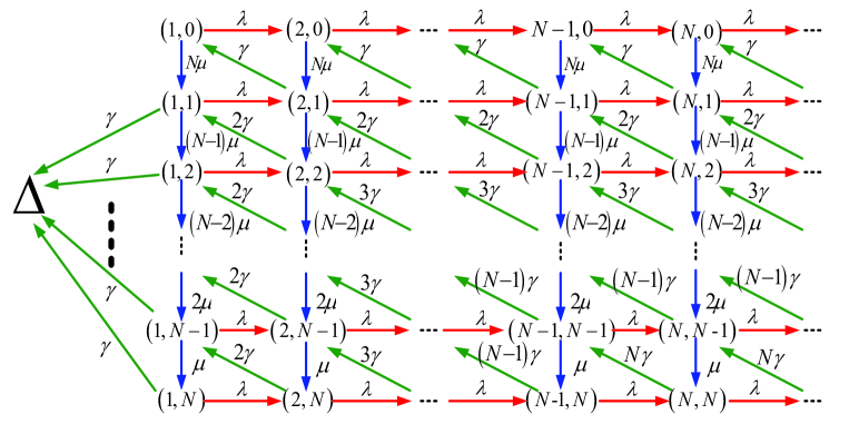
Figure 3: The state transition relations of the QBD process with an absorbing state

From Figure 3, it is seen that the infinitesimal generator of the QBD process with the absorption state $\Delta$ is given by

$$\mathbf{Q}=\left(\begin{array}[c]{cccccc}0&\mathbf{0}&\mathbf{0}&\mathbf{0}&\mathbf{0}&\cdots\\ \widetilde{\varphi}&\widetilde{B}_{0}&\widetilde{C}_{0}&&&\\ &\widetilde{A}_{0}&B&C&&\\ &&A&B&C&\\ &&&\ddots&\ddots&\ddots\end{array}\right)$$ (11)

where the blocks $A$, $B$ and $C$ are the same as those given in matrix $Q$, and

$$\widetilde{B}_{0}=\left(\begin{array}[c]{cccccc}B_{1}^{\left(1\right)}&B_{0}^{\left(1\right)}&&&&\\ B_{2}^{\left(2\right)}&B_{1}^{\left(2\right)}&B_{0}^{\left(2\right)}&&&\\ &\ddots&\ddots&\ddots&&\\ &&&B_{2}^{\left(N-2\right)}&B_{1}^{\left(N-2\right)}&B_{0}^{\left(N-2\right)}\\ &&&&B_{2}^{\left(N-1\right)}&B_{1}^{\left(N-1\right)}\end{array}\right),$$

$$\widetilde{A}_{0}=\left(\begin{array}[c]{cccc}0&\cdots&0&B_{2}^{\left(N\right)}\end{array}\right),\text{ \ }\widetilde{C}_{0}=\left(\begin{array}[c]{c}0\\ \vdots\\ 0\\ B_{0}^{\left(N-1\right)}\end{array}\right),$$

$$\widetilde{\varphi}=\left(\begin{array}[c]{c}\varphi\\ 0\\ \vdots\\ 0\end{array}\right),\text{ \ }\varphi=\left(\begin{array}[c]{c}0\\ \gamma\\ \vdots\\ \gamma\end{array}\right).$$

Let

$$T=\left(\begin{array}[c]{ccccc}\widetilde{B}_{0}&\widetilde{C}_{0}&&&\\ \widetilde{A}_{0}&B&C&&\\ &A&B&C&\\ &&\ddots&\ddots&\ddots\end{array}\right),\text{ \ }T^{0}=\left(\begin{array}[c]{c}\widetilde{\varphi}\\ 0\\ 0\\ \vdots\end{array}\right).$$

Then the infinitesimal generator $\mathbf{Q}$ can be abbreviated as

$$\mathbf{Q}=\left(\begin{array}[c]{cc}0&\mathbf{0}\\ T^{0}&T\end{array}\right).$$ (12)

It is easy to see that $T\mathbf{e}+T^{0}=0$.

Now, the initial probability vector of the QBD process $\mathbf{Q}$ with the absorption state $\Delta$ is written as

$$\omega=\left(\omega_{\triangle},\widetilde{\omega}\right),$$

where $\omega_{\triangle}$ is a scalar, and $\omega_{0}^{\left(i\right)}$ for $1\leq i\leq N-1$ and $\omega_{k}$ for $k\geq 1$ are row vectors of size $N+1$,

$$\widetilde{\omega}=\left(\omega_{0},\omega_{1},\omega_{2},\ldots\right),$$

$$\omega_{0}=\left(\omega_{0}^{\left(1\right)},\omega_{0}^{\left(2\right)},\omega_{0}^{\left(3\right)},\ldots,\omega_{0}^{\left(N-1\right)}\right),$$

with

$$\omega_{\triangle}+\sum_{i=1}^{N-1}\omega_{0}^{\left(i\right)}\mathbf{e}+\sum_{k=1}^{\infty}\omega_{k}\mathbf{e}=1,$$

By using the stationary probability vector $\pi=\left(\pi_{0},\pi_{1},\pi_{2},\ldots\right)$, we can set up a key initial probability vector

$$\omega=\left(\omega_{\triangle};\omega_{0}^{\left(1\right)},\omega_{0}^{\left(2\right)},\omega_{0}^{\left(3\right)},\ldots,\omega_{0}^{\left(N-1\right)};\omega_{1},\omega_{2},\ldots\right),$$

where

$$\omega_{\triangle} =\pi_{0}^{\left(0\right)}\mathbf{e,}$$

$$\omega_{0}^{\left(i\right)} =\pi_{0}^{\left(i\right)},\text{ }1\leq i\leq N-1,$$

$$\omega_{k} =\pi_{k},\text{ \ }k\geq 1.$$

The following theorem uses the phase-type distribution of infinite size to provide expression for the probability distribution of the sojourn time $W$.

Theorem 4.

If the initial probability vector of the QBD process $\mathbf{Q}$ with the absorption state $\Delta$ is $\omega=\left(\omega_{\triangle},\widetilde{\omega}\right)$, then

(1) the probability distribution of the sojourn time $W$ is of phase type with an irreducible representation $\left(\widetilde{\omega},T\right)$, i.e.,

$$F_{W}\left(t\right)=P\left\{W\leq t\right\}=1-\omega_{\triangle}-\widetilde{\omega}\exp\left\{Tt\right\}\mathbf{e,}\text{ \ }t\geq 0;$$

(2) the expected sojourn time

$$E\left[W\right]=\widetilde{\omega}\left(-T\right)_{\min}^{-1}\mathbf{e,}$$

where $\left(-T\right)_{\min}^{-1}$ is the minimal nonnegative inverse matrix of the matrix $-T$.

Proof. (1) For $i=1,2,3,...$, and $j=1,2,3,...,N$, we write

$$q_{i,j}\left(t\right)=P\left\{N_{1}\left(t\right)=i,N_{2}\left(t\right)=j\right\},$$

For $k=0$, we write

$$q_{0}\left(t\right)=\left(q_{0}^{\left(1\right)}\left(t\right),q_{0}^{\left(2\right)}\left(t\right),q_{0}^{\left(3\right)}\left(t\right),\ldots,q_{0}^{\left(N-1\right)}\left(t\right)\right)$$

,

$$q_{0}^{\left(i\right)}\left(t\right)=\left(q_{i,1}\left(t\right),q_{i,2}\left(t\right),q_{i,3}\left(t\right),\ldots,q_{i,N}\left(t\right)\right),\text{ \ }1\leq i\leq N-1;$$

for $k\geq 1$, we write

$$q_{k}\left(t\right)=\left(q_{N+k-1,0}\left(t\right),q_{N+k-1,1}\left(t\right),q_{N+k-1,2}\left(t\right),\ldots,q_{N+k-1,N}\left(t\right)\right),$$

and

$$q\left(t\right)=\left(q_{0}\left(t\right),q_{1}\left(t\right),q_{2}\left(t\right),\ldots\right).$$

It follows from the Chapman-Kolmogorov forward equation that

$$\frac{d}{dt}q\left(t\right)=q\left(t\right)T,$$ (13)

with the initial condition

$$q\left(0\right)=\widetilde{\omega}.$$ (14)

It follows from (13) and (14) that

$$q\left(t\right)=\widetilde{\omega}e^{Tt}.$$ (15)

Note that $q\left(0\right)\mathbf{e}=1-\omega_{\triangle}$. We then obtain

$$F_{W}\left(t\right) =P\left\{W\leq t\right\}=1-\omega_{\triangle}-q\left(t\right)\mathbf{e}$$

$$=1-\omega_{\triangle}-\widetilde{\omega}\exp\left(Tt\right)\mathbf{e,}\text{ }t\geq 0.$$

(2) Now, we compute the expected sojourn time $E\left[W\right]$ by the Laplace-Stieltjes transform. Let $f\left(s\right)$ be the Laplace-Stieltjes transform of the distribution function $F_{W}\left(t\right)$ or the random variable $W$. Then

$$f\left(s\right) =\int\nolimits_{0}^{\infty}e^{-st}dF_{W}(t)$$

$$=1-\omega_{\triangle}+\widetilde{\omega}\left(sI-T\right)_{\min}^{-1}T^{0},$$ (16)

where $\left(sI-T\right)_{\min}^{-1}$ is the minimal nonnegative inverse of the matrix $sI-T$ of infinite size. It is easy to see that

$$E\left[W\right]=-\frac{d}{ds}f\left(s\right)_{\mid s=0}=\widetilde{\omega}\left[\left(sI-T\right)_{\min}^{-2}\right]_{\mid s=0}T^{0}=\widetilde{\omega}\left(-T\right)_{\min}^{-1}\mathbf{e,}$$ (17)

by using $T\mathbf{e}+T^{0}=0$ and $\left(-T\right)_{\min}^{-1}\left(-T\right)\mathbf{e=e}$. This completes the proof. $\blacksquare$

In the remainder of this section, we use the RG-factorizations by Li [36] to compute the expected sojourn time $E\left[W\right]$. It is easy to see that the key is how to deal with the minimal nonnegative inverse matrix $\left(-T\right)_{\min}^{-1}$ of the matrix $-T$ of infinite size. To this end, we write

$$T=\left(\begin{array}[c]{c}T_{1,1}\text{ }T_{1,2}\\ T_{2,1}\text{ }T_{2,2}\end{array}\right),$$

where

$$T_{1,1}=\widetilde{B}_{0},\text{ \ }T_{1,2}=\left(\begin{array}[c]{ccccc}\widetilde{C}_{0}\text{ }&&&&\end{array}\text{\ }\right),\text{ \ }T_{2,1}=\widetilde{A}_{0},$$

$$T_{2,2}=\left(\begin{array}[c]{ccccc}B&C&&&\\ A&B&C&&\\ &A&B&C&\\ &&\ddots&\ddots&\ddots\end{array}\right).$$

Note that the QBD process $Q$ is irreducible, and thus matrix $T$ and $T_{2,2}$ must be invertible. Here, we take that $T^{-1}=T_{\max}^{-1}$ and $T_{2,2}^{-1}=\left(T_{2,2}^{-1}\right)_{\max}$, i.e., their inverse matrices are maximal non-positive. Based on this, it is easy to check that

$$T^{-1}=\left[\begin{array}[c]{cc}T_{1,1;2}^{-1}&-T_{1,1;2}^{-1}T_{1,2}T_{2,2}^{-1}\\ -T_{2,2}^{-1}T_{2,1}T_{1,1;2}^{-1}&T_{2,2}^{-1}+T_{2,2}^{-1}T_{2,1}T_{1,1;2}^{-1}T_{1,2}T_{2,2}^{-1}\end{array}\right],$$ (18)

where

$$T_{1,1;2}=T_{1,1}-T_{1,2}T_{2,2}^{-1}T_{2,1}.$$ (19)

It is clear that the inverse matrix $T^{-1}$ can be expressed by means of the inverse matrix $T_{2,2}^{-1}$ of matrix $T_{2,2}$. This relation plays a key role in setting up the PH distribution of infinite sizes with an irreducible representation $\left(\widetilde{\omega},T\right)$.

To compute the inverse matrix $T_{2,2}^{-1}$ of infinite sizes, we define the UL-type $U$-, $R$- and $G$-measures as follows. Let $R$ and $G$ be the minimal non-negative solutions to the matrix quadratic equations

$$R^{2}A+RB+C=0$$ (20)

and

$$A+BG+CG^{2}=0,$$ (21)

respectively. The $U$-measure is given by

$$U=B+RA=B+CG\text{.}$$ (22)

Now, we can provide the UL-type RG-factorization of the Markov process $T_{2,2}$ of infinite size as follows:

$$T_{2,2}=\left(I-R_{U}\right)U_{D}\left(I-G_{L}\right),$$ (23)

where

$$I-R_{U}=\left(\begin{array}[c]{ccccc}I&-R&&&\\ &I&-R&&\\ &&I&-R&\\ &&&I&\ddots\\ &&&&\ddots\end{array}\right),$$ (24)

$$U_{D}=\text{diag}\left(U,U,U,U,\ldots\right),$$ (25)

$$I-G_{L}=\left(\begin{array}[c]{ccccc}I&&&&\\ -G&I&&&\\ &-G&I&&\\ &&-G&I&\\ &&&\ddots&\ddots\end{array}\right).$$ (26)

It is easy to check that the matrices $I-R_{U}$, $U_{D}$, and $I-G_{L}$ are invertible, and

$$\left(I-R_{U}\right)^{-1}=\left(\begin{array}[c]{ccccc}I&R&R^{2}&R^{3}&\ldots\\ &I&R&R^{2}&\ldots\\ &&I&R&\ldots\\ &&&I&\ldots\\ &&&&\ddots\end{array}\right),$$ (27)

$$U_{D}^{-1}=\text{diag}\left(U^{-1},U^{-1},U^{-1},U^{-1},\ldots\right),$$ (28)

$$\left(I-G_{L}\right)^{-1}=\left(\begin{array}[c]{ccccc}I&&&&\\ G&I&&&\\ G^{2}&G&I&&\\ G^{3}&G^{2}&G&I&\\ \vdots&\vdots&\vdots&\vdots&\ddots\end{array}\right).$$ (29)

By using the RG-factorization (23), we obtain

$$T_{2,2}^{-1}=\left(I-G_{L}\right)^{-1}U_{D}^{-1}\left(I-R_{U}\right)^{-1}.$$ (30)

By means of (18), (19), and (30), we can obtain the inverse matrix $T^{-1}$.

5 The Second Queueing Model

In this section, we provide a simple analysis for the second queueing model of service platforms by using the level-independent QBD process.

We first observe the matching and service processes. Let $X$ and $Y$ be two exponential random variables with the means $1/\gamma$ and $1/\mu$, respectively. Then the sum $X+Y$ follows a generalized Erlang distribution of order $2$, or $X+Y$ also follows a phase-type (PH) distribution of order $2$ under a more general setting. Here, $X$ and $Y$ are regarded as Phases $1$ and $2$ of the PH distribution, respectively. For the generalized Erlang distribution of order $2$, we write

$$\alpha=\left(1,0\right),\text{ }T=\left(\begin{array}[c]{cc}-\gamma&\gamma\\ 0&-\mu\end{array}\right),\text{ }T^{0}=\left(\begin{array}[c]{c}0\\ \mu\end{array}\right),\text{ }\mathbf{e}=\left(\begin{array}[c]{c}1\\ 1\end{array}\right).$$

For $2\leq n\leq N$

$$T\left(n\right)=\underset{\text{Keronecker sum of }n\text{ matrices }T}{\underbrace{T\oplus T\oplus\cdots\oplus T};}$$

for $2\leq k\leq N-1$

$$C\left(k+1\right)= T^{0}\otimes\underset{\text{Keronecker product of }k\text{ identity matrices}}{\underbrace{I\otimes I\otimes\cdots\otimes I}}+\mathbf{e}\otimes\left(T^{0}\alpha\right)\otimes I\otimes\cdots\otimes I+\cdots$$

$$+\mathbf{e}\otimes I\otimes\cdots\otimes\left(T^{0}\alpha\right)\otimes I+\mathbf{e}\otimes I\otimes I\otimes\cdots\otimes\left(T^{0}\alpha\right),$$

and for $1\leq l\leq N-1$

$$D\left(l\right)=\underset{\text{Keronecker product of }l\text{ identity matrix}}{\underbrace{I\otimes I\otimes\cdots\otimes I}}\otimes\alpha,$$

For the second queueing model of service platforms, the information completed in a service platform is observed at the matching beginning time. Thus, the sum $X+Y$ of the matching and service times is regarded as a generalized service time, which follows a generalized Erlang distribution of order $2$ (abbreviated as $\widetilde{\text{E}}_{2}$). In this case, the second queueing model of service platforms can be regarded as an M$/\widetilde{\text{E}}_{2}/N$ queue (or an M$/$PH$/N$ queue).

To study the M$/\widetilde{\text{E}}_{2}/N$ queue, we denote by $N\left(t\right)$ and $M\left(t\right)$ the number of seekers waiting for their services, and the number of working owners at time $t\geq 0$, respectively. If $N\left(t\right)=0$, then $0\leq M\left(t\right)\leq N$; and if $N\left(t\right)\geq 1$, then $M\left(t\right)=N$. Let $J\left(t\right)$ be the phase of the generalized Erlang service time $\widetilde{\text{E}}_{2}$ at time $t$. Then $J\left(t\right)\in\left\{1,2\right\}$. It is easy to see that $\left\{N\left(t\right),\underset{\text{the number of }J\left(t\right)\text{s is }M\left(t\right)}{M\left(t\right),\underbrace{J\left(t\right),J\left(t\right),\ldots,J\left(t\right)}}\right\}$ is a level-independent QBD process whose infinitesimal generator is given by

$$\mathbb{Q}=\left(\begin{array}[c]{ccccc}F_{1}&F_{0}&&&\\ F_{2}&A_{1}&A_{0}&&\\ &A_{2}&A_{1}&A_{0}&\\ &&\ddots&\ddots&\ddots\end{array}\right),$$

where

$$F_{1}=\left(\begin{array}[c]{ccccc}-\lambda&\lambda\alpha\left(1\right)&&&\\ T^{0}&T-\lambda I&\lambda D\left(1\right)&&\\ &C\left(2\right)&T\left(2\right)-\lambda I\left(2\right)&\lambda D\left(2\right)&\\ &&\ddots&\ddots&\ddots\\ &&&C\left(N-1\right)&T\left(N-1\right)-\lambda I\left(N-1\right)\end{array}\right)$$

$$F_{0}=\left(\begin{array}[c]{ccccc}&&&&\\ &&&&\\ &&&&\\ \lambda D\left(N-1\right)&&&&\end{array}\right),\text{ \ \ }F_{2}=\left(\begin{array}[c]{ccccc}&&&&C\left(N\right)\end{array}\right);$$

$$A_{0}=\underset{\text{Keronecker product of }N\text{ identity matrices}}{\lambda\underbrace{I\otimes I\otimes\cdots\otimes I}},\text{\ }$$

$$A_{1}=\underset{\text{Keronecker sum of }N\text{ matrices }T}{\underbrace{T\oplus T\oplus\cdots\oplus T}}-\text{ }\underset{\text{Keronecker product of }N\text{ identity matrices}}{\lambda\underbrace{I\otimes I\otimes\cdots\otimes I},}$$

$$A_{2}= \left(T^{0}\alpha\right)\otimes\underset{\text{Keronecker product of }N-1\text{ identity matrices}}{\underbrace{I\otimes I\otimes\cdots\otimes I}}+\text{ }I\otimes\left(T^{0}\alpha\right)\otimes I\otimes\cdots\otimes I+\cdots$$

$$+I\otimes I\otimes\cdots\otimes\left(T^{0}\alpha\right)\otimes I+I\otimes I\otimes I\otimes\cdots\otimes\left(T^{0}\alpha\right).$$

Now, we apply the mean drift technique to find a necessary and sufficient condition under which the QBD process $\mathbb{Q}$ is stable.

Theorem 5.

The QBD process $\mathbb{Q}$ is stable if and only if $\rho=\left[\lambda\left(\gamma+\mu\right)\right]/\left(N\mu\gamma\right)<1$.

Proof. We compute

$$\mathbf{A}= A_{0}+A_{1}+A_{2}$$

$$= \underset{\text{Keronecker sum of }n\text{ matrices }T}{\underbrace{T\oplus T\oplus\cdots\oplus T}}+\underset{\text{Keronecker product of }N-1\text{ identity matrices}}{\left(T^{0}\alpha\right)\otimes\underbrace{I\otimes I\otimes\cdots\otimes I}}$$

$$+\cdots+I\otimes I\otimes I\otimes\cdots\otimes\left(T^{0}\alpha\right)$$

$$= \left(T+T^{0}\alpha\right)\otimes I\otimes I\otimes\cdots\otimes I+\cdots$$

$$+I\otimes I\otimes I\otimes\cdots\otimes\left(T+T^{0}\alpha\right).$$

Since the Markov process $T+T^{0}\alpha$ is irreducible and positive recurrent, it has one unique stationary probability vector $\omega=\left(\omega_{1},\omega_{2}\right)$, where

$$\omega_{1}=\frac{\mu}{\gamma+\mu},\text{ \ }\omega_{2}=\frac{\gamma}{\gamma+\mu}.$$

It is easy to check that $\Theta=\underset{\text{Keronecker product of }N\text{ vectors }\omega}{\underbrace{\omega\otimes\omega\otimes\cdots\otimes\omega}}$ is the stationary probability vector of the the Markov process $\mathbf{A}$. Also, we get

$$\Theta A_{2}e=N\mu\frac{\gamma}{\gamma+\mu},\text{ \ }\Theta A_{0}e=\lambda.$$

By using the mean drift technique, the QBD process $\mathbb{Q}$ is stable if and only if $\Theta A_{2}e>\Theta A_{0}e$. Note that $\Theta A_{2}e>\Theta A_{0}e$ is equivalent to

$$\rho=\frac{\lambda}{N\mu\frac{\gamma}{\gamma+\mu}}=\frac{\lambda\left(\gamma+\mu\right)}{N\mu\gamma}<1.$$

Therefore, we find a necessary and sufficient condition under which the QBD process $\mathbb{Q}$ is stable. This completes the proof. $\blacksquare$

If the QBD process $\mathbb{Q}$ is stable, then it must has a stationary probabilty vector

$$\Psi=\left(\psi_{0},\psi_{1},\psi_{2},\ldots\right),$$

where $\psi_{0}$ is related to Level $0$ corresponding to the matrix $B_{1}$, and $\psi_{k}$ is related to Level $k$ corresponding to the matrix $A_{1}$. To provide performance evaluation of the second queueing model of service platforms, we need to express each element of the stationary probabilty vector $\Psi$ according to the Keronecker sum and the Keronecker product in matrix computation involved.

It is a little more complicated to express the elements of the vector $\psi_{0}$. Corresponding to the matrix $B_{1}$ with the Keronecker sums and the Keronecker products, we have

$$\psi_{0}=\left(\psi_{0,(0)}^{\left(0\right)};\psi_{1,(1)}^{\left(0\right)},\psi_{1,(2)}^{\left(0\right)};\psi_{2,(1,1)}^{\left(0\right)},\psi_{2,(1,2)}^{\left(0\right)},\psi_{2,(2,1)}^{\left(0\right)},\psi_{2,(2,2)}^{\left(0\right)};\ldots\right).$$

For $1\leq n\leq N-1$, these elements $\psi_{n,(i_{1},i_{2},i_{3},\ldots,i_{n})}$ with $i_{k}=1$ or $2$ and for $1\leq k\leq n$ are arranged in a multi-dimensional lexicographic order. For the multi-dimensional lexicographic order, we provide two simple examples for $n=2,3$, while for the general case with $4\leq n\leq N-1$, we can similarly write such a lexicographic order.

Example one: $n=2$. In this case, $\psi_{2,(1,1)}^{\left(0\right)},\psi_{2,(1,2)}^{\left(0\right)},\psi_{2,(2,1)}^{\left(0\right)},\psi_{2,(2,2)}^{\left(0\right)}$.

Example two: $n=3$. In this case, $\psi_{3,(1,1,1)}^{\left(0\right)},\psi_{3,(1,1,2)}^{\left(0\right)},\psi_{3,(1,2,1)}^{\left(0\right)},\psi_{3,(1,2,2)}^{\left(0\right)},\psi_{3,(2,1,1)}^{\left(0\right)},\psi_{3,(2,1,2)}^{\left(0\right)}$, $\psi_{3,(2,2,1)}^{\left(0\right)},\psi_{3,(2,2,2)}^{\left(0\right)}$.

Now, we arrange the elements of the vector $\psi_{l}$ for $l\geq 1$. These elements $\psi_{N,(i_{1},i_{2},i_{3},\ldots,i_{N})}^{\left(l\right)}$ with $i_{k}=1$ or $2$ and for $1\leq k\leq N$ are arranged in the $N$-dimensional lexicographic order.

Note that $\Psi=\left(\psi_{0},\psi_{1},\psi_{2},\ldots\right)$ is the stationary probability vector of the QBD process $\mathbb{Q}$, then $\Psi$ satisfies the system of linear equations: $\Psi\mathbb{Q}=\mathbf{0\ }$and $\Psi e=1$.

Let the rate matrix $\mathbf{R}$ be the minimal non-negative solution to the matrix quadratic equation

$$\mathbf{R}^{2}A_{2}+\mathbf{R}A_{1}+A_{0}=0.$$

By using Chapter 3 of Neuts [41], the stationary probability of the QBD process $\mathbb{Q}$ is a matrix-geometric solution

$$\psi_{i}=\psi_{1}\mathbf{R}^{i-1},\text{ }i\geq 1,$$

where $\left(\psi_{0},\psi_{1}\right)$ is the unique solution to the following system of linear equations

$$\psi_{0}F_{1}+\psi_{1}F_{2}=0,$$

$$\psi_{0}F_{0}+\psi_{1}\left(A_{1}+\mathbf{R}A_{2}\right)=0$$

and

$$\psi_{0}e+\psi_{1}\left(I-\mathbf{R}\right)^{-1}e=1.$$

In the remainder of this section, by using the stationary probability vector of the QBD process $\mathbb{Q}$, we provide the performance measures of the second queueing model of service platforms as follows:

(a) The stationary average queue lengths

Let $\mathcal{Q}^{\left(1\right)}$ and $\mathcal{Q}^{\left(2\right)}$ denote the stationary queue lengths for the idle owners retained in the service platform, and for the seekers waiting for their services, respectively. Then

$$E\left[\mathcal{Q}^{\left(1\right)}\right]=\sum\limits_{n=0}^{N-1}\left(N-n\right)\sum\limits_{k=1}^{n}\sum_{i_{k}=1,2}\psi_{n,(i_{1},i_{2},i_{3},\ldots,i_{n})}$$

and

$$E\left[\mathcal{Q}^{\left(2\right)}\right]=\sum\limits_{k=1}^{\infty}k\Psi_{k}e=\Psi_{1}\left(I-R\right)^{-2}\mathbf{e}.$$

(b) The expected profits of the service platform and each owner

Let $f_{1}$ and $f_{2}$ denote the expected profits per unit time of a service platform and each owner, respectively. Then

$$f_{1}=\left(1-d\right)\cdot P\left(N-E\left[\mathcal{Q}^{\left(1\right)}\right]\right)\mu,$$

and

$$f_{2}=d\cdot P\left(1-\frac{1}{N}E\left[\mathcal{Q}^{\left(1\right)}\right]\right)\mu.$$

6 Numerical Examples

In this section, we uses numerical examples to discuss how the performance measures depend on some key system parameters. Note that the numerical analysis is useful and necessary in the design and operations management of the service platforms.

Note that the number of owners $N$ is a key factor that determines the sizes of blocks (for example, the matrices $A$, $B$ and $C$) in the infinitesimal generator $Q$. Also, the sizes of blocks directly affect algorithm design and computational complexity of the level-independent QBD process $Q$. Obviously, the larger the number $N$, the more difficult the numerical computation is.

In the first two parts (a) and (b), the selected parameters $\lambda$, $\mu$, $\gamma$ and $N$ must satisfy the system stable condition: $\rho=\lambda\left(1+\mu/\gamma\right)/N\mu<1$.

(a) The stationary average queue lengths

To obtain the stationary probability vector, we first need to compute the rate matrix $R$, which is the minimal nonnegative solution to the quadratic nonlinear matrix equation: $R^{2}A+RB+C=0$. A modified successive iteration method is found in, e.g., see Neuts [41] and Latouche and Ramaswami [34]. Now, we describe the modified successive iteration method as follows. The sequence $\left\{R\left(n\right);n\geq 0\right\}$ is designed as

$$R\left(0\right)=\mathbf{0,}$$

$$R\left(n+1\right)=-\left[R\left(n\right)^{2}A+C\right]B^{-1},\text{ \ \ }n=0,1,2,\ldots.$$

Neuts [41] indicated that $R\left(n\right)\uparrow R$ as $n\rightarrow\infty$. For any sufficiently small positive number $\varepsilon$ within the desired degree of accuracy, set at $10^{-12}$, if there exists a positive integer $n$ such that

$$\left\|R\left(n+1\right)-R\left(n\right)\right\|=\max\left|R\left(n+1\right)_{i,j}-R\left(n\right)_{i,j}\right|<\varepsilon,$$

then we take $R=R\left(n\right)$.

Once the rate matrix $R$ is computed numerically, the two vector $\pi_{0}$ and $\pi_{1}$ can be obtained by solving Equations (3), (4), (6), and (8). Further, by substituting $\pi_{1}$ into Equation (8), we can obtain $\pi_{n}$ for $n\geq 2$.

(1) The effect of the arrival rate $\lambda$: We take the parameters: $N=60$, $\mu=1$, $\gamma=100$, and $\lambda\in\left[10,46\right]$.

The left of Figure 4 shows that $E\left[\mathcal{Q}^{\left(1\right)}\right]$ decreases and $E\left[\mathcal{Q}^{\left(2\right)}\right]$ increases as the arrival rate $\lambda$ increases. Such two numerical results are intuitive from our practical observation. As the arrival rate $\lambda$ increases, the seekers arrive at the service platform at a faster pace. This leads to the result that fewer idle owners are retained in the service platform, while more seekers have to wait for their services.

(2) The effect of the matching rate $\gamma$: We take the parameters: $N=60$, $\lambda=10$, $\mu=1$, and $\gamma\in\left[100,300\right]$.

The right of Figure 4 indicates that both $E\left[\mathcal{Q}^{\left(1\right)}\right]$ and $E\left[\mathcal{Q}^{\left(2\right)}\right]$ decrease as the matching rate $\gamma$ increases. When the matching rate $\gamma$ increases, the owners enter service state faster, and, hence, the seekers receive their services and leave the system more quickly.

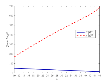
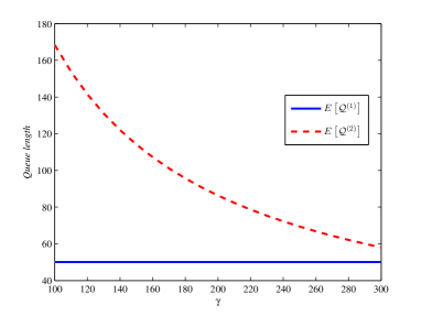
Figure 4: $E\left[\mathcal{Q}^{\left(1\right)}\right]$ and $E\left[\mathcal{Q}^{\left(2\right)}\right]$ vs. $\lambda$ and $\gamma$

(3) The effect of the owner number $N$: We take the parameters: $\lambda=10$, $\mu=0.26$, $\gamma=100$, and $N=43,44,45,\ldots,53$.

Figure 5 shows that $E\left[\mathcal{Q}^{\left(1\right)}\right]$ increases and $E\left[\mathcal{Q}^{\left(2\right)}\right]$ decreases as the owner number $N$ increases. When the owner number $N$ increases, more idle owners are retained in the service platform, while more seekers can receive their services and leave the system immediately. Thus, fewer seekers are kept waiting.

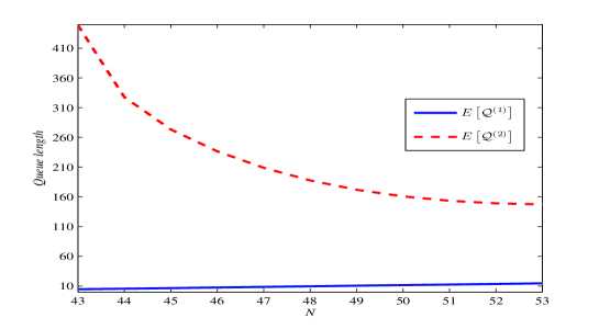
Figure 5: Effect of $N$ on $E\left[\mathcal{Q}^{\left(1\right)}\right]$ and $E\left[\mathcal{Q}^{\left(2\right)}\right]$

(b) The expected profits for the service platform and each owner

(1) The effect of the arrival rate $\lambda$: We take the parameters: $N=60$, $\mu=1$, $\gamma=100$, $P=50$, $d=0.8$ and $\lambda\in\left[10,46\right]$.

The left of Figure 6 that $f_{1}$ and $f_{2}$ increase as the arrival rate $\lambda$ increases. Such numerical results are consistent with our intuitive understanding. As the arrival rate $\lambda$ increases, more seekers enter the system per unit time, which directly improves the expected profits for both the service platform and each owner.

(2) The effect of the service price $P$: We take the parameters: $N=60$, $\lambda=10$, $\mu=1$, $\gamma=100$, $d=0.8$, and $P\in\left[30,50\right]$.

From The right of Figure 4, we show that $f_{1}$ and $f_{2}$ increase as the service price $P$ increases. Clearly, the service platform and each owner earn more with a higher service price $P$.

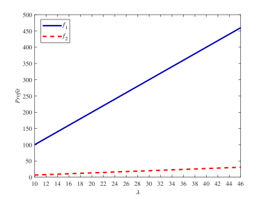
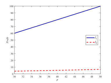
Figure 6: Effect of $\lambda$ and $P$ on $f_{1}$ and $f_{2}$

(c) The expected sojourn time

(1) The effect of the arrival rate $\lambda$: We take the parameters: $N=60$, $\mu=1$, $\gamma=100$, $P=50$, $d=0.8$, and $\lambda\in\left[10,46\right]$.

The left of Figure 7 shows that the expected sojourn time $E\left[W\right]$ increases as the arrival rate $\lambda$ increases. The numerical result is intuitive. With a higher arrival rate, more seekers wait for their services. This leads to a larger expected sojourn time.

(2) The effect of the number of owners $N$: We take the parameters: $\lambda=10$, $\mu=0.26$, $\gamma=100$, $P=50$, $d=0.8$, and $N=43,44,45,\ldots,53$.

The rightt of Figure 7 shows that the expected sojourn time $E\left[W\right]$ decreases as $N$ increases. When the number of owners $N$ increases, the seekers can be more quickly matched with the owners so that the expected sojourn time decreases.

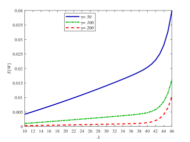
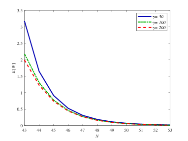
Figure 7: Effect of $\lambda$ and $N$ on $E[W]$

7 Concluding remarks

In this paper, we firstly describe two basic queueing models of service platforms in digital sharing economy according to two different policies of platform matching information: One is at the matching completion time (it is also the service beginning time), while another is at the matching beginning time (no service yet). Then we express the two basic queueing models of service platforms as the level-independent QBD processes, and apply the matrix-geometric method to obtain a necessary and sufficient condition under which the system is stable, the stationary probability vector, the expected sojourn time by using the RG-factorizations, and the expected profits per unit time of a service platform and each owner. This enables performance evaluation of the service platforms. Finally, we use some numerical examples to indicate how the performance measures are influenced by some key system parameters.

We believe that the methodology and results given in this paper are applicable to more extensive queueing analysis of service platforms, and will open a series of promising research, such as in the following directions:

- Extending our basic queueing models to the Markovian arrival process of seekers, and to that one owner can match more than one seekers as a pair.

- Considering several types of owners and/or seekers, and introducing different matching and service priorities, and full-time and part-time owners.

- Based on our two basic queueing models, developing Markov decision processes of service platforms.

- Setting up queueing-game to analyze the owners’ and/or seekers’ strategic behaviors in the study of service platforms and digital sharing economy.

References

- [1] Adan, I., Kleiner, I., Righter, R., & Weiss, G. (2018). FCFS parallel service systems and matching models. Performance Evaluation, 127-128, 253-272.
- [2] Afèhe, P., Liu, Z., & Maglaras, C. (2018). Ride-hailing networks with strategic drivers: The impact of platform control capabilities on performance. Columbia Business School Research Paper, No. 18-19, pp. 1-56.
- [3] Agarwal, N., & Steinmetz, R. (2019). Sharing economy: A systematic literature review. International Journal of Innovation and Technology Management, 16(06), 1930002.
- [4] Akbar, Y. H., & Tracogna, A. (2018). The sharing economy and the future of the hotel industry: Transaction cost theory and platform economics. International Journal of Hospitality Management, 71, 91-101.
- [5] Bai, J., So, K. C., Tang, C. S., Chen, X., & Wang, H. (2019). Coordinating supply and demand on an on-demand service platform with impatient customers. Manufacturing & Service Operations Management, 21(3), 556-570.
- [6] Banerjee, S., Freund, D., & Lykouris, T. (2016). Multi-objective pricing for shared vehicle systems. arXiv preprint arXiv:1608.06819.
- [7] Banerjee, S., Riquelme, C., & Johari, R. (2015). Pricing in ride-share platforms: A queueing-theoretic approach. Available at SSRN: https://ssrn.com/abstract=2568258.
- [8] Bertsimas, D. J., & Van Ryzin, G. (1991). A stochastic and dynamic vehicle routing problem in the Euclidean plane. Operations Research, 39(4), 601-615.
- [9] Bertsimas, D. J., & Van Ryzin, G. (1993). Stochastic and dynamic vehicle routing in the Euclidean plane with multiple capacitated vehicles. Operations Research, 41(1), 60-76.
- [10] Besbes, O., Castro, F., & Lobel, I. (2021). Spatial capacity planning. Operations Research, Published Online: 17 May 2021, https://doi.org/10.1287/opre.2021.2112.
- [11] Braverman, A., Dai, J. G., Liu, X., & Ying, L. (2019). Empty-car routing in ridesharing systems. Operations Research, 67(5), 1437-1452.
- [12] Breidbach, C. F., & Brodie, R. J. (2017). Engagement platforms in the sharing economy: conceptual foundations and research directions. Journal of Service Theory and Practice, 27(4), 761-777.
- [13] Cachon, G. P., Daniels, K. M., & Lobel, R. (2017). The role of surge pricing on a service platform with self-scheduling capacity. Manufacturing & Service Operations Management, 19(3), 368-384.
- [14] Cachon, G. P., & Feldman, P. (2011). Pricing services subject to congestion: Charge per-use fees or sell subscriptions? Manufacturing & Service Operations Management, 13(2), 244-260.
- [15] Castro, F., Nazerzadeh, H., & Yan, C. (2020). Matching queues with reneging: A product form solution. Queueing Systems, 96(3-4), 359-385.
- [16] Chen, M., & Hu, M. (2020). Courier dispatch in on-demand delivery. Available at SSRN: http://ssrn.com/abstract=3675063.
- [17] Cho, S., Park, C., & Kim, J. (2019). Leveraging consumption intention with identity information on sharing economy platforms. Journal of Computer Information Systems, 59(2), 178-187.
- [18] Choi, T. M., Guo, S., Liu, N., & Shi, X. (2019). Values of food leftover sharing platforms in the sharing economy. International Journal of Production Economics, 213, 23-31.
- [19] Choi, T. M., & He, Y. (2019). Peer-to-peer collaborative consumption for fashion products in the sharing economy: Platform operations. Transportation Research Part E: Logistics and Transportation Review, 126, 49-65.
- [20] Chu, L. Y., Wan, Z., & Zhan, D. (2018). Harnessing the double-edged sword via routing: Information provision on ride-hailing platforms. NET Institute Working Paper No. 18-04. Available at SSRN: https://ssrn.com/abstract=3266250.
- [21] Clauss, T., Harengel, P., & Hock, M. (2019). The perception of value of platform-based business models in the sharing economy: Determining the drivers of user loyalty. Review of Managerial Science, 13(3), 605-634.
- [22] Constantiou, I., Marton, A., & Tuunainen, V. K. (2017). Four models of sharing economy platforms. MIS Quarterly Executive, 16(4), 232-251.
- [23] Costello, J. P., & Reczek, R. W. (2020). Providers versus platforms: Marketing communications in the sharing economy. Journal of Marketing, 84(6), 22-38.
- [24] Feng, G., Kong, G., & Wang, Z. (2020). We are on the way: Analysis of on-demand ride-hailing systems. Manufacturing & Service Operations Management, Published Online:3 Jun 2020, https://doi.org/10.1287/msom.2020.0880.
- [25] Feng, Y., Tan, Y. R., Duan, Y., & Bai, Y. (2020). Strategies analysis of luxury fashion rental platform in sharing economy. Transportation Research Part E: Logistics and Transportation Review, 142, 102065.
- [26] Gong, D., Liu, S., Liu, J., & Ren, L. (2020). Who benefits from online financing? A sharing economy E-tailing platform perspective. International Journal of Production Economics, 222, 107490.
- [27] Guo, Y., Li, X., & Zeng, X. (2019). Platform competition in the sharing economy: understanding how ride-hailing services influence new car purchases. Journal of Management Information Systems, 36(4), 1043-1070.
- [28] He, Q. C., Nie, T., Yang, Y., & Shen, Z. J. M. (2019). Beyond rebalancing: Crowd-sourcing and geo-fencing for shared-mobility systems. Available at SSRN: https://ssrn.com/abstract=3293022.
- [29] Hossain, M. (2020). Sharing economy: A comprehensive literature review. International Journal of Hospitality Management, 87, 102470.
- [30] Hu, M. (2020). Spatial or temporal pooling solves wild goose chase. Available at SSRN: http://ssrn.com/abstract=3676065.
- [31] Kim, S. K., & Yeun, C. Y. (2019). A versatile queuing system for sharing economy platform operations. Mathematics, 7(11), 1005.
- [32] Kraus, S., Li, H., Kang, Q., Westhead, P., & Tiberius, V. (2020). The sharing economy: A bibliometric analysis of the state-of-the-art. International Journal of Entrepreneurial Behavior & Research, 26(8), 1769-1786.
- [33] Kung, L. C., & Zhong, G. Y. (2017). The optimal pricing strategy for two-sided platform delivery in the sharing economy. Transportation Research Part E: Logistics and Transportation Review, 101, 1-12.
- [34] Latouche, G., & Ramaswami, V. (1999). Introduction to Matrix Analytic Methods in Stochastic Modeling. SIAM.
- [35] Leoni, G., & Parker, L. D. (2019). Governance and control of sharing economy platforms: Hosting on Airbnb. The British Accounting Review, 51(6), 100814.
- [36] Li, Q. L. (2010). Constructive Computation in Stochastic Models with Applications: The RG-Factorizations. Springer.
- [37] Li, Q. L. & Fan, R. N. (2021). A mean-field matrix-analytic method for bike sharing systems under Markovian environment. Annals of Operations Research, Published Online: 17 June 2021, https://doi.org/10.1007/s10479-021-04140-x.
- [38] Liu, H. L., Li, Q. L., Chang, Y. X., & Zhang, C. (2020). Block-structured double-ended queues and bilateral QBD processes. arXiv preprint arXiv:2001.00946.
- [39] Liu, H. L., Li, Q. L., & Zhang, C. (2020). Matched queues with matching batch pair . arXiv preprint arXiv:2009.02742.
- [40] Narasimhan, C., Papatla, P., Jiang, B., et al. (2018). Sharing economy: Review of current research and future directions. Customer Needs and Solutions, 5(1), 93-106.
- [41] Neuts, M. F. (1981). Matrix-Geometric Solutions in Stochastic Models: An Algorithmic Approach. Johns Hopkins University Press.
- [42] Serfozo, R. (1999). Introduction to Stochastic Networks. Springer-Verlag.
- [43] Sun, L., Teunter, R. H., Hua, G., & Wu, T. (2020). Taxi-hailing platforms: Inform or Assign drivers? Transportation Research Part B: Methodological, 142, 197-212.
- [44] Sutherland, W., & Jarrahi, M. H. (2018). The sharing economy and digital platforms: A review and research agenda. International Journal of Information Management, 43, 328-341.
- [45] Taylor, T. A. (2018). On-demand service slatforms. Manufacturing & Service Operations Management, 20(4), 704-720.
- [46] Wang, L., & Yan, X. (2019). New taxi–passenger dispatching model at terminal station. Journal of Transportation Engineering, Part A: Systems, 145(7), 04019026.
- [47] Weiss G (2020). Directed FCFS infinite bipartite matching. Queueing Systems, 96, 387–418.
- [48] Wen, X., & Siqin, T. (2020). How do product quality uncertainties affect the sharing economy platforms with risk considerations? A mean-variance analysis. International Journal of Production Economics, 224, 107544.
- [49] Wirtz, J., So, K. K. F., Mody, M. A., Liu, S. Q., & Chun, H. H. (2019). Platforms in the peer-to-peer sharing economy. Journal of Service Management, 30(4), 452-483.
- [50] Xu, X., Zeng, S., & He, Y. (2021). The impact of information disclosure on consumer purchase behavior on sharing economy platform Airbnb. International Journal of Production Economics, 231, 107846.
- [51] Zhong, Y., Wan, Z., & Shen, Z. J. M. (2019). Balancing supply and demand: Queuing vs. surge pricing mechanisms. Working paper, University of Chicago, IL.