Abstract: The Riemann hypothesis states that the Riemann $\xi(s)$ function has no zeros in the strip $0<{\rm Re}(s)<1$ except for the critical line where ${\rm Re}(s)=1/2$. However, determining whether a point in the strip is a zero of a complex function is a challenging task. Bombieri proposed an assertion in the Official Problem Description that states, “The Riemann hypothesis is equivalent to the statement that all local maxima of $\xi(t)$ (namely $\xi(s)$ on the critical line) are positive and all local minima are negative.” In this paper, we follow Bombieri’s idea to study the Riemann hypothesis. First, we show that on the critical line, the $\xi(s)$ function (which is then a real function of a single real variable) obeys a special differential equation, such that it satisfies Bombieri’s equivalence condition. Then, since we have been unable to locate the original proof of Bombieri’s equivalence theorem, we independently provide a proof for the sufficiency part of it. Namely, if the $\xi(s)$ function satisfies Bombieri’s equivalence condition on the critical line, then by the Cauchy-Riemann equations, it has no zeros outside this critical line. Thus, we can conclude that the Riemann hypothesis is true. Finally, we comment on Pólya’s counterexample against using the simplified $\xi(s)$ function to study the Riemann hypothesis, noting that it violates Bombieri’s equivalence theorem.

Key Words: Riemann hypothesis.

1. Introduction

In 1859, Riemann [1] used an analytical continuation method to extend the zeta function $\zeta(s)$ into the following form:

$$\xi(s)=\frac{1}{2}s(s-1)\pi^{-s/2}\Gamma\Big{(}\frac{s}{2}\Big{)}\zeta(s),$$ (1)

where, the function $\xi(s)$ can be analytically expressed as

$$\xi(s) = \frac{1}{2}+\frac{1}{2}s(s-1)\int\limits_{1}^{\infty}\Psi(\tau)\Big{(}\tau^{s/2-1}+\tau^{-(1+s)/2}\Big{)}{\rm d}\tau,$$

$$\Psi(\tau) = \sum\limits_{n=1}^{\infty}e^{-\pi n^{2}\tau}=\frac{1}{2}\Big{(}\theta(\tau)-1\Big{)},$$ (2)

$\theta(\tau)$ is the third Jacobian theta function. Riemann stated that every zero of the function $\xi(s)$, which is also the non-trivial zero of the zeta function $\zeta(s)$, is located on the critical strip $0\leq{\rm Re}(s)\leq 1$. Then, he asserted that all zeros are most likely to lie on the line ${\rm Re}(s)=1/2$. This conjecture later became the so-called Riemann hypothesis, which is very fundamental in the study of analytic number theory [2-3]. Due to its importance, the Riemann hypothesis was proposed as one of the famous Hilbert problems in 1900, specifically as number eight out of twenty-three. In 2000, it was selected again as one of the seven Clay Millennium Prize Problems [4-5].

The Riemann hypothesis can also be expressed as the statement that the function $\xi(s)$ has no zeros on the entire strip except for the critical line where ${\rm Re}(s)=1/2$. However, determining whether a point on the strip is a zero of a complex function is a challenging task. Research in this direction has made very little progress so far. In 1896, Hadamard [6] and de la Vallée Poussin [7] independently proved that there are no zeros on the two boundaries ${\rm Re}(s)=0$ and ${\rm Re}(s)=1$, and with this result, they also proved the prime number theorem. Bohr and Landau [8] showed in 1914 that almost all zeros are located inside a small $\varepsilon$-domain attached to the critical line. Certainly, the phrase “almost all” allows for some exceptional zeros outside of this domain.

Bombieri proposed an assertion in the Official Problem Description [4] that states, “The Riemann hypothesis is equivalent to the statement that all local maxima of $\xi(t)$ (namely $s=1/2+{\rm i}t$ in the above equation) are positive and all local minima are negative.” If this claim is true, it would open up a better way to study the Riemann hypothesis. On the critical line, the $\xi(s)$ function becomes a real function of a single real variable, which has a relatively simpler curve geometry compared to the complex $\xi(s)$ function in the strip, and can be handled by more advanced mathematical tools. So far, we know that Hardy [9] proved that $\xi(s)$ has infinitely many zeros on the critical line, and several authors such as Platt and Trudgian [10] have numerically shown that the Riemann hypothesis holds up to ${\rm Im}(s)\leq 3\cdot 10^{12}$.

We will follow Bombieri’s idea to study the Riemann hypothesis.

First, in Section 2, we simplify the complicated $\xi(s)$ function using Jensen’s method. We use some different notations in the formulas compared to other authors to provide the best viewpoint for studying the Riemann hypothesis in the following sections. We then list several important properties of the Jensen function that are necessary for handling the $\xi(s)$ function on the critical line.

In Section 3, we show that on the critical line, the $\xi(s)$ function (which is then a real function of a single real variable) obeys a special differential equation. As a consequence, the function must have a curve geometry that increases and is concave downward (or decreases and is concave upward) around a zero. This ensures that all zeros of the function are simple zeros, all local maxima are greater than zero, and all local minima are less than zero. Therefore, the function satisfies the Bombieri equivalence condition.

Furthermore, in Section 4, since we have been unable to locate the original proof of Bombieri’s equivalence theorem, we will independently provide a proof for the sufficiency part of it. We show that if the $\xi(s)$ function satisfies Bombieri’s equivalence condition on the critical line, then by the Cauchy-Riemann equations, it has no zeros outside this critical line. Thus, we can conclude that the Riemann hypothesis is true.

Finally, in Section 5, since Pólya had a counterexample against using Jensen’s form of the $\xi(s)$ function to study the Riemann hypothesis, we comment on the counterexample for its violation of Bombieri’s equivalence theorem. Therefore, Pólya’s counterexample does not contradict this work.

2. Simplified $\xi$-function and properties of Jensen’s function

First, we briefly review the simplified formula of Riemann’s $\xi(s)$ function. The formula was originally created by Riemann in his paper [1] before he put forth the hypothesis. In the 1911 Copenhagen conference [11], Jensen put the formula into an elegant form of a Fourier cosine transform. This formula was later used by subsequent authors such as Titchmarsh [12], Wintner [13], Haviland [14], Spira [15], Matiyasevich [16], Pólya [17], and many others.

We need to change some notations in the formula. This will benefit us in handling the $\xi(s)$ function by applying basic calculus, such as differential equations and Cauchy-Riemann equations. Starting with (1. Introduction), we introduce a new complex variable $z\in\mathbb{C}$ as $z=x+{\rm i}y$ to make a transformation,

$$s=\frac{1}{2}(z+1).$$ (3)

Then, $\xi(s)$ is rewritten as follows

$$\xi(s)=\Xi(z)=\frac{1}{2}+\frac{1}{8}\big{(}z^{2}-1\big{)}\int\limits_{1}^{\infty}\Psi(\tau)\tau^{-3/4}\big{(}\tau^{z/4}+\tau^{-z/4}\big{)}{\rm d}\tau.$$ (4)

This notation $\Xi(z)$ is different from that of Jensen [11,18] and Landau [19], who took (3) as $s=1/2+{\rm i}z$. By using (3), the concerned strip $0<{\rm Re}(s)<1$ to search for the zeros of the function $\xi(s)$ in the $s$-plane has been changed to $-1<{\rm Re}(z)<1$ in the $z$-plane for the function $\Xi(z)$. The critical line ${\rm Re}(s)=1/2$ becomes ${\rm Re}(z)=x=0$.

Furthermore, we change the integral argument to $t$ by

$$\tau=e^{4t},$$ (5)

thus,

$$\Xi(z)=\frac{1}{2}+\frac{1}{2}\big{(}z^{2}-1\big{)}\int\limits_{0}^{\infty}\Psi(e^{4t})e^{t}\big{(}e^{zt}+e^{-zt}\big{)}{\rm d}t.$$ (6)

Using a hyperbolic function $\cosh(w)=(e^{w}+e^{-w})/2$, we have

$$\Xi(z)=\frac{1}{2}+\big{(}z^{2}-1\big{)}\int\limits_{0}^{\infty}F(t)\cosh(zt){\rm d}t,$$ (7)

where,

$$F(t)=\Psi(e^{4t})e^{t}=\sum\limits_{n=1}^{\infty}\exp\big{(}t-\pi n^{2}e^{4t}\big{)}.$$ (8)

Now we will continue working on the function $F(t)$. Taking the first and second order differentials, we obtain:

$$F^{\prime}(t)=\sum\limits_{n=1}^{\infty}\exp\big{(}t-\pi n^{2}e^{4t}\big{)}\;\big{(}1-4\pi n^{2}e^{4t}\big{)},$$ (9)

$$F^{\prime\prime}(t) = \sum\limits_{n=1}^{\infty}\exp\big{(}t-\pi n^{2}e^{4t}\big{)}\;\Big{[}\big{(}1-4\pi n^{2}e^{4t}\big{)}^{2}-16\pi n^{2}e^{4t}\Big{]}$$ (10)

$$= F(t)+G(t),$$

where

$$G(t)=\sum\limits_{n=1}^{\infty}\exp\big{(}t-\pi n^{2}e^{4t}\big{)}\;\Big{[}16\pi^{2}n^{4}e^{8t}-24\pi n^{2}e^{4t}\Big{]}$$ (11)

is called Jensen function [11], which is different from Jensen’s original formula by a constant factor of 8. At $t=0$, we have [20]

$$F(0)=\sum\limits_{n=1}^{\infty}\exp\big{(}-\pi n^{2}\big{)}=\frac{1}{2}\big{(}\theta(1)-1\big{)},$$ (12)

$$F^{\prime}(0)=\sum\limits_{n=1}^{\infty}\exp\big{(}-\pi n^{2}\big{)}\;\big{(}1-4\pi n^{2}\big{)}=-\frac{1}{2},$$ (13)

and at $t\to\infty$,

$$\lim\limits_{t\to\infty}F(t)\sinh(zt)=0,\hskip 22.76219pt\lim\limits_{t\to\infty}F^{\prime}(t)\cosh(zt)=0,$$ (14)

where the theta function $\theta(1)$ in (12) is a finite value that can be obtained from Whittaker and Watson [21], while (13) and (14) should have originally been found by Riemann [1] because they are indispensable for working with the integral representation of the $\xi(s)$ function. With these preparations, we can further simplify (7). By using integration by parts,

$$\int\limits_{0}^{\infty}F(t)\,\cosh(zt){\rm d}t = \frac{1}{z^{2}}F^{\prime}(0)+\frac{1}{z^{2}}\int\limits_{0}^{\infty}[F(t)+G(t)]\,\cosh(zt){\rm d}t.$$ (15)

Thus,

$$(z^{2}-1)\int\limits_{0}^{\infty}F(t)\,\cosh(zt){\rm d}t\ =\ F^{\prime}(0)+\int\limits_{0}^{\infty}G(t)\,\cosh(zt){\rm d}t.$$ (16)

Substituting (16) into (7), we obtain an integral representation form of the Riemann’s $\xi(s)$ function, which we call the simplified $\xi(s)$ function in this paper [20]:

$$\Xi(z)=\int\limits_{0}^{\infty}G(t)\,\cosh(zt){\rm d}t.$$ (17)

Now, we review several properties of the Jensen function. It is easy to check that the Jensen function $G(t)>0$ on $0<t<\infty$, and $G(t)\to 0$ very fast when $t\to\infty$. In a two-page note, Wintner [13] proved that $G(t)$ is strictly decreasing, i.e., $G^{\prime}(t)<0$. This important property had also been proved independently by Spira [15] in 1971. In his note, Wintner pointed out a property crediting to Jensen, Hurwitz and others: if the definition domain of $G(t)$ is extended to the negative $t$-axis, it is also an even function, i.e., $G(-t)=G(t)$, and $G^{\prime}(0)=0$. Since it is not easy to see this property from (11), we briefly repeat the proof as follows. Recall (8),

$$F(t)=\Psi(\tau)e^{t},\hskip 14.22636pt\tau(t)=e^{4t},\hskip 14.22636pt\tau^{\prime}(t)=4\tau(t),\hskip 14.22636pt\tau(-t)=\frac{\ 1\ }{\tau(t)},$$ (18)

we can calculate

$$G(t)=F^{\prime\prime}(t)-F(t)=\Big{[}16\tau^{2}\Psi^{\prime\prime}(\tau)+24\tau\Psi^{\prime}(\tau)\Big{]}e^{t}.$$ (19)

Applying derivatives to the identity of Jacobi that Riemann gave in his paper [1]

$$2\Psi(\tau)+1=\tau^{-1/2}\Big{[}2\Psi\Big{(}\frac{1}{\tau}\Big{)}+1\Big{]},$$ (20)

we obtain

$$\Big{[}16\tau^{2}\Psi^{\prime\prime}(\tau)+24\tau\Psi^{\prime}(\tau)\Big{]}e^{t}=\Big{[}\frac{\ 16\ }{\tau^{2}}\Psi^{\prime\prime}\Big{(}\frac{1}{\tau}\Big{)}+\frac{\ 24\ }{\tau}\Psi^{\prime}\Big{(}\frac{1}{\tau}\Big{)}\Big{]}e^{-t}=G(-t).$$ (21)

Thus, $G(t)$ is analogous to a Gaussian function. Its bell-shaped curve [20] is shown in Figure 1. This feature has motivated many researchers to create other similar $G(t)$ functions to study the Riemann hypothesis. For example, see [17].

....................................................................................................................................................................................................................................................................................................................................................................................................................................................................................................................................................................................................................................................................................................................................................................................................................................................................................................................................................................................................................................................................................................................................................................................................................................................................................................................................................................................................................................................................................................................................................................................................................................................................................................................................................................................................................................................................................................................................................................................................................................................................................................................................................................................................................................................................................................................................................................................................................................................................................................................................................................................................................................................................................................................................................................................................................................................                                                                                                                                                                                                              $$-0.5 -0.4 -0.3 -0.2 -0.1 t G(t)$$0.00.10.20.30.40.5                 1.02.03.0

Figure 1: The curve shape of function $G(t)$.

Since $G(t)$ is a smooth (infinitely differentiable) even function, Jensen [18] showed that its derivatives of any order at $t=0$ and $\infty$ are given by

$$G^{(2k-1)}(0)=0,\hskip 28.45274ptG^{(2k)}(0)={\rm exists},\hskip 28.45274pt\lim\limits_{t\to\infty}G^{(k)}(t)=0.$$ (22)

Although Jensen did not give a formula for even order derivatives, it is shown from (1. Introduction) and (19) that $G^{(2k)}(0)$ is related to $\theta^{(2k+2)}(1),\ \theta^{(2k+1)}(1),\ \cdots,\ \theta^{\prime}(1)$. In recent years, Romik [22] found a formula to calculate all derivatives of the $\theta(\tau)$ function at $\tau=1$. Using Romik’s formula, we have calculated [20]

$$G(0)\approx 3.5736,\hskip 14.22636ptG^{\prime\prime}(0)\approx-267.6880,\hskip 14.22636ptG^{(4)}(0)\approx 51978.4213,\ \cdots.$$ (23)

Jensen [18] also discovered many other properties of $G(t)$ and its derivatives, which have been well summarized by Gélinas [23]. In his reading notes, Gélinas has also extended more interesting equations for the $G(t)$ function. For example, for $t\geq 0$,

$$(2\pi\tau-3)\pi\tau e^{t-\pi\tau}\ <\ \frac{1}{8}G(t)\ <\ (2\pi\tau-3)\pi\tau e^{t-\pi\tau}+32\pi^{2}\tau^{2}e^{t-4\pi\tau},$$ (24)

and

$$4G(t)\ <\ \frac{\ -G^{\prime}(t)\ }{\pi\tau-\pi}\ <\ 4G(t)+8(8\pi-18)\pi\tau e^{t-\pi\tau}.$$ (25)

These two inequalities will play important roles in the following work.

We will use (17) to study the Riemann hypothesis. Let $z=x+{\rm i}y$. The function $\Xi(z)$ can be divided into its real and imaginary parts as follows:

$$\Xi(z) = u(x,y)+{\rm i}\;\!v(x,y)$$ (26)

$$= \int\limits_{0}^{\infty}G(t)\cosh(xt)\cos(yt){\rm d}t+{\rm i}\int\limits_{0}^{\infty}G(t)\sinh(xt)\sin(yt){\rm d}t,$$

Therefore, $\Xi(z)=0$ is equivalent to $u(x,y)=v(x,y)=0$.

3. Bombieri’s equivalence condition

As mentioned in the introduction, we will follow Bombieri’s equivalence theorem to study the Riemann hypothesis. In this section, we focus our attention on the critical line, namely $x=0$, where the $\Xi(z)$ function becomes a real function of a single real variable:

$$u(0,y) = \Xi({\rm i}y)=\int\limits_{0}^{\infty}G(t)\cos(yt){\rm d}t=:U(y),$$

$$v(0,y) = 0.$$ (27)

We will demonstrate that the function satisfies Bombieri’s equivalence condition.

Lemma 1. For sufficient large $y$, the $k$-th derivative of $U(y)$ satisfies the following asymptotic equation,

$$U^{(k)}(y)=(-1)^{k}\Big{(}\frac{\pi}{8}-\frac{1}{4y}\Big{)}^{k}U(y)\Big{(}1+{\mathcal{O}}(y^{-1})\Big{)}.$$ (28)

Proof. According to Titchmarsh [24], when the modulus of $s$ is sufficient large, the $\xi(s)$ function behaves asymptotically as

$$\log\xi(s)=\frac{1}{2}s\log{s}+{\mathcal{O}}(1).$$ (29)

Thus, we set $s=(1+{\rm i}y)/2$ into (29), where $y$ is sufficient large,

$$\log U(y) = \log\xi\Big{(}\frac{1+{\rm i}y}{2}\Big{)}=-\frac{y}{4}\arctan\Big{(}\frac{y}{1}\Big{)}+\frac{1}{4}\log\sqrt{1+y^{2}}+{\mathcal{O}}(1)$$ (30)

$$= -\frac{\pi}{8}y+\frac{1}{4}\log y+{\mathcal{O}}(y^{-1}).$$

Differentiating $U(y)$, we have

$$U^{\prime}(y)=-\Big{(}\frac{\pi}{8}-\frac{1}{4y}\Big{)}U(y)\Big{(}1+{\mathcal{O}}(y^{-1})\Big{)}.$$ (31)

Continuing to differentiate this equation for several times, we get (28). $\square$

Remark. Titchmarsh gave the order estimation (29) through an analysis of (1), in which he ignored the term $s(s-1)$. If this term is added back to (29) we get

$$\log\xi(s)=\frac{1}{2}s\log{s}+2\log{s}+{\mathcal{O}}(1).$$ (32)

Then, by a similar work (28) will be adjusted as

$$U^{(k)}(y)=(-1)^{k}\Big{(}\frac{\pi}{8}-\frac{9}{4y}\Big{)}^{k}U(y)\Big{(}1+{\mathcal{O}}(y^{-1})\Big{)}.$$ (33)

As we will see, this adjustment has no impact on the proof of Lemma 2 below.

Lemma 2. All zeros of the function $U(y)$ in (3. Bombieri’s equivalence condition) are simple zeros.

Proof. Assume that $U(y)$ has a zero $y_{0}$ of order $n$. We can express $U(y)$ as a Taylor series expansion around $y_{0}$ and obtain $U(y)\approx U^{(n)}(y_{0})(y-y_{0})^{n}/n!$, where $U^{(n)}(y_{0})\neq 0$. Thus, in the interval $y_{0}<y<y_{0}+\delta$, for sufficiently small $\delta>0$, if $U(y)>0$, then all derivatives $U^{(k)}(y)>0$ for $1\leq k\leq n$. We need to show that this is not possible for $n\geq 2$.

We differentiate $U(y)$ in (3. Bombieri’s equivalence condition), and then integrate by parts to get

$$yU^{\prime}(y)+U(y)=-\int\limits_{0}^{\infty}G^{\prime}(t)t\cos(yt)\;\!{\rm d}t.$$ (34)

We differentiate $U(y)$ again to obtain the second-order derivative,

$$U^{\prime\prime}(y)=-\int\limits_{0}^{\infty}G(t)t^{2}\cos(yt)\;\!{\rm d}t.$$ (35)

These two equations motivate us to establish a relationship between $G^{\prime}(t)t$ and $G(t)t^{2}$. Using the left-hand inequality in (24), we have

$$\pi\tau e^{t-\pi\tau}<\frac{1}{\ 8(2\pi\tau-3)\ }G(t),$$ (36)

which is substituted into the right-hand inequality in (25) to obtain

$$4G(t)<\frac{\ -G^{\prime}(t)\ }{\pi\tau-\pi}<4G(t)+\frac{\ 8\pi-18\ }{2\pi\tau-3}G(t).$$ (37)

Since $\tau=e^{4t}=1+4t+\cdots$, we rearrange (37) as

$$16\pi\;\!G(t)<-\frac{G^{\prime}(t)}{t}<16\pi\frac{(e^{4t}-1)}{4t}\bigg{[}1+\frac{\ 4\pi-9\ }{4\pi e^{4t}-6}\bigg{]}G(t).$$ (38)

This equation implies that $-G^{\prime}(t)/t$ is at least $16\pi$ times greater than $G(t)$. Figure 2 (obtained from [20]) shows a comparison of the three curves, which also validates (24) and (25).

.....................................................................................................................................................................................................................................................................................................................................................................................................................................................................................................................................................................$$\frac{e^{4t}-1}{4t}\bigg{[}1+\frac{\ 4\pi-9\ }{4\pi e^{4t}-6}\bigg{]}G(t) -\frac{1}{16\pi t}G^{\prime}(t) G(t) t$$........................................................................................................................................................................................................................................................................................................................................................................................................................................................................................................................................................................................................................................................................................................................................................................................................................................................................................................................................................................................................................................................................................................................................................................................................................................................................................................................................................................................................................................................................................................................................................................................................................................................................................................................................................................................................................................................................................................................................                        0.00.10.20.30.40.5                           1.02.03.04.05.06.0

Figure 2: The relation between functions $-G^{\prime}(t)/t$ and $G(t)$.

We assume that the ratio of $-G^{\prime}(t)/t$ to $G(t)$ can be expressed as a function of $a(t)$. As both $G(t)$ and $-G^{\prime}(t)/t$ are even functions, $a(t)$ is also even. We can express $a(t)$ as a series:

$$a(t)=\frac{-G^{\prime}(t)}{t\;\!G(t)}=a_{0}+a_{2}t^{2}+a_{4}t^{4}+a_{6}t^{6}+\cdots.$$ (39)

By setting $t=0$ in (39), we obtain the value of $a_{0}$ as [20]:

$$a_{0}=\lim\limits_{t\to 0}\frac{-G^{\prime}(t)}{\ tG(t)\ }=-\frac{G^{\prime\prime}(0)}{G(0)}\approx 1.4902\times 16\pi\approx 74.9076>0.$$ (40)

Using $G(0)$, $G^{\prime\prime}(0)$, and $G^{(4)}(0)$ in (23), the value $a_{2}$ is also calculated [20]:

$$a_{2} = \lim\limits_{t\to 0}\frac{1}{t^{2}}\Big{(}-\frac{G^{\prime}(t)}{tG(t)}-a_{0}\Big{)}=\frac{3[G^{\prime\prime}(0)]^{2}-G(0)G^{(4)}(0)}{6[G(0)]^{2}}$$ (41)

$$\approx 381.3732=5.0912a_{0}.$$

Although we can continue this process to determine other coefficients, the calculation becomes very tedious. However, we can use an approximate set of coefficients $\{a_{2k}\}$ for the relation between $G^{\prime}(t)t$ and $G(t)t^{2}$, as long as the resulting series (39) is close enough to the $a(t)$ function.

....................................................................................................................................................................................................................................................................................................................................................................................................................................................................................................................................................$$a_{0}\cosh(4t) a(t) a_{0}\sinh(4t)/(4t) t \frac{\ a(t)\ }{16\pi}$$..................................................................................................................................................................................................................................................................................................................................................................................................................................................................................................................................................................................................................................................................................................................................................................................................................................................................................................................................................................................................................................................................................................................................................................................................................................................................................................................................................................................................................................................................................................................................................................................................................................................................................................................................................................................................................................................................................................................................................................................................................................................................................................................................................................................................................................................................................................................................................................................................................................................................................................................................................................................................................................Fitted                         0.00.20.40.60.81.0                                       051015

Figure 3: The curve plots of $a(t)$ and the two bounded functions.

From (37) or Figure 2, we know that there exists a smooth function $b(t)\approx 1$ such that

$$a(t)=\frac{-G^{\prime}(t)}{t\;\!G(t)}=16\pi\bigg{[}1+b(t)\frac{\ 4\pi-9\ }{4\pi e^{4t}-6}\bigg{]}\frac{(e^{4t}-1)}{4t},$$ (42)

where $b(0)<b(t)<1$, and $b(0)\approx 0.9026$ can be calculated [20] from $a_{0}$ by

$$a_{0}=16\pi\bigg{[}1+b(0)\frac{\ 4\pi-9\ }{4\pi-6}\bigg{]}.$$ (43)

From (42), $a(t)$ is dominated by $(e^{4t}-1)/(4t)$, which has two even asymptotic functions: $\sinh(4t)/(4t)$ and $\cosh(4t)$. We can then easily verify that

$$a_{0}\frac{\sinh(4t)}{4t}\leq a(t)\leq a_{0}\cosh(4t),$$ (44)

as shown by the curve plots in Figure 3 (obtained in [20]). Thus, taking Taylor expansions for $\sinh(4t)/(4t)$ and $\cosh(4t)$, respectively, and using (39) for $a(t)$, we have

$$a_{0}\sum\limits_{k=0}^{\infty}\frac{4^{2k}}{(2k+1)!}t^{2k}\leq\sum\limits_{k=0}^{\infty}a_{2k}t^{2k}\leq a_{0}\sum\limits_{k=0}^{\infty}\frac{4^{2k}}{(2k)!}t^{2k}.$$ (45)

The three series in (45) have a common starting value $a_{0}$ at $t=0$, and the curvature of $a(t)$ (i.e., from (41), $a_{2}=5.0912a_{0}$) is between the other two: $(8/3)a_{0}<a_{2}<8a_{0}$. When $t\to\infty$, according to (42) and (45),

$$\lim\limits_{t\to\infty}\frac{a(t)}{a_{0}\sinh(4t)/(4t)} = \Big{(}\sum\limits_{k=0}^{\infty}a_{2k}\Big{)}\Big{(}a_{0}\sum\limits_{k=0}^{\infty}\frac{4^{2k}}{(2k+1)!}\Big{)}^{-1}=\frac{32\pi}{a_{0}},$$

$$\lim\limits_{t\to\infty}\frac{a(t)}{a_{0}\cosh(4t)} = 0,$$ (46)

This means that $a_{2k}$ approaches rapidly to $a_{0}4^{2k}/(2k+1)!$ as $k$ increases. These properties allow $a_{2k}$ to be well approximated by a weighted average of the other two sequences,

$$a_{2k}=(1-c_{2k})a_{0}\frac{4^{2k}}{(2k+1)!}+c_{2k}a_{0}\frac{4^{2k}}{(2k)!},\hskip 14.22636pt(k=0,1,2,\cdots),$$ (47)

where we restrict $-1/(2k)<c_{2k}\leq 1$ such that $0<a_{2k}\leq a_{0}4^{2k}/(2k)!$. For example, we [20] have manually created a set of $a_{2k}$ as shown in Table 1. The resulting fitted curve is also plotted in Figure 3 for comparison. The fitting error is denoted by

$$\Delta=\max\limits_{0\leq t<\infty}\Bigg{|}a(t)\Big{(}\sum\limits_{k=0}^{\infty}a_{2k}t^{2k}\Big{)}^{-1}-1\Bigg{|}.$$ (48)

According to equation (3. Bombieri’s equivalence condition), the larger the index of $k$, the more accurate $a_{2k}$ will be. Thus, fitting errors are due to the terms with small $k$, which means that errors occur in the small $t$ region. For our example [20], we have $\Delta\leq 0.008$. However, one can obtain a smaller $\Delta$ using an optimization method.

Table 1: A calculation example of coefficients $a_{2k}$.

$2k$	2	4	6	8	10	$\geq 12$
$c_{2k}$	0.351	-0.095	0.21	0.1	0.01	0
$a_{2k}/a_{0}$	4.5387	1.3227	1.8367	0.3251	0.0289	$4^{2k}/(2k+1)!$
$a_{2k}/a_{0}\cdot(\pi/8)^{2k}$	0.6999	0.0315	0.0067	0.0002	0.0000	0.0000

Using the function $a(t)$ and the equation $-G^{\prime}(t)\;\!t=G(t)\;\!t^{2}\;\!a(t),$ we can combine $U(y),$ $U^{\prime}(y),$ and $U^{\prime\prime}(y)$ together. Referring to equations (34) and (48), we have

$$yU^{\prime}(y)+U(y) = -\int\limits_{0}^{\infty}G^{\prime}(t)t\cos(yt)\;\!{\rm d}t=\int\limits_{0}^{\infty}G(t)\;\!t^{2}\;\!a(t)\cos(yt)\;\!{\rm d}t$$ (49)

$$= \int\limits_{0}^{\infty}G(t)\;\!t^{2}\;\!a(t)\Big{(}\sum\limits_{k=0}^{\infty}a_{2k}t^{2k}\Big{)}^{-1}\Big{(}\sum\limits_{k=0}^{\infty}a_{2k}t^{2k}\Big{)}\cos(yt)\;\!{\rm d}t$$

$$= A\int\limits_{0}^{\infty}G(t)\Big{(}a_{0}t^{2}+a_{2}t^{4}+a_{4}t^{6}+a_{6}t^{8}+\cdots\Big{)}\cos(yt)\;\!{\rm d}t,$$

where $A$ denotes a parameter that varies in a very narrow region $(1-\Delta<A<1+\Delta)$, and has been treated as a constant and taken out from the integral. By differentiating (35) further for the higher order derivatives, we obtain

$$U^{(2k)}(y)=(-1)^{k}\int\limits_{0}^{\infty}G(t)t^{2k}\cos(yt)\;\!{\rm d}t,$$ (50)

which we can use to rewrite the previous equation as

$$yU^{\prime}(y)+U(y)\ =-A\Big{[}a_{0}U^{\prime\prime}(y)-a_{2}U^{(4)}(y)+a_{4}U^{(6)}(y)-a_{6}U^{(8)}(y)+\cdots\Big{]}.$$ (51)

According to Hardy [9], $U(y)$ has infinitely many zeros on $0<y<\infty$. Let $y_{0}$ be one such zero. We assume $y_{0}$ is sufficiently large because Platt and Trudgian [10,20] have already shown that the zeros up to $y\leq 6\cdot 10^{12}$ are simple. Let’s assume that $y_{0}$ is a zero of order 2. Then, in the neighborhood of $y_{0}$, $U(y)$ can be expressed as

$$U(y)=\frac{1}{2}U^{\prime\prime}(y_{0})(y-y_{0})^{2}\Big{(}1+{\mathcal{O}}(y-y_{0})\Big{)},$$ (52)

where $U^{\prime\prime}(y_{0})\not=0$. Thus, in this neighborhood, $U^{\prime\prime}(y)\not=0$. Since $y$ is large, according to Lemma 1, we have

$$U^{(2k+2)}(y)=\Big{(}\frac{\pi}{8}-\frac{1}{4y}\Big{)}^{2k}U^{\prime\prime}(y)\Big{(}1+{\mathcal{O}}(y^{-1})\Big{)},\hskip 14.22636pt(k=1,2,3,\cdots).$$ (53)

We substitute (53) into (51) and get

$$yU^{\prime}(y)+U(y)\ =\ -Ac\,U^{\prime\prime}(y)+{\mathcal{O}}\Big{(}\frac{U^{\prime\prime}(y)}{y}\Big{)},$$ (54)

where

$$c=a_{0}-a_{2}\Big{(}\frac{\pi}{8}-\frac{1}{4y}\Big{)}^{2}+a_{4}\Big{(}\frac{\pi}{8}-\frac{1}{4y}\Big{)}^{4}-a_{6}\Big{(}\frac{\pi}{8}-\frac{1}{4y}\Big{)}^{6}+\cdots.$$ (55)

It is seen that (55) is an alternating series. According to (47), if $0\leq c_{2k}\leq 1$, we have

$$a_{0}\frac{4^{2k}}{(2k+1)!}\leq a_{2k}\leq a_{0}\frac{4^{2k}}{(2k)!},\hskip 14.22636pt(k=0,1,2,\cdots).$$ (56)

Thus, the series satisfies the conditions of Leibniz’ theorem:

$$a_{2}\Big{(}\frac{\pi}{8}-\frac{1}{4y}\Big{)}^{2} \leq 4.5387a_{0}\Big{(}\frac{\pi}{8}\Big{)}^{2}\ <\ a_{0},$$ (57)

$$a_{2k+2}\Big{(}\frac{\pi}{8}-\frac{1}{4y}\Big{)}^{2k+2} \leq a_{0}\frac{4^{2k+2}}{(2k+2)!}\Big{(}\frac{\pi}{8}-\frac{1}{4y}\Big{)}^{2k+2}$$ (58)

$$\leq a_{0}\frac{4^{2k}}{(2k+1)!}\Big{(}\frac{\pi}{8}-\frac{1}{4y}\Big{)}^{2k}\frac{1}{2k+2}\Big{(}\frac{\pi}{2}\Big{)}^{2}$$

$$\leq a_{2k}\Big{(}\frac{\pi}{8}-\frac{1}{4y}\Big{)}^{2k},\hskip 28.45274pt(k=1,2,3,\cdots),$$

and

$$\lim\limits_{k\to\infty}a_{2k}\Big{(}\frac{\pi}{8}-\frac{1}{4y}\Big{)}^{2k} \leq \lim\limits_{k\to\infty}a_{0}\frac{4^{2k}}{(2k)!}\Big{(}\frac{\pi}{8}\Big{)}^{2k}\ =\ 0.$$ (59)

If $-1/(2k)<c_{2k}\leq 0$, due to the factor of $(\pi/8)$ in the series (55), one can check that $a_{2k}$ still satisfies the Leibniz conditions. The $c_{4}$ of the previous example belongs to this case, which has been shown in Table 1. Thus, the series (55) converges and the value

$$a_{0}-a_{2}\Big{(}\frac{\pi}{8}-\frac{1}{4y}\Big{)}^{2}\leq c\leq a_{0}.$$ (60)

From (57), we have $c>0$, consequently, $Ac>0$.

Therefore, for $y=y_{0}+\delta$, where $\delta>0$ is sufficiently small, according to (52), if $U(y)>0$, then we have $U^{\prime}(y)>0$ and $U^{\prime\prime}(y)>0$. Otherwise, if $U(y)<0$, then we have $U^{\prime}(y)<0$ and $U^{\prime\prime}(y)<0$. However, both of these cases contradict (54).

Let’s assume that $y_{0}$ is a zero of order 3. We differentiate equation (51) with respect to $y$,

$$yU^{\prime\prime}(y)+2U^{\prime}(y)\ =\ -A\Big{[}a_{0}U^{\prime\prime\prime}(y)-a_{2}U^{(5)}(y)+a_{4}U^{(7)}(y)-\cdots\Big{]}.$$ (61)

In the neighborhood of $y_{0}$, $U(y)$ can be expressed as

$$U(y)=\frac{1}{3!}U^{\prime\prime\prime}(y_{0})(y-y_{0})^{3}\Big{(}1+{\mathcal{O}}(y-y_{0})\Big{)},$$ (62)

where $U^{\prime\prime\prime}(y_{0})\neq 0$, and thus $U^{\prime\prime\prime}(y)\neq 0$ too. According to Lemma 1, we have

$$U^{(2k+3)}(y)=\Big{(}\frac{\pi}{8}-\frac{1}{4y}\Big{)}^{2k}U^{\prime\prime\prime}(y)\Big{(}1+{\mathcal{O}}(y^{-1})\Big{)},\hskip 14.22636pt(k=1,2,3,\cdots).$$ (63)

When (63) is substituted into (61), we get

$$yU^{\prime\prime}(y)+2U^{\prime}(y)\ =-Ac\;\!U^{\prime\prime\prime}(y)+{\mathcal{O}}\Big{(}\frac{U^{\prime\prime\prime}(y)}{y}\Big{)},$$ (64)

where $c>0$ is the same as in (55).

Thus, for $y=y_{0}+\delta$, according to (62), if $U(y)>0$, then we have $U^{\prime}(y)>0$, $U^{\prime\prime}(y)>0$, and $U^{\prime\prime\prime}(y)>0$. Otherwise, if $U(y)<0$, then we have $U^{\prime}(y)<0$, $U^{\prime\prime}(y)<0$, and $U^{\prime\prime\prime}(y)<0$. Again, both these two cases contradict (64).

..........................................................................................................................................................................................................................................................................................................................................................................................................................................................................................................................................................................................................................................................................................................................................................................................................................................................................................................................................................................................................................................................................................................................................................................................................................................................................................................................................................................................................................................................................................................................................................................................................................................................................................................................................................................................................................................................................................................................................................................................................................................................................................................................................................................................................................................................................................................................................................................................................................................................................................................................................................................................................................................................................................................................................................................................................................................................................................................................................................................................................................................................................................................................................................................................................................................................................................................................................................................................................................................................................................................................................................................................................................                                              65707580                     $$-30 -20 -10 U(y)\times 10^{10} y U^{\prime\prime}(y)<0$$010 (Riemann)....................................................................

Figure 4: A section of $U(y)$ curve from the Riemann’s $\xi(s)$ function.

If $U(y)$ has a zero $y_{0}$ of higher order $n\geq 4$, we will differentiate (51) several times,

$$yU^{(n-1)}(y)+(n-1)U^{(n-2)}(y)\ =\ -A\Big{[}a_{0}U^{(n)}(y)-a_{2}U^{(n+2)}(y)+\cdots\Big{]},$$ (65)

and use the same process to get contradictions. Thus, $U(y)$ has only simple zeros. $\square$

Remark. Lemma 2 can be interpreted by Figure 4 (obtained in [20]). The figure shows a part of the $U(y)$ curve around the 5-7th zeros. The curve has a geometry of increasing and concave-downward (or, near the neighboring zeros, decreasing and concave-upward). This indicates that the existence of zeros of any high orders is not possible.

Theorem 1. The function $U(y):=u(0,y)$ in (3. Bombieri’s equivalence condition) satisfies Bombieri’s equivalence condition. Namely, it has only one stationary point $y_{m}$ between every two consecutive zeros where $U^{\prime}(y_{m})=0$, and at this point $U(y_{m})$ is either a positive local maximum or a negative local minimum.

Proof. According to Lemma 2, all zeros of $U(y)$ are simple. By Rolle’s theorem, there exists at least one $y_{m}$ between every two consecutive zeros such that $U^{\prime}(y_{m})=0$. Then, in a neighbourhood region $|y-y_{m}|<\delta$, $U^{\prime}(y)$ can be approximated as

$$U^{\prime}(y)=\frac{1}{n!}U^{(n+1)}(y_{m})(y-y_{m})^{n}\Big{(}1+{\mathcal{O}}(y-y_{m})\Big{)},$$ (66)

where $n\geq 1$ and $U^{(n+1)}(y_{m})\not=0$. If $n=2$, then $U^{\prime\prime\prime}(y_{m})\not=0$. Let’s assume $U^{\prime\prime\prime}(y_{m})>0$. Then, in the region $y_{m}<y<y_{m}+\delta$, $U^{\prime}(y)>0$, $U^{\prime\prime}(y)>0$, and $U^{\prime\prime\prime}(y)>0$, which contradicts (64). The same cases occur when $n\geq 3$. Therefore, $n=1$. In a neighbourhood of $y_{m}$, (51) becomes

$$yU^{\prime}(y)+U(y)\ =-Ac\;\!U^{\prime\prime}(y)+{\mathcal{O}}\Big{(}\frac{U^{\prime\prime}(y)}{y}\Big{)},$$ (67)

which is the same as (54), but $U(y)$ and $U^{\prime}(y)$ are not related to each other from (66). Since $U^{\prime}(y_{m})=0$, if $U(y_{m})>0$, then $U^{\prime\prime}(y_{m})<0$, showing that $U(y_{m})$ is a positive local maximum. Otherwise, if $U(y_{m})<0$, then $U^{\prime\prime}(y_{m})>0$, indicating that $U(y_{m})$ is a negative local minimum. This also implies that neither a positive local minimum nor a negative local maximum can occur. Specifically, the count of stationary point $y_{m}$ between two consecutive zeros is 1. $\square$

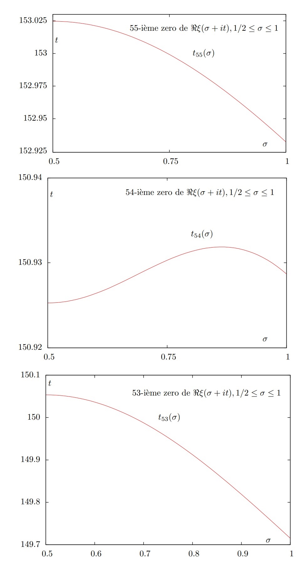
Figure 5: The zero contours of ${\rm Re}(\xi(s))$ in the critical strip, obtained by Gélinas using Pari/GP and Gnuplot system in 2017. Picture permission from Gélinas.

4. Zeros outside the critical line

According to the Theorem 1, the function $\Xi(z)$ satisfies Bombieri’s equivalence condition. By Bombieri’s claim, the Riemann hypothesis holds. This also means that the $\Xi(z)$ function will have no zeros in the whole $z$-plane except for the critical line. Therefore, the work is completed as long as Bombieri’s claim is true. Although we trust that Bombieri has a proof for his theorem, it has not yet been found in the public literature. Therefore, we provide an independent proof for the sufficiency part of it to complete this paper. Of course, Bombieri should be credited if his original proof is later found.

Our next task is to search for the zeros of the $\Xi(z)$ function in the critical strip. The traditional method for this, as described by Pólya [17,20], involves finding a function $A(z)$ such that $|A(z)\Xi(z)-1|=B(z)$ is bounded to be smaller than 1, which would then show that $\Xi(z)$ has no zeros. However, finding such an $A(z)$ has never been easy. Our method was motivated by a numerical study of the zero-counters of the $\Xi(z)$ function (either its real part or imaginary part) in the critical strip. Figure 5 shows some zero-counters of the $u(x,y)$ function, which was produced by Gélinas [20,25] using the Pari/GP and Gnuplot system in 2017. The picture shows that the strip can be divided into several sub-domains by these counters. Since $u(x,y)\neq 0$ in each sub-domain, if we can show that the function $v(x,y)\neq 0$ on the counters, then $\Xi(z)$ is guaranteed to be nonzero in the entire strip.

Likewise, instead of using $u(x,y)$-counters, the strip can be divided by zero counters of the $v(x,y)$ function. By doing so, we discovered that, based on Theorem 1, the Cauchy-Riemann equations can be used perfectly to finish the job, and the Bombieri’s equivalence theorem will also be verified.

Lemma 3. There exists $\varepsilon>0$ that forms two $\varepsilon$-domains attached to the critical line $\omega=\{(x,y):0<|x|<\varepsilon\}$ in which the function $\Xi(z)$ has no zeros.

Proof. We first mention a similar work. In 1914, Bohr and Landau [8] showed that almost all zeros are located inside a small domain $|x|<\varepsilon$. In comparison, this lemma excludes the $\varepsilon$-domain except for the line $x=0$.

From (26), we know that $v(0,y)=0$ on the critical line. If $v_{x}(0,y)\neq 0$, then there exists an $\varepsilon_{1}>0$ such that for any nearby point $(x,y)$ where $0<|x|<\varepsilon_{1}$, we have

$$v(x,y)=v_{x}(0,y)x+\mathcal{O}(x^{2})\neq 0.$$ (68)

Obviously, $\varepsilon_{1}$ depends on the distance $|y-y_{m}|$, where $y_{m}$ is a nearby point at which the function $v_{x}(0,y_{m})=0$. If $|y-y_{m}|>0$, then $\varepsilon_{1}=\varepsilon_{1}(y)>0$.

If $(x,y)$ is near a point $(0,y_{m})$ where $v_{x}(0,y_{m})=0$, then from the Cauchy-Riemann equation,

$$\frac{\partial u}{\partial y}=-\frac{\partial v}{\partial x},$$ (69)

we have $u_{y}(0,y_{m})=-v_{x}(0,y_{m})=0$. According to Theorem 1, the curve $u(0,y)$ reaches a local maximum or minimum at the point $(0,y_{m})$, such that $u(0,y_{m})\neq 0$. Since $u(x,y)$ is continuous, there exists an $\varepsilon_{2}=\varepsilon_{2}(y_{m})>0$ such that when $\sqrt{x^{2}+(y-y_{m})^{2}}<\sqrt{2}\varepsilon_{2}$, we have $u(x,y)\neq 0$.

From (69), the point $(0,y_{m})$ is a stationary point of the function $u(0,y)$ on the critical line $x=0$. According to Theorem 1, the number of $y_{m}$ is countable. Therefore, we can define a function on the critical line as follows:

$$\varepsilon_{3}(y)=\left\{\begin{array}[]{ll}\varepsilon_{2}(y_{m}),&{\rm if\ }|y-y_{m}|<\varepsilon_{2}(y_{m}),\\[8.53581pt] \varepsilon_{1}(y),&{\rm otherwise.}\end{array}\right.$$ (70)

We can then calculate the minimum of the function $\varepsilon_{3}(y)$, which must be positive:

$$\varepsilon:=\min\limits_{-\infty<y<\infty}\varepsilon_{3}(y)>0.$$ (71)

Thus, we can set up two $\varepsilon$-domains attached to the critical line:

$$\omega=\{(x,y):0<|x|<\varepsilon\},$$ (72)

in which the functions $u(x,y)$ and $v(x,y)$ cannot be 0 at the same time, meaning that $\Xi(z)$ has no zeros. $\square$

Lemma 4. The function $\Xi(z)$ has no zero in the region $|x|>0$.

Proof. Due to the symmetry of the function $\Xi(z)$, we only need to consider the half-plane where $x>0$. From Lemma 3, there exists an $\varepsilon$-domain $\omega=\{(x,y):0<x<\varepsilon\}$, which can be divided into several sub-domains $\omega_{k}$ ($k=0,\pm 1,\pm 2,\cdots$) depending on whether $v_{x}(0,y)$ is greater than 0 or less than 0. If $v(x,y)$ is positive in $\omega_{k}$, then it is negative in $\omega_{k+1}$, and the boundary between $\omega_{k}$ and $\omega_{k+1}$ is a zero curve $y=\varphi_{k}(x)$, where $v(x,\varphi_{k}(x))=0$. Specifically, we have

$$\omega_{k}=\{(x,y):0<x<\varepsilon,\ \varphi_{k-1}(x)<y<\varphi_{k}(x),\ (-1)^{k}v(x,y)>0\}.$$ (73)

Since $v(x,y)$ is analytic (continuous and differentiable) in $x>0$, we can extend each sub-domain $\omega_{k}$ to fill the entire half-plane:

$$\Omega_{k}=\{(x,y):x>0,\ \varphi_{k-1}(x)<y<\varphi_{k}(x),\ (-1)^{k}v(x,y)>0\}.$$ (74)

The boundary between $\Omega_{k}$ and $\Omega_{k+1}$ is still denoted by $y=\varphi_{k}(x)$, where $v(x,\varphi_{k}(x))=0$.

.....................................................................................................................................................................................................................................................................................................................................................................................................................................................................................................................................................................................................................................................................................................................................................................................................................................................................................................................................................................................................................................................................................................................................................................................................................................................................................................................................................................................................................................................................................................................................................................................................................................................................................................................................................................................................................................................................................................................................................................................................................................................................................................................................................................................................................................................................................................................................................................................................................................................................................................................................................................................................................................................................................................................................................................................................................................................................................................................................................................................................................................................................................................................................................................................................................................................................................................................................................................................................................................................................................................................................................................................................................................................................................................................................................................................................$0$$-u_{y}=v_{x}<0$$-u_{y}=v_{x}>0$$u_{\max}$$u_{\min}$$y=\varphi_{2k+1}(x)$$y=\varphi_{2k}(x)$$y=\varphi_{2k-1}(x)$$\Omega_{2k+1}:v(x,y)<0$$\Omega_{2k}:v(x,y)>0$${\bf e}_{1}$${\bf e}_{2}$$x$$y$

Figure 6: Sub-domains of $\Omega_{k}$ showing values of function $v(x,y)$.

The boundary curves are zero contours of the $v(x,y)$ function. Although they may have complicated geometries, we can first assume that all curves $y=\varphi_{k}(x)$ neither intersect nor bifurcate in the half-plane $x>0$. A general scenario can be expressed by Figure 6. In the sub-domain $\Omega_{2k}$, $v(x,y)>0$. Therefore, on the left boundary $x=0$, we have $-u_{y}=v_{x}>0$, and $u(0,y)$ reaches a minimum $u_{\rm min}<0$ at the corner of $\Omega_{2k}$ and $\Omega_{2k+1}$, which is the starting point of the curve $y=\varphi_{2k}(x)$. We denote two directional vectors along and perpendicular to the curve by

$${\bf e}_{1}=\big{(}1,\ \varphi_{2k}^{\prime}(x)\big{)},\hskip 14.22636pt{\bf e}_{2}=\big{(}-\varphi_{2k}^{\prime}(x),\ 1\big{)}.$$ (75)

Since $v(x,y)>0$ in the sub-domain $\Omega_{2k}$, and $v(x,y)<0$ in the next sub-domain $\Omega_{2k+1}$, We calculate the directional derivative of functions in the vertical direction of the curve $y=\varphi_{2k}(x)$, and then apply the Cauchy-Riemann equation for transformation, obtaining

$$0>\nabla v\cdot{\bf e}_{2} = \Big{(}\frac{\partial v}{\partial x},\ \frac{\partial v}{\partial y}\Big{)}\cdot\big{(}-\varphi_{2k}^{\prime}(x),\ 1\big{)}=-\varphi_{2k}^{\prime}(x)\frac{\partial v}{\partial x}+\frac{\partial v}{\partial y}$$ (76)

$$= \varphi_{2k}^{\prime}(x)\frac{\partial u}{\partial y}+\frac{\partial u}{\partial x}=\nabla u\cdot{\bf e}_{1}.$$

Thus, along the curve, $u(x,\varphi_{2k}(x))<u_{\rm min}<0$. In the same way, it can be shown that along the next curve, $u(x,\varphi_{2k+1}(x))>u_{\rm max}>0$. In conclusion, for any $z=x+{\rm i}y$ where $x>0$, if $(x,y)$ is in one of $\Omega_{k}$, then $v(x,y)\not=0$. Otherwise, $(x,y)$ must be on a curve $y=\varphi_{k}(x)$ where $u(x,y)\not=0$. Therefore, $\Xi(z)\not=0$.

................................................................................................................................................................................................................................................................................................................................................................................................................................................................................................................................................................................................................................................................................................................................................................................................................................................................................................................................................................................................................................................................................................................................................................................................................................................................................................................................................................................................................................................................................................................................................................................................................................................................................................................................................................................................................................................................................................................................................................................................................................................................................................................................................................................................................................................................................................................................................................................................................................................................................................................................................................................................................................................................................................................................................................................................................................................................................................................................................................................................................................................................................................................................................................................................................................................................................................................................................................................................................$0$$-u_{y}=v_{x}<0$$-u_{y}=v_{x}>0$$u_{\max}$$u_{\min}$$y=\varphi_{2k+1}(x)$$y=\varphi_{2k}(x)$$y=\varphi_{2k-1}(x)$$\Omega_{2k+1}:v(x,y)<0$$\Omega_{2k}:v(x,y)>0$$0$$x$$y$$P$$u>u_{\max}$$u<u_{\min}$

Figure 7: Sub-domains of $\Omega_{k}$ showing two curves intersecting at point $P$.

Suppose that two curves, namely $y=\varphi_{2k}(x)$ and $y=\varphi_{2k+1}(x)$, intersect at a point $P$, as shown in Figure 7. From previous work, we know that along the curve $y=\varphi_{2k}(x)$, $u(x,y)<u_{\rm min}<0$, and along the curve $y=\varphi_{2k+1}(x)$, $u(x,y)>u_{\rm max}>0$. Thus, the intersection point $P$ becomes a singular point of $u(x,y)$. This contradicts the fact that $\Xi(z)$ is analytic. Therefore, any two curves will not intersect.

..................................................................................................................................................................................................................................................................................................................................................................................................................................................................................................................................................................................................................................................................................................................................................................................................................................................................................................................................................................................................................................................................................................................................................................................................................................................................................................................................................................................................................................................................................................................................................................................................................................................................................................................................................................................................................................................................................................................................................................................................................................................................................................................................................................................................................................................................................................................................................................................................................................................................................................................................................................................................................................................................................................................................................................................................................................................................................................................................................................................................................................................................................................................................................................................................................................................................................................................................................................................................................................................................................................................................................................................................................................................................................................................................................................................................................................................................................................................................................$${\bf e}_{2} {\bf e}_{1} 0 -u_{y}=v_{x}<0 -u_{y}=v_{x}>0 u_{\max} u_{\min} u_{\max} y=\varphi_{2k+1}(x) y=\varphi_{2k}(x) y=\varphi_{2k-1}(x) \Omega_{2k+1}:v(x,y)<0 \Omega_{2k}:v(x,y)>0 x y u<u_{\min} u>u_{\max} y=\hat{\varphi}_{2k}(x) v(x,y)>0 v(x,y)<0 P \bullet$$

Figure 8: Sub-domains of $\Omega_{k}$ showing one curve bifurcating.

Finally, suppose that one curve, $y=\varphi_{2k}(x)$, bifurcates at a point $P$ and gives rise to a new curve $y=\hat{\varphi}_{2k}(x)$, and two new sub-domains in which $v(x,y)$ takes different signs, as shown in Figure 8. We already know that on the lower boundary $u(x,\varphi_{2k-1}(x))>u_{\rm max}>0$, and on the upper boundary $u(x,\varphi_{2k}(x))<u_{\rm min}<0$. Thus, in $\Omega_{2k}$, $u(x,y)$ is decreasing in the direction perpendicular to the boundary curve, i.e., $\nabla u\cdot{\bf e}_{2}<0$. According to the Cauchy-Riemann equations, $\nabla v\cdot{\bf e}_{1}=-\nabla u\cdot{\bf e}_{2}>0$, i.e., $v(x,y)$ is increasing in the direction along the boundary curve. Since $v(x,y)>0$ in $\Omega_{2k}$, from the $\Omega_{2k}$ side to approach the new curve $y=\hat{\varphi}_{2k}(x)$, there is

$$v(x,\hat{\varphi}_{2k}(x))>0.$$ (77)

But across the new curve $y=\hat{\varphi}_{2k}(x)$, we immediately have $v(x,y)<0$. This means the function $v(x,y)$ is discontinuous on the curve $y=\hat{\varphi}_{2k}(x)$, which contradicts $\Xi(z)$ being analytic. Thus, $y=\varphi_{2k}(x)$ cannot bifurcate, and we complete the proof. $\square$

Based on the Lemmas 3 and 4, we have proved the following result.

Theorem 2. If the $\Xi(z)$ function satisfies Bombieri’s equivalence condition on the critical line where ${\rm Re}(z)=0$, then it has no zeros outside this critical line.

Thus, the Riemann hypothesis is true.

5. The counterexample from Pólya

After the death of J.L.W.V. Jensen, Pólya was given access to his Nachlass and published a fundamental article [18] in German in a Danish journal, which unfortunately was not well known. There, he gave detailed proofs of all the interesting properties of the Riemann $\xi(s)$ function that were found by Jensen. At the end, Pólya was left with deciding whether Jensen had ever found a proof of the Riemann hypothesis, or if Jensen’s contributions could lead to a successful proof of the hypothesis. To settle this issue, he produced a devastating example of an entire function that had almost all the properties of the Riemann $\xi(s)$ function investigated by Jensen, but had zeros off the critical line. Since then, any proofs of the Riemann hypothesis using the Jensen function would have been considered invalid if they apply equally well to Pólya’s counterexample, where the analogue of the Riemann hypothesis fails.

Compared to (17), Pólya’s counterexample is a linear combination of two equalities,

$$\Xi(z)=e^{\frac{1}{2}z^{2}}\Big{(}\cosh(z)+\alpha\Big{)}=\frac{2}{\sqrt{2\pi e}}\int\limits_{0}^{\infty}e^{-\frac{1}{2}t^{2}}\Big{(}\cosh(t)+\alpha\sqrt{e}\Big{)}\cosh(zt){\rm d}t,$$ (78)

where $\alpha$ is a parameter. When $-1<\alpha<1$, the function $e^{\frac{1}{2}z^{2}}\big{(}\cosh(z)+\alpha\big{)}$ has infinite simple zeros on the $y$-axis, which behaves the same way as the Riemann $\xi(s)$ function. However, when $\alpha=1$, since

$$\cosh({\rm i}y)+1=\cos(y)+1=2\cos^{2}\Big{(}\frac{y}{2}\Big{)},$$ (79)

it has infinite zeros of order 2 on the $y$-axis, i.e., $y_{k}=(2k+1)\pi$, for $k=0,\pm 1,\pm 2,\cdots$. And when $\alpha>1$, the function $\cosh(z)+\alpha$ has no zeros on the $y$-axis any more. Instead, the zeros appear in the region $x\not=0$, as $z_{k}=\ln(\alpha\pm\sqrt{\alpha^{2}-1})+{\rm i}2k\pi$. Thus, it is necessary to verify whether Pólya’s example could invalidate the results presented in this paper.

The major dispute with Jensen’s work came from the integral kernel, i.e., Jensen’s function $G(t)$ in (11), which is a Gaussian-type function with a bell-shaped curve as shown in Figure 1. In Pólya’s example, the integral kernel

$$G(t)=\frac{2}{\sqrt{2\pi e}}e^{-\frac{1}{2}t^{2}}\Big{(}\cosh(t)+\alpha\sqrt{e}\Big{)}$$ (80)

is also a Gaussian-type function, but its $\Xi(z)$ function has zeros outside the critical line $x=0$. This fact indicates that owning an integral kernel of a Gaussian-type function is not a sufficient condition for the $\Xi(z)$ function to be zero-free outside the critical line. Theorem 2 can be also stated as, if $\Xi(z)$ has a zero outside the critical line, then it must have a positive local minimum or negative local maximum on the critical line. This is indeed the case for Pólya’s example. From (78),

$$\Xi({\rm i}y)=U(y)=e^{-\frac{1}{2}y^{2}}\big{(}\cos(y)+\alpha\big{)}$$ (81)

does have an infinite number of positive local minima when $\alpha>1$. Thus, in the case of $\alpha>1$, Pólya’s counterexample does not contradict the theorems of this paper.

The next question is why the zeros of order 2 occur on the critical line in Pólya’s counterexample when $\alpha=1$. This actually comes from a different property of the $G(t)$ function. From (80), we can calculate:

$$G^{\prime}(t) = tG(t)-\frac{2}{\sqrt{2\pi e}}e^{-\frac{1}{2}t^{2}}\sinh(t)$$ (82)

$$= tG(t)-\frac{\sinh(t)}{\cosh(t)+\alpha\sqrt{e}}G(t).$$

This equation shows an apparent gap compared to (38), in which $-G^{\prime}(t)/t$ is even lower than $G(t)$. Thus, Pólya’s $G(t)$ decreases to 0 much slower than Jensen’s. After taking the Fourier cosine transform of the two $G(t)$s in (3. Bombieri’s equivalence condition), we get two different $U(y)$ functions. In Pólya’s case, as shown in (81), $U(y)$ has a bound function of $e^{-\frac{1}{2}y^{2}}$, so $U^{\prime}(y)/U(y)\approx-y$. In Jensen’s case, from Lemma 1, the bound is $U(y)=e^{-(\pi/8)y}$ and then $U^{\prime}(y)/U(y)\approx-\pi/8$. Thus, for large $y$, Pólya’s $U(y)$ may create a very high slope $U^{\prime}(y)$ near a zero, which could break the simple zero condition.

We can show the curve geometry for Pólya’s $U(y)$ directly. Differentiating (81), we get:

$$U^{\prime}(y) = -yU(y)-e^{-\frac{1}{2}y^{2}}\sin(y),$$

$$U^{\prime\prime}(y) = (y^{2}-1)U(y)+e^{-\frac{1}{2}y^{2}}(2y\sin(y)+\alpha).$$ (83)

When $\alpha$ approaches 1, a critical value of $\alpha_{c}$ that makes $U(y)\to 0+$, $U^{\prime}(y)>0$, $U^{\prime\prime}(y)<0$ can be found [20] by solving the following equations:

$$\cos(y)+\alpha = 0,$$

$$-\sin(y) \geq 0,$$

$$2y\sin(y)+\alpha \leq 0.$$ (84)

It turns out that $\alpha_{c}\approx 0.98617$. This indicates that when $\alpha\geq\alpha_{c}$, a curve geometry of increasing and concave-upward, i.e., $U(y)>0$, $U^{\prime}(y)>0$, $U^{\prime\prime}(y)>0$, has already formed around a zero, which will eventually change the zero from order 1 to order 2 when $\alpha\to 1$. Figure 9 (calculated in [20]) shows the curve geometry around this zero, which can be compared to Figure 4.

...........................................................................................................................................................................................................................................................................................................................................................................................................................................................................................................................................................................................................................................................................................................................................................................................................................................................................................................................................................................................................................................................................................................................................................................................................................................................................................................................................................................................................................................                            2.93.03.13.23.33.43.5                                     $$-80 -60 -40 -20 U(y)\times 10^{6} y U^{\prime\prime}(y)>0$$020406080 (Pólya) .......................................................................................................

Figure 9: A section of $U(y)$ curve from the Pólya’s function, with $\alpha=0.99$.

Thus, Pólya’s $G(t)$ function has a special property that results in $U(y)>0$, $U^{\prime}(y)>0$, and $U^{\prime\prime}(y)>0$ near a zero when $\alpha\to\alpha_{c}$. This causes the zero to change from order 1 to order 2. In contrast, Jensen’s $G(t)$ function does not possess this property. Therefore, in the case of $\alpha=1$, Pólya’s counterexample does not contradict Theorem 1.

Acknowledgement. The author would like to thank his colleague XUE Jian at CCB Fintech for his helpful validation of this paper. The author greatly appreciates Dr. Jacques Gélinas from Ottawa, Canada for his invaluable comments and providing many useful references. In particular, his reading notes [23], which contain the two inequalities (24) and (25) and Pólya’s counterexample [20,26], played a decisive role in proving Lemma 2 and Theorem 1, and his calculation on the zero counters [20,25] provided motivation to prove Lemmas 3 and 4. The author also appreciates the support from Travor Liu, a talented high school student at the time of writing this paper, for providing many reference materials on the Riemann hypothesis. Additionally, the author thanks Professor YANG Bicheng from Guangdong University of Education, China for his suggestions to improve the paper, and Dr. Yaoming Shi from Shanghai, China for his comment on the bound of the $\xi(s)$ function on the critical line.

Reference

1. Riemann B.: Ueber die Anzahl der Primzahlen unter einer gegebenen Grösse, Monatsberichte der Berliner Akademie der Wissenshaft zu Berlin aus der Jahre 1859 (1860), 671-680; also, Gesammelte math. Werke und wissensch. Nachlass, 2. Aufl. 1892, 145-155.

2. Apostol T. M.: Introduction to Analytic Number Theory, Springer. 5th printing 1998 Edition, (1976).

3. Newman D. J.: Analytic Number Theory (Graduate Texts in Mathematics, Vol. 177), Springer Verlag, (1997).

4. Bombieri E.: Problems of the Millennium: the Riemann Hypothesis. In the web-site of the Clay Mathematics Institute: http://www.claymath.org, (2000).

5. Sarnak P.: Problems of the Millennium: The Riemann Hypothesis. In the web-site of the Clay Mathematics Institute: http://www.claymath.org, (2004).

6. Hadamard, J.: Sur la distribution des zéros de la fonction zeta(s) et ses conséquences arithmétiques. Bull. Soc. math. France 24, 199-220, 1896.

7. de la Vallée Poussin, C.-J.: Recherches analytiques la théorie des nombres premiers. Ann. Soc. scient. Bruxelles 20, 183-256, 1896.

8. Edwards H.M.: Riemann’s zeta function. Academic Press Inc., (1974) 193-195.

9. Hardy G.H.: Sur les zéros de la fonction $\zeta(s)$ de Riemann. Comptes rendus de l’Académie des Sciences, 158 (1914) 1012-1014.

10. Platt D. and Trudgian T.: The Riemann hypothesis is true up to $3\cdot 10^{12}$.
    http://arxiv.org/abs/2004.09765v1, (2020).

11. Jensen J.L.W.V.: Recherches sur la théorie des équations. Acta Mathematica, 36 (1913) 181-195. Traduction de la conférence du 29 et 30 août (1911).

12. Titchmarsh E.C.: The Zeta-Function of Riemann. Cambridge University Press, Cambridge, (1930) p43.

13. Wintner A.: A note on the Riemann $\xi$-function. Journal of the London Mathematical Society, 10 (1935) 82-83.

14. Haviland E.K.: On the asymptotic behavior of the Riemann xi-function. American Journal of Mathematics, 67, (1945), 411-416.

15. Spira R.: The integral representation of the Riemann xi-function. Journal of Number Theory, 3 (1971) 498-501.

16. Matiyasevich Yu V.: Yet another machine experiment in support of Riemann’s conjecture. Cybernetics, 18, (1982), 705-707. Translated from Kibernetika (Kiev) 6, (1982), 10-22.

17. Pólya G.: Bemerkung über die Integraldarstellung der Riemannschen $\xi$-Funktion, Acta Mathematica, 48 (1926), 305-317.

18. Pólya G.: Ueber die algebraisch-funktionentheoretischen Untersuchungen von J.L.W.V. Jensen, Klg. Danske Vid. Sel. Math.-Fys. Medd. 7, (1927), 3-33.

19. Landau E.: Handbuch der Lehre von der Verteilung der Primzahlen. B. G. Teubner, Leipzig, (1909) p288.

20. Lin X.: Calculation details for the article of a proof to the Riemann hypothesis.xlsx, http://github.com/linxiao19570629/rh, (2023).

21. Whittaker E.T. and Watson G.N.: A Course of Modern Analysis, Cambridge University Press, Cambridge, (1927) p524.

22. Romik D.: The Taylor coefficients of the Jacobi theta constant $\theta_{3}$.
    http://arxiv.org/abs/1807.06130, (2018).

23. Gélinas J.: Gélinas 2021 Reading notes on the Riemann xi function - Jensen function Phi(t). http://www.researchgate.net/publication/362385237, (2021).

24. Titchmarsh E.C.: The theory of the Riemann zeta function. Second Edition. Edited and with a preface by D.R. Heath-Brown. The Clarendon Press: Oxford (1986) p29.

25. Gélinas J.: On zero counters of Riemann xi-function from Pari/GP. and Gnuplot system. http://www.researchgate.net/publication/368756557 (2021). Also Gélinas J.: Learning with GP: Griffin, Ono, Rolen, Zaghier asymptotic formula for xi(s),
    http://pari.math.u-bordeaux.fr/archives/pari-users-1908/msg00022.html (2019).

26. Gélinas J.: Solution on Polya’s counterexample for Riemann hypothesis study by Jensen. http://www.researchgate.net/publication/368756617 (2021).