Small-scale clumping at recombination and the Hubble tension

Abstract

Despite the success of the standard $\Lambda$CDM model of cosmology, recent data improvements have made tensions emerge between low- and high-redshift observables, most importantly in determinations of the Hubble constant $H_{0}$ and the (rescaled) clustering amplitude $S_{8}$. The high-redshift data, from the cosmic microwave background (CMB), crucially relies on recombination physics for its interpretation. Here we study how small-scale baryon inhomogeneities (i.e., clumping) can affect recombination and consider whether they can relieve both the $H_{0}$ and $S_{8}$ tensions. Such small-scale clumping, which may be caused by primordial magnetic fields or baryon isocurvature below kpc scales, enhances the recombination rate even when averaged over larger scales, shifting recombination to earlier times. We introduce a flexible clumping model, parametrized via three spatial zones with free densities and volume fractions, and use it to study the impact of clumping on CMB observables. We find that increasing $H_{0}$ decreases both $\Omega_{m}$ and $S_{8}$, which alleviates the $S_{8}$ tension. On the other hand, the shift in $\Omega_{m}$ is disfavored by the low-$z$ baryon-acoustic-oscillations measurements. We find that the clumping parameters that can change the CMB sound horizon enough to explain the $H_{0}$ tension also alter the damping tail, so they are disfavored by current Planck 2018 data. We test how the CMB damping-tail information rules out changes to recombination by first removing $\ell>1000$ multipoles in Planck data, where we find that clumping could resolve the $H_{0}$ tension. Furthermore, we make predictions for future CMB experiments, as their improved damping-tail precision can better constrain departures from standard recombination. Both the Simons Observatory and CMB-S4 will provide decisive evidence for or against clumping as a resolution to the $H_{0}$ tension.

I Introduction

The standard $\Lambda$-cold dark matter ($\Lambda$CDM) model of cosmology has proven to be remarkably successful in interpreting different measurements consistently and simultaneously. These include the cosmic microwave background (CMB, for example [1, 2]), the large-scale structure (LSS, e.g. [3, 4, 5]), and probes of the expansion rate of the Universe (such as [6, 7]). However, as the precision of these probes has increased, tensions between them have started to appear.

A notable problem that has emerged within $\Lambda$CDM is the Hubble tension—a discrepancy between the cosmic expansion rate today (given by the Hubble parameter $H_{0}$) inferred from different data sets. On the one side, the standard CMB analysis of Planck 2018 data yields a value of $H_{0}=\left(67.4\pm 0.5\right)$ km s^-1 Mpc^-1 [2]. On the other side, direct $H_{0}$ measurements (from type Ia supernovae calibrated with Cepheids [8, 9, 10, 7] or surface brightness fluctuations [11]; from type II supernovae [12], strong-lensing time delays [13, 14, 15], gravitational waves standard sirens [16], Tully-Fisher relations [17], tip of the red giant branch [18], Mira variables [19] or megamasers [20]) give higher values. In this paper, we will focus on the latest distance-ladder measurement of the Supernovae, H0, for the Equation of State of Dark Energy (SH0ES) Collaboration $H_{0}=\left(73.2\pm 1.3\right)$ km/(s Mpc) [7], which is $4.2\sigma$ away from Planck.

There is another, weaker tension in the values of the matter fraction $\Omega_{m}$ and the amplitude of galaxy clustering $\sigma_{8}$ (on spheres of comoving radius $R=8/h$ Mpc). Instead of $\sigma_{8}$, a related parameter $S_{8}=\sigma_{8}\left(\Omega_{m}/0.3\right)^{0.5}$ is often used, as it is less correlated with $\Omega_{m}$ in LSS data. Planck Collaboration et al. [2] report $\Omega_{m}=0.315\pm 0.007$ and $S_{8}=0.831\pm 0.017$ with Planck data, while the Dark Energy Survey Year 1 (DES-Y1, [21]) weak-lensing and galaxy-clustering data obtains $\Omega_{m}=0.264^{+0.032}_{-0.019}$, $S_{8}=0.783^{+0.021}_{-0.025}$. The new DES Year 3 results are $\Omega_{m}=0.339^{+0.032}_{-0.031}$, $S_{8}=0.776\pm 0.017$ [5], making the tension weaker, but still worth exploring, as other LSS probes disagree with the CMB [22, 23, 24, 25, 26, 27].

Various extensions to $\Lambda$CDM have been proposed to solve the $H_{0}$ discrepancy. They can be broadly divided into early- and late-type solutions, with the former changing the length of the standard ruler [28, 29, 30, 31, 32], and the latter the evolution of the expansion rate $H(z)$ at low redshifts [33, 34, 35, 36]. Only the early-type solutions can be in agreement with low-$z$ standard-ruler measurements of the BAOs, though the most popular model of early dark energy [37] worsens the $S_{8}$ tension (for a recent review see Knox and Millea [38]). Here, instead, we study how changing the physics of recombination is an early-type solution to both the $H_{0}$ and $S_{8}$ tensions, as first proposed in [39].

The interpretation of CMB data crucially relies on the physics of recombination, so it is natural to ask how well understood, and constrained, this transition is. The process of hydrogen recombination depends crucially on the two-body recombination rate, and thus can be affected by physics at very small scales [40]. In [41, 42, 43] it was shown that, by creating baryonic clumping at small scales, primordial magnetic fields (PMFs, for a review see Subramanian [44]) would leave an imprint on the CMB by allowing a more-rapid process of recombination, and shifting the decoupling between photons and baryons to larger $z$. While such inhomogeneities would take place at very small scales, they enhance the recombination rate when averaged over larger scales. An earlier recombination implies a higher $H_{0}$ for a fixed angular sound horizon $\theta_{s}$ in the CMB. Recently, Jedamzik and Pogosian [39] have shown that such a clumping could relieve both the Hubble and $S_{8}$ tensions in current cosmological data. On the other hand, Thiele et al. [45] argued that the $H_{0}$ value inferred from Planck and Atacama Cosmology Telescope (ACT) data remains in significant tension with SH0ES.

Here we extend previous analyses by introducing a very generic model of clumping at small scales. This model posits that baryons live in three zones: an average one, and an over/underdense one (see Fig. 1). This encompasses the models in Jedamzik and Pogosian [39] and Thiele et al. [45], as well as other possible origins of small-scale baryonic clumps, such as baryon isocurvature [46].

The key question we tackle is whether a change in recombination that is sufficient to change the sound horizon—and thus explain the $H_{0}$ tension—leaves a detectable imprint on the CMB damping tail. The high-$\ell$ CMB tail has been measured to great success by the Planck, ACT [47], and South Pole Telescope (SPT, [48]) collaborations; and upcoming measurements from the Simons Observatory (SO, [49]) and CMB-S4 [50] will improve those measurements even further.

This paper is structured as follows. We start in Sec. II by defining our generalized clumping model (M3), and discussing its physical implications in Sec. III. In Sec. IV we analyze the current CMB data from Planck 2018 [51, 52], exploring clumping-$H_{0}$ correlations as well as looking into shifts in $S_{8}$ and $\Omega_{m}$. Then we perform forecasts for future CMB experiments in Sec. V, to understand how better measurements of the damping tail will test our clumping model more precisely. We conclude in Sec. VI.

II Three-zone model (M3) for recombination

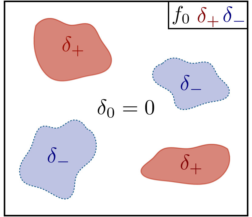
Figure 1: M3 spatial structure: regions with average ($0$), lower ($-$) and higher ($+$) density. We take those three effective zones to have constant overdensity $\delta_{i}=n_{H,i}/\left\langle n_{H}\right\rangle-1$ each, and the structure is fixed in time. The model is described by six parameters: three $\delta_{i}$’s and three volume fractions $f_{i}$ that each zone occupies. There are three constraints: $\sum_{i}f_{i}=1$, $\sum_{i}f_{i}\delta_{i}=0$ and $\delta_{0}=0$. So we choose $f_{0}$ and $\delta_{\pm}$ as input parameters, as highlighted in upper right corner.

We begin by defining our three-zone model (M3) for baryonic clumping. The general idea is that there are fluctuations on very small ($\sim$ kpc for PMFs [44]) scales, so that the large-scale behavior of baryons follows the usual assumptions; whereas the recombination rate, which depends on the electron density squared ($n_{e}^{2}$) can be enhanced (for large overdensities) or reduced (for underdensities), with respect to the average.

Our general picture is illustrated in Fig. 1: there are regions with average (marked by the index $0$), lower ($-$) and higher ($+$) density. For simplicity, we take those three effective zones to have constant hydrogen density $n_{H}$ each, and the structure is constant in time. Then one needs six parameters: three weights (volume fractions) $f_{i}$ and three densities, which can be parametrized as $\Delta_{i}=n_{H,i}/\left\langle n_{H}\right\rangle$ or $\delta_{i}=\Delta_{i}-1$ (hereafter $i=\left\{0,-,+\right\}$). However, we set three constraints: first, all volume is divided between the three zones ($\sum_{i}f_{i}=1$), second, the total baryonic mass is set by $\omega_{b}$ ($\sum_{i}f_{i}\Delta_{i}=1$, or equivalently $\sum_{i}f_{i}\delta_{i}=0$), and finally, one of the zones has average density ($\delta_{0}=0$, which is optional but simplifies the analysis). This leaves three free parameters. For input, we choose the two nonzero relative overdensities $\delta_{-}$, $\delta_{+}$ and the volume fraction $f_{0}$ of the average-density zone.

This three-parameter model is very flexible, as for example it encompasses the M1 and M2 models presented in Jedamzik and Pogosian [39] (obtained by fixing $f_{0}=1/3$, and either $\delta_{-}=-0.9$ for M1 or $\delta_{-}=-0.7$ for M2). However, our M3 model is only bound by the constraints of volume and mass conservation and the only arbitrary choice is setting one of the three regions to have average density. On the flip side, this flexibility makes the three parameters very degenerate: if either $f_{0}\rightarrow 1$, $\delta_{+}$ or $\delta_{-}\rightarrow 0$, then the deviation from uniform density becomes negligible.

Therefore, the prior on these parameters ought to be balanced between generality and degeneracy. We choose a log-uniform prior on $\left|\delta_{-}\right|$ ($10^{-5}\leq\left|\delta_{-}\right|\leq 0.955$) and on the ratio $\left|\delta_{+}/\delta_{-}\right|$ ($0.1\leq\left|\delta_{+}/\delta_{-}\right|\leq 10$), and a uniform prior on $f_{0}$ ($0\leq f_{0}\leq 1$). The lower bound on $|\delta_{-}|$ is set to the curvature perturbations $\sqrt{A_{s}}\sim 10^{-5}$, whereas the higher bound is determined by numerical limitations of the recombination code, more extreme underdensities cause the integration in RECFAST to fail. Bounds on the ratio are chosen so that the under and overdensity regions are within an order of magnitude from each other, to avoid the unnatural configuration when one $\delta$ is negligible and other is significant. Moreover, the constraints force the volume fractions ratio to be $f_{+}/f_{-}=-\delta_{-}/\delta_{+}$, so very different $\delta$’s will cause one of the volume fractions to be tiny and the whole clumping effect negligible.

An important parameter quantifying the amplitude of the inhomogeneities is the relative variance of densities,

$$b=\frac{\left\langle\left(n_{H}-\left\langle n_{H}\right\rangle\right)^{2}\right\rangle}{\left\langle n_{H}\right\rangle^{2}}=-\delta_{-}\delta_{+}\left(1-f_{0}\right),$$ (1)

hereafter denoted as the clumping parameter $b$, following Jedamzik and Pogosian [39].

Technically, we implement this model in a fork of the CLASS code [53]. We run the standard recombination code RECFAST [54, 55, 56] within each zone separately, given its density $n_{H,i}$, producing three recombination histories, in terms of their free electron fractions $x_{e,i}\left(z\right)=n_{e,i}/n_{H,i}$. These are then averaged

$$x_{e}\left(z\right)=\sum_{i}f_{i}\Delta_{i}x_{e,i}\left(z\right)$$ (2)

and passed to the rest of modules in CLASS.

We also have tested our method with the more precise recombination code HyREC [57]. While the two codes differ in their predictions of the highest $\ell$ modes (see e.g. Lee and Ali-Haïmoud [58]), we find this difference subleading for the purposes of this paper, as shown in Appendix A.1.

III The effects of small-scale gas clumping on the CMB

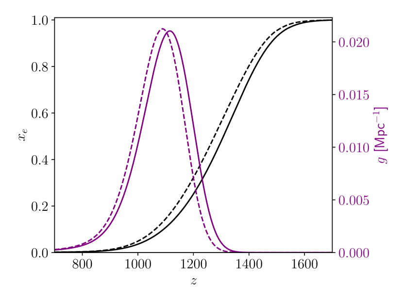
Figure 2: Demonstration of the effect of clumping on the recombination history ($x_{e}$, black) and visibility function ($g$, purple) versus redshift $z$. Standard recombination is shown as dashed curves, and clumping in solid, where we have set $\delta_{-}=-0.9$, $\delta_{+}=5/3$, and $f_{0}=1/3$, to yield $b=1$. Cosmology ($\theta_{s}$, $\omega_{b}$, $\omega_{\mathrm{cdm}}$, $A_{s}$, $n_{s}$, $\tau_{\mathrm{reio}}$) is fixed to the Planck best fit [2].

III.1 Recombination

Consider the recombination of an effective three-level hydrogen atom,

$$\frac{dn_{e}}{dt}+3Hn_{e}=-\left(\alpha n_{e}n_{H^{+}}-\beta n_{H^{0}}e^{-E_{21}/kT}\right)C,$$ (3)

where $\alpha$ and $\beta$ are recombination and photoionization rate coefficients, $E_{21}$ is the energy difference between the first excited level and the ground state, $k$ is Boltzmann constant, $T$ is temperature and $C$ is an additional factor taking into account both Lyman-$\alpha$ and two-quantum decays [59, 60]. If we take a spatial average, all terms except the first on the right-hand side, will depend on $\left\langle n_{H}\right\rangle$, while that one term will depend on $\left\langle n_{H}^{2}\right\rangle$, as it corresponds to recombinations (binding of an electron and an ion). Introducing inhomogeneities enhances the average recombination rate, as $\left\langle n_{H}^{2}\right\rangle\geq\left\langle n_{H}\right\rangle^{2}$ (where equality is only reached for uniform density). This causes $n_{e}$ to decrease faster, and the Universe to become neutral and transparent to radiation earlier than in the homogeneous case. Given a recombination history, we define the visibility function

$$g=\dot{\tau}e^{-\tau}$$

as the probability that a CMB photon last scattered per unit conformal time, and thus determines the effective redshift of recombination. It is given in terms of the Thomson optical depth $\tau$ and its derivative with respect to conformal time $\eta$ (namely the inverse of photon’s comoving mean free path),

$$\dot{\tau}=\sigma_{T}n_{H,\rm now}x_{e}\left(1+z\right)^{2},$$ (4)

where $n_{H,\rm now}$ is hydrogen number density today, which is not time- or redshift-dependent, and $\sigma_{T}$ is Thomson scattering cross-section.

While Eq. (3) is a simple approximation—and in our implementation we include the detailed physics of the recombination codes—it serves to illustrate how small scales affect recombination at large scales. As an example, Fig. 2 shows how clumping affects recombination, where the intuition from Eq. (3) remains true: clumping shifts recombination and thus the peak of the visibility function to higher redshifts.

To show how recombination evolves in over/under-dense regions, we plot the ionization fraction in each of the three zones of our M3 model in Fig. 3. The underdense (‘‘-’’) zone has a dramatically delayed recombination history, and it presents a sizable low-$z$ tail. The total M3 ionization fraction approaches the ‘‘0’’ zone (namely standard recombination) for lower redshifts.

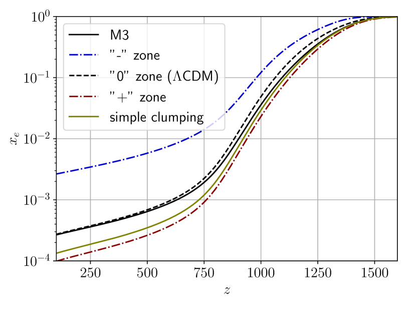
Figure 3: Ionization fraction in different zones of the M3 and simple-clumping models. The clumping parameters are $\delta_{-}=-0.9$, $\delta_{+}=5/3$, and $f_{0}=1/3$, $b=1$. Cosmology ($\theta_{s}$, $\omega_{b}$, $\omega_{\mathrm{cdm}}$, $A_{s}$, $n_{s}$, $\tau_{\mathrm{reio}}$) is fixed to the Planck best fit [2]. The ‘‘-’’ zone behaves very different from the others and has a notable low-redshift tail. The total M3 ionization fraction approaches the ‘‘0’’ zone (namely standard recombination), while for simple clumping (when rates of recombination and other two-body processes are just enhanced by a factor of $1+b$) $x_{e}$ stays lower. The simple-clumping model produces larger deviations in power spectra than M3 for the same $H_{0}$ change and is only shown here for comparison purposes.

We note that manually enhancing the average recombination rate (i.e., without keeping track of the overdense and underdense zones) does not capture the entire effect of clumping. To illustrate that, we have also implemented a simple one-parameter clumping model, using only $b$ [Eq. (1)], where we have assumed a spatially uniform $x_{e}$ and have therefore just multiplied the rates of recombination and other two-body processes by $\left\langle n_{H}^{2}\right\rangle/\left\langle n_{H}\right\rangle^{2}=1+b$ inside RECFAST. From Fig. 3 it is clear that this simple model behaves like an overdense zone and does not reproduce the behavior of M3. Such a difference arises because the recombination rate is proportional to $\left\langle n_{e}n_{H^{+}}\right\rangle\approx\left\langle x_{e}^{2}n_{H}^{2}\right\rangle$. Only if one assumes constant $x_{e}$ can one simply put the latter equal to $\left\langle x_{e}\right\rangle^{2}\left\langle n_{H}^{2}\right\rangle=\left\langle x_{e}\right\rangle^{2}\left\langle n_{H}\right\rangle^{2}\left(1+b\right)$. But if we assume no electron mixing between the zones, at each density the recombination goes at its own pace. At lower densities the ionization fraction is higher and vice versa. Then $\left\langle x_{e}^{2}n_{H}^{2}\right\rangle<\left\langle x_{e}\right\rangle^{2}\left\langle n_{H}\right\rangle^{2}\left(1+b\right)$, and the actual ratio is time-dependent. As a consequence, this simple clumping model causes significantly higher difference in power spectra $C_{\ell}$ for the same change in $H_{0}$ than M3 and thus cannot better alleviate the Hubble tension. This implies that matching the low-$z$ tail of recombination is key for consistency with CMB data. Therefore only M3 and not simple clumping is used further in the paper.

III.2 Sound horizon at last scattering

Shifting the epoch of recombination affects the quantities derived from the CMB. For example, distances are inferred from well-measured CMB angular scales, such as the angular scale of the sound horizon at last scattering $\theta_{s}=r_{s}/r_{*}$, where

$$r_{*}=\int_{0}^{z_{*}}\frac{cdz}{H\left(z\right)}$$ (5)

is the comoving distance to the last scattering surface, $c$ is speed of light, and

$$r_{S}=\int_{z_{*}}^{\infty}\frac{c_{S}\left(z\right)dz}{H\left(z\right)}$$ (6)

is the comoving distance a sound wave (of speed $c_{S}$) could travel before last scattering, called sound horizon. The redshift $z_{*}$ of last scattering is determined by recombination physics (in particular by the peak of the visibility function) and depends on the radiation, baryon, and matter densities,

$$z_{*}=z_{*}\left(\omega_{r},\omega_{b},\omega_{m}\right);\,\omega_{j}=\Omega_{j}h^{2},$$

where $h=H_{0}/[100\,{\rm km/(s/Mpc)}]$.

The angular sound horizon $\theta_{s}\sim 1/\ell_{\rm peak}$ is measured very well from the CMB power spectrum, where $\ell_{\rm peak}$ is the multipole of the first acoustic peak. This leaves two main avenues to obtain a larger $H_{0}$ from the CMB and solve the Hubble tension. Late-type solutions change the $H(z)$ at low redshifts, affecting the distance to last scattering, i.e., $r_{*}$ in Eq. (5). Early-type solutions, on the other hand, change the sound horizon $r_{s}$ in Eq. (6). This can take the form of an increase in $H(z)$, for instance from early dark energy [28, 31, 29]. In our case, however, it is through altering recombination. Clumping changes the $z_{*}\left(\omega_{r},\omega_{b},\omega_{m}\right)$ function, which lowers $r_{s}$ (at fixed $\omega_{i}$); so to keep the same observed $\theta_{s}$, the comoving distance $r_{*}$ must be reduced, yielding higher $H_{0}$.

III.3 Silk damping

Another important phenomenon closely related to recombination physics is Silk diffusion damping [61]. Photons perform a random walk with nonzero mean free path, which smooths their perturbations, making these decay as time passes. A mode with wave number $k$ is suppressed by a factor $\mathcal{D}\left(k\right)$, which can be approximated as

$$\mathcal{D}\left(k\right)=\int_{0}^{\eta_{0}}d\eta\,g(\eta)\exp\left\{-\left[k/k_{D}\left(\eta\right)\right]^{2}\right\},$$ (7)

where the effective diffusion scale is

$$k_{D}^{-2}\left(\eta\right)=\frac{1}{6}\int_{0}^{\eta}d\eta^{\prime}\frac{1}{\dot{\tau}}\frac{R^{2}+16\left(1+R\right)/15}{\left(1+R\right)^{2}},$$ (8)

with $R=3\rho_{b}/4\rho_{\gamma}=\left(3\omega_{b}/4\omega_{\gamma}\right)\left(1+z\right)^{-1}$ [62], where $\rho_{b}$ and $\rho_{\gamma}$ are the physical energy densities of baryons and photons respectively.

As the visibility function is peaked around recombination ($\eta=\eta_{*}$) and normalized ($\int_{0}^{\eta_{0}}d\eta\,g\left(\eta\right)=1$), the damping factor can be approximated by taking out the exponential at peak out of the integral in Eq. (7), yielding $\mathcal{D}\left(k\right)\approx\exp\left\{-\left[k/k_{D}\left(\eta_{*}\right)\right]^{2}\right\}$. This introduces a new length scale into the problem: $r_{D}=2\pi/k_{D}$, which has different parameter dependence from $r_{S}$.

In the simplest case of a constant sound speed, $r_{S}$ scales as $c_{S}\eta_{*}=c_{S}\int_{z_{*}}^{\infty}dz/H(z)$, which is the distance a sound wave can travel up to recombination, whereas $r_{D}$ scales roughly as $\left[\int_{0}^{\eta_{*}}d\eta/(1+z)^{2}\right]^{1/2}=\left[\int_{z_{*}}^{\infty}dzH^{-1}(z)(1+z)^{-2}\right]^{1/2}$, as the comoving mean free path $\dot{\tau}^{-1}$ scales intrinsically as $(1+z)^{-2}$ [Eq. (4)]. As a consequence, the two scales will react differently to changes in the recombination history. In particular, the damping scale receives a larger contribution from lower redshifts, near $z_{*}$, so it is more sensitive to the recombination profile.

Small-scale clumping shifts recombination to earlier times, and with it the peak of $g$, as we showed in Fig. 2 for our M3 model. This will alter the damping scale relative to the sound horizon.

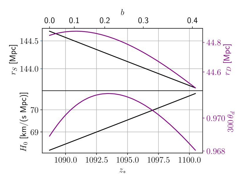
Figure 4: Effects of clumping with a fixed cosmology ($\theta_{s}$, $\omega_{b}$, $\omega_{\mathrm{cdm}}$, $A_{s}$, $n_{s}$, $\tau_{\mathrm{reio}}$), in all cases with $f_{0}=2/3$ and $\left|\delta_{+}/\delta_{-}\right|=4/3$. Top panel: the sound horizon $r_{S}$ (black) decreases with increasing clumping $b$ or recombination redshift $z_{*}$, whereas the damping scale $r_{D}$ (magenta) has a different and more complex behavior. Bottom panel: $H_{0}$ increases (as distance to last scattering $r_{*}$ decreases proportionally to $r_{s}$, and other cosmological parameters are fixed); the angular damping scale $\theta_{d}=r_{D}/r_{*}$ first increases and then decreases.

To build intuition, we have run a sequence of models with increasing clumping but fixed cosmology (in terms of $\theta_{s}$, which is exquisitely measured by the CMB), keeping $f_{0}=2/3$ and $\left|\delta_{+}/\delta_{-}\right|=4/3$ in our M3 model. The effects are shown in Fig. 4. The comoving damping scale changes differently from the sound horizon, as we reasoned before. Similarly to $\theta_{s}=r_{S}/r_{*}$, we convert it to an angular scale $\theta_{d}=r_{D}/r_{*}$, which first increases with clumping and then decreases.

CMB fluctuations with higher multipoles $\ell$ are further Silk suppressed, and thus provide a better measurement of the damping scale $k_{D}$. Therefore, good precision in the CMB damping tail provides a strong test of clumping.

We illustrate this in Fig. 5, where we show the relative difference between CMB power spectra, both temperature ($TT$) and polarization ($EE$) from M3 and from $\Lambda$CDM (with standard recombination), given the same cosmological parameters. In particular, the same sound horizon angular scale $\theta_{s}$ ensures that the acoustic oscillations are in phase with one another, otherwise there would be a large oscillating difference between the power spectra. The gradual deviation on smaller scales ($\ell\gtrsim 1500$ in temperature and $\ell\gtrsim 2000$ in polarization) is caused by the damping scale difference. There are also smaller wiggles in the relative difference, which are caused by the change in duration of last scattering [63]. However, they are less significant than the smoother trend.

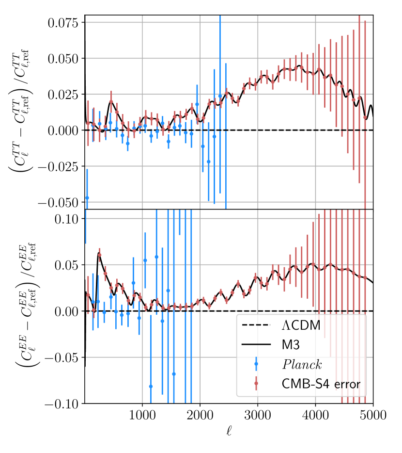
Figure 5: Demonstration of the effect of clumping on the CMB damping tail. We define the $\Lambda$CDM prediction with standard recombination as the reference $C_{\ell,\rm ref}$, and compare our clumping model against it. The black dashed line shows a clumping case, with M3 parameters $\delta_{-}=-0.9$, $\delta_{+}=5/3$, and $f_{0}=1/3$ (giving $b=1$). The cosmological parameters ($\theta_{s}$, $\omega_{b}$, $\omega_{\mathrm{cdm}}$, $A_{s}$, $n_{s}$, $\tau_{\mathrm{reio}}$) are fixed to the Planck best fit. Cyan points represent the binned Planck data, whereas red correspond to CMB-S4 forecasted error bars, both binned with $\Delta\ell=100$.

We also show the Planck measurements and forecasted CMB-S4 binned errors (including both instrumental noise and cosmic variance). Current measurements, from Planck, are scattered around zero, so that it is not easy to tell by eye how strongly this particular clumping configuration is disfavored. However, upon evaluating the likelihood we find $\Delta\chi^{2}_{Planck}=93$, most of it coming from high-$\ell$ ($\ell\geq 30$) $TT,TE,EE$ ($\Delta\chi^{2}_{{\rm high}\,\ell\,TTTEEE}=91$). The difference is high because in this example we have fixed the rest of cosmological parameters. As we will show later (Sec. IV.3, Fig. 9), by shifting the cosmological parameters, M3 is able to fit the $\ell\lesssim 1000$ region very well, though at higher $\ell$ it diverges due to a difference in the damping scale. With CMB-S4 errors, however, the difference induced by $b\sim 1$ clumping is clearly many sigmas in several dozens of bins both in temperature ($TT$) and polarization ($EE$), showing that more precise damping tail measurements will be able to distinguish the presence of significant clumping. For this same example we find $\Delta\chi^{2}_{\rm CMB-S4}\approx 1350$, much higher than for Planck.

IV Results with Planck 2018

In this section we apply the M3 model to Planck 2018 data with the key goal of assessing how it alleviates the Hubble tension. We also perform model comparison ($\Lambda$CDM with standard recombination versus M3) and discuss the compatibility with LSS measurements.

Our CMB datasets are low-$\ell$ $TT,EE$, binned nuisance-marginalized high-$\ell$ $TT,TE,EE$ [51] and lensing [52] power spectra. We also consider the Hubble constant measurement from the SH0ES Collaboration: $H_{0}=\left(73.2\pm 1.3\right)$ km s^-1 Mpc^-1 [7].

We use the Cobaya framework [64] with the Polychord nested sampler [65, 66] for evidences (needed to compute the Bayes factors) and posteriors, and the Py-BOBYQA minimizer [67, 68, 69] for best-fit determinations. Plots are made with anesthetic [70] and GetDist [71].

	Prior	Range
$-\delta_{-}$	Log-uniform	$[10^{-5},0.955]$
$\left|\delta_{+}/\delta_{-}\right|$	Log-uniform	$[0.1,10]$
$f_{0}$	Uniform	$[0,1]$
$\ln(10^{10}A_{s})$	Uniform	$[2.55,3.55]$
$n_{s}$	Uniform	$[0.9,1.05]$
$100\theta_{s}$	Uniform	$[0.95,1.15]$
$\Omega_{b}h^{2}$	Uniform	$[0.02,0.025]$
$\Omega_{\mathrm{cdm}}h^{2}$	Uniform	$[0.1,0.15]$
$\tau_{\mathrm{reio}}$	Uniform	$[0.01,0.2]$
$\Omega_{K}$	Fixed	0
$m_{\nu}$ [eV]	Fixed	0
$A_{planck}$ ($y_{cal}$)	Normal	$1\pm 0.0025$

Table 1: Parameters used in this work and their priors. $\delta_{\pm}$ and $f_{0}$ are only for M3 model, $A_{planck}$ ($y_{cal}$)—for Planck likelihoods.

Our parameters and priors are described in Table 1. It is important to state that we assumed massless neutrinos throughout the sampling to save computing time, as massive neutrinos slow the Boltzmann solver by a factor of $\sim 10$. This assumption shifts upwards the inferred $H_{0}$ values, but it does not affect the changes introduced by M3 (relative to $\Lambda$CDM with standard recombination) in a meaningful way, as we demonstrate in Appendix A.2.

Full contour plots for the M3 clumping model are presented in Appendix B; here we will focus on particular important subspaces.

IV.1 $H_{0}$ and model comparison

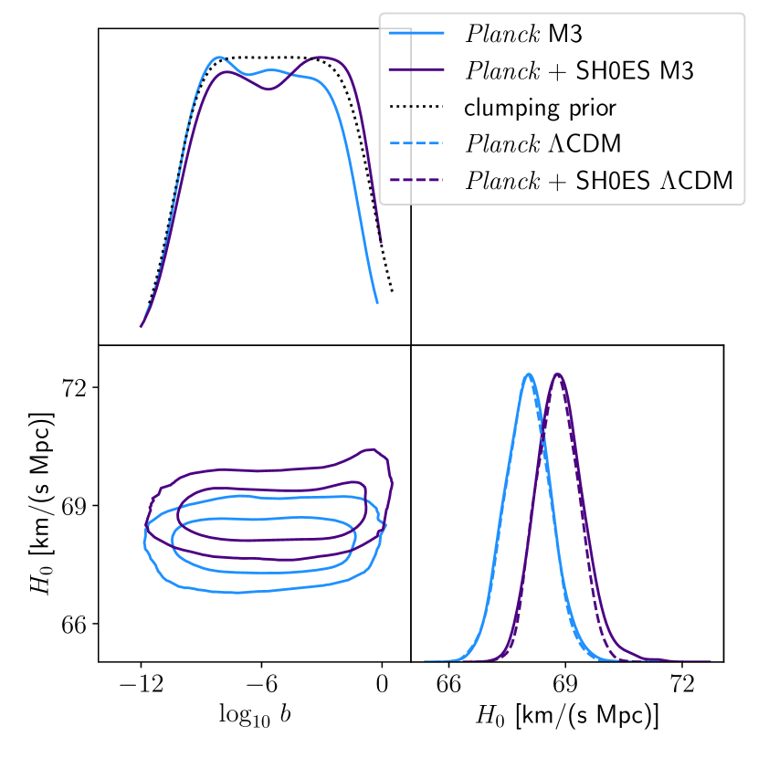
Figure 6: Posteriors for $H_{0}$ and the clumping parameter $b$ of our M3 model [see Eq. (1) for its definition]. We show 68% and 95% CL ellipses using Planck 2018 data alone and in combination with SH0ES, which slightly increases $H_{0}$ though does not prefer clumping. We also show the $H_{0}$ posteriors from $\Lambda$CDM runs with standard recombination, as well as the prior on $b$ for comparison. The 68% C.L. intervals on clumping within M3 are $\log_{10}\,b=-5.9\pm 2.7$ for Planck, $\log_{10}\,b=-5.3^{+4.2}_{-3.7}$ for Planck+SH0ES (and $\log_{10}\,b=-5.5\pm 3.0$ for prior). Neither Planck only nor Planck+SH0ES data prefer large clumping ($b\sim 1$).

We show the 2D posterior for the clumping parameter $b$ and $H_{0}$ in Fig. 6. Planck-only data show no noticeable change in $H_{0}$ compared to $\Lambda$CDM with standard recombination, and some preference against high clumping compared to the prior. Adding a direct $H_{0}$ measurement, however, creates a weak preference for high clumping and high $H_{0}$. Because most of the posterior weight for the clumping parameter $b$ is below unity, we observe almost no correlation between $b$ and $H_{0}$.

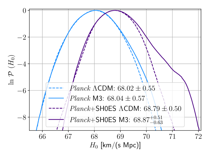
Figure 7: Posterior of $H_{0}$ inferred from Planck data, without and with SH0ES, which shifts the $H_{0}$ values upward as expected. The legend shows 68% C.L. intervals.

In order to explore the tail of the $H_{0}$ posterior distribution, we show it in Fig. 7. With Planck-only data, M3 allows for a weak bump towards higher $H_{0}$ (compared to standard recombination), whereas the mean is not significantly shifted. For Planck data combined with SH0ES, the bump at higher $H_{0}$ for M3 is stronger, given the additional pull from direct $H_{0}$ measurement, though the shift in the mean is still not significant [$\Delta H_{0}=0.08$ km/(s Mpc)].

	$\Delta\chi^{2}_{best}$	$\log_{10}K$
Planck	0	$0.04\pm 0.15$
Planck+SH0ES	5	$0.14\pm 0.19$

Table 2: Model comparison between M3 and $\Lambda$CDM by best-fit $\chi^{2}$ difference and Bayes factor $K$ between M3 and $\Lambda$CDM with Planck 2018 data. $\chi^{2}$ differences rounded to integers because of uncertainty in the minimizer output. M3 does not fit Planck data alone better than $\Lambda$CDM. With SH0ES, M3 allows for slightly better agreement. Bayes factors $-0.5\lesssim\log_{10}K\lesssim 0.5$ show no clear preference between models [72].

We show the best-fit $\chi^{2}$ differences and Bayes factors $K$ between M3 and $\Lambda$CDM models in Table 2. We have not found a better M3 fit to Planck 2018 data alone, compared to $\Lambda$CDM with standard recombination. M3 is more successful than $\Lambda$CDM when considering Planck+SH0ES, but $\Delta\chi^{2}\approx 5$ can not justify three extra parameters. The Bayes factor $K$ in both cases is consistent with 1 (within $<1\sigma$), meaning no preference to either model. The Bayes factor is equal to the ratio of marginalized posterior probabilities of the models if they are assumed equally probable a priori; more generally, posterior probabilities ratio is given by the Bayes factor times prior probabilities ratio [72]. The best-fit parameters are presented in Appendix C, Table 7.

We conclude that M3 is neither supported by the data nor rejected. This is probably not surprising, since Planck data are fit well by $\Lambda$CDM with standard recombination and with an $\approx 4\sigma$ tension between Planck and SH0ES it is challenging to get a detection in a three-parameter model. One could get more support for M3 by considering additional $H_{0}$ data. Here, however, we will limit ourselves to the SH0ES measurement.

IV.2 Low-$\ell$ Planck data analysis

In order to build intuition, we now check whether it is the damping tail that prevents Planck 2018 data from preferring M3. For that, we perform an analysis with only the $\ell<1000$ multipoles. This range of scales is chosen to determine the sound horizon angular scale, though not the damping tail.

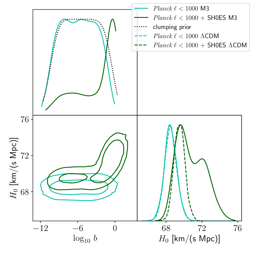
Figure 8: Confidence regions for clumping $b$ versus $H_{0}$ from Planck 2018 $\ell<1000$ data. The absence of damping tail information from the high-$\ell$ data allows significant clumping, and thus larger $H_{0}$. The 68% C.L. intervals on clumping within M3 are $\log_{10}\,b=-5.9\pm 2.8$ for Planck $\ell<1000$, $\log_{10}\,b=-2.8^{+2.9}_{-6.3}$ for Planck $\ell<1000$ + SH0ES (and $\log_{10}\,b=-5.5\pm 3.0$ for prior). Within M3, $H_{0}=(68.51\pm 0.68)$ km/(s Mpc) for Planck $\ell<1000$, $H_{0}=(70.8\pm 1.5)$ km/(s Mpc) for Planck $\ell<1000$ + SH0ES. The $H_{0}$ posteriors from $\Lambda$CDM runs are also shown, which do not reach the high $H_{0}$ values available to M3.

The corresponding 2D posteriors for $b$ and $H_{0}$ are plotted in Fig. 8. Using Planck $\ell<1000$, we find no significant deviation from standard recombination, as the clumping posterior is only slightly shifted from the prior (towards lower values). However, with the additional pull from SH0ES, strong clumping $b\sim 1$ is preferred, and we see a significant bump towards higher $H_{0}$. The best-fit parameters are presented in Appendix C, Table 8.

	$\Delta\chi^{2}_{best}$	$\log_{10}K$
Planck $\ell<1000$	0	$-0.09\pm 0.18$
Planck $\ell<1000$+SH0ES	11	$0.21\pm 0.20$

Table 3: Model comparison with Planck $\ell<1000$ data. $\chi^{2}$ differences are rounded to integers because of uncertainty in the minimizer output. M3 still does not fit the CMB alone better than $\Lambda$CDM, though the joint fit to CMB and SH0ES is improved further than with full Planck. The Bayes factors $K$ show no preference between models, as for full Planck in Table 2.

In order to determine whether clumping provides a better fit in this case, we perform model comparison by two methods: best-fit $\chi^{2}$ and Bayes factor $K$, and show the results in Table 3. We still do not find M3 to fit CMB data notably better than the standard model, with the addition of SH0ES improvement is more significant ($\Delta\chi^{2}_{best}=11$) than in the case of full Planck and SH0ES ($\Delta\chi^{2}_{best}=5$). Bayes factors $K$ are still consistent with one, telling no clear preference between the models. This shows that current Planck data do not prefer clumping as the solution to the $H_{0}$ tension, even without its damping tail.

IV.3 Damping scale

As we have shown in the previous subsection, considering only $\ell<1000$ multipoles from the Planck data opens more room for clumping than using the full data. We posit that the key source of constraints on clumping is the damping-tail information contained in higher-$\ell$ multipoles. So now we consider how the damping tail varies within our M3 model.

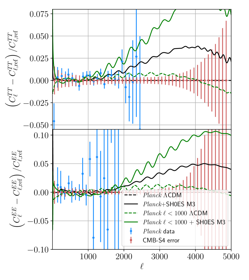
Figure 9: Relative difference in CMB temperature $TT$ and polarization $EE$ power spectra between our best fits (Appendix C, Tables 7, 8), with the $\Lambda$CDM best fit to Planck taken as reference. Differences are small in the low-$\ell$ regime, but grow at smaller scales. Planck data can barely distinguish them, but CMB-S4 will do so very clearly.

First, we plot relative difference in $TT,EE$ power spectra between the best fits in Fig. 9. Unlike in Fig. 5, where the cosmology was kept fixed, producing significant differences, here all the models manage to shift the parameters to fit the low-$\ell$ data. However, they diverge significantly in the damping tail ($\ell\gtrsim 1500$), and CMB-S4 will be able to measure such deviations. More precisely, the $\chi^{2}$ difference between Planck $\Lambda$CDM and Planck+SH0ES M3 best fits from Planck temperature, polarization and lensing is only $\Delta\chi^{2}_{Planck}\approx 4$, while for CMB-S4 precision in temperature and polarization it can be as high as $\Delta\chi^{2}_{\rm CMB-S4}\approx 1030$ (if one assumes the Planck $\Lambda$CDM best fit as fiducial).

In order to build intuition, we formulate the damping-tail constraints in terms of the comoving damping scale $r_{D}$ and its angular analog $\theta_{d}=r_{D}/r_{*}$. We postprocessed the Planck runs to get this information from CLASS.

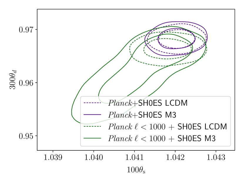
Figure 10: Sound-horizon vs. damping angular scales [both multiplied by a prefactor to make them $\mathcal{O}(1)$] for Planck 2018 + SH0ES runs. The M3 and $\Lambda$CDM contours are quite similar for full Planck+SH0ES (purple). On the contrary, for Planck $\ell<1000$+SH0ES (green), the M3 posterior is significantly extended to lower values of both $\theta_{s}$ and $\theta_{d}$, compared to $\Lambda$CDM.

Figure 10 presents the sound-horizon vs. damping angular scales for our Planck+SH0ES runs. Within $\Lambda$CDM both angular scales are well measured, both for the full Planck data as well as with the $\ell<1000$ modes only. The M3 contours, however, extend to lower values of both $\theta_{d}$ and $\theta_{s}$ compared to $\Lambda$CDM. With full Planck the shift is not significant, while using only $\ell<1000$ allows larger deviations to that region. With Planck $\ell<1000$ + SH0ES, the error bar of $\theta_{d}$ within M3 is by a factor of 3 wider than within $\Lambda$CDM.

We note that the error bar of $\theta_{s}$ is widened similarly. However, the positions of acoustic peaks are not determined exactly by sound horizon angular scale alone. For example, stronger damping would shift the power spectrum maxima to slightly lower $\ell$. Acoustic peak positions may also be affected by fine changes in visibility function shape introduced by clumping. Such small changes might be important, since the characteristic differences in sound horizon scales in our runs are only $\sim 0.1\%$. To assess this, we calculate the positions of first three peaks in $TT$ power spectrum given by CLASS [by fitting Gaussians to $\mathcal{D}_{\ell}=\ell(\ell+1)C_{\ell}/2\pi$, as Planck Collaboration [73]]. We find that M3 keeps peaks at the same positions as $\Lambda$CDM, especially the second one. Therefore we plot second $TT$ peak position instead of $\theta_{s}$ in Fig. 11.

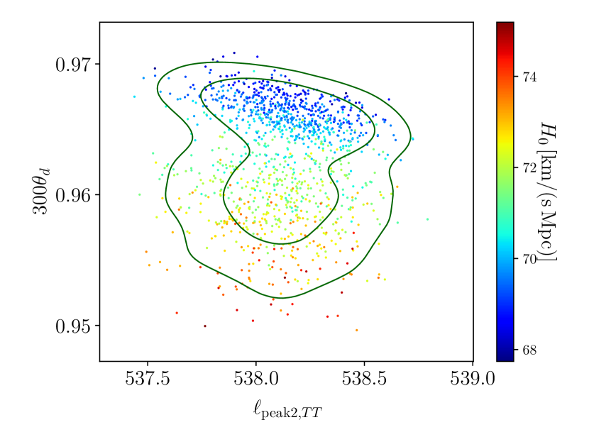
Figure 11: Similar to Fig. 10, but we replace $\theta_{s}$ by position of the second peak in $TT$ power spectrum $\ell_{{\rm peak2},TT}$ and color different points by their value of $H_{0}$, for our Planck $\ell<1000$ + SH0ES M3 run. Within the M3 peak positions stay almost same regardless of $\theta_{d}$. This proves that $\ell<1000$ multipoles from Planck give strong enough constraints on acoustic peaks. In this plane, $H_{0}$ increases for lower values of both $\theta_{d}$ and $\ell_{\rm peak}$. However, the peak positions are measured with $\sim 0.1\%$ precision and do not allow to vary $H_{0}$ significantly with other parameters fixed. This implies that a change in the angular damping scale is necessary to infer higher $H_{0}$ from the CMB.

Figure 11 also shows how $H_{0}$ changes in the $\ell_{{\rm peak2},TT}$-$\theta_{d}$ plane, using Planck 2018 $\ell<1000$ and SH0ES data. The main trend is that $H_{0}$ increases for smaller values of $\theta_{d}$. Therefore, lowering the angular damping scale $\theta_{d}$ is necessary to infer higher $H_{0}$ from CMB. But such change is disfavored by Planck damping tail data. This agrees with our previous subsections, where full Planck + SH0ES did not show a preference for high clumping, and consequently did not exhibit significant change in $H_{0}$, while without $\ell\geq 1000$ multipoles the data allowed for both.

IV.4 $S_{8}$ tension

We now move to discuss whether clumping is compatible with large-scale structure data, which have not been considered in previous subsections.

A potentially interesting discrepancy between the CMB and LSS is the $S_{8}$ tension in the amplitude of matter fluctuations measured from the CMB and the LSS. Planck 2018 reported $\Omega_{m}=0.315\pm 0.007$ and $S_{8}=0.831\pm 0.017$ [2], both of which are higher than found in DES-Y1: $\Omega_{m}=0.264^{+0.032}_{-0.019}$, $S_{8}=0.783^{+0.021}_{-0.025}$ [21]. Earlier recombination (for instance due to small-scale baryon clumping) decreases both the $\Omega_{m}$ and $S_{8}$ values inferred from the CMB, and can therefore help to relieve the $S_{8}$ tension [39].

However, the new DES-Y3 results ($\Omega_{m}=0.339^{+0.032}_{-0.031}$, $S_{8}=0.776\pm 0.017$ [5]) do not show a preference for lower values of $\Omega_{m}$, which makes clumping less favorable resolution. A reanalysis of DES-Y1 data according to the DES-Y3 pipeline shifted the parameter estimates to $\Omega_{m}=0.303^{+0.034}_{-0.041}$, $S_{8}=0.747^{+0.027}_{-0.025}$ [5], in better agreement with Planck on $\Omega_{m}$ but worse on $S_{8}$. Other experiments also find a lower value of $S_{8}$ than Planck and only a small difference in $\Omega_{m}$ ($<1\sigma$), including the Kilo-Degree Survey (KiDS-1000, which reported $\Omega_{m}=0.305^{+0.010}_{-0.015}$, $S_{8}=0.766^{+0.020}_{-0.014}$ [22]), unWISE galaxies (with Planck CMB lensing added, which obtained $\Omega_{m}=0.295\pm 0.017$, $S_{8}=0.776\pm 0.017$ [23]), as well as an analysis of the growth of density perturbations from large-scale structure data (which yielded $\Omega_{m}=0.311^{+0.021}_{-0.028}$, $S_{8}=0.7769\pm 0.0095$ [24], see also [74, 75]).

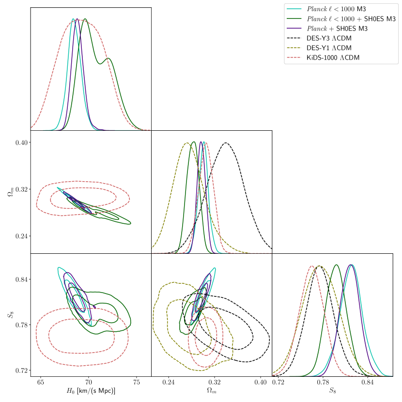
Figure 12: Confidence regions and one-dimensional posteriors for $H_{0}$, matter fraction $\Omega_{m}$ and rescaled clustering amplitude $S_{8}$. Planck $\ell<1000$ M3 has low clumping, therefore is close to $\Lambda$CDM and exhibits similar negative $H_{0}$–$\Omega_{m}$ and $H_{0}$–$S_{8}$ correlations, so increasing $H_{0}$ decreases both $\Omega_{m}$ and $S_{8}$. Planck $\ell<1000$ + SH0ES M3 can reach high clumping (see Fig. 8), giving rise to even lower $\Omega_{m}$ and $S_{8}$. High clumping is disfavored by the damping-tail data of full Planck+SH0ES, so the corresponding contours are closer to $\Lambda$CDM. We show the confidence regions and posteriors from DES-Y3 [5], DES-Y1 [21] and KiDS-1000 [22] for reference. DES data do not constrain $H_{0}$ significantly compared to their prior, which is flat in the range 55 to 91 km/(s Mpc).

To study in detail how clumping interfaces with the $S_{8}$ tension, we show the one-dimensional posteriors and two-dimensional confidence ellipses for $H_{0}$, $\Omega_{m}$ and $S_{8}$ for a few selected runs in Fig. 12. We also show analogous posteriors and contours on $\Omega_{m}$ and $S_{8}$ from DES-Y3 [5], DES-Y1 [21] and KiDS-1000 [22] for comparison. This figure shows that Planck $\ell<1000$ M3 prefers low clumping and therefore is closer to $\Lambda$CDM with standard recombination, exhibiting similar correlations between these three parameters. Note that within $\Lambda$CDM there is a significant negative correlation between $H_{0}$ and $\Omega_{m}$ and a weaker negative correlation between $H_{0}$ and $S_{8}$. Therefore increasing $H_{0}$ alone (for instance by coadding direct $H_{0}$ measurements) decreases both $\Omega_{m}$ and $S_{8}$.

The Planck $\ell<1000$ + SH0ES M3 confidence region exhibits high clumping and explores a different direction, to even lower $\Omega_{m}$ and $S_{8}$. Finally, in full Planck with SH0ES the damping-tail data disfavor high clumping, making the contour close to the standard $\Lambda$CDM.

We note that a rigorous study of the $S_{8}$ tension within M3 would require a reanalysis of the LSS data, as clumping can introduce biases with respect to $\Lambda$CDM with standard recombination. Such an analysis is beyond the scope of this work, and given that this tension is weaker than the $H_{0}$ one, we tentatively conclude that adding LSS data to our runs would not significantly change whether M3 is preferred.

IV.5 Baryon drag scale

As advanced above, the addition of clumping changes the length of the sound horizon due to the nonstandard recombination. This is important for the interpretation of baryon acoustic oscillations (BAO) in galaxy surveys at low $z$, so we now consider how the BAO standard ruler is affected by clumping. The relevant distance is the drag scale $r_{\rm drag}$—the sound horizon at the drag epoch (when the baryon optical depth is 1). The drag epoch occurs slightly later than last scattering, which makes the drag scale larger than the sound horizon $r_{S}$ at last scattering, albeit only marginally.

Standard-ruler BAO measurements constrain the combinations $d_{M}\left(z\right)/r_{\rm drag}$ and $H\left(z\right)r_{\rm drag}$ [4], where $d_{M}$ is the comoving angular-diameter distance. In a flat $\Lambda$CDM cosmology,

$$d_{M}=\int_{0}^{z}\frac{cdz}{H\left(z\right)},$$ (9)

and the dominant contributors are the cosmological constant and the nonrelativistic matter, since for low $z$

$$H\left(z\right)\approx H_{0}\left(1+\Omega_{m}\left[\left(1+z\right)^{3}-1\right]\right)^{1/2}.$$

For a constant $\Omega_{m}$, both $d_{M}\left(z\right)/r_{\rm drag}$ and $H\left(z\right)r_{\rm drag}$ depend only on $H_{0}r_{\rm drag}$. On the CMB side, the sound-horizon angular scale $\theta_{s}$ is also proportional to $H_{0}r_{\rm drag}$ for fixed $\Omega_{m}$, since $r_{\rm drag}$ is very close to $r_{S}$ [see Eq. (6)]. The early integrated Sachs-Wolfe effect in the CMB determines the physical matter density $\omega_{m}=\Omega_{m}h^{2}$, which indeed stays roughly constant in our sampling. Therefore, as $H_{0}$ increases, $\Omega_{m}$ decreases, which causes changes in $d_{M}\left(z\right)/r_{\rm drag}$ and $H\left(z\right)r_{\rm drag}$ at low redshift, compared to their high-redshift analog $\theta_{s}$ (effectively fixed by the CMB). As a consequence, clumping models that fit the CMB develop a tension with BAO data (see Jedamzik et al. [76] for a broader discussion).

As an example, in Fig. 13 we show the relative difference between these quantities for $\Lambda$CDM (best fit to Planck) and for M3 (best fit to Planck+SH0ES), and overlay the SDSS DR12 measurements [4]. By eye, we can tell that the Planck+SH0ES M3 best fit is mildly disfavored by the transversal [$d_{M}\left(z\right)/r_{\rm drag}$] BAO data, while for the radial [$H\left(z\right)r_{\rm drag}$] BAO the data scatter is too large to tell. Using the full covariance matrix, we find $\Delta\chi^{2}_{\rm BAO}\approx-3.6$, indeed mildly disfavoring M3.

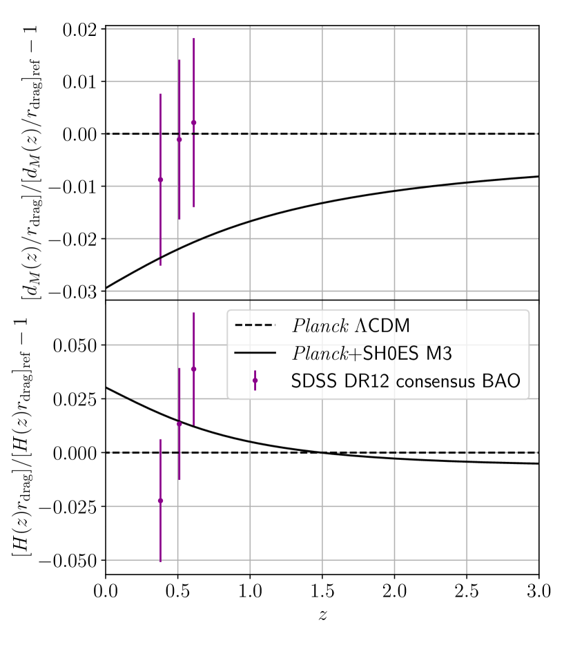
Figure 13: Relative difference in the BAO distances—$d_{M}\left(z\right)/r_{\rm drag}$ and $H\left(z\right)r_{\rm drag}$, for M3 best fit to Planck+SH0ES, compared to the $\Lambda$CDM best fit to Planck (see Appendix C, Table 7 for exact parameters) SDSS DR12 measurements [4] are overlaid. At higher redshifts, the relative difference in $d_{M}/r_{\rm drag}$ tends to 0 and in $Hr_{\rm drag}$—to a negative constant $\approx-0.01$.

At higher redshifts, the relative difference in $d_{M}\left(z\right)/r_{\rm drag}$ tends to 0—so as to match $\approx 1/\theta_{s}$ to the CMB at recombination. The $H\left(z\right)r_{\rm drag}$ relative difference, on the other hand, tends to a negative constant—since $\omega_{m}$ changes weakly, expansion rate at high redshifts is almost the same, so the difference is driven by the change in sound horizon (and thus drag scale), which is $\approx 1\%$ for the Planck+SH0ES M3 best fit compared to Planck $\Lambda$CDM best fit.

While the M3 best fit to Planck+SH0ES is in mild tension with the current BAO measurements, that does not necessarily prove that increasing $H_{0}$ in M3 is always disfavored by BAO data. There remains a possibility that model parameters can be adjusted to accommodate the datasets and provide a better joint fit. To assess this, we plot $d_{M}(z=0.51)/r_{s}$ versus $H_{0}$ for our Planck $\ell<1000$ + SH0ES M3 run in Fig. 14, overlaying the SDSS DR12 measurement. The upper left dots have low clumping, so they follow the standard $\Lambda$CDM degeneracy direction. The right dots, with high clumping, follow a different trend, but still develop more and more tension with SDSS for increasing $H_{0}$, as explained in Jedamzik et al. [76]. We remind the reader that this figure shows only one of three SDSS D12 measurements, and the trend is similar in all, which makes the tension stronger.

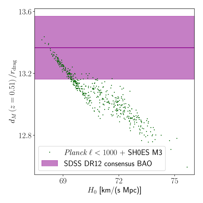
Figure 14: Scatter plot of $d_{M}(z=0.51)/r_{s}$ versus $H_{0}$ for our Planck $\ell<1000$ + SH0ES M3 run, which exhibits the highest clumping. We overplot the SDSS DR12 measurements at this redshift in magenta, where the semitransparent band shows its $1\sigma$ error bar. Even though high clumping (in the right) produces higher $H_{0}$ than inferred from the $\Lambda$CDM degeneracy line (in the upper left), larger values of $H_{0}$ still cause tension between CMB and the BAO.

Standard-ruler BAO data are being improved, and in the future it will become more decisive for or against the clumping model. A notable example is the Dark Energy Spectroscopic Instrument (DESI), which is already operational. DESI is expected to provide subpercent precision measurements of $d_{M}/r_{\rm drag}$ in seven bins for $0.65\leq z\leq 1.25$ [77], which alone can give $\Delta\chi^{2}\approx 20$ between our best-fit models. At higher redshifts, 21-cm data will provide a measurement of $H\,r_{\rm drag}$ to percent-level precision using on velocity-induced acoustic oscillations (VAOs) [78]. Our clumping model predicts only a modest deviation of the radial $H\,r_{\rm drag}$, so transverse BAO measurements have more constraining power.

We note that the change in recombination induced by small-scale clumping is likely to affect the shape of BAO fitting templates, and henceforth the distance-scale extraction from observational data. A proper analysis of BAO data within our M3 model should check whether $d_{M}\left(z\right)/r_{\rm drag}$ and $H\left(z\right)r_{\rm drag}$ are recovered without any biases compared to standard extraction procedures. A quick test with $z=0$ correlation functions in Fig. 15 shows that change in $hr_{\rm drag}$ overwhelms the possible bias in drag scale reconstruction. We leave a detailed study of the correlation function in the presence of clumping for future work.

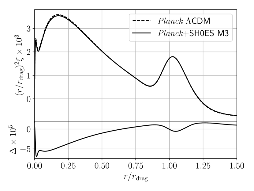
Figure 15: Correlation functions at $z=0$ for $\Lambda$CDM (best fit to Planck) and for M3 (best fit to Planck+SH0ES), rescaled with each baryon drag scale, which gives almost perfect agreement. The lower panel shows the difference between the two lines magnified by an additional factor of 100. The comoving drag scale $r_{\rm drag}$ decreases by 1% between the two cases, but $h$ increases by 4%, so that the drag scale in Mpc/$h$ units $hr_{\rm drag}$ increases by 3%. Such change is clearly noticeable and overwhelms any possible bias arising from template-shape differences.

V Forecasts for future CMB experiments

Having exploited the current data at our disposal, we now perform forecasts for two future CMB experiments: the Simons Observatory (SO, [49]) and CMB-S4 [79], which will have much better damping-tail precision and therefore will be able to test the clumping model much better.

We have written mock likelihoods for these two experiments within Cobaya adapting the ones in MontePython [80, 81], and created the models for these two experiments using deproj0 noise curves for temperature and E-mode polarization fluctuations. We focus on primary CMB anisotropies, rather than lensing map.

	Standard	Clumping
best fit to	Planck	+SH0ES
$\delta_{-}$	n/a (0)	$-$0.955
$\delta_{+}$	n/a (0)	1.320
$f_{0}$	n/a (1)	0.652
$b$	n/a (0)	0.439
$10^{9}A_{s}$	2.1094	2.1132
$n_{s}$	0.96604	0.96552
$100\theta_{s}$	1.04192	1.04177
$\Omega_{b}h^{2}$	0.022416	0.022714
$\Omega_{\mathrm{cdm}}h^{2}$	0.11945	0.11999
$\tau_{\mathrm{reio}}$	0.0514	0.0542
$H_{0}$ [km/(s Mpc)]	68.146	70.916
$\Omega_{K}$	0
$m_{\nu}$ [eV]	0

Table 4: Fiducial parameters for our forecasts.

Throughout this section we consider two fiducial power spectra, which bracket our current knowledge on clumping during recombination: for the first we assume standard recombination ($\Lambda$CDM) and take CMB + direct $H_{0}$ measurement, whereas for the second we choose a model with nonzero clumping and higher $H_{0}$ and consider only CMB. Full parameter sets are presented in Table 4. For each we perform model comparison between M3 and LCDM, and show posteriors for $H_{0}$ and the clumping parameter $b$. For the $H_{0}$ measurement, we assume SH0ES, though we have checked that an $H_{0}$ precision improvement to 1% will not change our conclusions.

V.1 Fiducial with standard recombination

We begin by considering the case that the CMB power spectra of SO/CMB-S4 continue to agree with the standard $\Lambda$CDM model [and a low $H_{0}\approx 68.1$ km/(s Mpc), where the parameters are taken from our best fit to Planck data with massless neutrinos and presented in Table 4]. The question we address is whether the degeneracy between clumping and $H_{0}$ will still be able to bring future CMB experiments in closer agreement with a direct $H_{0}$ measurement in this case. Since our fiducial is $\Lambda$CDM with standard recombination, M3 can not fit the data any better, so model comparison on CMB-only data will not be informative. Therefore, in this subsection we consider only future CMB data added to SH0ES.

We show the model comparison between M3 and $\Lambda$CDM in Table 5. Unlike with Planck, SO/CMB-S4+SH0ES have negligible $\chi^{2}$ improvement. Bayes factors $K$ stay consistent with 1, indicating no clear preference between the models.

	$\Delta\chi^{2}_{best}$	$\log_{10}K$
Planck+SH0ES	5	$0.14\pm 0.19$
SO baseline+SH0ES	0	$0.15\pm 0.22$
CMB-S4+SH0ES	0	$-0.02\pm 0.22$

Table 5: Model comparison forecast with a standard recombination fiducial (see Sec. V.1). All $\chi^{2}$ differences are rounded to integers because of uncertainty in the minimizer output. If CMB data continues to be consistent with standard recombination and low $H_{0}$, M3 will be not able to allow CMB to agree with a direct $H_{0}$ measurement. Bayes factors $-0.5\lesssim\log_{10}K\lesssim 0.5$ tell no clear preference, as in Tables 2 and 3.

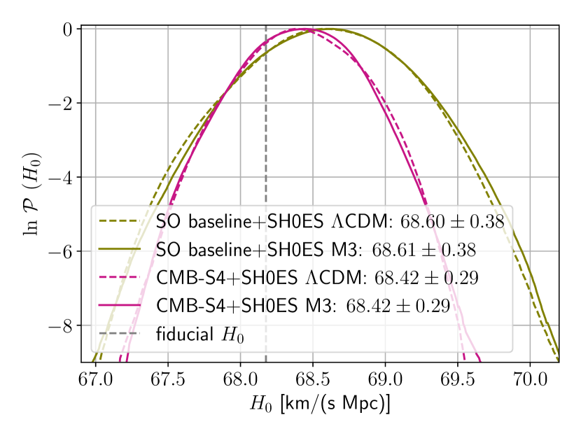
Figure 16: Posterior for $H_{0}$ in our forecasts with a standard recombination fiducial, in all cases with CMB + SH0ES. The solid lines assume M3, whereas dashed assume $\Lambda$CDM with standard recombination. The gray dashed line shows the input fiducial value of $H_{0}$. While the maximum posterior values are shifted to higher $H_{0}$ with respect to the input, due to the addition of a direct $H_{0}$ measurement, the shift from $\Lambda$CDM to M3 is negligible for both experiments. We present 68% C.L. intervals on $H_{0}$ in the legend. For clumping (within M3) they are $\log_{10}\,b=-5.3^{+4.2}_{-3.7}$ for SO+SH0ES, $\log_{10}\,b=-5.8^{+3.7}_{-3.2}$ for CMB-S4+SH0ES (and $\log_{10}\,b=-5.5\pm 3.0$ for prior).

Figure 16 provides a closer look into the $H_{0}$ posterior. If future CMB power spectra continue to agree with $\Lambda$CDM, M3 does not allow any significant $H_{0}$ shift even with the pull from SH0ES. As expected, the increased CMB precision shifts the $H_{0}$ posterior to our input CMB fiducial of $H_{0}\approx 68$ km/(s Mpc), shown as the gray dashed vertical line. The posterior for $b$ is very close to its prior, except that high values $b\sim 1$ are disfavored (and thus does not allow any correlations with $H_{0}$), so we do not show it here.

V.2 Fiducial with clumping

We next investigate a case that in truth contains substantial small-scale clustering. We generate fiducial power spectra for SO/CMB-S4 following the best fit of M3 to Planck+SH0ES, which in particular has $b\approx 0.44$ and $H_{0}\approx 70.9$ km/(s Mpc) (full parameter set in Table 4). In this case our aim is to determine how clearly clumping could be discerned by future CMB data, without any direct $H_{0}$ measurements.

	$\Delta\chi^{2}_{\rm best}$	$\log_{10}K$
Planck	0	$0.04\pm 0.15$
SO baseline	21	${\bf 1.57\pm 0.23}$
CMB-S4	44	${\bf 5.54\pm 0.23}$

Table 6: Same as Table 5, but for a nonzero clumping fiducial (see Sec. V.2). In this case both experiments can show a clear preference for M3, given their large $\Delta\chi^{2}_{\rm best}$. In terms of the Bayes factor $K$, the evidence against $\Lambda$CDM with standard recombination would be strong for SO ($1<\log_{10}K<2$), and decisive for CMB-S4 ($\log_{10}K>2$) [72].

We present the results of our model comparison in Table 6. If there is such clumping in CMB, SO data will show a clear preference for clumping model, and CMB-S4 will be even more decisive. This is the only case when the Bayes factor $K$ is significantly different from 1. With SO data M3 model is deemed $\sim 30$ times more probable than $\Lambda$CDM (strong evidence in favor of M3), and with CMB-S4—$\sim 300,000$ (decisive evidence in favor of M3) [72].

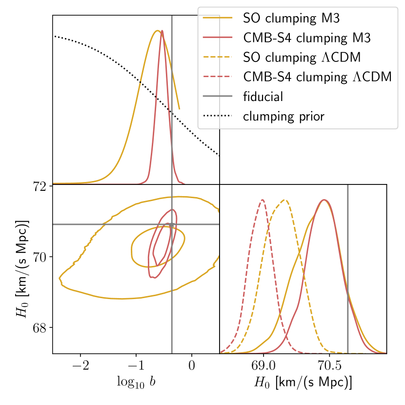
Figure 17: Posteriors of $b$ and $H_{0}$ for forecasts with a clumping fiducial (best fit to current Planck+SH0ES, see Sec. V.2). As is clear from the right panel, M3 and $\Lambda$CDM yield different $H_{0}$ values for the same data (both for SO and CMB-S4). In this case the clumping parameter $b$ will be measured to be nonzero at high significance. The 68% C.L. intervals on clumping within M3 are $\log_{10}\,b=-0.93^{+0.51}_{+0.16}$ for SO, $\log_{10}\,b=-0.53\pm 0.11$ for CMB-S4 (and $\log_{10}\,b=-5.5\pm 3.0$ for prior). Within M3, $H_{0}=70.23^{+0.54}_{-0.47}$ km/(s Mpc) for SO and $H_{0}=(70.36\pm 0.39)$ km/(s Mpc) for CMB-S4.

We show the posteriors of $b$ and $H_{0}$ in Fig. 17, where the difference in $H_{0}$ between standard and clumpy recombination is clear for both SO and CMB-S4. We note that the posteriors for both $H_{0}$ and $b$ peak at lower values than our input fiducials, as lower clumping (and therefore lower $H_{0}$ for the same $\theta_{s}$) is favored by the prior. Also note that all results in this subsection are based on CMB data only, without any direct $H_{0}$ measurements. It is clear that future CMB data alone will suffice to detect clumping, as the posterior becomes much better constrained (against the prior). For SO the lowest values ($b\lesssim 10^{-2}$) are clearly disfavored by the data, whereas for CMB-S4 the limits become only tighter.

VI Conclusions

The Hubble tension poses an increasingly challenging problem to the standard cosmological model. A possible solution is to alter recombination, for instance by adding small-scale baryon clumping, which allows higher $H_{0}$ values to be inferred from CMB data. We have studied whether our flexible clumping model M3, having three spatial zones with variable densities and volume fractions, can solve the tension.

We have found that

1. Current Planck data does not prefer clumping, even when adding the local $H_{0}$ measurement from the SH0ES Collaboration.

2. Including only $\ell<1000$ multipoles, Planck data allow for a larger shift to higher values of $H_{0}$, as the damping tail is more weakly constrained.

3. Increasing $H_{0}$ within $\Lambda$CDM decreases both $\Omega_{m}$ and $S_{8}$. The clumping model M3 follows the same trend, which relieves the potential $S_{8}$ tension with weak-lensing data.

4. However, the same change of $\Omega_{m}$ is in tension with BAO standard-ruler measurements at low $z$. We showed that the BAO template is largely unaltered in the presence of clumping.

We have made forecasts for two future CMB experiments—Simons Observatory and CMB-S4—which will better measure the damping tail. First, we have found that if the power spectra stay consistent with $\Lambda$CDM (i.e., with standard recombination), increasing $H_{0}$ via clumping is strongly disfavored. Second, we have shown that the current best-fit model to Planck+SH0ES with clumping ($b\approx 0.4$) can be detected at high significance based solely on future CMB data. Therefore future CMB experiments will provide considerable diagnostic power to investigate small-scale clumping at the epoch of recombination and shed light onto possible solutions to the $H_{0}$ tension.

VII Acknowledgements

JBM was funded through a Clay fellowship at the Smithsonian Astrophysical Observatory. DJE is partially supported by U.S. Department of Energy Grant No. DE-SC0013718 and as a Simons Foundation Investigator. CD is partially supported by the Department of Energy (DOE) Grant No. DE-SC0020223.

Appendix A JUSTIFYING SIMPLIFICATIONS

A.1 RECFAST vs HyREC

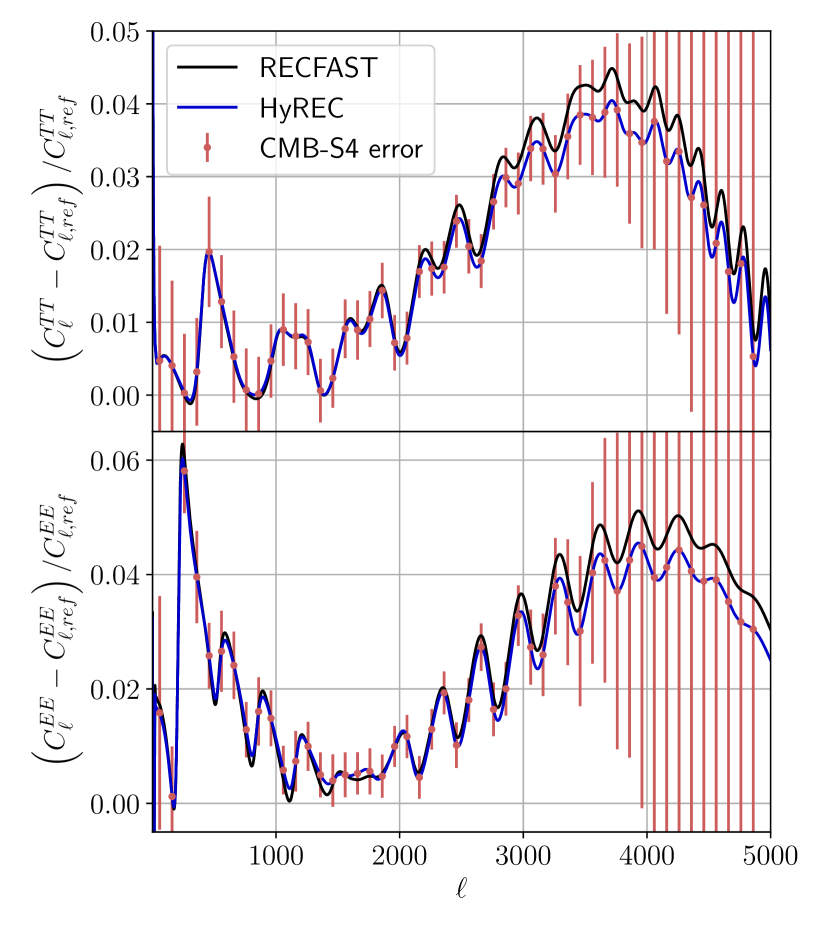
Figure 18: Relative shifts between $\Lambda$CDM with standard recombination (taken as reference $C_{\ell,\rm ref}$) and a particular M3 configuration ($\delta_{-}=-0.9$, $\delta_{+}=5/3$, $f_{0}=1/3$ giving $b=1$, like in Fig. 5), using RECFAST (in black) and HyREC (in blue). The red bands correspond to CMB-S4 errors binned with $\Delta\ell=100$. The cosmological parameters ($\theta_{s}$, $\omega_{b}$, $\omega_{\mathrm{cdm}}$, $A_{s}$, $n_{s}$, $\tau_{\mathrm{reio}}$) are fixed to the Planck best fit.

In the main text we used the recombination code RECFAST, as it is faster than the more precise HyREC; here we justify that this choice does not bias our results. RECFAST is sufficiently accurate for the analysis of Planck data, though this code will not be satisfactory for future CMB missions [58]. Moreover, highly nonstandard hydrogen densities, which can appear in the $\pm$ zones in M3, might limit the RECFAST applicability even further.

For our purposes, the change of zero-point is not the most important, as we focus on the shift introduced by clumping. Therefore, we compare the relative changes in $C_{\ell}^{TT/EE}$ between $\Lambda$CDM with standard recombination and M3 with $b=1$ clumping obtained with RECFAST and HyREC (with full hydrogen model) in Fig. 18. We overlay the CMB-S4 error bars to assess the difference. There is no notable difference for $\ell\leq 2000$-2500, so for current Planck data both codes can be considered equivalent. In particular, the differences between each M3 model and $\Lambda$CDM are $\Delta\chi^{2}_{Planck,\rm RECFAST}=93$ and $\Delta\chi^{2}_{Planck,\rm HyREC}=90$, which are very close (as we note we have not shifted any parameters here). For SO or CMB-S4, however, the difference between the recombination codes can be larger. For the lines shown, $\Delta\chi^{2}_{\rm CMB-S4,RECFAST}=1350$ and $\Delta\chi^{2}_{\rm CMB-S4,HyREC}=1150$, if one assumes the Planck best-fit cosmology (fixed), which shows a relative difference between the recombination codes of $\lesssim 20\%$. Near the fiducial, where most of posterior is, the absolute difference will naturally be lower. Also, for CMB-S4 precision the shifts in parameters are expected to be less than $1\sigma$ [58]. We conclude that an analysis of real SO and CMBS4 data should use HyREC, though RECFAST is sufficient for our forecasting purposes.

A.2 Neutrino masses

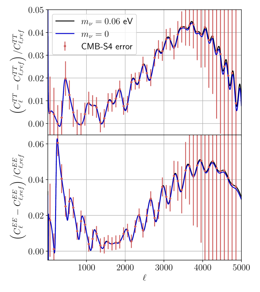
Figure 19: Same as Fig. 18 but comparing the cases of massive (black) and massless (blue) neutrinos.

Throughout this paper we assumed massless neutrinos for efficiency, as it reduces the computational overhead by an order of magnitude. This increases our best fit $H_{0}$ compared to the Planck one. However, again, we are most interested in changes introduced by clumping with respect to standard recombination, so we compare them for massive and massless neutrinos in Fig. 19. The difference between both predictions in this plot is minuscule, and always smaller than even the CMB-S4 error bars. More quantitetively, for the lines shown, $\Delta\chi^{2}_{Planck,m_{\nu}=0.06\,\rm eV}=92.6$ and $\Delta\chi^{2}_{Planck,m_{\nu}=0\,\rm eV}=93.3$; $\Delta\chi^{2}_{{\rm CMB-S4},m_{\nu}=0.06\,\rm eV}=1346$ and $\Delta\chi^{2}_{{\rm CMB-S4},m_{\nu}=0\,\rm eV}=1334$ (if one assumes Planck best fit cosmology for fiducial). The relative difference in $\Delta\chi^{2}$ is $\lesssim 1\%$ in both cases. Therefore computing with massless neutrinos suffices our purposes.

Appendix B FULL CONTOURS FROM PLANCK RUNS

In Fig. 20 we show posteriors for all parameters in runs of M3 with Planck 2018 data (without and with SH0ES). The posteriors on clumping parameters $\log_{10}\left(-\delta_{-}\right)$, $\log_{10}\left|\delta_{+}/\delta_{-}\right|$ and $f_{0}$ are largely flat, like the priors, except the decrease for higher $|\delta_{-}|$ for Planck and increase in the same place for Planck+SH0ES. The clumping parameters also show almost no correlations with standard cosmological parameters, except a weak $H_{0}$ increase for the highest $|\delta_{-}|$. Addition of SH0ES causes some increase in $n_{s}$, $\Omega_{b}h^{2}$, $H_{0}$; a weak increase in $A_{s}$ and $\tau_{\rm reio}$; some decrease in $\Omega_{\rm cdm}h^{2}$.

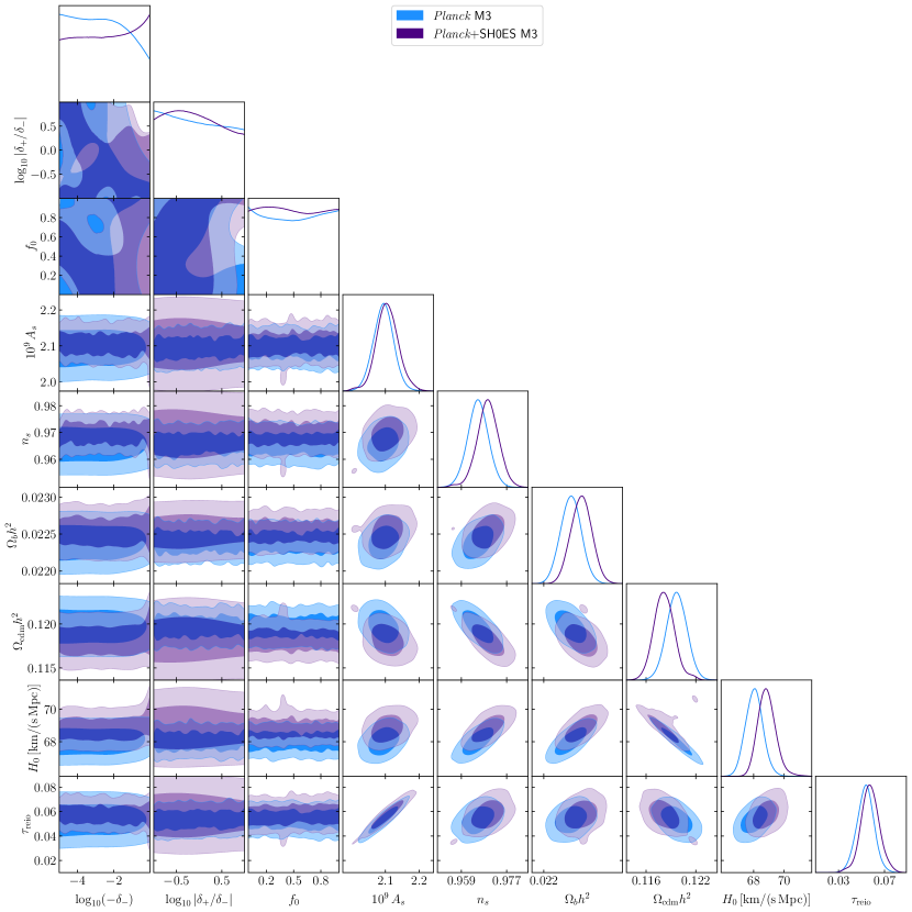
Figure 20: Full contour plot for Planck runs of M3. Purple is with SH0ES, blue is without.

Appendix C BEST FIT PARAMETERS

Model	$\Lambda$CDM	$\Lambda$CDM	M3
Fit to	Planck	Planck+SH0ES
$\delta_{-}$	n/a (0)	n/a (0)	$-$0.955
$\delta_{+}$	n/a (0)	n/a (0)	1.320
$f_{0}$	n/a (1)	n/a (1)	0.652
$b$	n/a (0)	n/a (0)	0.439
$10^{9}A_{s}$	2.1094	2.1440	2.1132
$n_{s}$	0.96604	0.97084	0.96552
$100\theta_{s}$	1.04192	1.04207	1.04177
$\Omega_{b}h^{2}$	0.022416	0.022569	0.022714
$\Omega_{\mathrm{cdm}}h^{2}$	0.11945	0.11762	0.11999
$\tau_{\mathrm{reio}}$	0.0514	0.0555	0.0542
$H_{0}$ [km/(s Mpc)]	68.146	68.993	70.916
$\Omega_{K}$	0
$m_{\nu}$ [eV]	0
$\chi^{2}_{{\rm low}\,\ell\,TT}$	23.2	22.4	23.6
$\chi^{2}_{{\rm low}\,\ell\,EE}$	395.7	396.1	395.9
$\chi^{2}_{{\rm high}\,\ell\,TTTEEE}$	582.2	584.0	585.4
$\chi^{2}_{\rm lensing}$	9.0	8.7	8.8
$\chi^{2}_{\it Planck}$	1010.0	1011.1	1013.7
$\chi^{2}_{\rm SH0ES}$	(15.1)	10.5	3.1

Table 7: Our best fit parameters to (full) Planck and Planck+SH0ES.

In Table 7 we show the best fit parameters when fitting with full Planck data. The M3 best fit to Planck-only is not shown, as we have not found a better one than $\Lambda$CDM, and the $\Lambda$CDM is included in M3 when one sets either one of the $\delta$’s to 0 or $f_{0}=1$. Adding SH0ES in $\Lambda$CDM naturally increases $H_{0}$ as well as most input parameters: $A_{s}$, $n_{s}$, $\theta_{s}$, $\omega_{b}$, $\tau_{\mathrm{reio}}$; whereas $\omega_{\mathrm{cdm}}$ decreases slightly. M3 allows for larger $H_{0}$, while the increase in $A_{s}$ and $\tau_{\mathrm{reio}}$ become smaller, $n_{s}$ and $\theta_{s}$ decrease very slightly, $\Omega_{b}h^{2}$ increases further than in $\Lambda$CDM and $\Omega_{\rm cdm}h^{2}$ increases, unlike in $\Lambda$CDM. The CMB $\chi^{2}$ difference is dominated by high-$\ell$ $TT,TE,EE$ (where ‘‘high’’ means $\ell>30$).

Model	$\Lambda$CDM	$\Lambda$CDM	M3
Fit to	Planck $\ell<1000$	Planck $\ell<1000$ + SH0ES
$\delta_{-}$	n/a (0)	n/a (0)	$-$0.950
$\delta_{+}$	n/a (0)	n/a (0)	1.196
$f_{0}$	n/a (1)	n/a (1)	0.301
$b$	n/a (0)	n/a (0)	0.794
$10^{9}A_{s}$	2.0918	2.1315	2.0705
$n_{s}$	0.97026	0.97711	0.95944
$100\theta_{s}$	1.04150	1.04179	1.04034
$\Omega_{b}h^{2}$	0.022537	0.022773	0.022700
$\Omega_{\mathrm{cdm}}h^{2}$	0.11831	0.11613	0.12198
$\tau_{\mathrm{reio}}$	0.0518	0.0553	0.0505
$H_{0}$ [km/(s Mpc)]	68.528	69.640	72.616
$\Omega_{K}$	0
$m_{\nu}$ [eV]	0
$\chi^{2}_{{\rm low}\,\ell\,TT}$	22.4	21.4	24.8
$\chi^{2}_{{\rm low}\,\ell\,EE}$	395.7	395.9	395.6
$\chi^{2}_{{\rm high}\,\ell\,TTTEEE}$	286.3	288.2	281.5
$\chi^{2}_{\rm lensing}$	8.9	9.0	8.8
$\chi^{2}_{\it Planck}$	713.2	714.4	710.7
$\chi^{2}_{\rm SH0ES}$	(12.9)	7.5	0.2

Table 8: Our best fit parameters to Planck $\ell<1000$, without and with SH0ES.

In Table 8 we show the best fit parameters when fitting with Planck $\ell<1000$ data. The shifts in cosmological parameters are similar and small. Interestingly, the addition of SH0ES helped to find a better fit to Planck than $\Lambda$CDM, unlike with Planck-only data. This is likely because the optimal parameters region with high clumping is small. However, the fit improvement is not significant. The CMB $\chi^{2}$ difference is also dominated by high-$\ell$ $TT,TE,EE$ (where ‘‘high’’ now means $30<\ell<1000$).

References

- Hinshaw et al. [2013] G. Hinshaw, D. Larson, E. Komatsu, D. N. Spergel, C. L. Bennett, J. Dunkley, M. R. Nolta, M. Halpern, R. S. Hill, N. Odegard, L. Page, K. M. Smith, J. L. Weiland, B. Gold, N. Jarosik, A. Kogut, et al., Nine-year Wilkinson Microwave Anisotropy Probe (WMAP) Observations: Cosmological Parameter Results, ApJS 208, 19 (2013), arXiv:1212.5226 [astro-ph.CO] .
- Planck Collaboration et al. [2020a] Planck Collaboration, N. Aghanim, Y. Akrami, M. Ashdown, J. Aumont, C. Baccigalupi, M. Ballardini, A. J. Banday, R. B. Barreiro, N. Bartolo, S. Basak, R. Battye, K. Benabed, J. P. Bernard, M. Bersanelli, P. Bielewicz, et al., Planck 2018 results. VI. Cosmological parameters, A&A 641, A6 (2020a), arXiv:1807.06209 [astro-ph.CO] .
- Eisenstein et al. [2005] D. J. Eisenstein, I. Zehavi, D. W. Hogg, R. Scoccimarro, M. R. Blanton, R. C. Nichol, R. Scranton, H.-J. Seo, M. Tegmark, Z. Zheng, S. F. Anderson, J. Annis, N. Bahcall, J. Brinkmann, S. Burles, F. J. Castander, et al., Detection of the Baryon Acoustic Peak in the Large-Scale Correlation Function of SDSS Luminous Red Galaxies, ApJ 633, 560 (2005), arXiv:astro-ph/0501171 [astro-ph] .
- Alam et al. [2017] S. Alam, M. Ata, S. Bailey, F. Beutler, D. Bizyaev, J. A. Blazek, A. S. Bolton, J. R. Brownstein, A. Burden, C.-H. Chuang, J. Comparat, A. J. Cuesta, K. S. Dawson, D. J. Eisenstein, S. Escoffier, H. Gil-Marín, et al., The clustering of galaxies in the completed SDSS-III Baryon Oscillation Spectroscopic Survey: cosmological analysis of the DR12 galaxy sample, MNRAS 470, 2617 (2017), arXiv:1607.03155 [astro-ph.CO] .
- DES Collaboration et al. [2021] DES Collaboration, T. M. C. Abbott, M. Aguena, A. Alarcon, S. Allam, O. Alves, A. Amon, F. Andrade-Oliveira, J. Annis, S. Avila, D. Bacon, E. Baxter, K. Bechtol, M. R. Becker, G. M. Bernstein, S. Bhargava, et al., Dark Energy Survey Year 3 Results: Cosmological Constraints from Galaxy Clustering and Weak Lensing, arXiv e-prints , arXiv:2105.13549 (2021), arXiv:2105.13549 [astro-ph.CO] .
- Riess et al. [1998] A. G. Riess, A. V. Filippenko, P. Challis, A. Clocchiatti, A. Diercks, P. M. Garnavich, R. L. Gilliland, C. J. Hogan, S. Jha, R. P. Kirshner, B. Leibundgut, M. M. Phillips, D. Reiss, B. P. Schmidt, R. A. Schommer, R. C. Smith, et al., Observational Evidence from Supernovae for an Accelerating Universe and a Cosmological Constant, AJ 116, 1009 (1998), arXiv:astro-ph/9805201 [astro-ph] .
- Riess et al. [2021] A. G. Riess, S. Casertano, W. Yuan, J. B. Bowers, L. Macri, J. C. Zinn, and D. Scolnic, Cosmic Distances Calibrated to 1% Precision with Gaia EDR3 Parallaxes and Hubble Space Telescope Photometry of 75 Milky Way Cepheids Confirm Tension with CDM, ApJ 908, L6 (2021), arXiv:2012.08534 [astro-ph.CO] .
- Freedman et al. [2012] W. L. Freedman, B. F. Madore, V. Scowcroft, C. Burns, A. Monson, S. E. Persson, M. Seibert, and J. Rigby, Carnegie Hubble Program: A Mid-infrared Calibration of the Hubble Constant, ApJ 758, 24 (2012), arXiv:1208.3281 [astro-ph.CO] .
- Burns et al. [2018] C. R. Burns, E. Parent, M. M. Phillips, M. Stritzinger, K. Krisciunas, N. B. Suntzeff, E. Y. Hsiao, C. Contreras, J. Anais, L. Boldt, L. Busta, A. Campillay, S. Castellón, G. Folatelli, W. L. Freedman, C. González, et al., The Carnegie Supernova Project: Absolute Calibration and the Hubble Constant, ApJ 869, 56 (2018), arXiv:1809.06381 [astro-ph.CO] .
- Dhawan et al. [2018] S. Dhawan, S. W. Jha, and B. Leibundgut, Measuring the Hubble constant with Type Ia supernovae as near-infrared standard candles, A&A 609, A72 (2018), arXiv:1707.00715 [astro-ph.CO] .
- Khetan et al. [2021] N. Khetan, L. Izzo, M. Branchesi, R. Wojtak, M. Cantiello, C. Murugeshan, A. Agnello, E. Cappellaro, M. Della Valle, C. Gall, J. Hjorth, S. Benetti, E. Brocato, J. Burke, D. Hiramatsu, D. A. Howell, et al., A new measurement of the Hubble constant using Type Ia supernovae calibrated with surface brightness fluctuations, A&A 647, A72 (2021), arXiv:2008.07754 [astro-ph.CO] .
- de Jaeger et al. [2020] T. de Jaeger, B. E. Stahl, W. Zheng, A. V. Filippenko, A. G. Riess, and L. Galbany, A measurement of the Hubble constant from Type II supernovae, MNRAS 496, 3402 (2020), arXiv:2006.03412 [astro-ph.CO] .
- Wong et al. [2020] K. C. Wong, S. H. Suyu, G. C. F. Chen, C. E. Rusu, M. Millon, D. Sluse, V. Bonvin, C. D. Fassnacht, S. Taubenberger, M. W. Auger, S. Birrer, J. H. H. Chan, F. Courbin, S. Hilbert, O. Tihhonova, T. Treu, et al., H0LiCOW – XIII. A 2.4 per cent measurement of H0 from lensed quasars: 5.3 tension between early- and late-Universe probes, MNRAS 498, 1420 (2020), arXiv:1907.04869 [astro-ph.CO] .
- Birrer et al. [2020] S. Birrer, A. J. Shajib, A. Galan, M. Millon, T. Treu, A. Agnello, M. Auger, G. C. F. Chen, L. Christensen, T. Collett, F. Courbin, C. D. Fassnacht, L. V. E. Koopmans, P. J. Marshall, J. W. Park, C. E. Rusu, et al., TDCOSMO. IV. Hierarchical time-delay cosmography – joint inference of the Hubble constant and galaxy density profiles, A&A 643, A165 (2020), arXiv:2007.02941 [astro-ph.CO] .
- Shajib et al. [2020] A. J. Shajib, S. Birrer, T. Treu, A. Agnello, E. J. Buckley-Geer, J. H. H. Chan, L. Christensen, C. Lemon, H. Lin, M. Millon, J. Poh, C. E. Rusu, D. Sluse, C. Spiniello, G. C. F. Chen, T. Collett, et al., STRIDES: a 3.9 per cent measurement of the Hubble constant from the strong lens system DES J0408-5354, MNRAS 494, 6072 (2020), arXiv:1910.06306 [astro-ph.CO] .
- Abbott et al. [2017] B. P. Abbott, R. Abbott, T. D. Abbott, F. Acernese, K. Ackley, C. Adams, T. Adams, P. Addesso, R. X. Adhikari, V. B. Adya, C. Affeldt, M. Afrough, B. Agarwal, M. Agathos, K. Agatsuma, N. Aggarwal, et al., A gravitational-wave standard siren measurement of the Hubble constant, Nature 551, 85 (2017), arXiv:1710.05835 [astro-ph.CO] .
- Kourkchi et al. [2020] E. Kourkchi, R. B. Tully, G. S. Anand, H. M. Courtois, A. Dupuy, J. D. Neill, L. Rizzi, and M. Seibert, Cosmicflows-4: The Calibration of Optical and Infrared Tully-Fisher Relations, ApJ 896, 3 (2020), arXiv:2004.14499 [astro-ph.GA] .
- Jang and Lee [2017] I. S. Jang and M. G. Lee, The Tip of the Red Giant Branch Distances to Typa Ia Supernova Host Galaxies. V. NGC 3021, NGC 3370, and NGC 1309 and the Value of the Hubble Constant, ApJ 836, 74 (2017).
- Huang et al. [2020] C. D. Huang, A. G. Riess, W. Yuan, L. M. Macri, N. L. Zakamska, S. Casertano, P. A. Whitelock, S. L. Hoffmann, A. V. Filippenko, and D. Scolnic, Hubble Space Telescope Observations of Mira Variables in the SN Ia Host NGC 1559: An Alternative Candle to Measure the Hubble Constant, ApJ 889, 5 (2020), arXiv:1908.10883 [astro-ph.CO] .
- Pesce et al. [2020] D. W. Pesce, J. A. Braatz, M. J. Reid, A. G. Riess, D. Scolnic, J. J. Condon, F. Gao, C. Henkel, C. M. V. Impellizzeri, C. Y. Kuo, and K. Y. Lo, The Megamaser Cosmology Project. XIII. Combined Hubble Constant Constraints, ApJ 891, L1 (2020), arXiv:2001.09213 [astro-ph.CO] .
- Abbott et al. [2018] T. M. C. Abbott, F. B. Abdalla, A. Alarcon, J. Aleksić, S. Allam, S. Allen, A. Amara, J. Annis, J. Asorey, S. Avila, D. Bacon, E. Balbinot, M. Banerji, N. Banik, W. Barkhouse, M. Baumer, et al., Dark Energy Survey year 1 results: Cosmological constraints from galaxy clustering and weak lensing, Phys. Rev. D 98, 043526 (2018), arXiv:1708.01530 [astro-ph.CO] .
- Heymans et al. [2021] C. Heymans, T. Tröster, M. Asgari, C. Blake, H. Hildebrandt, B. Joachimi, K. Kuijken, C.-A. Lin, A. G. Sánchez, J. L. van den Busch, A. H. Wright, A. Amon, M. Bilicki, J. de Jong, M. Crocce, A. Dvornik, et al., KiDS-1000 Cosmology: Multi-probe weak gravitational lensing and spectroscopic galaxy clustering constraints, A&A 646, A140 (2021), arXiv:2007.15632 [astro-ph.CO] .
- Krolewski et al. [2021] A. Krolewski, S. Ferraro, and M. White, Cosmological constraints from unWISE and Planck CMB lensing tomography, arXiv e-prints , arXiv:2105.03421 (2021), arXiv:2105.03421 [astro-ph.CO] .
- García-García et al. [2021] C. García-García, J. Ruiz-Zapatero, D. Alonso, E. Bellini, P. G. Ferreira, E.-M. Mueller, A. Nicola, and P. Ruiz-Lapuente, The growth of density perturbations in the last 10 billion years from tomographic large-scale structure data, J. Cosmology Astropart. Phys 2021, 030 (2021), arXiv:2105.12108 [astro-ph.CO] .
- Joudaki et al. [2017] S. Joudaki, C. Blake, C. Heymans, A. Choi, J. Harnois-Deraps, H. Hildebrandt, B. Joachimi, A. Johnson, A. Mead, D. Parkinson, M. Viola, and L. van Waerbeke, CFHTLenS revisited: assessing concordance with Planck including astrophysical systematics, MNRAS 465, 2033 (2017), arXiv:1601.05786 [astro-ph.CO] .
- Hildebrandt et al. [2020] H. Hildebrandt, F. Köhlinger, J. L. van den Busch, B. Joachimi, C. Heymans, A. Kannawadi, A. H. Wright, M. Asgari, C. Blake, H. Hoekstra, S. Joudaki, K. Kuijken, L. Miller, C. B. Morrison, T. Tröster, A. Amon, et al., KiDS+VIKING-450: Cosmic shear tomography with optical and infrared data, A&A 633, A69 (2020), arXiv:1812.06076 [astro-ph.CO] .
- Ivanov et al. [2020] M. M. Ivanov, M. Simonović, and M. Zaldarriaga, Cosmological parameters from the BOSS galaxy power spectrum, J. Cosmology Astropart. Phys 2020, 042 (2020), arXiv:1909.05277 [astro-ph.CO] .
- Poulin et al. [2019] V. Poulin, T. L. Smith, T. Karwal, and M. Kamionkowski, Early Dark Energy can Resolve the Hubble Tension, Phys. Rev. Lett. 122, 221301 (2019), arXiv:1811.04083 [astro-ph.CO] .
- Agrawal et al. [2019] P. Agrawal, F.-Y. Cyr-Racine, D. Pinner, and L. Randall, Rock ’n’ Roll Solutions to the Hubble Tension, arXiv e-prints , arXiv:1904.01016 (2019), arXiv:1904.01016 [astro-ph.CO] .
- Lin et al. [2019] M.-X. Lin, G. Benevento, W. Hu, and M. Raveri, Acoustic dark energy: Potential conversion of the Hubble tension, Phys. Rev. D 100, 063542 (2019), arXiv:1905.12618 [astro-ph.CO] .
- Sakstein and Trodden [2020] J. Sakstein and M. Trodden, Early Dark Energy from Massive Neutrinos as a Natural Resolution of the Hubble Tension, Phys. Rev. Lett. 124, 161301 (2020), arXiv:1911.11760 [astro-ph.CO] .
- Kreisch et al. [2020] C. D. Kreisch, F.-Y. Cyr-Racine, and O. Doré, Neutrino puzzle: Anomalies, interactions, and cosmological tensions, Phys. Rev. D 101, 123505 (2020), arXiv:1902.00534 [astro-ph.CO] .
- Zhao et al. [2017] G.-B. Zhao, M. Raveri, L. Pogosian, Y. Wang, R. G. Crittenden, W. J. Handley, W. J. Percival, F. Beutler, J. Brinkmann, C.-H. Chuang, A. J. Cuesta, D. J. Eisenstein, F.-S. Kitaura, K. Koyama, B. L’Huillier, R. C. Nichol, et al., Dynamical dark energy in light of the latest observations, Nature Astronomy 1, 627 (2017), arXiv:1701.08165 [astro-ph.CO] .
- Wang et al. [2018] Y. Wang, L. Pogosian, G.-B. Zhao, and A. Zucca, Evolution of Dark Energy Reconstructed from the Latest Observations, ApJ 869, L8 (2018), arXiv:1807.03772 [astro-ph.CO] .
- Raveri [2020] M. Raveri, Reconstructing gravity on cosmological scales, Phys. Rev. D 101, 083524 (2020), arXiv:1902.01366 [astro-ph.CO] .
- Di Valentino et al. [2020] E. Di Valentino, A. Melchiorri, O. Mena, and S. Vagnozzi, Nonminimal dark sector physics and cosmological tensions, Phys. Rev. D 101, 063502 (2020), arXiv:1910.09853 [astro-ph.CO] .
- Hill et al. [2020] J. C. Hill, E. McDonough, M. W. Toomey, and S. Alexander, Early dark energy does not restore cosmological concordance, Phys. Rev. D 102, 043507 (2020), arXiv:2003.07355 [astro-ph.CO] .
- Knox and Millea [2020] L. Knox and M. Millea, Hubble constant hunter’s guide, Phys. Rev. D 101, 043533 (2020), arXiv:1908.03663 [astro-ph.CO] .
- Jedamzik and Pogosian [2020] K. Jedamzik and L. Pogosian, Relieving the Hubble Tension with Primordial Magnetic Fields, Phys. Rev. Lett. 125, 181302 (2020), arXiv:2004.09487 [astro-ph.CO] .
- Jedamzik and Abel [2011] K. Jedamzik and T. Abel, Weak Primordial Magnetic Fields and Anisotropies in the Cosmic Microwave Background Radiation, arXiv e-prints , arXiv:1108.2517 (2011), arXiv:1108.2517 [astro-ph.CO] .
- Banerjee and Jedamzik [2004] R. Banerjee and K. Jedamzik, Evolution of cosmic magnetic fields: From the very early Universe, to recombination, to the present, Phys. Rev. D 70, 123003 (2004), arXiv:astro-ph/0410032 [astro-ph] .
- Jedamzik and Abel [2013] K. Jedamzik and T. Abel, Small-scale primordial magnetic fields and anisotropies in the cosmic microwave background radiation, J. Cosmology Astropart. Phys 2013, 050 (2013).
- Jedamzik and Saveliev [2019] K. Jedamzik and A. Saveliev, Stringent Limit on Primordial Magnetic Fields from the Cosmic Microwave Background Radiation, Phys. Rev. Lett. 123, 021301 (2019), arXiv:1804.06115 [astro-ph.CO] .
- Subramanian [2016] K. Subramanian, The origin, evolution and signatures of primordial magnetic fields, Reports on Progress in Physics 79, 076901 (2016), arXiv:1504.02311 [astro-ph.CO] .
- Thiele et al. [2021] L. Thiele, Y. Guan, J. C. Hill, A. Kosowsky, and D. N. Spergel, Can small-scale baryon inhomogeneities resolve the Hubble tension? An investigation with ACT DR4, Phys. Rev. D 104, 063535 (2021), arXiv:2105.03003 [astro-ph.CO] .
- Dolgov and Silk [1993] A. Dolgov and J. Silk, Baryon isocurvature fluctuations at small scales and baryonic dark matter, Phys. Rev. D 47, 4244 (1993).
- Choi et al. [2020] S. K. Choi, M. Hasselfield, S.-P. P. Ho, B. Koopman, M. Lungu, M. H. Abitbol, G. E. Addison, P. A. R. Ade, S. Aiola, D. Alonso, M. Amiri, S. Amodeo, E. Angile, J. E. Austermann, T. Baildon, N. Battaglia, et al., The Atacama Cosmology Telescope: a measurement of the Cosmic Microwave Background power spectra at 98 and 150 GHz, J. Cosmology Astropart. Phys 2020, 045 (2020), arXiv:2007.07289 [astro-ph.CO] .
- Chown et al. [2018] R. Chown, Y. Omori, K. Aylor, B. A. Benson, L. E. Bleem, J. E. Carlstrom, C. L. Chang, H. M. Cho, T. M. Crawford, A. T. Crites, T. de Haan, M. A. Dobbs, W. B. Everett, E. M. George, J. W. Henning, N. W. Halverson, et al., Maps of the Southern Millimeter-wave Sky from Combined 2500 deg2 SPT-SZ and Planck Temperature Data, ApJS 239, 10 (2018), arXiv:1803.10682 [astro-ph.CO] .
- Ade et al. [2019] P. Ade, J. Aguirre, Z. Ahmed, S. Aiola, A. Ali, D. Alonso, M. A. Alvarez, K. Arnold, P. Ashton, J. Austermann, H. Awan, C. Baccigalupi, T. Baildon, D. Barron, N. Battaglia, R. Battye, et al., The Simons Observatory: science goals and forecasts, J. Cosmology Astropart. Phys 2019, 056 (2019), arXiv:1808.07445 [astro-ph.CO] .
- Carlstrom et al. [2019] J. Carlstrom, K. Abazajian, G. Addison, P. Adshead, Z. Ahmed, S. W. Allen, D. Alonso, M. Alvarez, A. Anderson, K. S. Arnold, C. Baccigalupi, K. Bailey, D. Barkats, D. Barron, P. S. Barry, J. G. Bartlett, et al., CMB-S4, in Bulletin of the American Astronomical Society, Vol. 51 (2019) p. 209, arXiv:1908.01062 [astro-ph.IM] .
- Planck Collaboration et al. [2020b] Planck Collaboration, N. Aghanim, Y. Akrami, M. Ashdown, J. Aumont, C. Baccigalupi, M. Ballardini, A. J. Banday, R. B. Barreiro, N. Bartolo, S. Basak, K. Benabed, J. P. Bernard, M. Bersanelli, P. Bielewicz, J. J. Bock, et al., Planck 2018 results. V. CMB power spectra and likelihoods, A&A 641, A5 (2020b), arXiv:1907.12875 [astro-ph.CO] .
- Planck Collaboration et al. [2020c] Planck Collaboration, N. Aghanim, Y. Akrami, M. Ashdown, J. Aumont, C. Baccigalupi, M. Ballardini, A. J. Banday, R. B. Barreiro, N. Bartolo, S. Basak, K. Benabed, J. P. Bernard, M. Bersanelli, P. Bielewicz, J. J. Bock, et al., Planck 2018 results. VIII. Gravitational lensing, A&A 641, A8 (2020c), arXiv:1807.06210 [astro-ph.CO] .
- Blas et al. [2011] D. Blas, J. Lesgourgues, and T. Tram, The Cosmic Linear Anisotropy Solving System (CLASS). Part II: Approximation schemes, J. Cosmology Astropart. Phys 2011, 034 (2011), arXiv:1104.2933 [astro-ph.CO] .
- Seager et al. [1999] S. Seager, D. D. Sasselov, and D. Scott, A New Calculation of the Recombination Epoch, ApJ 523, L1 (1999), arXiv:astro-ph/9909275 [astro-ph] .
- Seager et al. [2000] S. Seager, D. D. Sasselov, and D. Scott, How Exactly Did the Universe Become Neutral?, ApJS 128, 407 (2000), arXiv:astro-ph/9912182 [astro-ph] .
- Wong et al. [2008] W. Y. Wong, A. Moss, and D. Scott, How well do we understand cosmological recombination?, MNRAS 386, 1023 (2008), arXiv:0711.1357 [astro-ph] .
- Ali-Haïmoud and Hirata [2011] Y. Ali-Haïmoud and C. M. Hirata, HyRec: A fast and highly accurate primordial hydrogen and helium recombination code, Phys. Rev. D 83, 043513 (2011), arXiv:1011.3758 [astro-ph.CO] .
- Lee and Ali-Haïmoud [2020] N. Lee and Y. Ali-Haïmoud, HYREC-2: A highly accurate sub-millisecond recombination code, Phys. Rev. D 102, 083517 (2020), arXiv:2007.14114 [astro-ph.CO] .
- Peebles [1968] P. J. E. Peebles, Recombination of the Primeval Plasma, ApJ 153, 1 (1968).
- Zel’dovich et al. [1969] Y. B. Zel’dovich, V. G. Kurt, and R. A. Syunyaev, Recombination of Hydrogen in the Hot Model of the Universe, Soviet Journal of Experimental and Theoretical Physics 28, 146 (1969).
- Silk [1968] J. Silk, Cosmic Black-Body Radiation and Galaxy Formation, ApJ 151, 459 (1968).
- Hu and White [1997] W. Hu and M. White, The Damping Tail of Cosmic Microwave Background Anisotropies, ApJ 479, 568 (1997), arXiv:astro-ph/9609079 [astro-ph] .
- Hadzhiyska and Spergel [2019] B. Hadzhiyska and D. Spergel, Measuring the duration of last scattering, Phys. Rev. D 99, 043537 (2019), arXiv:1808.04083 [astro-ph.CO] .
- Torrado and Lewis [2021] J. Torrado and A. Lewis, Cobaya: code for Bayesian analysis of hierarchical physical models, J. Cosmology Astropart. Phys 2021, 057 (2021), arXiv:2005.05290 [astro-ph.IM] .
- Handley et al. [2015a] W. J. Handley, M. P. Hobson, and A. N. Lasenby, polychord: nested sampling for cosmology., MNRAS 450, L61 (2015a), arXiv:1502.01856 [astro-ph.CO] .
- Handley et al. [2015b] W. J. Handley, M. P. Hobson, and A. N. Lasenby, POLYCHORD: next-generation nested sampling, MNRAS 453, 4384 (2015b), arXiv:1506.00171 [astro-ph.IM] .
- J. D. Powell [2009] M. J. D. Powell, The bobyqa algorithm for bound constrained optimization without derivatives, Technical Report, Department of Applied Mathematics and Theoretical Physics (2009).
- Cartis et al. [2018a] C. Cartis, J. Fiala, B. Marteau, and L. Roberts, Improving the Flexibility and Robustness of Model-Based Derivative-Free Optimization Solvers, arXiv e-prints , arXiv:1804.00154 (2018a), arXiv:1804.00154 [math.OC] .
- Cartis et al. [2018b] C. Cartis, L. Roberts, and O. Sheridan-Methven, Escaping local minima with derivative-free methods: a numerical investigation, arXiv e-prints , arXiv:1812.11343 (2018b), arXiv:1812.11343 [math.OC] .
- Handley [2019] W. Handley, anesthetic: nested sampling visualisation, The Journal of Open Source Software 4, 1414 (2019), arXiv:1905.04768 [astro-ph.IM] .
- Lewis [2019] A. Lewis, GetDist: a Python package for analysing Monte Carlo samples, arXiv e-prints , arXiv:1910.13970 (2019), arXiv:1910.13970 [astro-ph.IM] .
- Kass and Raftery [1995] R. E. Kass and A. E. Raftery, Bayes factors, Journal of the American Statistical Association 90, 773 (1995).
- Planck Collaboration et al. [2020d] Planck Collaboration, N. Aghanim, Y. Akrami, F. Arroja, M. Ashdown, J. Aumont, C. Baccigalupi, M. Ballardini, A. J. Banday, R. B. Barreiro, N. Bartolo, S. Basak, R. Battye, K. Benabed, J. P. Bernard, M. Bersanelli, et al., Planck 2018 results. I. Overview and the cosmological legacy of Planck, A&A 641, A1 (2020d), arXiv:1807.06205 [astro-ph.CO] .
- d’Amico et al. [2020] G. d’Amico, J. Gleyzes, N. Kokron, K. Markovic, L. Senatore, P. Zhang, F. Beutler, and H. Gil-Marín, The cosmological analysis of the SDSS/BOSS data from the Effective Field Theory of Large-Scale Structure, J. Cosmology Astropart. Phys 2020, 005 (2020), arXiv:1909.05271 [astro-ph.CO] .
- Colas et al. [2020] T. Colas, G. d’Amico, L. Senatore, P. Zhang, and F. Beutler, Efficient cosmological analysis of the SDSS/BOSS data from the Effective Field Theory of Large-Scale Structure, J. Cosmology Astropart. Phys 2020, 001 (2020), arXiv:1909.07951 [astro-ph.CO] .
- Jedamzik et al. [2021] K. Jedamzik, L. Pogosian, and G.-B. Zhao, Why reducing the cosmic sound horizon alone can not fully resolve the Hubble tension, Communications Physics 4, 123 (2021), arXiv:2010.04158 [astro-ph.CO] .
- DESI Collaboration et al. [2016] DESI Collaboration, A. Aghamousa, J. Aguilar, S. Ahlen, S. Alam, L. E. Allen, C. Allende Prieto, J. Annis, S. Bailey, C. Balland, O. Ballester, C. Baltay, L. Beaufore, C. Bebek, T. C. Beers, E. F. Bell, et al., The DESI Experiment Part I: Science,Targeting, and Survey Design, arXiv e-prints , arXiv:1611.00036 (2016), arXiv:1611.00036 [astro-ph.IM] .
- Muñoz [2019] J. B. Muñoz, Standard Ruler at Cosmic Dawn, Phys. Rev. Lett. 123, 131301 (2019), arXiv:1904.07868 [astro-ph.CO] .
- Abazajian et al. [2019] K. Abazajian, G. Addison, P. Adshead, Z. Ahmed, S. W. Allen, D. Alonso, M. Alvarez, A. Anderson, K. S. Arnold, C. Baccigalupi, K. Bailey, D. Barkats, D. Barron, P. S. Barry, J. G. Bartlett, R. Basu Thakur, et al., CMB-S4 Science Case, Reference Design, and Project Plan, arXiv e-prints , arXiv:1907.04473 (2019), arXiv:1907.04473 [astro-ph.IM] .
- Audren et al. [2013] B. Audren, J. Lesgourgues, K. Benabed, and S. Prunet, Conservative constraints on early cosmology with MONTE PYTHON, J. Cosmology Astropart. Phys 2013, 001 (2013), arXiv:1210.7183 [astro-ph.CO] .
- Brinckmann and Lesgourgues [2019] T. Brinckmann and J. Lesgourgues, MontePython 3: Boosted MCMC sampler and other features, Physics of the Dark Universe 24, 100260 (2019), arXiv:1804.07261 [astro-ph.CO] .