Abstract

In 1981, Foias, Guillopé and Temam proved a priori estimates for arbitrary-order space derivatives of solutions to the Navier–Stokes equation. Such bounds are instructive in the numerical investigation of intermittency often observed in simulations, e.g., numerical study of vorticity moments by Donzis et al. (2013) revealed depletion of nonlinearity that may be responsible for smoothness of solutions to the Navier–Stokes equation. We employ an original method to derive analogous estimates for space derivatives of three-dimensional space-periodic weak solutions to the evolutionary equations of diffusive magnetohydrodynamics. Construction relies on space analyticity of the solutions at almost all times. An auxiliary problem is introduced, and a Sobolev norm of its solutions bounds from below the size in ${\mathbb{C}}^{3}$ of the region of space analyticity of the solutions to the original problem. We recover the exponents obtained earlier for the hydrodynamic problem. The same approach is also followed here to derive and prove similar a priori bounds for arbitrary-order space derivatives of the first-order time derivative of the weak MHD solutions.

 

1 Introduction

A standing problem of the analytical study of turbulence is to derive from the basic equations of hydrodynamics, the Euler and Navier–Stokes equations, the empirical relations characterising this phenomenon. This requires a profound understanding of the behaviour of small-scale structures in flows, which is also necessary to achieve progress in pure mathematical problems such as to identify the class of functions, in which existence and uniqueness of solutions is guaranteed, or to answer the related question whether singularities can develop at a finite time in the solutions.

A possible approach to addressing these problems consists of obtaining information on norms of high-order derivatives of the solutions: the higher the order, the more the respective norms are controlled by the small-scale components of the solutions. The energy inequality

$${1\over 2}\|{\bf V}\|_{0}^{2}+\nu\int_{0}^{T}\|{\bf V}\|_{1}^{2}\,{\rm d}t\leq\|{\bf V}^{\rm(init)}\|_{0}^{2}$$ (1)

for solenoidal solutions to the Navier–Stokes equation

$${\partial{\bf V}\over\partial t}=\nu\nabla^{2}{\bf V}-({\bf V}\cdot\nabla){\bf V}-\nabla P$$ (2)

bounds the Lebesgue space $L^{2}(\Omega)$ norms of an incompressible fluid flow $\bf V$ and its spatial gradient only, and not of the second derivatives describing the action of diffusivity. This led J. Leray Le and E. Hopf Ho (see also La ; Te ; RRS ; Ro ) to formulate the concept of weak solutions to the Navier–Stokes equation – namely, vector fields satisfying integral relations that are obtained by scalar multiplying (2) by a sufficiently smooth solenoidal test function with a finite support, integrating over the fluid volume $\Omega$ and transferring differentiation from the unknown solution $\bf V$ to the test function by integration by parts. If the resultant integral identity holds for all such test functions and $\bf V$ is sufficiently smooth, it is simple to show that it also solves (1); such solutions are called strong. Later it was shown GL ; So that second-order spatial derivatives and the time derivative of a three-dimensional weak solution to (2) as well as the gradient of pressure, that are involved in (2), do exist and belong to the Lebesgue space $L^{5/4}([0,T],L^{5/4}(\Omega))$; the proof relies on the observation that for a vector field obeying the energy bound (1) the nonlinear term in (2) belongs to this space. Existence of weak solutions was demonstrated in Le ; Ho ; existence of strong three-dimensional solutions is an open question. While for an incompressible fluid residing in a bounded domain $\Omega$ uniqueness was proven for three-dimensional flows satisfying suitable boundary conditions and belonging to the Lebesgue space $L^{p}([0,T],L^{q}(\Omega))$, for which the Ladyzhenskaya–Prodi–Serrin condition $2/p+3/q\leq 1$ KL ; Pr ; Se ; ESS holds, the energy bound (1) for weak solutions implies only $2/p+3/q=3/2$.

Due to importance of these mathematical questions, numerous papers were devoted to the investigation of smoothness and spatial analyticity of solutions to the Navier–Stokes equations. In the seminal work FT , C. Foias and R. Temam examined Gevrey class regularity of space-periodic solutions and proved that three-dimensional flows, which initially have spatial gradients in $L^{2}({\mathbb{T}}^{3})$, instantaneously become space-analytic, and, for a finite time, the size of the region of analyticity in ${\mathbb{C}}^{3}$ is proportional to time (a similar derivation in DT serves for estimating the minimum length scales in the flow and Fourier spectrum decay in terms of the instantaneous rate of the bulk energy dissipation; see also DG ; FMRT ). Space analyticity persists while the $L^{2}({\mathbb{T}}^{3})$ norm of $\nabla\bf V$ remains finite (for weak solutions this can be guaranteed for finite times only).

In the celebrated paper FGT , C. Foias, C. Guillopé and R. Temam established another regularising effect of the Navier–Stokes equation, manifested by new a priori estimates: for initial conditions of a minimum regularity, the weak solutions admit the bounds

$$\int_{0}^{T}\!\|{\bf V}\|_{m}^{\alpha_{m}}\,{\rm d}t<\infty\qquad\mbox{for~{}~{}}\alpha_{m}={2\over 2m-1}.$$ (3)

(Here and in what follows, $\|\cdot\|_{m}$ denotes the norm in the Sobolev space $H_{m}({\mathbb{T}}^{3})$; it is essentially equivalent to the sum of the $L_{2}({\mathbb{T}}^{3})$ norms of all derivatives of order $m$.) This result was derived in G1 ; G2 by a different method relying on the so-called ladder inequalities, employed for estimating the “natural” length scale developing in a forced flow BDGM ; G1 ; G2 ; G3 ; G4 ; DG . Recent developments in the study of analyticity of solutions to the Navier–Stokes equations are described in BGK . An ordinary differential equation (ODE) is studied in BF , that governs the evolution of the size in ${\mathbb{C}}^{3}$ of the region of analyticity of the solution and involves the Gevrey class norms; this is reminiscent of the approach Gev that we follow here. A bound from below for the size of the region of analyticity that vanishes on a measure zero time set was constructed in Ch .

An important problem is to characterise the singularities presumably developing in solutions to the equations of hydrodynamics and magnetohydrodynamics (MHD). Citing Te , “It was Leray’s conjecture on turbulence, which is not yet proved nor disproved, that the solutions to the Navier–Stokes equations do develop singularities … It seems useful to study the properties of weak solutions of Navier–Stokes equations with the hope of either proving that they are regular, or studying the nature of their singularities if they are not. … Of course” the results “would lose all of their interest if the existence of strong solutions were demonstrated.” J. Leray Le showed that for any weak solution of the force-free Navier–Stokes equation there exists at most a countable set of disjoint open time intervals $J_{q}$ such that $J_{0}$ is infinite, $J_{q}$ are finite for $q>0$, $\sum_{\,q>0}\sqrt{{\rm length}(J_{q})}<\infty$, the Lebesgue measure of the complement $[0,\infty)\backslash\cup_{q}J_{q}$ is zero and the solution is smooth in all space-time regions $J_{q}\times{\mathbb{R}}^{3}$. If a body force acts on the fluid, the singularity set has the same structure FGT (except for the inequality on the lengths of the time intervals of smoothness does not necessarily remain valid). Investigation of the partial regularity of solutions to the Navier–Stokes equations was continued by V. Scheffer Sch1 ; Sch2 ; Sch3 ; Sch4 and culminated in the work by L. Caffarelli, R. Kohn and L. Nirenberg CKN , who proved that for any suitable weak solution of the Navier–Stokes equation on an open set in space-time, the singular set has a zero Hausdorff measure $\mathscr{H}^{1}$.

Proven bounds are instructive in numerical analysis of the nature of intermittency observed in solutions to hydrodynamic or MHD equations. For instance, the numerical study DV of vorticity moments of solutions to the Navier–Stokes equations revealed depletion of nonlinearity that may be responsible for smoothness of the solutions under investigation.

Existence of weak solutions to equations of diffusive magnetohydrodynamics was proven in DL . The large-time behavior of a solution to the Navier–Stokes equation FTn or an MHD solution ST is completely determined, if it is known in a sufficiently large, but finite set of points in the fluid region. Since the nature of the quadratic nonlinearities in the magnetic induction and Navier–Stokes equations (in the MHD case, the latter involving the Lorentz force acting on the electrically conducting fluid) is the same, most results for the hydrodynamic Navier–Stokes equation can be generalised, often straightforwardly, to encompass the system of equations of diffusive magnetohydrodynamics. For instance, the methods of FT gave an opportunity to investigate the Gevrey class regularity of the MHD solutions and to obtain the results Ki analogous to FT .

The present paper has three goals:

$\bullet$ to carry over the a priori bounds for arbitrary-order space derivatives of solutions to the Navier–Stokes equation to space-periodic solutions to the equations of diffusive magnetohydrodynamics;

$\bullet$ to derive similar a priori bounds for arbitrary-order space derivatives of the first-order time derivative of the Fourier–Galerkin approximants and to prove that the bounds are admitted by weak solutions to the equations of magnetohydrodynamics;

$\bullet$ to reveal a link between these bounds and space analyticity of the MHD solutions at almost all times.

They are achieved by following an original approach Gev based on a transformation of coefficients in the expansion of the solutions in Fourier series in spatial variables. We introduce an auxiliary problem, whose solutions are Fourier series involving the transformed coefficients; an additional first-order pseudodifferential operator emerges in it. This enables us to estimate a Gevrey class norm of the MHD solutions. The time-dependent index of this norm, controlling the size in ${\mathbb{C}}^{3}$ (in the imaginary directions) of the region of space analyticity upon complexification of the spatial variables, is inversely proportional to a Sobolev norm of the solution to the auxiliary system of equations. The estimate is global, i.e., applicable at all times except for a set of Lebesgue measure zero, where the norm becomes infinite. Finiteness of a Gevrey class norm of a solution implies that its Fourier series converges as a geometric series, as well as the Fourier series of its spatial derivatives. Following this observation, we construct bounds for norms of arbitrary high spatial derivatives in terms of estimates of a suitable norm of the solution and the common ratio of the geometric series.

The structure of the paper is as follows. In the next section we state the problem, introduce the main equations to be investigated and set the notation. In section 3 we follow FT to show that space analyticity sets in instantaneously, provided the initial data belongs to the Sobolev space $H_{s}({\mathbb{T}}^{3})$. We are only interested in real analyticity. We introduce in section 4 the auxiliary system of equations and derive an a priori bound of the energy type for its solutions. It is used for construction of a priori bounds for Sobolev spaces and Wiener algebra norms of weak solutions to the equations of magnetohydrodynamics in section 5, and of the first-order time derivatives of the solutions in section 6. While carrying a priori bounds for Fourier–Galerkin approximants over to the weak solutions relies on standard arguments and is straightforward, this is not the case of bounds for the time derivatives. They are justified in section 7. We make the concluding remarks in the last section of the paper. For the reader’s convenience, our presentation is reasonably detailed. The end of the proof of a lemma or theorem is marked by the symbol $\RHD$.

This paper is dedicated to Professor Uriel Frisch on the occasion of his 80th anniversary as a sign of appreciation of the Scientist and the Teacher.

2 Statement of the problem

An electrically conducting fluid flow, whose velocity in the Eulerian coordinates ${\bf x}\in{\mathbb{R}}^{3}$ is ${\bf V(x},t)$, in the presence of magnetic field ${\bf B(x},t)$ satisfies the equations

$${\partial{\bf V}\over\partial t} =\nu\nabla^{2}{\bf V}-({\bf V}\cdot\nabla){\bf V}+({\bf B}\cdot\nabla){\bf B}-\nabla P,$$ (.1)

$${\partial{\bf B}\over\partial t} =\eta\nabla^{2}{\bf B}+\nabla\times({\bf V}\times{\bf B}).$$ (.2)

Here $$P t$$ is the total pressure and is time. The first equation, (.1), is the fluid momentum equation known as the Navier–Stokes equation, and the second one, (.2), is the magnetic induction equation. We assume that the only external body force acting on the fluid is the magnetic Lorentz force. (This assumption is made for the sake of simplicity only; adding a prescribed space-analytic body force does not present any fundamental mathematical difficulty, but makes the presentation more involved.) The flow is supposed to be incompressible, and magnetic field is solenoidal:

$$\nabla\cdot{\bf V}=\nabla\cdot{\bf B}=0.$$ (.3)

Initially (at $t=0$) the flow velocity ${\bf V}^{\rm(init)}$ and magnetic field ${\bf B}^{\rm(init)}$ are prescribed.

We seek space-periodic solutions, the periodicity cell being a cube ${\mathbb{T}}^{3}=[0,2\pi]^{3}$. Expanding the solution in Fourier series

$${\bf V}=\sum_{\bf n}\widehat{\bf V}_{\bf n}{\rm e}^{{\rm i}\bf n\cdot x},\qquad{\bf B}=\sum_{\bf n}\widehat{\bf B}_{\bf n}{\rm e}^{{\rm i}\bf n\cdot x}$$ (5)

(where summation is over three-dimensional vectors $\bf n$ with integer components), multiplying (.1) and (.2) by ${\rm e}^{-{\rm i}\bf n\cdot x}$ and integrating over ${\mathbb{T}}^{3}$ yields a system of ODEs for the Fourier coefficients

$${{\rm d}\widehat{\bf V}_{\bf n}\over{\rm d}t} +\nu|{\bf n}|^{2}\widehat{\bf V}_{\bf n}=-{\rm i}\sum_{\bf k}\mathscr{P}_{\bf n}\big{(}(\widehat{\bf V}_{\bf n-k}\!\cdot\!{\bf k})\widehat{\bf V}_{\bf k}-(\widehat{\bf B}_{\bf n-k}\!\cdot\!{\bf k})\widehat{\bf B}_{\bf k}\big{)},$$ (.1)

$${{\rm d}\widehat{\bf B}_{\bf n}\over{\rm d}t} +\eta|{\bf n}|^{2}\widehat{\bf B}_{\bf n}={\rm i}\sum_{\bf k}{\bf n}\times(\widehat{\bf V}_{\bf n-k}\times\widehat{\bf B}_{\bf k}).$$ (.2)

Fourier–Galerkin approximants of solutions to (4) are truncated series

$${\bf V}^{(N)}=\sum_{|{\bf n}|\leq N}\widehat{\bf V}_{\bf n}^{(N)}{\rm e}^{{\rm i}\bf n\cdot x},\qquad{\bf B}^{(N)}=\sum_{|{\bf n}|\leq N}\widehat{\bf B}_{\bf n}^{(N)}{\rm e}^{{\rm i}\bf n\cdot x}$$ (7)

(we set $\widehat{\bf V}_{\bf n}^{(N)}=\widehat{\bf B}_{\bf n}^{(N)}=0$ for $|{\bf n}|>N$). Fourier coefficients of the approximants satisfy (6) for $|{\bf n}|\leq N$. Henceforth, we drop the superscript $(N)$ indicating the dependence of the approximants on the resolution parameter $N$, but reinstate this notation in section 7.

The fields $\bf V$ and $\bf B$ are assumed to be zero-mean,

$$(2\pi)^{-3}\int_{{\mathbb{T}}^{3}}{\bf V}\,{\rm d}{\bf x}=(2\pi)^{-3}\int_{{\mathbb{T}}^{3}}{\bf B}\,{\rm d}{\bf x}=0\quad\Leftrightarrow\quad\widehat{\bf V}_{0}=\widehat{\bf B}_{0}=0$$ (8)

(note that in the course of temporal evolution due to equations (4) the spatial means of $\bf V$ and $\bf B$ are conserved). They are real as long as

$$\overline{\widehat{\bf V}_{\bf n}}=\widehat{\bf V}_{\bf-n},\qquad\overline{\widehat{\bf B}_{\bf n}}=\widehat{\bf B}_{\bf-n}$$

(the bar denotes complex conjugation). The solenoidality conditions (.3) reduce to the orthogonality

$$\widehat{\bf V}_{\bf n}\cdot{\bf n}=\widehat{\bf B}_{\bf n}\cdot{\bf n}=0.$$ (9)

We denote by $\mathscr{P}_{\bf n}$ the linear projection of a three-dimensional vector on the plane normal to ${\bf n}\neq 0$:

$$\mathscr{P}_{\bf n}:{\bf f}\mapsto{\bf f}-{{\bf f}\cdot{\bf n}\over|{\bf n}|^{2}}{\bf n}.$$

Let $|\cdot|_{p}$ denote the norm in the functional Lebesgue space $L^{p}({\mathbb{T}}^{3})$,

$${|f|}_{p}=\Big{(}(2\pi)^{-3}\int_{{\mathbb{T}}^{3}}|f|^{p}\,{\rm d}{\bf x}\Big{)}^{\!\!1/p},\qquad p\geq 1.$$

We denote by $\dot{H}_{s}({\mathbb{T}}^{3})$ the subspace of $H_{s}({\mathbb{T}}^{3})$ comprised of space-periodic (with the periodicity cell ${\mathbb{T}}^{3}$) three-dimensional zero-mean solenoidal vector fields equipped with the norm

$$\|{\bf w}\|_{s}=\Big{(}\sum_{\bf n}|{\bf n}|^{2s}|\widehat{\bf w}_{\bf n}|^{2}\Big{)}^{\!\!1/2}\!\!\!,\quad\mbox{where~{}~{}}{\bf w}=\sum_{{\bf n}\neq 0}\widehat{\bf w}_{\bf n}{\rm e}^{{\rm i}\bf n\cdot x}.$$

By the embedding theorem for Sobolev spaces (Pe , see also, e.g., Li ; AF ; BL ; Tr ; Ma ), for every positive $s<3/2$ there exists a constant $C_{s}$ such that each function $f\in H_{s}({\mathbb{T}}^{3})$ of a three-dimensional space variable satisfies the inequality

$${|f|}_{6/(3-2s)}\leq C_{s}\|f\|_{s}.$$ (10)

The Gevrey class norm is defined for $\sigma>0$ by the relation

$$\,\rule[-2.84526pt]{2.0pt}{14.22636pt}\,{\bf w}\,\rule[-2.84526pt]{2.0pt}{14.22636pt}\,^{2}_{\sigma,s}=\sum_{\bf n}|\widehat{\bf w}_{\bf n}|^{2}{\rm e}^{2\sigma|\bf n|}|{\bf n}|^{2s}\quad\mbox{for~{}~{}}{\bf w}=\sum_{\bf n}\widehat{\bf w}_{\bf n}{\rm e}^{{\rm i}\bf n\cdot x}.$$

If the norm of a field is finite, it is space-analytic, the size of the open region of analyticity of the field in the imaginary directions for complex $\bf x$ being at least $\sigma$. The inequality

$$|{\bf n}|^{a}{\rm e}^{-b|{\bf n}|}\leq({\rm e}b/a)^{-a}\quad\mbox{for all}~{}~{}a>0,~{}~{}b>0,$$ (11)

implies a relation between Gevrey norms of different indices:

$$\,\rule[-2.84526pt]{2.0pt}{14.22636pt}\,{\bf w}\,\rule[-2.84526pt]{2.0pt}{14.22636pt}\,_{\sigma^{\prime}\!,\,p}\leq\,\rule[-2.84526pt]{2.0pt}{14.22636pt}\,{\bf w}\,\rule[-2.84526pt]{2.0pt}{14.22636pt}\,_{\sigma,s}({\rm e}(\sigma-\sigma^{\prime})/(p-s))^{p-s}\quad\mbox{for}~{}~{}\sigma^{\prime}<\sigma,~{}~{}s<p.$$ (12)

3 Instantaneous onset of space analyticity

In this section, we prove

Theorem 1. Let the initial data ${\bf V}^{\rm(init)}$ and ${\bf B}^{\rm(init)}$ at time $t=0$ belong to $\dot{H}_{s}({\mathbb{T}}^{3})$ for some $s>1/2$. Then there exists $t_{*}>0$ such that the weak solution to the system of equations (4) is space-analytic in the open interval $0<t<t_{*}$.

Proof. Following FT , we set

$$\widehat{\bf V}_{\bf n}={\bf v_{n}}{\rm e}^{-\sigma|\bf n|t},\quad\widehat{\bf B}_{\bf n}={\bf b_{n}}{\rm e}^{-\sigma|{\bf n}|t},$$ (13)

where $\sigma<\min(\nu,\eta)$ is a strictly positive constant, and derive a priori bounds on the interval $0<t<t_{*}$ for the modified solutions

$${\bf v}=\sum_{0\neq|{\bf n}|\leq N}{\bf v_{n}}(t){\rm e}^{{\rm i}\bf n\cdot x},\quad{\bf b}=\sum_{0\neq|{\bf n}|\leq N}{\bf b_{n}}(t){\rm e}^{{\rm i}\bf n\cdot x}.$$

Substituting the truncated series (7) and (13) into (6) yields

$${{\rm d}{\bf v_{n}}\over{\rm d}t}= -(\nu|{\bf n}|^{2}-\sigma|{\bf n}|){\bf v_{n}}-{\rm i}\sum_{\bf k}{\rm e}^{\sigma t(|{\bf n}|-|{\bf k}|-|{\bf n-k}|)}\mathscr{P}_{\bf n}\big{(}({\bf v_{n-k}}\!\cdot\!{\bf k}){\bf v_{k}}-({\bf b_{n-k}}\!\cdot\!{\bf k}){\bf b_{k}}\big{)},$$ (.1)

$${{\rm d}{\bf b_{n}}\over{\rm d}t}= -(\eta|{\bf n}|^{2}-\sigma|{\bf n}|){\bf b_{n}}+{\rm i}{\bf n}\times\sum_{\bf k}{\rm e}^{\sigma t(|{\bf n}|-|{\bf k}|-|{\bf n-k}|)}\,{\bf v_{n-k}}\times{\bf b_{k}}.$$ (.2)

By the triangle inequality, the exponential in the r.h.s. of equations (14) does not exceed 1. For $1/2<s\leq 1$, we scalar multiply (.1) and (.2) by $|{\bf n}|^{2s}{\bf v_{-n}}$ and $|{\bf n}|^{2s}{\bf b_{-n}}$, respectively, sum up the results over all ${\bf n}\neq 0$ (see (8)) and take into account the inequalities

$$|{\bf v_{n-k}}\!\cdot\!{\bf k}|\leq|{\bf k}|^{\beta}|{\bf n}|^{1-\beta}|{\bf v_{n-k}}|,\qquad|{\bf b_{n-k}}\!\cdot\!{\bf k}|\leq|{\bf k}|^{\beta}|{\bf n}|^{1-\beta}|{\bf b_{n-k}}|\qquad\mbox{for any~{}}\beta,~{}~{}0\leq\beta\leq 1$$ (15)

(stemming from the orthogonality (9)) and

$$|{\bf n}|^{s}\leq\max(1,2^{s-1})(|{\bf k}|^{s}+|{\bf n-k}|^{s})\quad\mbox{for any~{}}s\geq 0.$$ (16)

Choosing $\beta=s$, we find

$${1\over 2}\,{{\rm d}\over{\rm d}t}(\|{\bf v}\|_{s}^{2}+\|{\bf b}\|_{s}^{2})+(\nu-\sigma)\|{\bf v}\|_{1+s}^{2}+(\eta-\sigma)\|{\bf b}\|_{1+s}^{2}$$

$$\leq\sum_{\bf n,k}\Big{(}\big{(}|{\bf v_{n-k}}||{\bf v_{k}}|+|{\bf b_{n-k}}||{\bf b_{k}}|\big{)}|{\bf k}|^{s}|{\bf v_{-n}}|+\big{(}|{\bf k}|^{s}+|{\bf n-k}|^{s}\big{)}|{\bf v_{n-k}}||{\bf b_{k}}||{\bf b_{-n}}|\Big{)}|{\bf n}|^{1+s}.$$ (17)

In terms of scalar functions

$$f^{\bf g}_{q}({\bf x},t)=\sum_{\bf n}|{\bf g_{n}}(t)||{\bf n}|^{q}{\rm e}^{{\rm i}\bf n\cdot x}\quad\mbox{for an arbitrary~{}~{}}{\bf g}({\bf x},t)=\sum_{\bf n}{\bf g_{n}}(t){\rm e}^{{\rm i}\bf n\cdot x},$$ (18)

the r.h.s. of (17) can be expressed as

$$(2\pi)^{-3}\int_{{\mathbb{T}}^{3}}\Big{(}\big{(}f^{\bf v}_{0}f^{\bf v}_{s}+f^{\bf b}_{0}f^{\bf b}_{s}\big{)}f^{\bf v}_{1+s}+\big{(}f^{\bf b}_{0}f^{\bf v}_{s}+f^{\bf b}_{s}f^{\bf v}_{0}\big{)}f^{\bf b}_{1+s}\Big{)}\,{\rm d}{\bf x}$$

and further bounded as follows:

$$\leq\big{(}|f^{\bf v}_{0}|_{6/(3-2s)}|f^{\bf v}_{s}|_{3/s}+|f^{\bf b}_{0}|_{6/(3-2s)}|f^{\bf b}_{s}|_{3/s}\big{)}|f^{\bf v}_{1+s}|_{2}+\big{(}|f^{\bf b}_{0}|_{6/(3-2s)}|f^{\bf v}_{s}|_{3/s}+|f^{\bf b}_{s}|_{3/s}|f^{\bf v}_{0}|_{6/(3-2s)}\big{)}|f^{\bf b}_{1+s}|_{2}$$

(by Hölder’s inequality)

$$\leq C^{\prime}_{s}\Big{(}\!\big{(}\|f^{\bf v}_{0}\|_{s}\|f^{\bf v}_{s}\|_{3/2-s}\!+\|f^{\bf b}_{0}\|_{s}\|f^{\bf b}_{s}\|_{3/2-s}\big{)}\|f^{\bf v}_{0}\|_{1+s}\!+\big{(}\|f^{\bf b}_{0}\|_{s}\|f^{\bf v}_{s}\|_{3/2-s}\!+\|f^{\bf v}_{0}\|_{s}\|f^{\bf b}_{s}\|_{3/2-s}\big{)}\|f^{\bf b}_{0}\|_{1+s}\!\Big{)}$$

(by the embedding theorem inequalities (10); we have denoted $$C^{\prime}_{s}=C_{s}C_{3/2-s}$$)

$$\leq C^{\prime}_{s}\Big{(}\|{\bf v}\|_{s}^{s+{1\over 2}}\|{\bf v}\|_{1+s}^{{5\over 2}-s}\!+\!\|{\bf b}\|_{s}^{s+{1\over 2}}\|{\bf b}\|_{1+s}^{{3\over 2}-s}\|{\bf v}\|_{1+s}\!+\!\|{\bf b}\|_{s}\|{\bf b}\|_{1+s}\|{\bf v}\|_{s}^{s-{1\over 2}}\|{\bf v}\|_{1+s}^{{3\over 2}-s}\!+\!\|{\bf v}\|_{s}\|{\bf b}\|_{s}^{s-{1\over 2}}\|{\bf b}\|_{1+s}^{{5\over 2}-s}\Big{)}$$

(since $$\|{\bf g}\|_{3/2}\leq\|{\bf g}\|_{s}^{s-1/2}\|{\bf g}\|_{1+s}^{3/2-s} \bf g$$ for any by Hölder’s inequality)

$$\leq C^{\prime}_{s}\Big{(}\!(5/2-s)\gamma(\|{\bf b}\|_{1+s}^{2}\!+\|{\bf v}\|_{1+s}^{2})+(s-1/2)\gamma^{-(5-2s)/(2s-1)}(\|{\bf b}\|_{s}^{2(2s+1)/(2s-1)}\!+\|{\bf v}\|_{s}^{2(2s+1)/(2s-1)})\!\Big{)}$$

(by Young’s inequality; $$\gamma>0$$ is an arbitrary constant)

$$\leq C^{\prime}_{s}\Big{(}\!(5/2-s)\gamma(\|{\bf b}\|_{1+s}^{2}\!+\|{\bf v}\|_{1+s}^{2})+(s-1/2)\gamma^{-(5-2s)/(2s-1)}(\|{\bf b}\|_{s}^{2}\!+\|{\bf v}\|_{s}^{2})^{(2s+1)/(2s-1)}\Big{)}.$$

Choosing now $\gamma>0$ such that $C^{\prime}_{s}(5/2-s)\gamma\leq\min(\nu,\eta)-\sigma$, denoting $C^{\prime\prime}_{s}=C^{\prime}_{s}\gamma^{-(5-2s)/(2s-1)}$, solving the inequality (17) and applying (13) yields

$$\,\rule[-2.84526pt]{2.0pt}{14.22636pt}\,{\bf V}\,\rule[-2.84526pt]{2.0pt}{14.22636pt}\,_{\sigma t,s}^{2}+\,\rule[-2.84526pt]{2.0pt}{14.22636pt}\,{\bf B}\,\rule[-2.84526pt]{2.0pt}{14.22636pt}\,_{\sigma t,s}^{2}=\|{\bf v}\|_{s}^{2}+\|{\bf b}\|_{s}^{2}\leq((\|{\bf V}^{\rm(init)}\|_{s}^{2}+\|{\bf B}^{\rm(init)}\|_{s}^{2})^{-2/(2s-1)}-C^{\prime\prime}_{s}t)^{-(s-1/2)}=q_{s}(t)$$ (19)

for

$$t<t_{*}=(\|{\bf V}^{\rm(init)}\|_{s}^{2}+\|{\bf B}^{\rm(init)}\|_{s}^{2})^{-2/(2s-1)}/C^{\prime\prime}_{s}.$$ (20)

(The initial data for the Fourier–Galerkin equations (14) should be used in the r.h.s. of (19) and (20), but we replace the norms in (19) and (20) by the norms of the initial data for the original problem (4), since the $H_{s}({\mathbb{T}}^{3})$ norms of the truncated initial conditions monotonically increase with the resolution parameter $N$.) Thus, the Fourier–Galerkin approximants (7) of solutions to (4) obey an a priori bound, that is independent of $N$. Usual arguments show that they converge to a weak solution to the problem (4) (see section 7), that is space-analytic for $0<t<t_{*}$ even if the initial condition is not, and hence on this time interval it is strong and unique.  $\RHD$

4 An a priori bound for approximants of solutions to the auxiliary problem

We now consider the initial-value problem stated at $t=t_{0}$ such that $0<t_{0}<t_{*}$. We have shown in the previous section that the “initial” fields ${\bf V}^{\rm(beg)}={\bf V}({\bf x},t_{0})$ and ${\bf B}^{\rm(beg)}={\bf B}({\bf x},t_{0})$ are space-analytic. By virtue of (19) and (12), $\,\rule[-2.84526pt]{2.0pt}{14.22636pt}\,{\bf V}^{\rm(beg)}\,\rule[-2.84526pt]{2.0pt}{14.22636pt}\,_{\sigma^{\prime}\!,3/2}^{2}+\,\rule[-2.84526pt]{2.0pt}{14.22636pt}\,{\bf B}^{\rm(beg)}\,\rule[-2.84526pt]{2.0pt}{14.22636pt}\,_{\sigma^{\prime}\!,3/2}^{2}\leq q_{3/2}(t_{0})<\infty$ for any $\widetilde{\sigma}<\sigma t_{0}$. Constructions of the present section are based on this property of the initial data and otherwise do not rely on the results of the previous section: It suffices to assume that the norms $\,\rule[-2.84526pt]{2.0pt}{14.22636pt}\,\!\cdot\!\,\rule[-2.84526pt]{2.0pt}{14.22636pt}\,_{\sigma^{\prime}\!,3/2}$ of the data at $t=t_{0}$ are finite for some $\widetilde{\sigma}>0$ and uniformly in $N$ bounded for the finite-space Fourier–Galerkin approximants, and consider the initial-value problem paying no attention to the prior existence of the solution to (4) for $0\leq t\leq t_{0}$. We assume $\|{\bf V}^{\rm(beg)}\|_{3/2}+\|{\bf B}^{\rm(beg)}\|_{3/2}>0$.

4.1 A transformation of solutions to (4) and the auxiliary system of equations

Following Gev , we transform the Fourier coefficients

$$\widehat{\bf V}_{\bf n}=\widetilde{\bf v}_{\bf n}{\rm e}^{-\delta\Phi|{\bf n}|},\quad\widehat{\bf B}_{\bf n}=\widetilde{\bf b}_{\bf n}{\rm e}^{-\delta\Phi|{\bf n}|}$$ (21)

of the truncated Fourier–Galerkin approximants (7) of a solution to (4); here we have denoted

$$\Phi=(1+\|\widetilde{\bf v}\|_{3/2}^{2}+\|\widetilde{\bf b}\|_{3/2}^{2})^{-1/2},\quad\widetilde{\bf v}=\sum_{0\neq|{\bf n}|\leq N}\widetilde{\bf v}_{\bf n}(t){\rm e}^{{\rm i}\bf n\cdot x},\quad\widetilde{\bf b}=\sum_{0\neq|{\bf n}|\leq N}\widetilde{\bf b}_{\bf n}(t){\rm e}^{{\rm i}\bf n\cdot x}$$ (22)

and $\delta>0$ is a constant. Substituting the Fourier series (7) and (21) into (6) yields

$${{\rm d}\widetilde{\bf v}_{\bf n}\over{\rm d}t} +\nu|{\bf n}|^{2}\widetilde{\bf v}_{\bf n}-\delta|{\bf n}|\widetilde{\bf v}_{\bf n}\,{{\rm d}\Phi\over{\rm d}t}=-{\rm i}\sum_{\bf k}{\rm e}^{\delta\Phi(|{\bf n}|-|{\bf k}|-|{\bf n-k}|)}\mathscr{P}_{\bf n}\big{(}(\widetilde{\bf v}_{\bf n-k}\!\cdot\!{\bf k})\widetilde{\bf v}_{\bf k}-(\widetilde{\bf b}_{\bf n-k}\!\cdot\!{\bf k})\widetilde{\bf b}_{\bf k}\big{)},$$ (.1)

$${{\rm d}\widetilde{\bf b}_{\bf n}\over{\rm d}t} +\eta|{\bf n}|^{2}\widetilde{\bf b}_{\bf n}-\delta|{\bf n}|\widetilde{\bf b}_{\bf n}\,{{\rm d}\Phi\over{\rm d}t}={\rm i}\sum_{\bf k}{\rm e}^{\delta\Phi(|{\bf n}|-|{\bf k}|-|{\bf n-k}|)}\,{\bf n}\times(\widetilde{\bf v}_{\bf n-k}\times\widetilde{\bf b}_{\bf k}).$$ (.2)

The system of ODEs (23) is satisfied by the Fourier–Galerkin approximants of solutions $\widetilde{\bf v},\widetilde{\bf b}$ to the system of pseudodifferential equations which we call an auxiliary problem:

$${\partial\widetilde{\bf v}\over\partial t}-\mathfrak{D}\widetilde{\bf v}\,{{\rm d}\over{\rm d}t}\ln\Phi =\nu\nabla^{2}\widetilde{\bf v}+{\rm e}^{\mathfrak{D}}\Big{(}-\big{(}\big{(}{\rm e}^{-\mathfrak{D}}\widetilde{\bf v}\big{)}\cdot\nabla\big{)}\big{(}{\rm e}^{-\mathfrak{D}}\widetilde{\bf v}\big{)}+\big{(}\big{(}{\rm e}^{-\mathfrak{D}}\widetilde{\bf b}\big{)}\cdot\nabla\big{)}\big{(}{\rm e}^{-\mathfrak{D}}\widetilde{\bf b}\big{)}\Big{)}-\nabla\widetilde{p},$$ (.1)

$${\partial\widetilde{\bf b}\over\partial t}-\mathfrak{D}\widetilde{\bf b}\,{{\rm d}\over{\rm d}t}\ln\Phi =\eta\nabla^{2}\widetilde{\bf b}+\nabla\times\Big{(}{\rm e}^{\mathfrak{D}}\Big{(}\big{(}{\rm e}^{-\mathfrak{D}}\widetilde{\bf v}\big{)}\times\big{(}{\rm e}^{-\mathfrak{D}}\widetilde{\bf b}\big{)}\Big{)}\Big{)},$$ (.2)

$$\nabla\cdot\widetilde{\bf v} =\nabla\cdot\widetilde{\bf b}=0$$ (.3)

where $\mathfrak{D}=\delta\Phi(-\nabla^{2})^{1/2}$ is defined in the subspace of zero-mean vector fields of the Lebesgue space $L^{2}({\mathbb{T}}^{3})$. While not very illuminating in the present setup, the equations in this form may be useful when considering the problem with appropriate boundary conditions in a finite fluid domain. For $\delta=0$, they reduce to the original equations of magnetohydrodynamics (4).

To render (23) as an explicit system of ODEs, we scalar multiply (.1) and (.2) by $|{\bf n}|^{3}{\widetilde{\bf v}_{\bf-n}}$ and $|{\bf n}|^{3}{\widetilde{\bf b}_{\bf-n}}$, respectively, sum up the results over all ${\bf n}\neq 0$ (see (8)) and obtain

$${1\over 2}\,(1+\delta\Phi^{3}(\|\widetilde{\bf v}\|_{2}^{2}+\|\widetilde{\bf b}\|_{2}^{2})){{\rm d}\over{\rm d}t}(\|\widetilde{\bf v}\|_{3/2}^{2}+\|\widetilde{\bf b}\|_{3/2}^{2})+\nu\|\widetilde{\bf v}\|_{5/2}^{2}+\eta\|\widetilde{\bf b}\|_{5/2}^{2}={\rm i}\Sigma_{3},$$ (25)

where we have denoted

$$\Sigma_{p} =\!\sum_{\bf n,k}|{\bf n}|^{p}{\rm e}^{\delta\Phi(|{\bf n}|-|{\bf k}|-|{\bf n-k}|)}\Big{(}\!-(\widetilde{\bf v}_{\bf n-k}\!\cdot\!{\bf k})\widetilde{\bf v}_{\bf k}\!\cdot\!\widetilde{\bf v}_{\bf-n}+(\widetilde{\bf b}_{\bf n-k}\!\cdot\!{\bf k})\widetilde{\bf b}_{\bf k}\!\cdot\!\widetilde{\bf v}_{\bf-n}+({\bf n}\times(\widetilde{\bf v}_{\bf n-k}\times\widetilde{\bf b}_{\bf k}))\!\cdot\!\widetilde{\bf b}_{\bf-n}\Big{)}$$

$$=\!\sum_{\bf n,k}|{\bf n}|^{p}{\rm e}^{\delta\Phi(|{\bf n}|-|{\bf k}|-|{\bf n-k}|)}\Big{(}-(\widetilde{\bf v}_{\bf n-k}\!\cdot\!{\bf k})(\widetilde{\bf v}_{\bf k}\!\cdot\!\widetilde{\bf v}_{\bf-n}\!+\widetilde{\bf b}_{\bf k}\!\cdot\!\widetilde{\bf b}_{\bf-n})+(\widetilde{\bf b}_{\bf n-k}\!\cdot\!{\bf k})(\widetilde{\bf b}_{\bf k}\!\cdot\!\widetilde{\bf v}_{\bf-n}\!+\widetilde{\bf v}_{\bf k}\!\cdot\!\widetilde{\bf b}_{\bf-n})\Big{)}$$ (26)

(here and in what follows, we use the orthogonality relations $\widetilde{\bf v}_{\bf k}\cdot{\bf k}=\widetilde{\bf b}_{\bf k}\cdot{\bf k}=0$ stemming from (9), and swap the indices of summation $\bf k$ and $\bf n-k$ in some terms when it is convenient to rearrange the sums). Finding ${\rm d}\Phi/{\rm d}t=-(\Phi^{3}/2){{\rm d}\over{\rm d}t}(\|\widetilde{\bf v}\|_{3/2}^{2}\!+\|\widetilde{\bf b}\|_{3/2}^{2})$ from (25) and substituting into (23) yields the desired explicit system of ODEs, for which we now need to supply the initial conditions.

The transformed solutions can be constructed for both the truncated sums (7) and infinite series (5). By virtue of (21), the harmonics $\widetilde{\bf v}^{\rm(beg)}_{\bf n}=\widehat{\bf V}^{\rm(beg)}_{\bf n}{\rm e}^{\delta\Phi|{\bf n}|},~{}~{}\widetilde{\bf b}^{\rm(beg)}_{\bf n}=\widehat{\bf B}^{\rm(beg)}_{\bf n}{\rm e}^{\delta\Phi|{\bf n}|}$ are available at $t=t_{0}$, if the value of the parameter $\Phi$ is known. These relations imply

$$\Theta(\Phi(t_{0}))=0,\quad\mbox{where}\quad\Theta(\Phi)=\,\rule[-2.84526pt]{2.0pt}{14.22636pt}\,{\bf V}^{\rm(beg)}\,\rule[-2.84526pt]{2.0pt}{14.22636pt}\,_{\delta\Phi,3/2}^{2}+\,\rule[-2.84526pt]{2.0pt}{14.22636pt}\,{\bf B}^{\rm(beg)}\,\rule[-2.84526pt]{2.0pt}{14.22636pt}\,_{\delta\Phi,3/2}^{2}+1-\Phi^{-2}.$$ (27)

We regard (27) as an equation in $\Phi(t_{0})$. Let $R$ denote the size of the region of analyticity, defined as the infimum of such $r$ that $\,\rule[-2.84526pt]{2.0pt}{14.22636pt}\,{\bf V}^{\rm(beg)}\,\rule[-2.84526pt]{2.0pt}{14.22636pt}\,_{r,3/2}^{2}+\,\rule[-2.84526pt]{2.0pt}{14.22636pt}\,{\bf B}^{\rm(beg)}\,\rule[-2.84526pt]{2.0pt}{14.22636pt}\,_{r,3/2}^{2}=\infty$. By the results of the previous section, $R\geq\sigma t_{0}>0$; evidently, $R=\infty$ for truncated series (5). We note that $0<\Phi\leq 1$ and $\Theta(\Phi)$ increases monotonically from $\Theta(0)=-\infty$ to $\Theta(1)=\,\rule[-2.84526pt]{2.0pt}{14.22636pt}\,{\bf V}^{\rm(beg)}\,\rule[-2.84526pt]{2.0pt}{14.22636pt}\,_{\delta,3/2}^{2}+\,\rule[-2.84526pt]{2.0pt}{14.22636pt}\,{\bf B}^{\rm(beg)}\,\rule[-2.84526pt]{2.0pt}{14.22636pt}\,_{\delta,3/2}^{2}>0$ if $R>\delta$, or to $\Theta(R/\delta)=\infty$ otherwise. Hence, in both cases (27) has a unique solution $\Phi(t_{0})$. Now the initial data $\widetilde{\bf v}^{\rm(beg)}_{\bf n}$ and $\widetilde{\bf b}^{\rm(beg)}_{\bf n}$ at $t=t_{0}$ are fully determined.

4.2 The “energy” bound for the transformed solutions

Thus, for a given resolution parameter $N$, $\widetilde{\bf v}_{\bf n}$ and $\widetilde{\bf b}_{\bf n}$ can be found for any $t>t_{0}$ as a solution to an explicit finite system of ODEs, provided it does not blow up at a finite time. Theorem 2 rules out this possibility.

Theorem 2. Suppose

$$\delta\leq(18\sqrt{2}C^{\prime}_{1/2})^{-1}\min(\nu,\eta),$$ (28)

where $C^{\prime}_{1/2}=C_{1/2}C_{1}$ (see (10)). Solutions $\widetilde{\bf v},\widetilde{\bf b}$ to the auxiliary problem (22) obey an a priori bound

$${9\over 4}\left.(\|\widetilde{\bf v}\|_{0}^{2}+\|\widetilde{\bf b}\|_{0}^{2})\right|_{t=T}+\int_{t_{0}}^{T}\!\!\left(\nu\big{(}\|\widetilde{\bf v}\|_{1}^{2}+4\delta^{2}\Phi^{2}\|\widetilde{\bf v}\|_{2}^{2}\big{)}\!+\eta\big{(}\|\widetilde{\bf b}\|_{1}^{2}+4\delta^{2}\Phi^{2}\|\widetilde{\bf b}\|_{2}^{2}\big{)}\!\right)\!{\rm d}t\leq 9Q$$ (29)

for all $T\geq t_{0}$, where

$$Q=\Big{(}{1\over 2}(\|\widetilde{\bf v}\|_{0}^{2}+\|\widetilde{\bf b}\|_{0}^{2})-\delta\Phi(\|\widetilde{\bf v}\|_{1/2}^{2}+\|\widetilde{\bf b}\|_{1/2}^{2})+\delta^{2}\Phi^{2}(\|\widetilde{\bf v}\|_{1}^{2}+\|\widetilde{\bf b}\|_{1}^{2})+{2\delta^{3}\over 3}(\Phi^{3}-3\Phi+2)\!\Big{)}\Big{|}_{t=t_{0}}$$

depends only on the initial conditions $\widehat{\bf V}^{\rm(beg)},\widehat{\bf B}^{\rm(beg)}$ at $t=t_{0}$ and the parameter $\delta$.

Proof. We consider an analogue of the energy equation for (23). Because of the presence of new terms in (23), we scalar multiply (.1) and (.2) by $\widetilde{\bf v}_{\bf-n}(1-2\delta|{\bf n}|\Phi+2\delta^{2}|{\bf n}|^{2}\Phi^{2})$ and $\widetilde{\bf b}_{\bf-n}(1-2\delta|{\bf n}|\Phi+2\delta^{2}|{\bf n}|^{2}\Phi^{2})$, respectively. Summing up the results over $\bf n$ yields

$${{\rm d}\over{\rm d}t}\left({1\over 2}(\|\widetilde{\bf v}\|_{0}^{2}+\|\widetilde{\bf b}\|_{0}^{2})-\delta\Phi(\|\widetilde{\bf v}\|_{1/2}^{2}+\|\widetilde{\bf b}\|_{1/2}^{2})+\delta^{2}\Phi^{2}(\|\widetilde{\bf v}\|_{1}^{2}+\|\widetilde{\bf b}\|_{1}^{2})+2\delta^{3}\left({\Phi^{3}\over 3}-\Phi\right)\!\!\right)$$

$$+\nu\big{(}\|\widetilde{\bf v}\|_{1}^{2}-2\delta\Phi\|\widetilde{\bf v}\|_{3/2}^{2}+2\delta^{2}\Phi^{2}\|\widetilde{\bf v}\|_{2}^{2}\big{)}+\eta\big{(}\|\widetilde{\bf b}\|_{1}^{2}-2\delta\Phi\|\widetilde{\bf b}\|_{3/2}^{2}+2\delta^{2}\Phi^{2}\|\widetilde{\bf b}\|_{2}^{2}\big{)}$$

$$={\rm i}\left(\Sigma_{0}-2\delta\Phi\Sigma_{1}+2\delta^{2}\Phi^{2}\Sigma_{2}\right)$$ (30)

(see (26)). The terms constituting the l.h.s. of (30) are bounded as follows:

$${1\over 2}(\|\widetilde{\bf v}\|_{0}^{2}+\|\widetilde{\bf b}\|_{0}^{2})-\delta\Phi(\|\widetilde{\bf v}\|_{1/2}^{2}+\|\widetilde{\bf b}\|_{1/2}^{2})+\delta^{2}\Phi^{2}(\|\widetilde{\bf v}\|_{1}^{2}+\|\widetilde{\bf b}\|_{1}^{2})\geq{1\over 4}(\|\widetilde{\bf v}\|_{0}^{2}+\|\widetilde{\bf b}\|_{0}^{2}),$$

since $\|\widetilde{\bf v}\|_{1/2}^{2}+\|\widetilde{\bf b}\|_{1/2}^{2}\leq\|\widetilde{\bf v}\|_{0}\|\widetilde{\bf v}\|_{1}+\|\widetilde{\bf b}\|_{0}\|\widetilde{\bf b}\|_{1}$;

$$0>2\delta^{3}(\Phi^{3}/3-\Phi)\geq-4\delta^{3}/3,$$

since on the interval $0\leq\Phi\leq 1$ the function $\Phi^{3}/3-\Phi$ monotonically decreases;

$$\|\widetilde{\bf v}\|_{1}^{2}-2\delta\Phi\|\widetilde{\bf v}\|_{3/2}^{2}+2\delta^{2}\Phi^{2}\|\widetilde{\bf v}\|_{2}^{2}\geq{1\over 3}\|\widetilde{\bf v}\|_{1}^{2}+{\delta^{2}\Phi^{2}\over 2}\|\widetilde{\bf v}\|_{2}^{2},$$

since $\|\widetilde{\bf v}\|_{3/2}^{2}\leq\|\widetilde{\bf v}\|_{1}\|\widetilde{\bf v}\|_{2}$ and due to the elementary inequality $2|ab|\leq\kappa^{-1}a^{2}+\kappa b^{2}$ that holds true for any $a,b$ and $\kappa>0$; similarly,

$$\|\widetilde{\bf b}\|_{1}^{2}-2\delta\Phi\|\widetilde{\bf b}\|_{3/2}^{2}+2\delta^{2}\Phi^{2}\|\widetilde{\bf b}\|_{2}^{2}\geq{1\over 3}\|\widetilde{\bf b}\|_{1}^{2}+{\delta^{2}\Phi^{2}\over 2}\|\widetilde{\bf b}\|_{2}^{2}.$$

The sums $\Sigma_{p}$ in the r.h.s. of (30) are bounded by essentially different procedures depending on whether $p$ vanishes or it is positive. We note that the exponential does not exceed 1, since the exponent in the r.h.s. is negative. For $p=1,2$, (26) implies

$$|\Sigma_{p}| \leq\sum_{\bf n,k}|{\bf n}|^{p}|{\bf k}|\left(|\widetilde{\bf v}_{\bf-n}|\big{(}|\widetilde{\bf v}_{\bf k}||\widetilde{\bf v}_{\bf n-k}|+|\widetilde{\bf b}_{\bf k}||\widetilde{\bf b}_{\bf n-k}|\big{)}+|\widetilde{\bf b}_{\bf-n}|\big{(}|\widetilde{\bf b}_{\bf n-k}||\widetilde{\bf v}_{\bf k}|+|\widetilde{\bf v}_{\bf n-k}||\widetilde{\bf b}_{\bf k}|\big{)}\!\right)$$ (31)

$$=(2\pi)^{-3}\int_{{\mathbb{T}}^{3}}\Big{(}f^{\widetilde{\bf v}}_{p}\big{(}f^{\widetilde{\bf v}}_{1}f^{\widetilde{\bf v}}_{0}+f^{\widetilde{\bf b}}_{0}f^{\widetilde{\bf b}}_{1}\big{)}+f^{\widetilde{\bf b}}_{p}\big{(}f^{\widetilde{\bf b}}_{0}f^{\widetilde{\bf v}}_{1}+f^{\widetilde{\bf b}}_{1}f^{\widetilde{\bf v}}_{0}\big{)}\Big{)}\,{\rm d}{\bf x}$$

(see (18))

$$\leq|f^{\widetilde{\bf v}}_{p}|_{2}\big{(}|f^{\widetilde{\bf v}}_{1}|_{3}|f^{\widetilde{\bf v}}_{0}|_{6}+|f^{\widetilde{\bf b}}_{1}|_{3}|f^{\widetilde{\bf b}}_{0}|_{6}\big{)}+|f^{\widetilde{\bf b}}_{p}|_{2}\big{(}|f^{\widetilde{\bf v}}_{1}|_{3}|f^{\widetilde{\bf b}}_{0}|_{6}+|f^{\widetilde{\bf b}}_{1}|_{3}|f^{\widetilde{\bf v}}_{0}|_{6}\big{)}$$

(by Hölder’s inequality)

$$\leq C^{\prime}_{1/2}\Big{(}\|\widetilde{\bf v}\|_{p}\big{(}\|\widetilde{\bf v}\|_{3/2}\|\widetilde{\bf v}\|_{1}+\|\widetilde{\bf b}\|_{3/2}\|\widetilde{\bf b}\|_{1}\big{)}+\|\widetilde{\bf b}\|_{p}\big{(}\|\widetilde{\bf v}\|_{3/2}\|\widetilde{\bf b}\|_{1}+\|\widetilde{\bf b}\|_{3/2}\|\widetilde{\bf v}\|_{1}\big{)}\!\Big{)}$$

(by the embedding theorem inequalities (10))

$$\leq C^{\prime}_{1/2}\sqrt{2}\big{(}\|\widetilde{\bf v}\|_{p}^{2}+\|\widetilde{\bf b}\|_{p}^{2}\big{)}^{1/2}\big{(}\|\widetilde{\bf v}\|_{3/2}^{2}+\|\widetilde{\bf b}\|_{3/2}^{2}\big{)}^{1/2}\big{(}\|\widetilde{\bf v}\|_{1}^{2}+\|\widetilde{\bf b}\|_{1}^{2}\big{)}^{1/2}$$

(by the Cauchy–Schwarz inequality). For $p=2$, this implies

$$2\delta^{2}\Phi^{2}|\Sigma_{2}|\leq\delta C^{\prime}_{1/2}\sqrt{2}\left(\|\widetilde{\bf v}\|_{1}^{2}+\|\widetilde{\bf b}\|_{1}^{2}+\delta^{2}\Phi^{2}(\|\widetilde{\bf v}\|_{2}^{2}+\|\widetilde{\bf b}\|_{2}^{2})\right).$$

For $p=0$, we symmetrise (26) by changing the indices of summation $\bf n\to-k$ and $\bf k\to-n$ and using the solenoidality conditions (9):

$$\Sigma_{0} ={1\over 2}\sum_{\bf n,k}\left({\rm e}^{\delta\Phi(|{\bf n}|-|{\bf k}|-|{\bf n-k}|)}-{\rm e}^{\delta\Phi(|{\bf k}|-|{\bf n}|-|{\bf n-k}|)}\right)$$

$$\phantom{=}~{}\times\left(-(\widetilde{\bf v}_{\bf n-k}\!\cdot\!{\bf k})(\widetilde{\bf v}_{\bf k}\!\cdot\!\widetilde{\bf v}_{\bf-n}+\widetilde{\bf b}_{\bf k}\!\cdot\!\widetilde{\bf b}_{\bf-n})+(\widetilde{\bf b}_{\bf n-k}\!\cdot\!{\bf k})(\widetilde{\bf b}_{\bf k}\!\cdot\!\widetilde{\bf v}_{\bf-n}+\widetilde{\bf v}_{\bf k}\!\cdot\!\widetilde{\bf b}_{\bf-n})\right).$$

Evidently, $$|{\rm e}^{\kappa_{1}}-{\rm e}^{\kappa_{2}}|\leq|\kappa_{1}-\kappa_{2}| \kappa_{1}<0 \kappa_{2}<0$$ for all and , implying

$$|\Sigma_{0}| \leq\delta\Phi\sum_{\bf n,k}|{\bf n-k}||{\bf k}|\left(|\widetilde{\bf v}_{\bf n-k}|(|\widetilde{\bf v}_{\bf k}||\widetilde{\bf v}_{\bf-n}|+|\widetilde{\bf b}_{\bf k}||\widetilde{\bf b}_{\bf-n}|)+|\widetilde{\bf b}_{\bf n-k}|(|\widetilde{\bf v}_{\bf k}||\widetilde{\bf b}_{\bf-n}|+|\widetilde{\bf b}_{\bf k}||\widetilde{\bf v}_{\bf-n}|)\right)$$

$$\leq\delta C^{\prime}_{1/2}\sqrt{2}(\|\widetilde{\bf v}\|_{1}^{2}+\|\widetilde{\bf b}\|_{1}^{2}),$$

because the sum in the middle is identical to (31) for $p=1$.

Integrating (30) in time and applying the above inequalities yields

$${1\over 4}\left.(\|\widetilde{\bf v}\|_{0}^{2}+\|\widetilde{\bf b}\|_{0}^{2})\right|_{t=T}\!+\!\int_{t_{0}}^{T}\!\!\left(\nu\left({1\over 3}\|\widetilde{\bf v}\|_{1}^{2}+{\delta^{2}\Phi^{2}\over 2}\|\widetilde{\bf v}\|_{2}^{2}\right)\!+\eta\left({1\over 3}\|\widetilde{\bf b}\|_{1}^{2}+{\delta^{2}\Phi^{2}\over 2}\|\widetilde{\bf b}\|_{2}^{2}\right)\!\!\right)\!{\rm d}t$$

$$\leq Q+\delta C^{\prime}_{1/2}\sqrt{2}\int_{t_{0}}^{T}\left(4(\|{\bf v}\|_{1}^{2}+\|{\bf b}\|_{1}^{2})+\delta^{2}\Phi^{2}(\|{\bf v}\|_{2}^{2}+\|{\bf b}\|_{2}^{2})\right)\!{\rm d}t.$$

Applying now the condition (28), we obtain the inequality (29) as required.  $\RHD$

Compared to the usual energy bound, we have thus obtained a new bound

$$\int_{t_{0}}^{T}\!\Phi^{2}(\|\widetilde{\bf v}\|_{2}^{2}+\|\widetilde{\bf b}\|_{2}^{2})\,{\rm d}t\leq 9Q\left/(4\delta^{2}\min(\nu,\eta))\right.$$

for the Fourier–Galerkin approximants of solutions to the auxiliary problem (24). Although it is uniform over the resolution parameter $N$, a further effort is required to deduce from it a bound for weak solutions to the equations (4). This “bonus” bound is due to the presence of the first-order dissipative operator in the modified equation, that emerges upon the transformation (13). An operator of this type was originally employed in the study of the “lake” equation in LO , where a time dependence of the index of the respective Gevrey class norm of the solution was assumed; our transformation (13) also introduces such a dependence, but a different one.

5 A priori bounds for approximants of solutions to the system (4)

Here we use Theorem 2 for constructing bounds for the Fourier–Galerkin approximants of solutions to the MHD system of equations (4) in Sobolev and Wiener algebra norms, that are uniform in the truncation parameter $N$. They feature the same exponents $\alpha_{s}$ as those considered in FGT .A similar approach was entertained in OT , where bounds for algebraic decay of high-order derivatives of strong solutions to the unforced Navier–Stokes equations in $R^{n}$ were constructed by bounding a single Gevrey class seminorm of the solutions.

Theorem 3. For $\alpha_{s}=2/(2s-1),~{}\gamma_{s}=2/s$ and any $T>t_{0}$,

$$\int_{t_{0}}^{T}\!\!\big{(}\|{\bf V}\|_{s}^{2}+\|{\bf B}\|_{s}^{2}\big{)}^{\alpha_{s}/2}{\rm d}t \leq\widetilde{Q}_{s}\mbox{~{}~{}for~{}~{}}s>1,$$ (.1)

$$\int_{t_{0}}^{T}\!\!\big{(}\|{\bf V}\|_{s}^{2}+\|{\bf B}\|_{s}^{2}\big{)}^{\gamma_{s}/2}{\rm d}t \leq\widetilde{Q}_{s}\mbox{~{}~{}for~{}~{}}0<s\leq 1,$$ (.2)

$$\int_{t_{0}}^{T}\!\Big{(}\max_{{\mathbb{T}}^{3}}\big{(}|(-\nabla^{2})^{s/2}{\bf V}|+|(-\nabla^{2})^{s/2}{\bf B}|\big{)}\!\Big{)}^{\alpha_{s+3/2}}{\rm d}t \leq\widetilde{Q}^{W}_{s}\mbox{~{}~{}for~{}~{}}s>-1/2,$$ (.3)

where $\widetilde{Q}_{s}$ and $\widetilde{Q}^{W}_{s}$ depend only on the initial conditions $\widehat{\bf V}^{\rm(beg)},\widehat{\bf B}^{\rm(beg)}$ at $t=t_{0}$ and parameters $\delta,s,\nu$ and $\eta$. For $0<s\leq 1$, $\widetilde{Q}_{s}$ are independent of $T\geq t_{0}$, while $\widetilde{Q}_{s}$ for $s>1$ and $\widetilde{Q}^{W}_{s}$ are sublinear functions of $T-t_{0}$.

Proof differs in details when the inequalities for Sobolev and Wiener algebra norms are considered. It is presented in the next two sections.

5.1 Bounds in the Sobolev space norms

By the Cauchy–Schwarz inequality,

$$\|\widetilde{\bf v}\|_{3/2}^{2}+\|\widetilde{\bf b}\|_{3/2}^{2}\leq\|\widetilde{\bf v}\|_{1}\|\widetilde{\bf v}\|_{2}+\|\widetilde{\bf b}\|_{1}\|\widetilde{\bf b}\|_{2}\leq(\|\widetilde{\bf v}\|_{1}^{2}+\|\widetilde{\bf b}\|_{1}^{2})^{1/2}(\|\widetilde{\bf v}\|_{2}^{2}+\|\widetilde{\bf b}\|_{2}^{2})^{1/2}.$$

This implies

$$(\|\widetilde{\bf v}\|_{3/2}^{2}+\|\widetilde{\bf b}\|_{3/2}^{2})^{1/2}\leq\left\{\begin{array}[]{ll}\sqrt{2}\Phi(\|\widetilde{\bf v}\|_{1}^{2}+\|\widetilde{\bf b}\|_{1}^{2})^{1/2}(\|\widetilde{\bf v}\|_{2}^{2}+\|\widetilde{\bf b}\|_{2}^{2})^{1/2},{}&\mbox{if~{}}\|\widetilde{\bf v}\|_{3/2}^{2}+\|\widetilde{\bf b}\|_{3/2}^{2}\geq 1,\\ \sqrt{2}\Phi(\|\widetilde{\bf v}\|_{2}^{2}+\|\widetilde{\bf b}\|_{2}^{2})^{1/2},{}&\mbox{if~{}}\|\widetilde{\bf v}\|_{3/2}^{2}+\|\widetilde{\bf b}\|_{3/2}^{2}\leq 1.\end{array}\right.$$

Integrating in time and using (29) yields

$$\int_{t_{0}}^{T}\!\!(\|\widetilde{\bf v}\|_{3/2}^{2} +\|\widetilde{\bf b}\|_{3/2}^{2})^{1/2}\,{\rm d}t\leq\left(2\int_{t_{0}}^{T}\!\!\Phi^{2}(\|\widetilde{\bf v}\|_{2}^{2}+\|\widetilde{\bf b}\|_{2}^{2})\,{\rm d}t~{}\max\!\left(\int_{t_{0}}^{T}\!\!(\|\widetilde{\bf v}\|_{1}^{2}+\|\widetilde{\bf b}\|_{1}^{2})\,{\rm d}t,T-t_{0}\!\right)\!\!\right)^{\!\!\!1/2}$$

$$\leq Q^{\prime}=\delta^{-1}\max\Big{(}9Q\big{/}(\sqrt{2}\,\min(\nu,\eta)),\big{(}9Q(T-t_{0})\big{/}(2\,\min(\nu,\eta))\big{)}^{1/2}\Big{)}.$$ (33)

Hence, for $s\geq 1$ and $\alpha_{s}=2/(2s-1)$, the inequality

$$(a+b)^{c}\leq a^{c}+b^{c}\quad\mbox{for all}~{}~{}a>0,~{}~{}b>0,~{}~{}0\leq c\leq 1,$$ (34)

Hölder’s inequality, (33) and (29) imply

$$\int_{t_{0}}^{T}\!\!\big{(} \|{\widetilde{\bf v}}\|_{1}^{2}+\|{\widetilde{\bf b}}\|_{1}^{2}\big{)}^{\alpha_{s}/2}\,\Phi^{-(s-1)\alpha_{s}}{\rm d}t\leq\int_{t_{0}}^{T}\!\!\big{(}\|{\widetilde{\bf v}}\|_{1}^{2}+\|{\widetilde{\bf b}}\|_{1}^{2}\big{)}^{\alpha_{s}/2}\Big{(}1+\big{(}\|{\widetilde{\bf v}}\|_{3/2}^{2}+\|{\widetilde{\bf b}}\|_{3/2}^{2}\big{)}^{(s-1)\alpha_{s}/2}\Big{)}{\rm d}t$$

$$\leq Q^{\prime\prime}_{s}=\!\Big{(}{9Q\over\min(\nu,\eta)}\Big{)}^{\!\alpha_{s}/2}\big{(}(T-t_{0})^{1-\alpha_{s}/2}+(Q^{\prime})^{1-\alpha_{s}/2}\big{)}.$$ (35)

We can now establish a priori bounds for the truncated Fourier–Galerkin approximants (7) of solutions to the original equations of magnetohydrodynamics (4). By (21) and the inequality (11),

$$\|{\bf V}\|_{s}^{2}+\|{\bf B}\|_{s}^{2}=\sum_{{\bf n}\neq 0}|{\bf n}|^{2s}{\rm e}^{-2\delta\Phi|{\bf n}|}\big{(}|\widetilde{\bf v}_{\bf n}|^{2}+|\widetilde{\bf b}_{\bf n}|^{2}\big{)}\leq\sum_{{\bf n}\neq 0}|{\bf n}|^{2}\big{(}|\widetilde{\bf v}_{\bf n}|^{2}+|\widetilde{\bf b}_{\bf n}|^{2}\big{)}\left({s-1\over{\rm e}\delta\Phi}\right)^{\!\!2(s-1)},$$

and hence applying (35) proves (.1):

$$\int_{t_{0}}^{T}\!\!\big{(}\|{\bf V}\|_{s}^{2}+\|{\bf B}\|_{s}^{2}\big{)}^{\alpha_{s}/2}{\rm d}t\leq\left(\!{s-1\over{\rm e}\delta}\right)^{\!\!(s-1)\alpha_{s}}Q^{\prime\prime}_{s}\mbox{~{}~{}for~{}~{}}s>1.$$

For $0<s\leq 1$, the exponents are obtained by interpolating between the endpoints of the interval, and thus constitute a different family. Young’s inequality and the energy inequality for (4) prove (.2):

$$\int_{0}^{T}\!\!\big{(}\|{\bf V}\|_{s}^{2}+\|{\bf B}\|_{s}^{2}\big{)}^{1/s}\,{\rm d}t\leq \int_{0}^{T}\!\!(\|{\bf V}\|_{1}^{2}+\|{\bf B}\|_{1}^{2})\,{\rm d}t\,\max_{0\leq t\leq T}\big{(}\|{\bf V}\|_{0}^{2}+\|{\bf B}\|_{0}^{2}\big{)}^{(1-s)/s}$$

$$\leq \,(2\min(\nu,\eta))^{-1}(\|{\bf V}^{\rm(init)}\|_{0}^{2}+\|{\bf B}^{\rm(init)}\|_{0}^{2})^{1/s}.$$

Corollary. For any $p\geq 2$, $s\geq 3/p-1/2$ and $T>t_{0}$,

$$\int_{t_{0}}^{T}\!\!\big{(}\|{\bf V}\|_{p,s}+\|{\bf B}\|_{p,s}\big{)}^{\alpha_{p,s}}{\rm d}t<\infty,$$

where we have denoted $\alpha_{p,s}=p/(p(s+1)-3)$ and $\|{\bf f}\|_{p,s}=|(-\nabla^{2})^{s/2}{\bf f}|_{p}$.

Proof. By (10), ${|\bf f|}_{p}\!\leq C_{3/2-3/p}\|{\bf f}\|_{3/2-3/p}$. We apply this inequality to $(-\nabla^{2})^{s/2}{\bf V}$ and $(-\nabla^{2})^{s/2}{\bf B}$, and note $\alpha_{p,s}=\alpha_{s+3/2-3/p}$. By (.1),

$$\int_{t_{0}}^{T}\!\!\big{(}\|{\bf V}\|_{p,s}+\|{\bf B}\|_{p,s}\big{)}^{\alpha_{p,s}}{\rm d}t\leq C_{3/2-3/p}^{\,\alpha_{p,s}}\int_{t_{0}}^{T}\!\!\big{(}\|{\bf V}\|_{s+3/2-3/p}+\|{\bf B}\|_{s+3/2-3/p}\big{)}^{\alpha_{s+3/2-3/p}}{\rm d}t<\infty.\quad\rhd$$

For solutions to the Navier–Stokes equation, this was proven in G4 . Using (.2), it is easy to derive the analogous exponents for the case $0<s+3/2-3/p\leq 1$.

5.2 A priori bounds for the Wiener algebra norm

We finish here the proof of Theorem 3.

The bound (.3) follows from a bound for the Wiener algebra norm of the fields $(-\nabla^{2})^{s/2}{\bf V}$ and $(-\nabla^{2})^{s/2}{\bf B}$. The norm of a field is defined as the sum of absolute values of its Fourier coefficients, i.e., a field has a finite Wiener algebra norm whenever its Fourier series converges absolutely; obviously, the norm bounds the field’s maximum. (Applying this Banach space proved useful, for instance, for estimating the dissipation length scale for turbulence bis and for showing time analyticity of solutions to the Euler equation in Lagrangian coordinates uf1 ; uf2 .) The proof exploits the

Lemma. For any $\Phi,a$ and $p$ such that $0<\Phi\leq 1$, $a>0$ and $p>-3$,

$$\sum_{{\bf n}\neq 0}{\rm e}^{-a\Phi|\bf n|}|{\bf n}|^{p}\leq C_{p,a}^{2}\,\Phi^{-(p+3)},$$

where constants $C_{p,a}$ depend on $p$ and $a$, but not on $\Phi$.

Proof. Let $K_{\bf n}$ denote the cube $\big{\{}{\bf k}\,\big{|}|n_{i}-k_{i}|\leq 1/2\big{\}}$. Then

$$\sum_{{\bf n}\neq 0}{\rm e}^{-a\Phi|\bf n|}|{\bf n}|^{p} =\sum_{{\bf n}\neq 0}\,\int_{K_{\bf n}}{\rm e}^{-a\Phi|\bf n|}|{\bf n}|^{p}\,{\rm d}{\bf k}$$

$$\leq\sum_{{\bf n}\neq 0}\,\sup_{{\bf k}\in K_{\bf n}}{\rm e}^{a\Phi(|\bf k|-|\bf n|)}\,\sup_{{\bf k}\in K_{\bf n}}(|{\bf n}|/|{\bf k}|)^{p}\int_{K_{\bf n}}{\rm e}^{-a\Phi|\bf k|}|{\bf k}|^{p}\,{\rm d}{\bf k}$$

$$\leq{\rm e}^{a\Phi\sqrt{3}/2}\,2^{|p|}\int_{{\mathbb{R}}^{3}}{\rm e}^{-a\Phi|\bf k|}|{\bf k}|^{p}\,{\rm d}{\bf k}$$

$$\leq{\rm e}^{a\sqrt{3}/2}\,2^{|p|}\,4\pi\int_{0}^{\infty}\!{\rm e}^{-a\Phi\rho}\rho^{\,p+2}\,{\rm d}\rho$$

$$=C_{p,a}^{2}\,\Phi^{-(p+3)},$$

where

$$C_{p,a}=\Big{(}4\pi{\rm e}^{a\sqrt{3}/2}\,2^{|p|}\,a^{-(p+3)}\int_{0}^{\infty}\!{\rm e}^{-\rho}\rho^{\,p+2}\,{\rm d}\rho\Big{)}^{\!\!1/2}.~{}~{}\rhd$$

By (21), the Cauchy–Schwarz inequality and Lemma, for $s>-1/2$,

$$|(-\nabla^{2})^{s/2}{\bf V}|+|(-\nabla^{2})^{s/2}{\bf B}| =\Big{|}\sum_{{\bf n}\neq 0}|{\bf n}|^{s}\widetilde{\bf v}_{\bf n}{\rm e}^{-\delta\Phi|{\bf n}|+{\rm i}\bf n\cdot x}\Big{|}+\Big{|}\sum_{{\bf n}\neq 0}|{\bf n}|^{s}\widetilde{\bf b}_{\bf n}{\rm e}^{-\delta\Phi|{\bf n}|+{\rm i}\bf n\cdot x}\Big{|}$$

$$\leq\sum_{{\bf n}\neq 0}|{\bf n}|^{s}|\widetilde{\bf v}_{\bf n}|{\rm e}^{-\delta\Phi|{\bf n}|}+\sum_{{\bf n}\neq 0}|{\bf n}|^{s}|\widetilde{\bf b}_{\bf n}|{\rm e}^{-\delta\Phi|{\bf n}|}$$

$$\leq\Big{(}\!\Big{(}\sum_{{\bf n}\neq 0}|{\bf n}|^{2}|\widetilde{\bf v}_{\bf n}|^{2}\Big{)}^{\!\!1/2}\!+\Big{(}\sum_{{\bf n}\neq 0}|{\bf n}|^{2}|\widetilde{\bf b}_{\bf n}|^{2}\Big{)}^{\!\!1/2}\,\Big{)}\!\Big{(}\sum_{{\bf n}\neq 0}|{\bf n}|^{2s-2}{\rm e}^{-2\delta\Phi|{\bf n}|}\Big{)}^{\!\!1/2}$$

$$\leq\sqrt{2}(\|\widetilde{\bf v}\|_{1}^{2}+\|\widetilde{\bf b}\|_{1}^{2})^{1/2}\,C_{2s-2,2\delta}\,\Phi^{-(s+1/2)}.$$

Thus, application of (35) upon changing $s\to s+3/2$ for $s>-1/2$ establishes (.3):

$$\int_{t_{0}}^{T}\!\!\Big{(}\max_{{\mathbb{T}}^{3}}\big{(}|(-\nabla^{2})^{s/2}{\bf V}|+|(-\nabla^{2})^{s/2}{\bf B}|\big{)}\!\Big{)}^{\alpha_{s+3/2}}\,{\rm d}t\leq(\sqrt{2}C_{2s-2,2\delta})^{\alpha_{s+3/2}}\,Q^{\prime\prime}_{s+3/2}.~{}~{}\RHD$$

The bound (.3) was proven for solutions of the Navier–Stokes equation for $s=0$ in FGT (the authors attribute the proof to L. Tartar Ta ), and for $s>0$ in G4 .

6 A priori bounds for time derivatives of solutions to the system (4)

Similar bounds for higher-order norms of $\partial{\bf V}\!/\partial t$ and $\partial{\bf B}/\partial t$ can now be constructed by using space analyticity of the solutions to (4). An alternative derivation based on bounds (.1) for the solutions is presented in section 6.3.

Theorem 4. Time derivatives of the solutions to the system of equations of magnetohydrodynamics (4) satisfy the a priori inequalities

$$\int_{t_{0}}^{T}\!\!\left(\|\partial{\bf V}\!/\partial t\|_{s}^{2}+\|\partial{\bf B}/\partial t\|_{s}^{2}\right)^{\alpha_{s+2}/2}{\rm d}t\leq D_{s}^{(1)}\quad \mbox{for~{}~{}}s\geq-1/2;$$ (.1)

$$\int_{t_{0}}^{T}\!\!\left(\|\partial{\bf V}\!/\partial t\|_{s}^{2}+\|\partial{\bf B}/\partial t\|_{s}^{2}\right)^{\gamma_{s+5/2}/2}{\rm d}t\leq D_{s}^{(2)}\quad \mbox{for~{}~{}}-5/2<s\leq-1/2;$$ (.2)

$$\|\partial{\bf V}\!/\partial t\|_{s}^{2}+\|\partial{\bf B}/\partial t\|_{s}^{2}\leq D_{s}^{(3)}\quad \mbox{for~{}~{}}s<-5/2;$$ (.3)

$$\int_{t_{0}}^{T}\!\!\max_{{\mathbb{T}}^{3}}\Big{(}\big{|}(-\nabla^{2})^{s/2}\,\partial{\bf V}\!/\partial t\big{|}+\big{|}(-\nabla^{2})^{s/2}\,\partial{\bf B}/\partial t\big{|}\Big{)}^{\!\!\alpha_{s+7/2}}{\rm d}t\leq D_{s}^{(4)}\quad \mbox{for~{}~{}}s>-2.$$ (.4)

Here $D_{s}^{(i)}$ are sublinear functions of time $T\geq t_{0}$ that depend on the initial data and constants $s,\nu$ and $\eta$ only.

Proof. We have introduced a transformation (21) of coefficients of the Fourier–Galerkin approximants $\bf V,\,B$ of solutions to (4). The modified coefficients satisfy equations (23), and the time derivatives of $\bf V$ and $\bf B$ can be expanded as

$${\partial{\bf V}\over\partial t}=\sum_{0\neq|{\bf n}|\leq N}\bm{\xi}^{\bf v}_{\bf n}(t){\rm e}^{{\rm i}{\bf n\cdot x}-\delta\Phi|{\bf n}|},\qquad{\partial{\bf B}\over\partial t}=\sum_{0\neq|{\bf n}|\leq N}\bm{\xi}^{\bf b}_{\bf n}(t){\rm e}^{{{\rm i}\bf n\cdot x}-\delta\Phi|{\bf n}|},$$ (37)

where it is denoted

$$\bm{\xi}^{\bf v}_{\bf n}(t)={{\rm d}\widetilde{\bf v}_{\bf n}\over{\rm d}t}-\delta|{\bf n}|\widetilde{\bf v}_{\bf n}\,{{\rm d}\Phi\over{\rm d}t},\qquad\bm{\xi}^{\bf b}_{\bf n}(t)={{\rm d}\widetilde{\bf b}_{\bf n}\over{\rm d}t}-\delta|{\bf n}|\widetilde{\bf b}_{\bf n}\,{{\rm d}\Phi\over{\rm d}t}.$$ (38)

6.1 Bounds in the Sobolev space norms

We need to bound Sobolev norms of the quantities

$$\bm{\xi}^{\bf v}=\sum_{|{\bf n}|\leq N}\bm{\xi}^{\bf v}_{\bf n}{\rm e}^{{\rm i}\bf n\cdot x}\mbox{~{}~{}and~{}~{}}\bm{\xi}^{\bf b}=\sum_{|{\bf n}|\leq N}\bm{\xi}^{\bf b}_{\bf n}{\rm e}^{{\rm i}\bf n\cdot x}.$$

Scalar multiplying (.1) and (.2) by $|{\bf n}|^{2s}\bm{\xi}^{\bf v}_{\bf-n}$ and $|{\bf n}|^{2s}\bm{\xi}^{\bf b}_{\bf-n}$, respectively, and summing up the results over ${\bf n}\neq 0$ (note (8)) yields

$$\|\bm{\xi}^{\bf v}\|_{s}^{2}+\|\bm{\xi}^{\bf b}\|_{s}^{2}=-\sum_{\bf n}|{\bf n}|^{2s+2}(\nu\,\widetilde{\bf v}_{\bf n}\cdot\bm{\xi}^{\bf v}_{\bf-n}+\eta\,\widetilde{\bf b}_{\bf n}\cdot\bm{\xi}^{\bf b}_{\bf-n})+{\rm i}\sum_{\bf n,k}|{\bf n}|^{2s}{\rm e}^{\delta\Phi(|{\bf n}|-|{\bf k}|-|{\bf n-k}|)}$$

$$\hskip 12.91663pt\times\!\left(\!\big{(}\!\!-(\widetilde{\bf v}_{\bf n-k}\!\cdot\!{\bf k})\widetilde{\bf v}_{\bf k}+(\widetilde{\bf b}_{\bf n-k}\!\cdot\!{\bf k})\widetilde{\bf b}_{\bf k}\big{)}\!\cdot\!\bm{\xi}^{\bf v}_{\bf-n}+\big{(}(\widetilde{\bf b}_{\bf n-k}\!\cdot\!{\bf k})\widetilde{\bf v}_{\bf k}-(\widetilde{\bf v}_{\bf n-k}\!\cdot\!{\bf k})\widetilde{\bf b}_{\bf k}\big{)}\!\cdot\!\bm{\xi}^{\bf b}_{\bf-n}\right)$$

(by the orthogonality (9))

$$\leq{1\over 4}\|\bm{\xi}^{\bf v}\|_{s}^{2}+\nu^{2}\|\widetilde{\bf v}\|_{s+2}^{2}+{1\over 4}\|\bm{\xi}^{\bf b}\|_{s}^{2}+\eta^{2}\|\widetilde{\bf b}\|_{s+2}^{2}$$

$$\hskip 12.91663pt+\sum_{\bf n,k}\!|{\bf n}|^{2s+1-\beta}|{\bf k}|^{\beta}\left(|\bm{\xi}^{\bf v}_{\bf-n}|\big{(}|\widetilde{\bf v}_{\bf k}||\widetilde{\bf v}_{\bf n-k}|+|\widetilde{\bf b}_{\bf k}||\widetilde{\bf b}_{\bf n-k}|\big{)}+|\bm{\xi}^{\bf b}_{\bf-n}|(|\widetilde{\bf b}_{\bf n-k}||\widetilde{\bf v}_{\bf k}|+|\widetilde{\bf v}_{\bf n-k}||\widetilde{\bf b}_{\bf k}|)\right)$$ (39)

for an arbitrary $\beta$ such that $0\leq\beta\leq 1$ (the triangle inequality is applied to bound the exponential, and the inequality (15) is used with $\widetilde{\bf v}_{\bf n-k}$ and $\widetilde{\bf b}_{\bf n-k}$ replacing $\bf v_{n-k}$ and $\bf b_{n-k}$). For different indices $s$ of the norms, further derivations are similar, but differ in details.

Proof of (.1). We assume $s=-1/2$ and $\beta=1/2$. By the embedding theorem inequalities (10), the last sum in (39) is majorised by

$$C^{\prime}_{1/2}\!\left(\|\bm{\xi}^{\bf v}\|_{-1/2}\big{(}\|\widetilde{\bf v}\|_{1}^{2}+\|\widetilde{\bf b}\|_{1}^{2}\big{)}+2\|\bm{\xi}^{\bf b}\|_{-1/2}\|\widetilde{\bf v}\|_{1}\|\widetilde{\bf b}\|_{1}\!\right).$$

Consequently, (39) implies

$${1\over 2}(\|\bm{\xi}^{\bf v}\|_{-1/2}^{2}+\|\bm{\xi}^{\bf b}\|_{-1/2}^{2})\leq\nu^{2}\|\widetilde{\bf v}\|_{3/2}^{2}+\eta^{2}\|\widetilde{\bf b}\|_{3/2}^{2}+2(C^{\prime}_{1/2})^{2}(\|\widetilde{\bf v}\|_{1}^{2}+\|\widetilde{\bf b}\|_{1}^{2})^{2}.$$ (40)

By virtue of (38), this inequality and (11),

$$\|\partial{\bf V}\!/\partial t\|_{s}^{2}+\|\partial{\bf B}/\partial t\|_{s}^{2} =\sum_{{\bf n}\neq 0}|{\bf n}|^{2s}{\rm e}^{-2\delta\Phi|{\bf n}|}\big{(}|\bm{\xi}^{\bf v}_{\bf n}|^{2}+|\bm{\xi}^{\bf b}_{\bf n}|^{2}\big{)}$$

$$\leq(\|\bm{\xi}^{\bf v}\|_{-1/2}^{2}+\|\bm{\xi}^{\bf b}\|_{-1/2}^{2})\max_{{\bf n}\neq 0}|{\bf n}|^{2s+1}{\rm e}^{-2\delta\Phi|{\bf n}|}$$

$$\leq 2\left(\!{2s+1\over 2{\rm e}\delta\Phi}\right)^{\!\!2s+1}\!\!\!\big{(}\!\max(\nu^{2},\eta^{2})(\|\widetilde{\bf v}\|_{3/2}^{2}+\|\widetilde{\bf b}\|_{3/2}^{2})+2(C^{\prime}_{1/2})^{2}(\|\widetilde{\bf v}\|_{1}^{2}+\|\widetilde{\bf b}\|_{1}^{2})^{2}\big{)}.$$

Therefore, by Hölder’s inequality, (34), (35) upon changing $s\to s/2+5/4$, and (33)

$$\int_{t_{0}}^{T}\!\!\big{(}\|\partial{\bf V}\!/\partial t\|_{s}^{2}+\|\partial{\bf B}/\partial t\|_{s}^{2}\,\big{)}^{\!\alpha_{s+2}/2}{\rm d}t$$

$$\hskip 12.91663pt\leq\!\int_{t_{0}}^{T}\!\!\Big{(}\!D_{s}^{(1,1)}\Big{(}\big{(}\|\widetilde{\bf v}\|_{3/2}^{2}\!+\|\widetilde{\bf b}\|_{3/2}^{2}\big{)}^{\!{\alpha_{s+2}\over 2}}\!+\big{(}\|\widetilde{\bf v}\|_{3/2}^{2}\!+\|\widetilde{\bf b}\|_{3/2}^{2}\big{)}^{\!1/2}\Big{)}+D_{s}^{(1,2)}\,\Phi^{-{2s+1\over 2s+3}}\,(\|\widetilde{\bf v}\|_{1}^{2}\!+\|\widetilde{\bf b}\|_{1}^{2})^{2\over 2s+3}\Big{)}{\rm d}t$$

$$\hskip 12.91663pt\leq D_{s}^{(1)}=D_{s}^{(1,1)}\Big{(}(Q^{\prime}(T))^{\alpha_{s+2}/2}(T-t_{0})^{1-\alpha_{s+2}/2}+Q^{\prime}(T)\Big{)}+D_{s}^{(1,2)}Q^{\prime\prime}_{s/2+5/4}(T)$$

for $s\geq-1/2$, where

$$D_{s}^{(1,1)}=\Big{(}\!2\max(\nu^{2},\eta^{2})\Big{(}{2s+1\over 2{\rm e}\delta}\Big{)}^{\!2s+1}\Big{)}^{\!1/(2s+3)}\!,\qquad D_{s}^{(1,2)}=(2C^{\prime}_{1/2})^{2/(2s+3)}\Big{(}{2s+1\over 2{\rm e}\delta}\Big{)}^{\!(2s+1)/(2s+3)}\!.$$

Proof of (.2). For $s$ in the subinterval $-1\!<\!s\!\leq\!-1/2$, we assume $\beta\!=\!1\!+\!s$ and bound the last sum in (39) by

$$(2\pi)^{-3} \int_{{\mathbb{T}}^{3}}\Big{(}f^{\bm{\xi}^{\bf v}}_{s}\big{(}f^{\widetilde{\bf v}}_{1+s}f^{\widetilde{\bf v}}_{0}+f^{\widetilde{\bf b}}_{1+s}f^{\widetilde{\bf b}}_{0}\big{)}+f^{\bm{\xi}^{\bf b}}_{s}(f^{\widetilde{\bf v}}_{1+s}f^{\widetilde{\bf b}}_{0}+f^{\widetilde{\bf b}}_{1+s}f^{\widetilde{\bf v}}_{0}\big{)}\Big{)}{\rm d}{\bf x}$$

$$\leq\!\Big{(}\!\big{|}f^{\bm{\xi}^{\bf v}}_{s}\big{|}_{2}\big{(}\big{|}f^{\widetilde{\bf v}}_{1+s}\big{|}_{12\over 5+2s}\big{|}f^{\widetilde{\bf v}}_{0}\big{|}_{12\over 1-2s}\!+\big{|}f^{\widetilde{\bf b}}_{1+s}\big{|}_{12\over 5+2s}\big{|}f^{\widetilde{\bf b}}_{0}\big{|}_{12\over 1-2s}\big{)}+\big{|}f^{\bm{\xi}^{\bf b}}_{s}\big{|}_{2}\big{(}\big{|}f^{\widetilde{\bf v}}_{1+s}\big{|}_{12\over 5+2s}\big{|}f^{\widetilde{\bf b}}_{0}\big{|}_{12\over 1-2s}\!+\big{|}f^{\widetilde{\bf b}}_{1+s}\big{|}_{12\over 5+2s}\big{|}f^{\widetilde{\bf v}}_{0}\big{|}_{12\over 1-2s}\big{)}\!\Big{)}$$

(see (18))

$$\leq\widetilde{C}^{\prime}_{s}\Big{(}\|\bm{\xi}^{\bf v}\|_{s}\big{(}\|\widetilde{\bf v}\|_{5+2s\over 4}^{2}+\|\widetilde{\bf b}\|_{5+2s\over 4}^{2}\big{)}+2\|\bm{\xi}^{\bf b}\|_{s}\|\widetilde{\bf v}\|_{5+2s\over 4}\|\widetilde{\bf b}\|_{5+2s\over 4}\Big{)},$$ (.1)

where the constant $$\widetilde{C}^{\prime}_{s}=C_{(1-2s)/4}C_{(2s+5)/4} -5/2<s\leq-1 \beta=0$$ has been introduced. For , we assume and majorise the last sum in (39) as follows:

$$(2\pi)^{-3} \int_{{\mathbb{T}}^{3}}\Big{(}f^{\bm{\xi}^{\bf v}}_{2s+1}\big{(}(f^{\widetilde{\bf v}}_{0})^{2}+(f^{\widetilde{\bf b}}_{0})^{2}\big{)}+2f^{\bm{\xi}^{\bf b}}_{2s+1}f^{\widetilde{\bf v}}_{0}f^{\widetilde{\bf b}}_{0}\Big{)}{\rm d}{\bf x}$$

$$\leq\Big{(}\big{|}f^{\bm{\xi}^{\bf v}}_{2s+1}\big{|}_{6\over 5+2s}\big{(}\big{|}f^{\widetilde{\bf v}}_{0}\big{|}^{2}_{12\over 1-2s}+\big{|}f^{\widetilde{\bf b}}_{0}\big{|}^{2}_{12\over 1-2s}\big{)}+2\big{|}f^{\bm{\xi}^{\bf b}}_{2s+1}\big{|}_{6\over 5+2s}\big{|}f^{\widetilde{\bf v}}_{0}\big{|}_{12\over 1-2s}\big{|}f^{\widetilde{\bf b}}_{0}\big{|}_{12\over 1-2s}\Big{)}$$

$$\leq\widetilde{C}^{\prime}_{s}\Big{(}\|\bm{\xi}^{\bf v}\|_{s}\big{(}\|\widetilde{\bf v}\|_{5+2s\over 4}^{2}+\|\widetilde{\bf b}\|_{5+2s\over 4}^{2}\big{)}+2\|\bm{\xi}^{\bf b}\|_{s}\|\widetilde{\bf v}\|_{5+2s\over 4}\|\widetilde{\bf b}\|_{5+2s\over 4}\Big{)},$$ (.2)

where $\widetilde{C}^{\prime}_{s}=C_{-1-s}C_{(2s+5)/4}^{2}$. Applying now (.1) or (.2) (depending on to which of the two subintervals $s$ belongs), we infer from (39)

$$\|\bm{\xi}^{\bf v}\|_{s}^{2}+\|\bm{\xi}^{\bf b}\|_{s}^{2} \leq 2\nu^{2}\|\widetilde{\bf v}\|_{s+2}^{2}+2\eta^{2}\|\widetilde{\bf b}\|_{s+2}^{2}+4(\widetilde{C}^{\prime}_{s})^{2}\left(\|\widetilde{\bf v}\|_{2s+5\over 4}^{2}+\|\widetilde{\bf b}\|_{2s+5\over 4}^{2}\right)^{\!\!2}$$

$$\leq 2\nu^{2}\|\widetilde{\bf v}\|_{s+2}^{2}+2\eta^{2}\|\widetilde{\bf b}\|_{s+2}^{2}+4(\widetilde{C}^{\prime}_{s})^{2}\left(\|\widetilde{\bf v}\|_{1}^{2s+5\over 2}\|\widetilde{\bf v}\|_{0}^{-2s-1\over 2}\!\!+\|\widetilde{\bf b}\|_{1}^{2s+5\over 2}\|\widetilde{\bf b}\|_{0}^{-2s-1\over 2}\right)^{\!\!2}$$ (42)

(by Hölder’s inequality) for all the considered $s$ in the interval $-5/2<s\leq-1/2$.

For $-5/2<s\leq-1/2$, the last term (arising from the nonlinear terms in (4)) in the r.h.s. of (42) becomes time-integrable upon raising to the power $\gamma_{s+5/2}/2=2/(2s+5)$. For $-1\leq s\leq-1/2$, the other two terms in the r.h.s. of (42), arising from the linear diffusivity terms in (4), are time-integrable when raised to the higher power $\alpha_{s+2}/2=1/(2s+3)\geq 2/(2s+5)$. For $-2<s\leq-1$,

$$\nu^{2}\|\widetilde{\bf v}\|_{s+2}^{2}+\eta^{2}\|\widetilde{\bf b}\|_{s+2}^{2}\leq\nu^{2}\|\widetilde{\bf v}\|_{1}^{2(s+2)}\|\widetilde{\bf v}\|_{0}^{-2(s+1)}+\eta^{2}\|\widetilde{\bf b}\|_{1}^{2(s+2)}\|\widetilde{\bf b}\|_{0}^{-2(s+1)},$$

and therefore the terms describing diffusivity become integrable in time if raised to the power $1/(s+2)\geq 2/(2s+5)$; for $s\leq-2$ they are finite at any time due to the energy inequality. Thus, for $s\leq-1/2$ they do not affect the maximum power to which the l.h.s. of (42) can be raised without losing the time integrability. We conclude, in view of relations (37), that for $-5/2<s\leq-1/2$ the integrals

$$\int_{t_{0}}^{T}\!\!\Big{(}\|{\partial{\bf V}\!/\partial t\|_{s}^{2}+\|\partial{\bf B}/\partial t}\|_{s}^{2}\Big{)}^{\!\!\gamma_{s+5/2}/2}{\rm d}t\leq\int_{t_{0}}^{T}\!\big{(}\|\bm{\xi}^{\bf v}\|_{s}^{2}+\|\bm{\xi}^{\bf b}\|_{s}^{2}\big{)}^{\!\gamma_{s+5/2}/2}{\rm d}t$$

remain bounded for all $T>t_{0}$; it is easy to deduce explicit expressions for $D_{s}^{(2)}$ in (.2) from (42) and (29). Clearly, for $s=-5/2$ the integrals remain finite when raised to any positive power.

Proof of (.3). We assume $s<-5/2$ and $\beta=0$. For $p>3/2$, by the embedding theorem,

$$\max_{{\bf x}\in{\mathbb{T}}^{3}}|f({\bf x})|<c_{p}\|f\|_{p}\qquad\mbox{for any~{}~{}}f\in H_{p}({\mathbb{T}}^{3}),$$ (43)

where $c_{p}$ is a constant that depends on $p$ only. Applying this inequality to the last sum in (39), we find its upper bound

$$\max_{{\mathbb{T}}^{3}} |f^{\bm{\xi}^{\bf v}}_{2s+1}|\,(2\pi)^{-3}\int_{{\mathbb{T}}^{3}}\big{(}(f^{\widetilde{\bf v}}_{0})^{2}+(f^{\widetilde{\bf b}}_{0})^{2}\big{)}{\rm d}{\bf x}+2\max_{{\mathbb{T}}^{3}}|f^{\bm{\xi}^{\bf b}}_{2s+1}|\,(2\pi)^{-3}\int_{{\mathbb{T}}^{3}}|f^{\widetilde{\bf b}}_{0}f^{\widetilde{\bf v}}_{0}|{\rm d}{\bf x}$$

$$\leq c_{-s-1}\big{(}\|\bm{\xi}^{\bf v}\|_{s}+\|\bm{\xi}^{\bf b}\|_{s}\big{)}(\|\widetilde{\bf v}\|_{0}^{2}+\|\widetilde{\bf b}\|_{0}^{2}),$$

whereby (39) implies (since the terms in the r.h.s. of (39), related to diffusivity, have a negative norm index $s+1$)

$$\|\bm{\xi}^{\bf v}\|_{s}^{2}+\|\bm{\xi}^{\bf b}\|_{s}^{2}\leq D_{s}^{(3)}=2\Big{(}\!\!\max(\nu^{2},\eta^{2})\big{(}\|\widetilde{\bf v}\|_{0}^{2}+\|\widetilde{\bf b}\|_{0}^{2}\big{)}+c_{-s-1}^{2}\big{(}\|\widetilde{\bf v}\|_{0}^{2}+\|\widetilde{\bf b}\|_{0}^{2}\big{)}^{2}\Big{)}.$$

6.2 Bounds in the Wiener algebra norms

Proof of (.4). Once again, we bound the maxima by the sums of absolute values of the Fourier coefficients of the respective functions. By the Lemma and (40), for $s>-2$,

$$|(-\nabla^{2})^{s/2}\,\partial{\bf V}\!/\partial t|+|(-\nabla^{2})^{s/2}\,\partial{\bf B}/\partial t| =\Big{|}\sum_{{\bf n}\neq 0}|{\bf n}|^{s}\bm{\xi}^{\bf v}_{\bf n}{\rm e}^{-\delta\Phi|{\bf n}|+{\rm i}\bf n\cdot x}\Big{|}+\Big{|}\sum_{{\bf n}\neq 0}|{\bf n}|^{s}\bm{\xi}^{\bf b}_{\bf n}{\rm e}^{-\delta\Phi|{\bf n}|+{\rm i}\bf n\cdot x}\Big{|}$$

$$\leq\Big{(}\!\Big{(}\sum_{{\bf n}\neq 0}{|\bm{\xi}^{\bf v}_{\bf n}|^{2}\over|{\bf n}|}\Big{)}^{\!\!1/2}\!+\Big{(}\sum_{{\bf n}\neq 0}{|\bm{\xi}^{\bf b}_{\bf n}|^{2}\over|{\bf n}|}\Big{)}^{\!\!1/2}\Big{)}\!\Big{(}\sum_{{\bf n}\neq 0}|{\bf n}|^{2s+1}{\rm e}^{-2\delta\Phi|{\bf n}|}\Big{)}^{\!\!1/2}$$

$$\leq\sqrt{2}\big{(}\|\bm{\xi}^{\bf v}_{\bf n}\|^{2}_{-1/2}+\|\bm{\xi}^{\bf b}_{\bf n}\|^{2}_{-1/2}\big{)}^{\!1/2}C_{2s+1,2\delta}\,\Phi^{-(s+2)}.$$

Thus, for $s>-2$, by (40), (34), Hölder’s inequality, (35) upon changing $s\to s/2+2$, and (33),

$$\int_{t_{0}}^{T} \!\!\max_{{\mathbb{T}}^{3}}\Big{(}|(-\nabla^{2})^{s/2}\,\partial{\bf V}\!/\partial t|+|(-\nabla^{2})^{s/2}\,\partial{\bf B}/\partial t|\Big{)}^{\!\!\alpha_{s+7/2}}{\rm d}t$$

$$\leq\int_{t_{0}}^{T}\!\!\Big{(}\!D_{s}^{(4,1)}\big{(}(\|\widetilde{\bf v}\|_{3/2}^{2}\!+\|\widetilde{\bf b}\|_{3/2}^{2})^{1\over s+3}+(\|\widetilde{\bf v}\|_{3/2}^{2}\!+\|\widetilde{\bf b}\|_{3/2}^{2})^{1/2}\big{)}+\!D_{s}^{(4,2)}(\|\widetilde{\bf v}\|_{1}^{2}\!+\|\widetilde{\bf b}\|_{1}^{2})^{1\over s+3}\Phi^{-{s+2\over s+3}}\Big{)}{\rm d}t$$

$$\leq D_{s}^{(4)}=D_{s}^{(4,1)}\Big{(}(Q^{\prime}(T))^{1\over s+3}(T-t_{0})^{s+2\over s+3}+Q^{\prime}(T)\Big{)}+D_{s}^{(4,2)}Q^{\prime\prime}_{s/2+2}(T),$$

where $D_{s}^{(4,1)}=(2C_{2s+1,2\delta}\max(\nu,\eta))^{\alpha_{s+7/2}}$ and $D_{s}^{(4,2)}=(\sqrt{8}\,C_{2s+1,2\delta}C^{\prime}_{1/2})^{\alpha_{s+7/2}}.~{}~{}\RHD$

6.3 Bounds for time derivatives stemming from the inequalities (.1)

A priori bounds for higher-index norms of ${\rm d}{\bf V}\!/{\rm d}t$ and ${\rm d}{\bf B}/{\rm d}t$ can also be constructed following the standard techniques by using (4) directly. We show here that for $s\geq-1/2$ this yields inequalities similar to (.1) and involving the same exponents $\alpha_{s+2}$ (for which the $H_{s}({\mathbb{T}}^{3})$ norms of the second derivatives are guaranteed to be time-integrable).

We scalar multiply (.1) and (.2) by $|{\bf n}|^{2s}{\rm d}\widehat{\bf V}_{\bf-n}/{\rm d}t$ and $|{\bf n}|^{2s}{\rm d}\widehat{\bf B}_{\bf-n}/{\rm d}t$, respectively, and sum up the results over ${\bf n}\neq 0$ (by virtue of (8)). Let us denote

$$\widetilde{C}_{s}=\left\{\begin{array}[]{ll}1&\mbox{~{}~{}for~{}~{}}-1\leq s\leq 0;\\ 2^{s+1}&\mbox{~{}~{}for~{}~{}}s>0.\end{array}\right.$$

Taking into account the orthogonality (9), the inequalities

$$|{\bf n}|^{2s}|\widehat{\bf B}_{\bf n-k}\!\cdot\!{\bf k}|\leq\left\{\begin{array}[]{ll}|{\bf n}|^{s}|{\bf k}|^{1+s}|\widehat{\bf B}_{\bf n-k}|&\mbox{~{}~{}for~{}~{}}-1\leq s\leq 0;\\ 2^{s}|{\bf n}|^{s}(|{\bf k}|^{s+1}+|{\bf n-k}|^{s+1})|\widehat{\bf B}_{\bf n-k}|&\mbox{~{}~{}for~{}~{}}s>0\end{array}\right.$$

(stemming from (15), where $\beta=s$ and $\widehat{\bf V}_{\bf n-k}$ and $\widehat{\bf B}_{\bf n-k}$ replace $\bf v_{n-k}$ and $\bf b_{n-k}$, and from (16)) and similar ones for $\widehat{\bf V}_{\bf n-k}$, and the embedding theorem inequalities (10), we obtain for $s\geq-1$

$$\left\|{\partial{\bf V}\over\partial t}\right\|_{s}^{2}+\left\|{\partial{\bf B}\over\partial t}\right\|_{s}^{2}=-\sum_{\bf n}|{\bf n}|^{2s+2}\left(\nu\widehat{\bf V}_{\bf n}\cdot{{\rm d}\widehat{\bf V}_{\bf-n}\over{\rm d}t}+\eta\widehat{\bf B}_{\bf n}\cdot{{\rm d}\widehat{\bf B}_{\bf-n}\over{\rm d}t}\right)$$

$$\hskip 12.91663pt+{\rm i}\sum_{\bf n,k}|{\bf n}|^{2s}\!\left(\!\!\Big{(}\!\!-(\widehat{\bf V}_{\bf n-k}\!\cdot\!{\bf k})\widehat{\bf V}_{\bf k}+(\widehat{\bf B}_{\bf n-k}\!\cdot\!{\bf k})\widehat{\bf B}_{\bf k}\Big{)}\!\cdot\!{{\rm d}\widehat{\bf V}_{\bf-n}\over{\rm d}t}+\Big{(}\!(\widehat{\bf B}_{\bf n-k}\!\cdot\!{\bf k})\widehat{\bf V}_{\bf k}-(\widehat{\bf V}_{\bf n-k}\!\cdot\!{\bf k})\widehat{\bf B}_{\bf k}\Big{)}\!\cdot\!{{\rm d}\widehat{\bf B}_{\bf-n}\over{\rm d}t}\right)$$

$$\leq{1\over 4}\left\|{\partial{\bf V}\over\partial t}\right\|_{s}^{2}+\nu^{2}\|{\bf V}\|_{s+2}^{2}+{1\over 4}\left\|{\partial{\bf B}\over\partial t}\right\|_{s}^{2}+\eta^{2}\|{\bf B}\|_{s+2}^{2}$$

$$\hskip 12.91663pt+\widetilde{C}_{s}\!\sum_{\bf n,k}|{\bf n}|^{s}|{\bf k}|^{s+1}\!\left(\vphantom{\partial\over\partial}\right|\!{\partial{\widehat{\bf V}_{-n}}\over\partial t}\!\left|\vphantom{\partial\over\partial}\right.\!\Big{(}|\widehat{\bf V}_{\bf n-k}||\widehat{\bf V}_{\bf k}|+|\widehat{\bf B}_{\bf n-k}||\widehat{\bf B}_{\bf k}|\Big{)}\!+\left|\vphantom{\partial\over\partial}\right.\!\!{\partial{\widehat{\bf B}_{-n}}\over\partial t}\!\left|\vphantom{\partial\over\partial}\right.\!\Big{(}|\widehat{\bf B}_{\bf k}||\widehat{\bf V}_{\bf n-k}|+|\widehat{\bf V}_{\bf k}||\widehat{\bf B}_{\bf n-k}|\Big{)}\!\!\!\left)\vphantom{\partial\over\partial}\right.$$

(for $$s>0 \bf k\to n-k$$, we have used the invariance of the last sum under the change of the index )

$$\leq{1\over 4}\left\|{\partial{\bf V}\over\partial t}\right\|_{s}^{2}+\nu^{2}\|{\bf V}\|_{s+2}^{2}+{1\over 4}\left\|{\partial{\bf B}\over\partial t}\right\|_{s}^{2}+\eta^{2}\|{\bf B}\|_{s+2}^{2}$$

$$\hskip 12.91663pt+C^{\prime}_{1/2}\widetilde{C}_{s}\!\left(\left\|{\partial{\bf V}\over\partial t}\right\|_{s}\!\!\!\big{(}\|{\bf V}\|_{s+3/2}\|{\bf V}\|_{1}+\|{\bf B}\|_{s+3/2}\|{\bf B}\|_{1}\big{)}+\!\left\|{\partial{\bf B}\over\partial t}\right\|_{s}\!\!\!\big{(}\|{\bf B}\|_{s+3/2}\|{\bf V}\|_{1}+\|{\bf V}\|_{s+3/2}\|{\bf B}\|_{1}\big{)}\!\!\right)$$

$$\leq{1\over 2}\left\|{\partial{\bf V}\over\partial t}\right\|_{s}^{2}\!\!+\nu^{2}\|{\bf V}\|_{s+2}^{2}\!+{1\over 2}\left\|{\partial{\bf B}\over\partial t}\right\|_{s}^{2}\!\!+\eta^{2}\|{\bf B}\|_{s+2}^{2}\!+{C^{\prime\prime\prime}_{s}\over 2}(\|{\bf V}\|_{s+3/2}^{2}\!+\|{\bf B}\|_{s+3/2}^{2})(\|{\bf V}\|_{1}^{2}\!+\|{\bf B}\|_{1}^{2}),$$ (44)

where $C^{\prime\prime\prime}_{s}=(2C^{\prime}_{1/2}\widetilde{C}_{s})^{2}$. Now Young’s inequality, the identity $1-\alpha_{s+p}/\alpha_{s+q}=(p-q)\alpha_{s+p}$ and the inequality (34) yield for $s\geq-1/2$

$$\left(\left\|{\partial{\bf V}\over\partial t}\right\|_{s}^{2}+\left\|{\partial{\bf B}\over\partial t}\right\|_{s}^{2}\right)^{\!\alpha_{s+2}/2}\leq(\sqrt{2}\max(\nu,\eta))^{\alpha_{s+2}}(\|{\bf V}\|_{s+2}^{2}+\|{\bf B}\|_{s+2}^{2})^{\alpha_{s+2}/2}$$

$$+(C^{\prime\prime\prime}_{s}\alpha_{s+2}/\alpha_{s+3/2})^{\alpha_{s+2}/2}(\|{\bf V}\|_{s+3/2}^{2}+\|{\bf B}\|_{s+3/2}^{2})^{\alpha_{s+3/2}/2}\!+(C^{\prime\prime\prime}_{s}\alpha_{s+2}/2)^{\alpha_{s+2}/2}(\|{\bf V}\|_{1}^{2}+\|{\bf B}\|_{1}^{2}),$$

implying a bound of the form (.1).

7 From a priori bounds to bounds for weak solutions

The goal of this section is to prove that a priori bounds (36) for the time derivatives of the Fourier–Galerkin approximants of solutions to the problem (4) are also satisfied by the derivatives of the weak solutions. In this section, the dependence of the approximants on the resolution parameter $N$ is shown explicitly.

7.1 Justification of the bounds (32) for the weak solutions

It is instructive to recall how weak solutions to (4) are constructed.

Theorem 5. For any $T>0$, there exists a subsequence $N_{j}\to\infty$ such that, for all $\bf n$, $\widehat{\bf V}^{(N_{j})}_{\bf n}$ and $\widehat{\bf B}^{(N_{j})}_{\bf n}$ converge pointwise uniformly on $[0,T]$ to continuous functions $\widehat{\bf V}_{\bf n}$ and $\widehat{\bf B}_{\bf n}$, respectively. The fields (5) are weak solutions to equations (4). They belong to $L_{2}({\mathbb{T}}^{3})$ at any time and are weakly continuous in time in $L_{2}({\mathbb{T}}^{3})$; $\partial{\bf V}\!/\partial x_{m},\partial{\bf B}/\partial x_{m}\in L_{2}({\mathbb{T}}^{3}\times[0,T])$ for all $m$. The energy inequality

$${1\over 2}(\|{\bf V}\|_{0}^{2}+\|{\bf B}\|_{0}^{2})+\int_{0}^{T}\big{(}\nu\|{\bf V}\|_{1}^{2}+\eta\|{\bf B}\|_{1}^{2}\big{)}\,{\rm d}t\leq E={1\over 2}(\|{\bf V}^{\rm(init)}\|_{0}^{2}+\|{\bf B}^{\rm(init)}\|_{0}^{2})$$ (45)

is satisfied, as well as the bounds (32).

Proof. Coefficients of the truncated series (7) satisfy equations (6) which we consider on a time interval $0\leq t\leq T$. Scalar multiplying (.1) and (.2) by $2\widehat{\bf V}_{\bf-n}^{(N)}$ and $2\widehat{\bf B}_{\bf-n}^{(N)}$, respectively, and summing up yields

$$\|{\bf V}^{(N)}\|_{0}^{2}+\|{\bf B}^{(N)}\|_{0}^{2}+2\int_{0}^{T}\!\!\!\!\big{(}\nu\|{\bf V}^{(N)}\|_{1}^{2}+\eta\|{\bf B}^{(N)}\|_{1}^{2}\big{)}\,{\rm d}t\!=\!\|{\bf V}^{{\rm(init},N)}\|_{0}^{2}+\|{\bf B}^{{\rm(init},N)}\|_{0}^{2}\!\leq\!2E.$$ (46)

Here ${\bf V}^{{\rm(init},N)}$ and ${\bf B}^{{\rm(init},N)}$ denote the initial fields upon projecting them onto the subspace, in which the Fourier–Galerkin approximant of the solution is sought. In view of this inequality, integrating (.1) over a time interval $t_{1}\leq t\leq t_{2}$ such that $0\leq t_{1}<t_{2}\leq T$ yields, for $N\geq|\bf n|$,

$$|\widehat{\bf V}_{\bf n}^{(N)}(t_{1})-\widehat{\bf V}_{\bf n}^{(N)}(t_{2})|\leq \int_{t_{1}}^{t_{2}}\!\!\Big{(}\nu|{\bf n}|^{2}|\widehat{\bf V}_{\bf n}^{(N)}|+\!\sum_{\bf k}\big{|}(\widehat{\bf V}_{\bf k}^{(N)}\!\cdot\!{\bf n})\widehat{\bf V}_{\bf n-k}^{(N)}-(\widehat{\bf B}_{\bf k}^{(N)}\!\cdot\!{\bf n})\widehat{\bf B}_{\bf n-k}^{(N)}\big{|}\Big{)}{\rm d}t$$

$$\leq \,|t_{1}-t_{2}|\Big{(}\nu|{\bf n}|^{2}\max_{t_{1}\leq t\leq t_{2}}|\widehat{\bf V}_{\bf n}^{(N)}|+|{\bf n}|\max_{t_{1}\leq t\leq t_{2}}\big{(}\|\widehat{\bf V}^{(N)}\|_{0}^{2}+\|\widehat{\bf B}^{(N)}\|_{0}^{2}\big{)}\!\Big{)}$$

$$\leq \,|t_{1}-t_{2}|\big{(}\nu|{\bf n}|^{2}\sqrt{2E}+2E|{\bf n}|\big{)};$$ (.1)

similarly, from (.2),

$$|\widehat{\bf B}_{\bf n}^{(N)}(t_{1})-\widehat{\bf B}_{\bf n}^{(N)}(t_{2})|\leq \,|t_{1}-t_{2}|\big{(}\eta|{\bf n}|^{2}\sqrt{2E}+E|{\bf n}|\big{)}.$$ (.2)

Inequality (46) implies that for each wave vector $\bf n$ coefficients ${\bf V}_{\bf n}^{(N)}$, as well as ${\bf B}_{\bf n}^{(N)}$, are uniformly (over the resolution $N$) bounded on the given time interval. For each wave vector $\bf n$, by (47), the functional sets $\big{\{}\widehat{\bf V}_{\bf n}^{(N)}\big{|}N\geq|\bf n|\big{\}}$ and $\big{\{}\widehat{\bf B}_{\bf n}^{(N)}\big{|}N\geq|\bf n|\big{\}}$ are equicontinuous uniformly over $N$. Applying the Arzelà–Ascoli theorem and the diagonal process, we can extract a subsequence $N_{j}\to\infty$ such that, for any $\bf n$, the approximants $\widehat{\bf V}_{\bf n}^{(N_{j})}$ uniformly on $[0,T]$ converge to a continuous in time limit function $\widehat{\bf V}_{\bf n}$, and similarly $\widehat{\bf B}_{\bf n}^{(N_{j})}\to\widehat{\bf B}_{\bf n}$. Now (5) are weak solutions to (4).

They must satisfy integral identities obtained by scalar multiplying (.1) and (.2) in $L^{2}({\mathbb{T}}^{3})$ by arbitrary smooth space-periodic solenoidal test vector fields $\bf f_{V}$ and $\bf f_{B}$, respectively, and integrating by parts over the cylinder ${\mathbb{T}}^{3}\times[0,T]$ so that the test fields only would be differentiated in the integrand. These identities can be proven by the standard arguments, taking the limit $N_{j}\to\infty$ in (6) and recalling that convergence ${\bf V}_{\bf n}^{(N_{j})}\to\bf V$ and ${\bf B}_{\bf n}^{(N_{j})}\to\bf B_{n}$ is uniform in time, and the embedding $H_{1}({\mathbb{T}}^{3})\to L_{2}({\mathbb{T}}^{3})$ is compact. We do not give a detailed proof here.

The equality (46) does not necessarily hold for weak solutions to (4), but it implies the inequality (45). To see this, we consider partial sums truncated at a certain level $M\leq N$:

$$\sum_{|{\bf n}|\leq M}\big{(}|{\bf V}_{\bf n}^{(N)}|^{2}+|{\bf B}_{\bf n}^{(N)}|^{2}\big{)}+2\int_{0}^{T}\sum_{|{\bf n}|\leq M}|{\bf n}|^{2}\big{(}\nu|{\bf V}_{\bf n}^{(N)}|^{2}+\eta|{\bf B}_{\bf n}^{(N)}|^{2}\big{)}\,{\rm d}t\leq 2E.$$

In the limit $N_{j}\to\infty$ for the chosen subsequence, this inequality takes the form

$$\sum_{|{\bf n}|\leq M}\big{(}|{\bf V}_{\bf n}|^{2}+|{\bf B}_{\bf n}|^{2}\big{)}+2\int_{0}^{T}\sum_{|{\bf n}|\leq M}|{\bf n}|^{2}\big{(}\nu|{\bf V}_{\bf n}|^{2}+\eta|{\bf B}_{\bf n}|^{2}\big{)}\,{\rm d}t\leq 2E.$$

Since the latter inequality holds true for all truncation parameter values $M$, we obtain (45), whereby ${\bf V(x},t),{\bf B(x},t)\in L_{2}({\mathbb{T}}^{3})$ at any time, and $\partial{\bf V}\!/\partial x_{m},\partial{\bf B}/\partial x_{m}$ belong to $L_{2}({\mathbb{T}}^{3}\times[0,T])$.

To establish weak continuity of ${\bf V(x},t)$ in time at time $t$, it suffices to show that, given a field ${\bf a}\in L_{2}({\mathbb{T}}^{3})$, we can find $\tau(t,{\bf a})>0$ such that

$$\zeta(\tau)=\Big{|}\int_{{\mathbb{T}}^{3}}\big{(}{\bf V}(t+\tau)-{\bf V}(t)\big{)}\cdot{\bf a}\,{\rm d}{\bf x}\,\Big{|}$$

is below any given threshold. We split ${\bf a}=\sum_{|{\bf n}|\leq M}\widehat{\bf a}_{\bf n}{\rm e}^{{\rm i}\bf n\cdot x}+{\bf a}^{\prime}$. By (.1),

$$\zeta(\tau) \leq(2\pi)^{3}\Big{|}\sum_{|{\bf n}|\leq M}\!\big{(}\widehat{\bf V}_{\bf n}(t+\tau)-\widehat{\bf V}_{\bf n}(t)\big{)}\cdot\widehat{\bf a}_{\bf-n}\Big{|}+\Big{|}\int_{{\mathbb{T}}^{3}}\!\big{(}{\bf V}(t+\tau)-{\bf V}(t)\big{)}\cdot{\bf a}^{\prime}{\rm d}{\bf x}\Big{|}$$

$$\leq\tau(2\pi)^{3}\sum_{|{\bf n}|\leq M}\!\big{(}\nu|{\bf n}|^{2}\sqrt{2E}+E|{\bf n}|\big{)}|\widehat{\bf a}_{\bf-n}|+2(2\pi)^{3}\|{\bf a}^{\prime}\|_{0}\sqrt{2E}.$$

On increasing $M$, $\|{\bf a}^{\prime}\|_{0}$ becomes sufficiently small, and for this $M$ the first term is made sufficiently small by choosing an appropriate $\tau$. Weak continuity of $\bf B$ is established the same way.

Like the energy inequality, (32) can be proven for the weak solution by passing to the limit $N_{j}\to\infty$ in the a priori inequalities (32) for the approximants, where the norms of the approximants are replaced by the respective sums over wave vectors for $|{\bf n}|\leq M$. In the case of (.3), we apply this procedure to the stronger inequality, where sums of absolute values of the Fourier coefficients of the respective terms replace the maxima in the l.h.s.  $\RHD$

Furthermore, suppose $\bf V$ and $\bf B$ belong to $\dot{H}_{s}({\mathbb{T}}^{3})$ at time $t=t_{0}$ for some $s$ such that $1/2<s\leq 1$. Then (13), (19) and (11) imply that for $t<t_{0}+t_{*}(t_{0})$ and any $p\geq s$

$$\|{\bf V}^{(N)}\|_{p}^{2}+\|{\bf B}^{(N)}\|_{p}^{2}\leq(\|{\bf v}\|_{s}^{2}+\|{\bf b}\|_{s}^{2})\max_{\bf n}|{\bf n}|^{2(p-s)}{\rm e}^{-2\sigma|{\bf n}|(t-t_{0})}\leq q_{s}(t-t_{0})((p-s)/({\rm e}\sigma(t-t_{0})))^{2(p-s)},$$

where

$$t_{*}(t_{0})=(\|{\bf V}(t_{0})\|_{s}^{2}+\|{\bf B}(t_{0})\|_{s}^{2})^{-2/(2s-1)}/C^{\prime\prime}_{s}>0$$ (48)

(cf. (20)). It is legitimate to pass to the limit $N_{j}\to\infty$ to obtain

$$\|{\bf V}\|_{p}^{2}+\|{\bf B}\|_{p}^{2}\leq q_{s}(t-t_{0})\,\big{(}(p-s)/({\rm e}\sigma(t-t_{0}))\big{)}^{2(p-s)}=n_{p}(t-t_{0};t_{0})\quad\mbox{for~{}~{}}t_{0}<t<t_{0}+t_{*}(t_{0})$$ (49)

(the second argument in $n_{p}$ reflects that $q_{s}$ involves norms of the solution at $t=t_{0}$).

7.2 A bound for $\|\partial^{2}{\bf V}^{(N)}\!/\partial t^{2}\|_{s}$ and $\|\partial^{2}{\bf B}^{(N)}\!/\partial t^{2}\|_{s}$ for $s<-7/2$

We may try to apply a similar reasoning to establish bounds (36) for time derivatives of a weak solution to (4). By (.3), for each wave vector $\bf n$, the derivatives ${\rm d}{\bf V}_{\bf n}^{(N)}\!/{\rm d}t$ and ${\rm d}{\bf B}_{\bf n}^{(N)}\!/{\rm d}t$ are uniformly (over the resolution parameter $N$) bounded on $[0,T]$. We could apply the Arzelà–Ascoli theorem, if we showed that for each wave vector $\bf n$ the functional sets $\{{\rm d}\widehat{\bf V}_{\bf n}^{(N)}\!/{\rm d}t\}$ and $\{{\rm d}\widehat{\bf B}_{\bf n}^{(N)}\!/{\rm d}t\}$ are uniformly (over $N\geq|\bf n|$) equicontinuous. We need, therefore, bounds for second time derivatives of the approximants. Differentiating (6) in time yields

$${{\rm d}^{2}\widehat{\bf V}_{\bf n}^{(N)}\over{\rm d}t^{2}}= -\nu|{\bf n}|^{2}{{\rm d}\widehat{\bf V}_{\bf n}^{(N)}\over{\rm d}t}-{\rm i}\sum_{{\bf k}\neq 0}\mathscr{P}_{\bf n}\!\left(\!\!\left(\!{{\rm d}\widehat{\bf V}_{\bf n-k}^{(N)}\over{\rm d}t}\!\cdot\!{\bf n}\right)\!\widehat{\bf V}_{\bf k}^{(N)}+\left(\!\widehat{\bf V}_{\bf n-k}^{(N)}\!\cdot\!{\bf n}\!\right){{\rm d}\widehat{\bf V}_{\bf k}^{(N)}\over{\rm d}t}\right.$$

$$\left.-\left(\!{{\rm d}\widehat{\bf B}_{\bf n-k}^{(N)}\over{\rm d}t}\!\cdot\!{\bf n}\!\right)\!\widehat{\bf B}_{\bf k}^{(N)}-\left(\widehat{\bf B}_{\bf n-k}^{(N)}\!\cdot\!{\bf n}\right)\!{{\rm d}\widehat{\bf B}_{\bf n}^{(N)}\over{\rm d}t}\!\right)\!,$$ (.1)

$${{\rm d}^{2}\widehat{\bf B}_{\bf n}^{(N)}\over{\rm d}t^{2}}= -\eta|{\bf n}|^{2}{{\rm d}\widehat{\bf B}_{\bf n}^{(N)}\over{\rm d}t}+{\rm i}{\bf n}\times\!\sum_{{\bf k}\neq 0}\left(\!{{\rm d}\widehat{\bf V}_{\bf n-k}^{(N)}\over{\rm d}t}\!\times\widehat{\bf B}_{\bf k}^{(N)}+\widehat{\bf V}_{\bf k}^{(N)}\!\times{{\rm d}\widehat{\bf B}_{\bf n-k}^{(N)}\over{\rm d}t}\right)\!.$$ (.2)

The r.h.s. of (50) involve first derivatives of the Fourier coefficients. Their bounds in the space $\dot{H}_{-1}({\mathbb{T}}^{3})$ fit best our goals. We obtain from (44)

$$\|\partial{\bf V}^{(N)}\!/\partial t\|_{-1}^{2}+\|\partial{\bf B}^{(N)}\!/\partial t\|_{-1}^{2}\leq\widetilde{C}^{\prime\prime}\big{(}\|{\bf V}^{(N)}\|_{1}^{2}+\|{\bf B}^{(N)}\|_{1}^{2}+(\|{\bf V}^{(N)}\|_{1}^{2}+\|{\bf B}^{(N)}\|_{1}^{2})^{3/2}\big{)},$$ (51)

where $\widetilde{C}^{\prime\prime}$ depends only on the parameters of the problem (the diffusivities $\nu$ and $\eta$) and the initial data ${\bf V}^{\rm(init)}$ and ${\bf B}^{\rm(init)}$.

Bounds for the norms $\|\partial^{2}{\bf V}^{(N)}\!/\partial t^{2}\|_{s}$ and $\|\partial^{2}{\bf B}^{(N)}\!/\partial t^{2}\|_{s}$ of any index are suitable to establish equicontinuity for a fixed wave vector $\bf n$. We choose for simplicity $s<-7/2$, because this gives an opportunity to employ the embedding theorem inequality (43). We scalar multiply (.1) and (.2) by $|{\bf n}|^{2s}{\rm d}^{2}\widehat{\bf V}_{\bf-n}^{(N)}/{\rm d}t^{2}$ and $|{\bf n}|^{2s}{\rm d}^{2}\widehat{\bf B}_{\bf-n}^{(N)}/{\rm d}t^{2}$, respectively, use the inequality $2|{\bf n}||{\bf k}|\geq|{\bf n-k}|$ valid for $|{\bf n}|\geq 1$ and $|{\bf k}|\geq 1$, sum up the results over ${\bf n}\neq 0$, and obtain

$$\left\|{\partial^{2}{\bf V}^{(N)}\over\partial t^{2}}\right\|_{s}^{2}\!\!+\left\|{\partial^{2}{\bf B}^{(N)}\over\partial t^{2}}\right\|_{s}^{2}\!\!+{1\over 2}\,{{\rm d}\over{\rm d}t}\left(\nu\left\|{\partial{\bf V}^{(N)}\over\partial t}\right\|_{s+1}^{2}\!\!+\eta\left\|{\partial{\bf B}^{(N)}\over\partial t}\right\|_{s+1}^{2}\right)$$

$$\hskip 30.00005pt\leq 4\left(\sum_{{\bf n}\neq 0}|{\bf n}|^{2s+2}\,\left|{\partial^{2}\widehat{\bf V}_{\bf n}^{(N)}\over\partial t^{2}}\right|\right)\,\max_{{\bf n}\neq 0}\sum_{\bf k}{|{\bf k}|\over|{\bf n-k}|}\left(\left|{{\rm d}\widehat{\bf V}_{\bf n-k}^{(N)}\over{\rm d}t}\right|\!\big{|}\widehat{\bf V}_{\bf k}^{(N)}\big{|}+\left|{{\rm d}\widehat{\bf B}_{\bf n-k}^{(N)}\over{\rm d}t}\right|\!\big{|}\widehat{\bf B}_{\bf k}^{(N)}\big{|}\right)$$

$$\hskip 40.00006pt+2\left(\sum_{{\bf n}\neq 0}|{\bf n}|^{2s+2}\,\left|{\partial^{2}\widehat{\bf B}_{\bf n}^{(N)}\over\partial t^{2}}\right|\right)\,\max_{{\bf n}\neq 0}\sum_{\bf k}{|{\bf k}|\over|{\bf n-k}|}\left(\left|{{\rm d}\widehat{\bf V}_{\bf n-k}^{(N)}\over{\rm d}t}\right|\!\big{|}\widehat{\bf B}_{\bf k}^{(N)}\big{|}+\big{|}\widehat{\bf V}_{\bf k}^{(N)}\big{|}\!\left|{{\rm d}\widehat{\bf B}_{\bf n-k}^{(N)}\over{\rm d}t}\right|\right)$$

$$\hskip 30.00005pt\leq{1\over 2}\left\|{\partial^{2}{\bf V}^{(N)}\over\partial t^{2}}\right\|_{s}^{2}+8c^{2}_{-s-2}\left(\left\|{\partial{\bf V}^{(N)}\over\partial t}\right\|_{-1}\!\!\|{\bf V}^{(N)}\|^{\phantom{2}}_{1}+\left\|{\partial{\bf B}^{(N)}\over\partial t}\right\|_{-1}\!\!\|{\bf B}^{(N)}\|^{\phantom{2}}_{1}\right)^{\!\!\!2}$$

$$\hskip 40.00006pt+{1\over 2}\left\|{\partial^{2}{\bf B}^{(N)}\over\partial t^{2}}\right\|_{s}^{2}+2c_{-s-2}^{2}\left(\left\|{\partial{\bf V}^{(N)}\over\partial t}\right\|_{-1}\!\!\|{\bf B}^{(N)}\|^{\phantom{2}}_{1}+\left\|{\partial{\bf B}^{(N)}\over\partial t}\right\|_{-1}\!\!\|{\bf V}^{(N)}\|^{\phantom{2}}_{1}\right)^{\!\!\!2}$$

(by (43)), and thus, by (51),

$$\|\partial^{2}{\bf V}^{(N)}\!/\partial t^{2}\|_{s}^{2}+\|\partial^{2}{\bf B}^{(N)}\!/\partial t^{2}\|_{s}^{2}+{{\rm d}\over{\rm d}t}\Big{(}\nu\|\partial{\bf V}^{(N)}\!/\partial t\|_{s+1}^{2}\!+\eta\|\partial{\bf B}^{(N)}\!/\partial t\|_{s+1}^{2}\Big{)}$$

$$\hskip 40.00006pt\leq 20c^{2}_{-s-2}\left(\left\|\partial{\bf V}^{(N)}\!/\partial t\right\|_{-1}^{2}+\left\|\partial{\bf B}^{(N)}\!/\partial t\right\|_{-1}^{2}\right)\big{(}\|{\bf V}^{(N)}\|_{1}^{2}+\|{\bf B}^{(N)}\|_{1}^{2}\big{)}$$

$$\hskip 40.00006pt\leq 20c^{2}_{-s-2}\,\widetilde{C}^{\prime\prime}\Big{(}\!\big{(}\|{\bf V}^{(N)}\|_{1}^{2}+\|{\bf B}^{(N)}\|_{1}^{2}\big{)}^{2}+\big{(}\|{\bf V}^{(N)}\|_{1}^{2}+\|{\bf B}^{(N)}\|_{1}^{2}\big{)}^{5/2}\Big{)}.$$ (52)

We observe that the r.h.s. of (52) involves powers of the sum $\|{\bf V}^{(N)}\|_{1}^{2}+\|{\bf B}^{(N)}\|_{1}^{2}$ that are too high (larger than 1) to guarantee the time integrability of the r.h.s. (apparently, this also happens for any larger $s$). Thus, the quadratic nonlinearity in (4) prevents us from demonstrating, by using (52) directly, that the derivatives ${\rm d}{\bf V}_{\bf n}^{(N)}\!/{\rm d}t$ and ${\rm d}{\bf B}_{\bf n}^{(N)}\!/{\rm d}t$ are uniformly (over the resolution parameter $N$) equicontinuous on $[0,T]$ for a given $T>0$. Nevertheless, a subtler reasoning gives an opportunity to establish the desired result, using the bound (52) for times, when $\|{\bf V}\|_{1}+\|{\bf B}\|_{1}$ is finite. We show this in section 7.4.

7.3 The singularity set of solutions to equations of magnetohydrodynamics

It was established in Le ; FGT that there exists an open set of times such that the $H_{m}({\mathbb{T}}^{3})$ norms of weak solutions to the Navier–Stokes equation are finite and continuous for all $m\geq 1$, and the complement has the Lebesgue measure zero, provided the initial condition belongs to $H_{1}({\mathbb{T}}^{3})$. We apply now the approach of FGT to the equations of magnetohydrodynamics (4).

We have shown that if $\|{\bf V}\|_{s}+\|{\bf B}\|_{s}$ is finite for some $s>1/2$ at a certain time $t=t_{0}$, then for $t_{0}<t<t_{0}+t_{*}(t_{0})$ (see (48)) the solution consists of space-analytic vector fields.

Definition. For $s>1/2$, an open time interval $t_{0}<t<t_{1}$ such that $0\leq t_{0}<t_{1}\leq T$ is called an $H_{s}$-regularity interval for a solution to (4), if on this interval ${\bf V(x},t)$ and ${\bf B(x},t)$ belong to $\dot{H}_{s}({\mathbb{T}}^{3})$ and depend continuously on time in the norm $\|\cdot\|_{s}$. The open interval is called a maximal $H_{s}$-regularity interval, if no larger $H_{s}$-regularity interval including $(t_{0},t_{1})$ exists in $[0,T]$ for this solution.

Definition. Suppose $\bf V$ and $\bf B$ belong to $\dot{H}_{s}({\mathbb{T}}^{3})$ at a time $t=t_{0}$ for some $s>1/2$. The open time interval $t_{0}<t<t_{0}+t_{*}(t_{0})$ is called the time interval of guaranteed space analyticity. An open interval is called a maximal interval of space analyticity, if there does not exist in $[0,T]$ any larger open interval on which this solution is space-analytic at any time, including $(t_{0},t_{1})$.

Theorem 6. Suppose ${\bf V}^{\rm(init)}$ and ${\bf B}^{\rm(init)}$ belong to $\dot{H}_{s}({\mathbb{T}}^{3})$ for some $s>1/2$. We focus on the solution for $t\leq T$. Let $\O$ be the intersection of $(0,T)$ with the union of all intervals of guaranteed space analyticity of the solution, such that their left ends $t$ satisfy $0\leq t<T$.

$i.$ The set $\O$ is open. The Lebesgue measure of the complement $[0,T]\backslash\O$ is zero.

$ii.$ For any $p>1/2$, maximal $H_{p}$-regularity intervals coincide with maximal intervals of space analyticity.

$iii.$ Each maximal $H_{p}$-regularity interval is also a maximal interval of $H_{3/2}$-regularity of the transformed solutions $\widetilde{\bf v}$ and $\widetilde{\bf b}$ (see (21) and (22)) to the auxiliary problem (24).

Proof. By virtue of the energy inequality (45), the set

$$\mathfrak{S}=\{t\in[0,T]\,\big{|}\,\|{\bf V}\|_{s}+\|{\bf B}\|_{s}=\infty~{}\mbox{for all}~{}s>1/2\}$$

has the Lebesgue measure zero. Any time $t$ in the complement $[0,T]\backslash\mathfrak{S}$ can serve as the left end of an open interval $\O(t)$ of guaranteed space analyticity (by (49), $\O(t)$ has an empty intersection with $\mathfrak{S}$). The union of open intervals $\O=\cup_{t\in[0,T]\backslash\mathfrak{S}}(\O(t)\cap(0,T))$ is open. Any connected component of $\O$ is a maximal interval of space analyticity of the solution. The set $([0,T]\backslash\mathfrak{S})\backslash\O$ consists of end points of such intervals, and hence it is at most countable (since each interval contains a rational point) and has the Lebesgue measure zero. This proves $i$.

Let us consider a maximal $H_{p}$-regularity interval $(l,r)$ for $p>1/2$. Any point in $(l,r)$ is the left end of an interval of guaranteed space analyticity. These intervals cover the entire interval $(l,r)$. If, otherwise, $\hat{t}\in(l,r)$ is not covered, then $t_{*}(t_{k})<\hat{t}-t_{k}$ for any monotonically increasing sequence $t_{k}\to\hat{t}$, and a contradiction arises: by the time continuity of $\|{\bf V}\|_{p}$ and $\|{\bf B}\|_{p}$ on $(l,r)$, the norms have a uniform upper bound in a sufficiently short closed interval $[\hat{t}-\epsilon,\hat{t}]$ and thus the lengths $t_{*}(t)$ of the intervals of guaranteed space analyticity with the left ends $t\in[\hat{t}-\epsilon,\hat{t}]$ have a uniform positive bound from below. Thus, $(l,r)$ belongs to a maximal interval of space analyticity.

To prove the converse, we note that at each point of a maximal interval of space analyticity, which we now denote $(l,r)$, $\|{\bf V}\|_{p}$ and $\|{\bf B}\|_{p}$ are finite for any $p>1/2$ and hence the solution belongs to $H_{p}({\mathbb{T}}^{3})$. Thus, to establish that $(l,r)$ belongs to a maximal $H_{p}$-regularity interval, it suffices to show that the norms are continuous in time.

To do this, we first show that $\|{\bf V}\|_{p}$ and $\|{\bf B}\|_{p}$ are uniformly bounded for any $p>0$ on a closed subinterval $[l+\epsilon,r-\epsilon]$, where $\epsilon>0$ is sufficiently small. By construction, the maximal interval $(l,r)$ is covered by open intervals $\O(t)$ of guaranteed space analyticity. Hence, we can choose a finite coverage $\{\O(t_{k})\,|\,1\leq k\leq K\}$ of $[l+\epsilon,r-\epsilon]$. The function

$$\widetilde{n}_{p}(t-t_{k};t_{k})=\left\{\begin{array}[]{ll}1/n_{p}(t-t_{k};t_{k}),{}{}{}{}&t_{k}<t<t_{k}+t_{*}(t_{k}),\\ 0,&t\leq t_{k},\mbox{~{}~{}or~{}~{}}t\geq t_{k}+t_{*}(t_{k})\end{array}\right.$$

is continuous on $\mathbb{R}$ (see (49)). Consequently, $\max_{\,1\leq k\leq K}\widetilde{n}_{p}(t-t_{k};t_{k})$ is also continuous on $\mathbb{R}$ and hence it admits its minimum on the closed interval $[l+\epsilon,r-\epsilon]$. The minimum is strictly positive, since its vanishing at a certain $t$ would indicate that this $t$ is outside of each of the $K$ intervals $\O(t_{k})$ covering the subinterval. Therefore, $\|{\bf V}\|_{p}^{2}+\|{\bf B}\|_{p}^{2}\leq 1/\max_{\,1\leq k\leq K}\widetilde{n}_{p}(t-t_{k};t_{k})$ is uniformly bounded on $[l+\epsilon,r-\epsilon]$.

Second, for any $s$ we establish the time continuity of the solution in the norm $\|\cdot\|_{s}$ on the same closed subinterval. Due to convergence of the Fourier harmonics $\widehat{\bf V}_{\bf n}^{(N_{j})}$ and $\widehat{\bf B}_{\bf n}^{(N_{j})}$ on $[0,T]$ when $N_{j}\to\infty$, (47) implies

$$|\widehat{\bf V}_{\bf n}(t_{1})-\widehat{\bf V}_{\bf n}(t_{2})|\leq\widehat{C}|{\bf n}|^{2}|t_{1}-t_{2}|,\qquad|\widehat{\bf B}_{\bf n}(t_{1})-\widehat{\bf B}_{\bf n}(t_{2})|\leq\widehat{C}|{\bf n}|^{2}|t_{1}-t_{2}|.$$

Thus,

$$\|\widehat{\bf V}(t_{1})-\widehat{\bf V}(t_{2})\|_{s}^{2}+\|\widehat{\bf B}(t_{1})-\widehat{\bf B}(t_{2})\|_{s}^{2}=\!\sum_{{\bf n}\neq 0}\!\Big{(}\,\big{|}\widehat{\bf V}_{\bf n}(t_{1})-\widehat{\bf V}_{\bf n}(t_{2})\big{|}^{2}+\big{|}\widehat{\bf B}_{\bf n}(t_{1})-\widehat{\bf B}_{\bf n}(t_{2})\big{|}^{2}\Big{)}|{\bf n}|^{2s}$$

$$\leq|t_{1}-t_{2}|\widehat{C}\sum_{{\bf n}\neq 0}\!\Big{(}\,\big{|}\widehat{\bf V}_{\bf n}(t_{1})\big{|}+\big{|}\widehat{\bf V}_{\bf n}(t_{2})\big{|}+\big{|}\widehat{\bf B}_{\bf n}(t_{1})\big{|}+\big{|}\widehat{\bf B}_{\bf n}(t_{2})\big{|}\Big{)}|{\bf n}|^{2s+2}$$

$$\leq|t_{1}-t_{2}|\widehat{C}\Big{(}8\sum_{{\bf n}\neq 0}\!|{\bf n}|^{-4}\Big{)}^{\!\!1/2}\max_{l+\epsilon\leq t\leq r-\epsilon}\Big{(}\sum_{{\bf n}\neq 0}\!\big{(}\big{|}\widehat{\bf V}_{\bf n}(t)\big{|}^{2}+\big{|}\widehat{\bf B}_{\bf n}(t)\big{|}^{2}\big{)}|{\bf n}|^{4s+8}\Big{)}^{\!\!1/2}$$

$$\leq|t_{1}-t_{2}|\widehat{C}\Big{(}8\sum_{{\bf n}\neq 0}\!|{\bf n}|^{-4}\Big{)}^{\!\!1/2}\max_{l+\epsilon\leq t\leq r-\epsilon}(\|\widehat{\bf V}(t)\|_{2s+4}+\|\widehat{\bf B}(t)\|_{2s+4}),$$

which proves the continuity on $[l+\epsilon,r-\epsilon]$, since $\|\widehat{\bf V}\|_{2s+4}$ and $\|\widehat{\bf B}\|_{2s+4}$ are uniformly bounded on this closed interval. Since $\epsilon>0$ is arbitrary, the solutions are continuous in time in the norm $\|\cdot\|_{s}$ on the entire maximal interval of space analyticity.

If for some $s>1/2$ the sum $\|\widehat{\bf V}(t_{k})\|_{s}\!+\!\|\widehat{\bf B}(t_{k})\|_{s}$ is bounded for a sequence of $t_{k}\to r$, then by (48) the intervals of guaranteed space analyticity beginning at $t_{k}$ have lengths bounded from below by a positive constant. This contradicts with the assumption that $(l,r)$ is a maximal interval of space analyticity of the solutions. Therefore, in every such interval $\lim_{\,t\to r}\|\widehat{\bf V}(t)\|_{s}+\|\widehat{\bf B}(t)\|_{s}=\infty$. Statement $ii$ is proven.

The transformation (21) of the Fourier coefficients introduced in section 4 can be implemented for any $\delta>0$, provided the Fourier series is an analytic function that has a strictly positive size of the region of analyticity. In particular, such a transformation and construction of the transformed series $\widetilde{\bf v}$ and $\widetilde{\bf b}$ (22) is possible everywhere in $\O$, the resultant fields $\widetilde{\bf v}$ and $\widetilde{\bf b}$ belonging to $\dot{H}_{3/2}({\mathbb{T}}^{3})$. Consequently, any connected component of $\O$ is also a maximal interval of $H_{3/2}$-regularity of the solutions $\widetilde{\bf v}$ and $\widetilde{\bf b}$ to the auxiliary problem (24). The proof of the Theorem is completed. $\RHD$

7.4 Application of (52) for proving the bounds (36) for weak solutions

We focus on the subsequence of the Fourier–Galerkin approximants ${\bf V}^{(N_{j})},\,{\bf B}^{(N_{j})}$, whose limit is the weak solution at hand to (4) on a certain time interval $0\leq t\leq T$. We prove here equicontinuity of the time derivatives ${\rm d}{\bf V}_{\bf n}^{(N_{j})}\!/{\rm d}t$ and ${\rm d}{\bf B}_{\bf n}^{(N_{j})}\!/{\rm d}t$ for each wave vector $\bf n$ on any closed subinterval of a maximal interval of space analyticity. To carry over the bounds (36) to weak solutions, we apply a technical Theorem 7.

Theorem 7. Let $l<t<r$ be a maximal interval of space analyticity and $\epsilon$ an arbitrary number satisfying $0<\epsilon<(r-l)/3$. The Fourier–Galerkin approximants ${\bf V}^{(N_{j})}$, ${\bf B}^{(N_{j})}$, that tend to the weak solution to (4) under consideration, converge in $H_{1}({\mathbb{T}}^{3})$ uniformly on the time interval $l+2\epsilon\leq t\leq r-\epsilon$, and thus $\|{\bf V}^{(N_{j})}\|_{1}$ and $\|{\bf B}^{(N_{j})}\|_{1}$ are uniformly (over $N_{j}$) bounded on this interval.

Proof. Let us consider a closed subinterval $l+\epsilon\leq t\leq r-\epsilon$ of a maximal interval $l<t<r$ of space analyticity, where $0\leq l<r\leq T$. We exploit compactness of the embedding $H_{2}({\mathbb{T}}^{3})\subset H_{1}({\mathbb{T}}^{3})$. By Theorem 6,

$$m_{s}=\max_{l+\epsilon\leq t\leq r-\epsilon}(\|{\bf V}\|_{s}^{2}+\|{\bf B}\|_{s}^{2})<\infty.$$ (53)

Since the maximum $m_{2}$ is finite,

$$\sum_{|{\bf n}|>(m_{2}/\zeta)^{1/2}}|{\bf n}|^{2}(|\widehat{\bf V}_{\bf n}|^{2}+|\widehat{\bf B}_{\bf n}|^{2})<\zeta\quad\mbox{for all $t$ in the subinterval~{}~{}}l+\epsilon\leq t\leq r-\epsilon,$$ (.1)

where $$\zeta>0$$ is arbitrary. The numbers

$$M_{1}^{(N)}=\int_{l+\epsilon}^{l+2\epsilon}\!\!\big{(}\|{\bf V}^{(N)}\|_{2}^{2}+\|{\bf B}^{(N)}\|_{2}^{2}\big{)}^{1/3}{\rm d}t$$

do not exceed the r.h.s. of (.1) for $$s=2 N N t=\tau^{(N)} l+\epsilon\leq t\leq l+2\epsilon$$, which is independent of . Thus, for each , there exists a point in the interval , at which

$$\|{\bf V}^{(N)}\|_{2}^{2}+\|{\bf B}^{(N)}\|_{2}^{2}\leq M_{2}=\sup_{N}\,(M^{(N)}_{1}\!/\epsilon)^{3},$$

whereby

$$\sum_{|{\bf n}|>(M_{2}/\zeta)^{1/2}}|{\bf n}|^{2}(|\widehat{\bf V}^{(N)}_{\bf n}|^{2}+|\widehat{\bf B}^{(N)}_{\bf n}|^{2})\leq\zeta\quad\mbox{at~{}~{}}t=\tau^{(N)}.$$ (.2)

Due to the weak convergence $${\bf V}^{(N_{j})}\to\bf V {\bf B}^{(N_{j})}\to\bf B N_{j}\to\infty M_{3}$$ and for , there exists such that

$$\sum_{|{\bf n}|\leq(\max(m_{2},M_{2})/\zeta)^{1/2}}\!\!|{\bf n}|^{2}(|\widehat{\bf V}_{\bf n}-\widehat{\bf V}^{(N_{j})}_{\bf n}|^{2}+|\widehat{\bf B}_{\bf n}-\widehat{\bf B}^{(N_{j})}_{\bf n}|^{2})\leq\zeta\quad\mbox{everywhere on~{}}[0,T]$$ (.3)

for all $N_{j}\geq M_{3}$. Together, inequalities (54) imply that, given $\zeta>0$ and $\epsilon>0$, we can find for any $N_{j}\geq M_{3}$ a point $t=\tau^{(N_{j})}$ in the interval $l+\epsilon\leq t\leq l+2\epsilon$, at which the norms of the discrepancies ${\bf u}={\bf V}-{\bf V}^{(N_{j})}$, ${\bf a}={\bf B}-{\bf B}^{(N_{j})}$ are controlled:

$$\|{\bf u}\|_{1}^{2}+\|{\bf a}\|_{1}^{2}\leq 3\zeta.$$ (55)

It is convenient to split the discrepancies in two parts:

$${\bf u}=\sum_{\bf n}\widehat{\bf u}_{\bf n}{\rm e}^{{\rm i}\bf n\cdot x}={\bf u}^{<}+{\bf u}^{>},\qquad{\bf u}^{<}=\!\!\sum_{|{\bf n}|\leq N_{j}}(\widehat{\bf V}_{\bf n}-\widehat{\bf V}_{\bf n}^{(N_{j})}){\rm e}^{{\rm i}\bf n\cdot x},\qquad{\bf u}^{>}=\!\!\sum_{|{\bf n}|>N_{j}}\widehat{\bf V}_{\bf n}{\rm e}^{{\rm i}\bf n\cdot x};$$

$${\bf a}=\sum_{\bf n}\widehat{\bf a}_{\bf n}{\rm e}^{{\rm i}\bf n\cdot x}={\bf a}^{<}+{\bf a}^{>},\qquad{\bf a}^{<}=\!\!\sum_{|{\bf n}|\leq N_{j}}(\widehat{\bf B}_{\bf n}-\widehat{\bf B}_{\bf n}^{(N_{j})}){\rm e}^{{\rm i}\bf n\cdot x},\qquad{\bf a}^{>}=\!\!\sum_{|{\bf n}|>N_{j}}\widehat{\bf B}_{\bf n}{\rm e}^{{\rm i}\bf n\cdot x}.$$

Fourier coefficients of ${\bf u}^{<}$ and ${\bf a}^{<}$ satisfy the following equations for $|{\bf n}|\leq N_{j}$:

$${{\rm d}\widehat{\bf u}_{\bf n}\over{\rm d}t}= -\nu|{\bf n}|^{2}\widehat{\bf u}_{\bf n}-{\rm i}\sum_{\bf k}\mathscr{P}_{\bf n}\big{(}(\widehat{\bf u}_{\bf n-k}\!\cdot\!{\bf k})\widehat{\bf V}_{\bf k}+(\widehat{\bf V}_{\bf n-k}\!\cdot\!{\bf k})\widehat{\bf u}_{\bf k}-(\widehat{\bf u}_{\bf n-k}\!\cdot\!{\bf k})\widehat{\bf u}_{\bf k}$$

$$\hskip 90.00014pt-(\widehat{\bf a}_{\bf n-k}\!\cdot\!{\bf k})\widehat{\bf B}_{\bf k}-(\widehat{\bf B}_{\bf n-k}\!\cdot\!{\bf k})\widehat{\bf a}_{\bf k}+(\widehat{\bf a}_{\bf n-k}\!\cdot\!{\bf k})\widehat{\bf a}_{\bf k}\big{)},$$ (.1)

$${{\rm d}\widehat{\bf a}_{\bf n}\over{\rm d}t}= -\eta|{\bf n}|^{2}\widehat{\bf a}_{\bf n}+{\rm i}{\bf n}\times\sum_{\bf k}\,\big{(}\widehat{\bf u}_{\bf k}\!\times\widehat{\bf B}_{\bf n-k}+\widehat{\bf V}_{\bf k}\!\times\widehat{\bf a}_{\bf n-k}-\widehat{\bf u}_{\bf k}\!\times\widehat{\bf a}_{\bf n-k}\big{)}.$$ (.2)

By (.1), for the fixed $\zeta$ and $\epsilon$, discrepancies for $N_{j}>\max(M_{3},(m_{2}/\zeta)^{1/2})$ satisfy

$$\|{\bf u}^{>}\|_{1}^{2}+\|{\bf a}^{>}\|_{1}^{2}<\zeta\quad\mbox{for all $t$ in the subinterval~{}~{}}l+\epsilon\leq t\leq r-\epsilon.$$ (57)

Scalar multiplying (.1) and (.2) for $|{\bf n}|\leq N_{j}$ by $|{\bf n}|^{2}\,\widehat{\bf u}_{\bf-n}$ and $|{\bf n}|^{2}\,\widehat{\bf a}_{\bf-n}$, respectively, and summing up the results yields

$${1\over 2}\,{{\rm d}\over{\rm d}t}(\|{\bf u}^{<}\|_{1}^{2}+\|{\bf a}^{<}\|_{1}^{2})+\nu\|{\bf u}^{<}\|_{2}^{2}+\eta\|{\bf a}^{<}\|_{2}^{2}$$

$$\hskip 10.00002pt\leq C^{\prime}_{1/2}\Big{(}\!\|{\bf u}^{<}\|_{2}\big{(}\|{\bf u}\|_{1}\|{\bf V}\|_{3/2}\!+\|{\bf a}\|_{1}\|{\bf B}\|_{3/2}\big{)}+\|{\bf a}^{<}\|_{2}\big{(}\|{\bf u}\|_{1}\|{\bf B}\|_{3/2}\!+\|{\bf a}\|_{1}\|{\bf V}\|_{3/2}\big{)}\!\Big{)}$$ (.1)

$$\hskip 10.00002pt+C^{\prime}_{1/2}\Big{(}\!\|{\bf u}^{<}\|_{2}\big{(}\|{\bf u}\|_{3/2}(\|{\bf V}\|_{1}\!+\|{\bf u}\|_{1})+\|{\bf a}\|_{3/2}(\|{\bf B}\|_{1}\!+\|{\bf a}\|_{1})\big{)}$$

$$\hskip 35.00005pt+\|{\bf a}^{<}\|_{2}\big{(}\|{\bf u}\|_{3/2}(\|{\bf B}\|_{1}\!+\|{\bf a}\|_{1})+\|{\bf a}\|_{3/2}(\|{\bf V}\|_{1}\!+\|{\bf u}\|_{1})\big{)}\!\Big{)}.$$ (.2)

We bound the two sums in the r.h.s. of this inequality on the subinterval $l+\epsilon\leq t\leq r-\epsilon$ separately. The first one, (.1), by Young’s inequality, does not exceed

$$(\nu\|{\bf u}^{<}\|_{2}^{2}+\eta\|{\bf a}^{<}\|_{2}^{2})/4+(C^{\prime}_{1/2})^{2}(1/\nu+1/\eta)(\|{\bf u}\|_{1}^{2}+\|{\bf a}\|_{1}^{2})(\|{\bf V}\|_{3/2}^{2}\!+\|{\bf B}\|_{3/2}^{2})$$

$$\leq\, (\nu\|{\bf u}^{<}\|_{2}^{2}+\eta\|{\bf a}^{<}\|_{2}^{2})/4+(C^{\prime}_{1/2})^{2}\,m_{3/2}(1/\nu+1/\eta)(\|{\bf u}^{<}\|_{1}^{2}+\|{\bf a}^{<}\|_{1}^{2}+\zeta)$$ (.1)

((53) for $$s=3/2$$ and (57) have been used). The second sum, (.2), has an upper bound

$$C^{\prime}_{1/2}(\|{\bf u}^{<}\|_{2}+\|{\bf a}^{<}\|_{2})\Big{(}\!\big{(}\|{\bf u}\|_{3/2}^{2}+\|{\bf a}\|_{3/2}^{2}\big{)}\big{(}(\|{\bf V}\|_{1}\!+\|{\bf u}\|_{1})^{2}+(\|{\bf B}\|_{1}\!+\|{\bf a}\|_{1})^{2}\big{)}\!\Big{)}^{\!\!1/2}$$

$$\leq\, C^{\prime}_{1/2}(\|{\bf u}^{<}\|_{2}+\|{\bf a}^{<}\|_{2})\Big{(}\!2\big{(}\|{\bf u}^{<}\|_{2}\|{\bf u}^{<}\|_{1}\!+\|{\bf a}^{<}\|_{2}\|{\bf a}^{<}\|_{1}\!+\sqrt{m_{2}\zeta}\,\big{)}\big{(}\|{\bf u}^{<}\|_{1}^{2}\!+\|{\bf a}^{<}\|_{1}^{2}\!+\zeta\!+m_{1}\big{)}\!\Big{)}^{\!\!1/2}$$

$$\leq\, 2C^{\prime}_{1/2}\big{(}\|{\bf u}^{<}\|_{2}^{2}+\|{\bf a}^{<}\|_{2}^{2}\big{)}^{\!1/2}\Big{(}\!\big{(}\|{\bf u}^{<}\|_{2}^{2}+\|{\bf a}^{<}\|_{2}^{2}\big{)}^{\!1/4}\big{(}\|{\bf u}^{<}\|_{1}^{2}+\|{\bf a}^{<}\|_{1}^{2}\big{)}^{\!1/4}+(m_{2}\zeta)^{1/4}\Big{)}$$

$$\hskip 20.00003pt\times\big{(}\|{\bf u}^{<}\|_{1}^{2}\!+\|{\bf a}^{<}\|_{1}^{2}\!+\zeta\!+m_{1}\big{)}^{1/2}$$

$$\leq\, {\min(\nu,\eta)\over 2}\big{(}\|{\bf u}^{<}\|_{2}^{2}\!+\|{\bf a}^{<}\|_{2}^{2}\big{)}+{108(C^{\prime}_{1/2})^{4}\over(\min(\nu,\eta))^{3}}\big{(}\|{\bf u}^{<}\|_{1}^{2}+\|{\bf a}^{<}\|_{1}^{2}\big{)}\big{(}\|{\bf u}^{<}\|_{1}^{2}+\|{\bf a}^{<}\|_{1}^{2}\!+\zeta\!+m_{1}\big{)}^{2}$$

$$\hskip 20.00003pt+{4(C^{\prime}_{1/2})^{2}(m_{2}\zeta)^{1/2}\over\min(\nu,\eta)}\big{(}\|{\bf u}^{<}\|_{1}^{2}+\|{\bf a}^{<}\|_{1}^{2}+\zeta\!+m_{1}\big{)}$$ (.2)

(Young’s inequality has been again employed).

The two bounds (59) give rise to a differential inequality for $\psi=\|{\bf u}^{<}\|_{1}^{2}+\|{\bf a}^{<}\|_{1}^{2}$ of the form

$${{\rm d}\psi\over{\rm d}t}\leq A_{3}\psi^{3}+A_{2}\psi^{2}+A_{1}\psi+A_{0}.$$ (60)

The constant $A_{0}$ in (60) is proportional to $\zeta^{1/2}$, and, for small $\zeta$, the three remaining constants $A_{i}$ are O(1). Initial conditions (55) at $t=\tau^{(N_{j})}$ are O($\zeta$). Thus, (60) implies an O($\zeta^{1/2}$) upper bound for $\psi$ on the O(1)-long time interval $\tau^{(N_{j})}\leq t\leq r-\epsilon$. Consequently, $\psi\to 0$ uniformly on the interval $l+2\epsilon\leq t\leq r-\epsilon$ in the limit $N_{j}\to\infty$ and $\zeta\to 0$, and hence $\|{\bf u}\|_{1}^{2}+\|{\bf a}\|_{1}^{2}=\psi+\|{\bf u}^{>}\|_{1}^{2}+\|{\bf a}^{>}\|_{1}^{2}\to 0$. This proves the Theorem.  $\RHD$

We are now in a position to achieve the goal of this section.

Theorem 8. Time derivatives of weak solutions to the problem (4) obey the bounds (36).

Proof. Evidently,

$$\left|{{\rm d}\over{\rm d}t}\!\left(\nu\left\|{\partial{\bf V}^{(N)}\over\partial t}\right\|_{s+1}^{2}\!\!+\eta\left\|{\partial{\bf B}^{(N)}\over\partial t}\right\|_{s+1}^{2}\right)\right|\leq 2\nu\left\|{\partial{\bf V}^{(N)}\over\partial t}\right\|_{s+2}\left\|{\partial^{2}{\bf V}^{(N)}\over\partial t^{2}}\right\|_{s}\!\!+2\eta\left\|{\partial{\bf B}^{(N)}\over\partial t}\right\|_{s+2}\left\|{\partial^{2}{\bf B}^{(N)}\over\partial t^{2}}\right\|_{s}$$

$$\quad\leq{1\over 2}\left\|{\partial^{2}{\bf V}^{(N)}\over\partial t^{2}}\right\|_{s}^{2}\!\!+{1\over 2}\left\|{\partial^{2}{\bf B}^{(N)}\over\partial t^{2}}\right\|_{s}^{2}\!\!+2\nu^{2}\left\|{\partial{\bf V}^{(N)}\over\partial t}\right\|_{s+2}^{2}\!\!+2\eta^{2}\left\|{\partial{\bf B}^{(N)}\over\partial t}\right\|_{s+2}^{2}\!\!\!.$$

Hence, (52) for $s<-7/2$ and (51) imply

$$\left\|{\partial^{2}{\bf V}^{(N_{j})}\over\partial t^{2}}\right\|_{s}^{2}\!\!+\left\|{\partial^{2}{\bf B}^{(N_{j})}\over\partial t^{2}}\right\|_{s}^{2}\leq \,4\max(\nu^{2},\eta^{2})\,\widetilde{C}^{\prime\prime}\big{(}\|{\bf V}^{(N_{j})}\|_{1}^{2}+\|{\bf B}^{(N_{j})}\|_{1}^{2}+(\|{\bf V}^{(N_{j})}\|_{1}^{2}+\|{\bf B}^{(N_{j})}\|_{1}^{2})^{3/2}\big{)}$$

$$+40c^{2}_{-s-2}\,\widetilde{C}^{\prime\prime}\big{(}(\|{\bf V}^{(N_{j})}\|_{1}^{2}+\|{\bf B}^{(N_{j})}\|_{1}^{2})^{2}+(\|{\bf V}^{(N_{j})}\|_{1}^{2}+\|{\bf B}^{(N_{j})}\|_{1}^{2})^{5/2}\big{)}$$

$$\leq M^{\prime},$$

where $M^{\prime}$ denotes the finite on the interval $l+2\epsilon\leq t\leq r-\epsilon$ supremum (over $N_{j}$) of the middle part of this inequality. Therefore,

$$\Big{|}{{\rm d}\widehat{\bf V}_{\bf n}^{(N_{j})}\over{\rm d}t}(t^{\prime})-{{\rm d}\widehat{\bf V}_{\bf n}^{(N_{j})}\over{\rm d}t}(t^{\prime\prime})\Big{|}\leq|{\bf n}|^{-s}\sqrt{M^{\prime}}|t^{\prime}-t^{\prime\prime}|,\qquad\Big{|}{{\rm d}\widehat{\bf B}_{\bf n}^{(N_{j})}\over{\rm d}t}(t^{\prime})-{{\rm d}\widehat{\bf B}_{\bf n}^{(N_{j})}\over{\rm d}t}(t^{\prime\prime})\Big{|}\leq|{\bf n}|^{-s}\sqrt{M^{\prime}}|t^{\prime}-t^{\prime\prime}|$$

for any $t^{\prime}$ and $t^{\prime\prime}$ belonging to this interval, whereby, for each wave vector $\bf n$, ${\rm d}\widehat{\bf V}_{\bf n}^{(N_{j})}\!/{\rm d}t$ and ${\rm d}\widehat{\bf B}_{\bf n}^{(N_{j})\!}/{\rm d}t$ are equicontinuous on this time interval. Relying on the Arzelà–Ascoli theorem and employing the diagonal process, we construct a subsequence $N_{j}\to\infty$ such that, for any $\bf n$, the derivatives ${\rm d}\widehat{\bf V}_{\bf n}^{(N_{j})}\!/{\rm d}t$ and ${\rm d}\widehat{\bf B}_{\bf n}^{(N_{j})}\!/{\rm d}t$ converge uniformly on the interval $l+2\epsilon\leq t\leq r-\epsilon$ to some continuous limit functions $\bm{\phi}_{\bf n}^{\bf V}(t)$ and $\bm{\phi}_{\bf n}^{\bf B}(t)$, respectively. Taking the limit $N_{j}\to\infty$ in the identities

$$\int_{l+2\epsilon}^{\tau}{{\rm d}\widehat{\bf V}_{\bf n}^{(N_{j})}\over{\rm d}t}{\rm d}t=\widehat{\bf V}_{\bf n}^{(N_{j})}(\tau)-\widehat{\bf V}_{\bf n}^{(N_{j})}(l+2\epsilon),\qquad\int_{l+2\epsilon}^{\tau}{{\rm d}\widehat{\bf B}_{\bf n}^{(N_{j})}\over{\rm d}t}{\rm d}t=\widehat{\bf B}_{\bf n}^{(N_{j})}(\tau)-\widehat{\bf B}_{\bf n}^{(N_{j})}(l+2\epsilon),$$

we obtain relations

$$\int_{l+2\epsilon}^{\tau}\bm{\phi}_{\bf n}^{\bf V}{\rm d}t=\widehat{\bf V}_{\bf n}(\tau)-\widehat{\bf V}_{\bf n}(l+2\epsilon),\qquad\int_{l+2\epsilon}^{\tau}\bm{\phi}_{\bf n}^{\bf B}{\rm d}t=\widehat{\bf B}_{\bf n}(\tau)-\widehat{\bf B}_{\bf n}(l+2\epsilon),$$

equivalent to $\bm{\phi}_{\bf n}^{\bf V}={\rm d}\widehat{\bf V}_{\bf n}/{\rm d}t$ and $\bm{\phi}_{\bf n}^{\bf B}={\rm d}\widehat{\bf B}_{\bf n}/{\rm d}t$.

Thus, for a subsequence of $N_{j}\to\infty$, ${\rm d}\widehat{\bf V}_{\bf n}^{(N_{j})}\!/{\rm d}t$ and ${\rm d}\widehat{\bf B}_{\bf n}^{(N_{j})}\!/{\rm d}t$ converge to the derivatives of the harmonics ${\rm d}\widehat{\bf V}_{\bf n}/{\rm d}t$ and ${\rm d}\widehat{\bf B}_{\bf n}/{\rm d}t$, respectively, on the interval $l+2\epsilon\leq t\leq r-\epsilon$. Recalling that $\epsilon>0$ is an arbitrary sufficiently small number and considering now the problem for a sequence $\epsilon_{k}\to 0$, we establish the convergence ${\rm d}\widehat{\bf V}_{\bf n}^{(N_{j})}\!/{\rm d}t\to{\rm d}\widehat{\bf V}_{\bf n}/{\rm d}t$ and ${\rm d}\widehat{\bf B}_{\bf n}^{(N_{j})}\!/{\rm d}t\to{\rm d}\widehat{\bf B}_{\bf n}/{\rm d}t$ on the entire $H_{1}$-regularity interval $l<t<r$ for a subsequence of $N_{j}\to\infty$ (for which we keep the notation $N_{j}$), employing the diagonal process on increasing the interval. Since the $H_{1}$-regularity intervals are countable, employing again the diagonal process, we can distill a subsequence, for which the convergence occurs on the entire set $\O$, i.e., almost everywhere in the interval $0\leq t\leq T$.

To show that the a priori bounds (36) hold true for the weak solutions of the problem (4), we note that the Fourier series for approximants truncated at a level $M$ satisfy (36), e.g., (.3) implies

$$\sum_{|{\bf n}|\leq M}|{\bf n}|^{2s}\big{(}\big{|}{\rm d}\widehat{\bf V}_{\bf n}^{(N_{j})}\!/{\rm d}t\big{|}^{2}+\big{|}{\rm d}\widehat{\bf B}_{\bf n}^{(N_{j})}\!/{\rm d}t\big{|}^{2}\big{)}\leq D_{s}^{(3)}.$$

Convergence of the time derivatives of individual harmonics almost everywhere being proven, this inequality, for a fixed $M$, holds upon taking the limit $N_{j}\to\infty$, and then the inequality (.3) for the weak solutions follows almost everywhere since $M$ is arbitrary. Similarly, (.1) implies

$$\int_{t_{0}}^{T}\!\!\Big{(}\sum_{|{\bf n}|\leq M}|{\bf n}|^{2s}\big{(}\big{|}{\rm d}\widehat{\bf V}^{(N_{j})}_{\bf n}\!/{\rm d}t\big{|}^{2}+\big{|}{\rm d}\widehat{\bf B}^{(N_{j})}_{\bf n}\!/{\rm d}t\big{|}^{2}\big{)}\!\Big{)}^{\!\alpha_{s+2}/2}\,{\rm d}t\leq D_{s}^{(1)}.$$

For a fixed $M$, the sum in the integrand converges almost everywhere for $t\!\leq\!T$ to the analogous sum for the Fourier coefficients of the weak solution. Hence, by Fatou’s lemma (see, e.g., We ), the inequality holds true in the limit $N_{j}\to\infty$. Truncations being arbitrary, (.1) follows for weak solutions, as desired, when $M\to\infty$. The inequality (.2) is proven by a similar argument.

Finally, we use a similar approach to demonstrate the Wiener norm bound (.4) for weak solutions. We have proven a stronger a priori bound

$$\int_{t_{0}}^{T}\!\!\Big{(}\sum_{\bf n}|{\bf n}|^{s}\big{(}\big{|}{\rm d}\widehat{\bf V}^{(N_{j})}_{\bf n}\!/{\rm d}t\big{|}+\big{|}{\rm d}\widehat{\bf B}^{(N_{j})}_{\bf n}\!/{\rm d}t\big{|}\big{)}\!\Big{)}^{\!\alpha_{s+7/2}}\,{\rm d}t\leq D_{s}^{(4)}$$

implying (.4). In view of the convergence ${\rm d}\widehat{\bf V}^{(N_{j})}_{\bf n}\!/{\rm d}t\to{\rm d}\widehat{\bf V}_{\bf n}/{\rm d}t$ and ${\rm d}\widehat{\bf B}^{(N_{j})}_{\bf n}\!/{\rm d}t\to{\rm d}\widehat{\bf B}_{\bf n}/{\rm d}t$ at almost all times when $N_{j}\to\infty$, by Fatou’s lemma this inequality holds true for truncated sums for the time derivatives of the Fourier coefficients of weak solutions. Letting the truncation parameter tend to infinity proves (.4) for the weak solution.  $\RHD$

8 Concluding remarks

The similarity of the quadratic nonlinearity of the terms describing advection and the Lorentz force in the Navier–Stokes equation and in the magnetic induction equation has enabled us to carry over the results of the theory of the Navier–Stokes equation to the system of equations of magnetohydrodynamics. Namely, applying the techniques of FT we have shown that the MHD solutions instantaneously acquire space analyticity, provided initially they have a minimum regularity of $H_{s}({\mathbb{T}}^{3})$ for $s>1/2$ (see section 3). Next, following Gev we have introduced the auxiliary problem (24) for vector fields, whose Fourier series involve transformed coefficients (section 4.1). Solutions to the auxiliary problem admit the energy-like a priory bound (29) (section 4.2) that yields an integral bound for the $H_{3/2}({\mathbb{T}}^{3})$ norm of these solutions. The inverse of this norm serves as a lower bound for the size of the spatial analyticity region of the solutions $\bf V,B$ to the original MHD problem; we thus obtain a simple proof that $\bf V,B$ are space-analytic vector fields at almost all times. Relying on space analyticity, we derive a priori bounds for $H_{s}({\mathbb{T}}^{3})$ norms of the solutions for arbitrary indices $s$ (section 5.1), that are direct generalisations of the bounds derived in FGT in the hydrodynamic setup. An integral a priori bound for the maximum of the flow velocity in the cube of periodicity was also presented ibid. We have expanded this result by constructing bounds for the Wiener algebra norms (i.e., the sums of absolute values of the Fourier coefficients) of the fields $(-\nabla^{2})^{s/2}\bf V$ and $(-\nabla^{2})^{s/2}\bf B$ for arbitrary $s>-1/2$ (section 5.2). It is notable that three independent approaches (the original one of FGT , the one relying on ladder inequalities G1 ; G2 ; G3 ; G4 , and the present one) yield the same exponents $\alpha_{m}$ in (3), suggesting that these values are optimal and cannot be improved unless construction of the bounds is based on new, significantly different ideas. Finally, we have derived similar a priori integral bounds for the Sobolev space and Wiener algebra norms (section 6) of ${\rm d}{\bf V}\!/{\rm d}t$ and ${\rm d}{\bf B}/{\rm d}t$. Proving that the a priori bounds hold for the time derivatives of the weak MHD solutions (section 7) is considerably more involved than those for the solution itself. This has required identifying the structure of the singularity set of the solution in the time domain and proving convergence in the $H_{1}({\mathbb{T}}^{3})$ norm of the relevant subsequence of the Fourier–Galerkin approximants at times in the complement to this set (section 7.3). We have thus demonstrated that the bounds for the Sobolev and Wiener norms of the MHD solutions and their time derivatives stem from their space analyticity.

According to the present paradigm, the action of viscosity and diffusivity hampers development of small-scale structures generated by the nonlinearity. Thus, bounding the diffusive and nonlinear terms jointly may be expected to result in more accurate bounds for a larger “number of derivatives” (i.e., for a higher-index Sobolev space norm). We have not achieved this when estimating the time derivatives of the MHD solutions: our bounds for the nonlinear advective terms are for the same index norms, as for the dissipative terms. Indirectly this confirms that cancellation may be possible with the sum residing in a higher-index Sobolev space, our estimations then being too conservative.

The singularity set of a weak solution is the zero-measure complement to the union $\O$ of its maximal intervals of space analyticity, or the union of maximal $H_{p}$-regularity intervals for any $p>1/2$. If for a certain initial condition weak MHD solutions are non-unique, their branching occurs only at times belonging to the singularity set. It is unclear, whether any specific techniques for constructing weak solutions favour some of them that are in some sense “better”. We may mention the following difference in construction of weak solutions using their Galerkin approximations (as we have done in this paper), or regularising the original system of MHD equations (4). Regularisation can be achieved by introducing the hyperdiffusivity terms $-\varepsilon(-\nabla^{2})^{p}\bf V$ and $-\varepsilon(-\nabla^{2})^{p}\bf B$ into the r.h.s. of (.1) and (.2), respectively, for $\varepsilon>0$ and $p\geq 5/4$ (see Li ). Like in the hydrodynamic setup, it is easy to show that the regularised solutions ${\bf V_{\varepsilon}(x},t)$, ${\bf B_{\varepsilon}(x},t)$ are strong and unique, they depend continuously on $\varepsilon$, and any sequence $\varepsilon_{j}\to 0$ contains a subsequence, for which the regularised solutions weakly converge to a weak solution to the original problem (4). Either such a limit weak solution is unique (i.e., a weak limit exists for $\varepsilon\to 0$), or a continuum of weak solutions exist for the initial condition at hand. (This stems from the fact that $\varepsilon$ is not a discrete parameter: If the limit is non-unique, then there exist vector fields $\bf f_{V}$ and $\bf f_{B}$ such that

$$w(\varepsilon)={\rm Re}\int_{{\mathbb{T}}^{3}}({\bf V}_{\varepsilon}({\bf x},t)\cdot{\bf f_{V}}+{\bf B}_{\varepsilon}({\bf x},t)\cdot{\bf f_{B}}){\rm d}{\bf x}$$

tends for some $t>0$ to distinct limits $w(\varepsilon_{k,j})\to w_{k},~{}w_{1}<w_{2}$ for two sequences $\varepsilon_{k,j}\to 0$, $j\to\infty$, $k=1,2$ (see Figure 1). By suitably rarefying the two sequences, we can render them intermittent: $\varepsilon_{1,j}<\varepsilon_{2,j}<\varepsilon_{1,j+1}<\varepsilon_{2,j+1}$ for all $j$. Let $w$ satisfy $w_{1}+\gamma<w<w_{2}-\gamma$ for a sufficiently small $\gamma>0$. Because of the weak convergence, $|w(\varepsilon_{k,j})-w_{k}|<\gamma$ for a sufficiently large $J$ and all $j>J$ for both sequences $\varepsilon_{k,j}$. Continuity in $\varepsilon>0$ implies that there exists a sequence $\varepsilon_{3,j}\to 0$ such that $\varepsilon_{1,j}<\varepsilon_{3,j}<\varepsilon_{2,j}$ and

$$w(\varepsilon_{3,j})=w.$$ (61)

There exists a subsequence of $\varepsilon_{3,j}$ for which the regularised solutions converge to a weak solution, such that, evidently, (61) holds. Since the open interval $(w_{1},w_{2})$ consists of a continuum of such $w$, a continuum of weak solutions exist for the initial condition at hand.) While simple changes in the proofs of Theorems 2 and 3 suffice to specialise them for the solutions obtained by the hyperdiffusive regularisation of the problem (4), our proof cannot be modified straightforwardly to justify the bounds of Theorem 4 for time derivatives of these weak solutions.

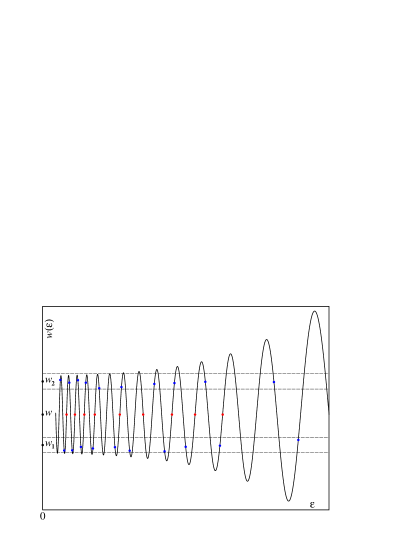
Figure 1: A sketch of behaviour of $w(\varepsilon)$ when two distinct limit weak solutions to the MHD equations coexist (see the text). Points $(\varepsilon_{k,j},w(\varepsilon_{k,j}))$ (blue dots) tend to $(0,w_{k})$ (black dots) for $j\to\infty$, $k=1,2$. The sequence $(\varepsilon_{3,j},w(\varepsilon_{3,j}))\to(0,w)$ (red dots), where $w(\varepsilon_{3,j})=w$, exists due to continuity of $w(\varepsilon)$ in $\varepsilon$ for $\varepsilon>0$. Dashed lines: boundaries of the regions $|w-w_{k}|\leq\gamma$.

References

References

- (1) Adams R.A., Fournier J.J.F. Sobolev spaces. Elsevier, Amsterdam, 2nd ed., 2003.
- (2) Bartuccelli M.V., Doering C.R., Gibbon J.D., Malham S.J.A. Length scales in solutions of the Navier–Stokes equations. Nonlinearity, 6, 549–568 (1993).
- (3) Bergh J., Löfström J. Interpolation spaces. An introduction. Springer, Berlin (1976).
- (4) Biswas A., Foias C. On the maximal space analyticity radius for the 3D Navier–Stokes equations and energy cascades. Annali di Matematica, 193, 739–777 (2014).
- (5) Biswas A., Jolly M.S., Martinez V.R., Titi E.S. Dissipation length scale estimates for turbulent flows: A Wiener algebra approach. J. Nonlinear Sci., 24, 441–471 (2014).
- (6) Bradshaw Z., Grujić Z., Kukavica I. Analyticity radii and the Navier–Stokes equations: recent results and applications. In Recent progress in the theory of the Euler and Navier–Stokes equations. Eds. J.C. Robinson, J.L. Rodrigo, W. Sadowski, A. Vidal-López. CUP, 22–36, 2016.
- (7) Caffarelli L., Kohn R., Nirenberg L. Partial regularity of suitable weak solutions of the Navier–Stokes equations. Comm. Pure Appl. Math., 35, 771–931 (1982).
- (8) Chae D., Chae D. Remarks on the regularity of weak solutions of the Navier–Stokes equations. Comm. Partial Diff. Equations, 17, 359–369 (1992).
- (9) Doering C.R., Gibbon J.D. Applied analysis of the Navier–Stokes equations. CUP, 1995.
- (10) Doering C.R., Titi E.S. Exponential decay rate of the power spectrum for solutions of the Navier–Stokes equations. Phys. Fluids, 7, 1384–1390 (1995).
- (11) Donzis D.A., Gibbon J.D., Gupta A., Kerr R.M., Pandit R., Vincenzi D. Vorticity moments in four numerical simulations of the 3D Navier–Stokes equations. J. Fluid Mech., 732, 316–331 (2013).
- (12) Duvaut G., Lions J.L. Inéquations en thérmoelasticité et magnétohydrodynamique. Arch. Rat. Mech. Anal., 46, 241–279 (1972).
- (13) Escauriaza L., Seregin G.A., Šverák V. -solutions of Navier–Stokes equations and backward uniqueness. Russ. Math. Surv. 58, 211–250 (2003). Transl. from Usp. Mat. Nauk, 58, 3–44 (2003).
- (14) Foias C., Guillopé C., Temam R. New a priori estimates for Navier–Stokes equations in dimension 3. Comm. Partial Diff. Equations, 6, 329–359 (1981).
- (15) Foias C., Manley O., Rosa R., Temam R. Navier–Stokes equations and turbulence (Encyclopedia of mathematics and its applications, 83). CUP, 2001.
- (16) Foias C., Temam R. Determination of the solutions of the Navier–Stokes equations by a set of nodal values. Mathematics of Computation, 43, 117–133 (1984).
- (17) Foias C., Temam R. Gevrey class regularity for the solutions of the Navier–Stokes equations. J. Funct. Anal., 87, 359–369 (1989).
- (18) Frisch U., Zheligovsky V. A very smooth ride in a rough sea. Comm. Math. Phys., 326, 499–505 (2014) [arxiv.org/abs/1212.4333].
- (19) Gibbon J.D. Derivation of 3d Navier–Stokes length scales from a result of Foias, Guillopé and Temam. Nonlinearity, 7, 245–252 (1994).
- (20) Gibbon J.D. A voyage around the Navier–Stokes equations. Physica D, 92, 133–139 (1996).
- (21) Gibbon J.D. Regularity and singularity in solutions of the three-dimensional Navier–Stokes equations. Proc. R. Soc. A, 466, 2587–2604 (2010).
- (22) Gibbon J.D. Weak and strong solutions of the 3D Navier–Stokes equations and their relation to a chessboard of convergent inverse length scales. J. Nonlin. Sci., 29, 215–228 (2019).
- (23) Golovkin K.K., Ladyzhenskaya O.A. Solutions of non-stationary boundary value problems for Navier–Stokes equations. Trudy Mat. Inst. Steklov, 59, 100–114 (1960).
- (24) Hopf E. Über die Anfangswertaufgabe für die hydrodynamischen Grundgleichungen. Math. Nachr., 4, 213–231 (1951).
- (25) Kim S. Gevrey class regularity of the magnetohydrodynamics equations. ANZIAM J., 43, 397–408 (2002).
- (26) Kiselev A., Ladyzhenskaya O. On the existence and uniqueness of the solution of the nonstationary problem for a viscous, incompressible fluid. Izv. Akad. Nauk SSSR. Ser. Mat., 21 (5), 655–680 (1957).
- (27) Ladyzhenskaya O.A. The mathematical theory of viscous incompressible flow. Gordon and Breach, NY, 1969; Nauka, Moscow, 1970, 2nd ed. (in Russian).
- (28) Leray J. Essai sur le mouvement d’un liquide visqueux emplissant l’espace. Acta Math., 63, 193–248 (1934).
- (29) Levermore C.D., Oliver M. Analyticity of solutions for a generalized Euler equation. J. Diff. Equations, 133, 321–339 (1997).
- (30) Lions J.L. Quelque méthodes de résolution des problèmes aux limites non linéaires. Dunod, Paris (1969).
- (31) Maz’ja V.G. Sobolev Spaces. Springer Series in Soviet Mathematics. Springer-Verlag, 1985.
- (32) Oliver M., Titi E.S. Remark on the rate of decay of higher order derivatives for solutions to the Navier–Stokes equations in . J. Functional Analysis, 172, 1–18 (2000).
- (33) Peetre J. Espaces d’interpolation et théorème de Sobolev. Ann. Inst. Fourier, 16, 279–317 (1966).
- (34) Prodi G. Un teorema di unicità per le equazioni di Navier–Stokes. Ann. Mat. Pura Appl., 48, ser. IV, 173–182 (1959).
- (35) Robinson J.C. The Navier–Stokes regularity problem. Phil. Trans. R. Soc. A, 378, 20190526 (2020).
- (36) Robinson J.C., Rodrigo J.L., Sadowski W. The three-dimensional Navier–Stokes equations. Cambridge Studies in Advanced Mathematics, 157. CUP, 2016.
- (37) Scheffer V. Turbulence and Hausdorff dimension. In Turbulence and the Navier–Stokes equations. Lecture Notes in Math., 565. Ed. R. Temam. Springer-Verlag, 94–112 (1976).
- (38) Scheffer V. Partial regularity of solutions to the Navier–Stokes equations. Pacific J. Math., 66, 535–552 (1976).
- (39) Scheffer V. Hausdorff measure and the Navier–Stokes equations. Comm. Math. Phys., 55, 97–112 (1977).
- (40) Scheffer V. The Navier–Stokes equations on a bounded domain. Comm. Math. Phys., 73, 1–42 (1980).
- (41) Sermange M., Temam R. Some mathematical questions related to the MHD equations. Comm. Pure Appl. Math., 36, 635–664 (1983).
- (42) Serrin J. On the interior regularity of weak solutions of the Navier–Stokes equations. Arch. Rational Mech. Anal., 9, 187–195 (1962).
- (43) Solonnikov V.A. Estimates for solutions of a non-stationary linearized system of Navier–Stokes equations. Trudy Mat. Inst. Steklov, 70, 213–317 (1964).
- (44) Tartar L. Topics in nonlinear analysis. Publications Mathématiques d’Orsay, Université Paris-Sud, Orsay (1978).
- (45) Temam R. Navier–Stokes equations and nonlinear functional analysis. SIAM, Philadelphia. 2nd ed., 1983.
- (46) Triebel H. Interpolation theory. Function spaces. Differential operators. VEB Deutscher Verlag der Wissenschaften, Berlin, 1978.
- (47) Weir A.J. Lebesgue integration and measure. CUP, 1973.
- (48) Zheligovsky V. A priori bounds for Gevrey–Sobolev norms of space-periodic three-dimensional solutions to equations of hydrodynamic type. Advances in differential equations, 16, 955–976 (2011) [arxiv.org/abs/1001.4237].
- (49) Zheligovsky V., Frisch U. Time-analyticity of Lagrangian particle trajectories in ideal fluid flow. J. Fluid Mech., 749, 404–430 (2014) [arxiv.org/abs/1312.6320].