Link Quality-Guaranteed Minimum-Cost Millimeter-Wave Base Station Deployment

Abstract

Today’s growth in the volume of wireless devices coupled with the promise of supporting data-intensive 5G-&-beyond use cases is driving the industry to deploy more millimeter-wave (mmWave) base stations (BSs). Although mmWave cellular systems can carry a larger volume of traffic, dense deployment, in turn, increases the BS installation and maintenance cost, which has been largely ignored in their utilization. In this paper, we present an approach to the problem of mmWave BS deployment in urban environments by minimizing BS deployment cost subject to BS association and user equipment (UE) outage constraints. By exploiting the macro diversity, which enables each UE to be associated with multiple BSs, we derive an expression for UE outage that integrates physical blockage, UE access-limited blockage, and signal-to-interference-plus-noise-ratio (SINR) outage into its expression. The minimum-cost BS deployment problem is then formulated as integer non-linear programming (INP). The combinatorial nature of the problem motivates the pursuit of the optimal solution by decomposing the original problem into the two separable subproblems, i.e., cell coverage optimization and minimum subset selection subproblems. We provide the optimal solution and theoretical justifications of each subproblem. The simulation results demonstrating UE outage guarantees of the proposed method are presented. Interestingly, the proposed method produces a unique distribution of the macro-diversity orders over the network that is distinct from other benchmarks.

I Introduction

Communications in the millimeter-wave (mmWave) bands will play a crucial role in facilitating the data-intensive fifth-generation (5G) use cases, including real-time machine-type communications (MTC), interactive on-line learning, and augmented reality (AR) streaming. The potential of the mmWave band has made it as one of the important aspects of future cellular networks [1, 2, 3]. While it is true that mmWave bands provide very high rate connectivity, contrary to general belief, this does not necessarily translate to high achievable throughput due to significant differences between systems operating in mmWave and legacy sub-$6$GHz bands.

I-A MmWave Channel Access Challenges

The initial channel access in the mmWave cellular environment is a very critical problem, especially, using directional analog-digital beamforming [4, 5, 6, 7, 8, 9]. The reliable user equipment (UE) access is critically limited by physical blockage and UE-access saturation in dense urban environments. Specifically, weak diffraction and penetration due to the high pathloss in mmWave bands make channels susceptible to physical blockage by random obstacles [10, 11]. If the channel does not experience physical blockage, the UE can attempt channel access to BS. However, the number of concurrently served UEs by a BS, which is equipped with hybrid analog-digital multiple-input multiple-output (MIMO) arrays, is strictly limited by the number of available radio frequency (RF) chains [4, 5, 6, 7, 8, 9]. When the number of active UEs in a cell is larger than the number of RF chains, UE access-limited blockage occurs. Even without the physical and UE access-limited blockages, accumulated interference from surrounding mmWave small-cells can potentially lower the signal-to-interference-plus-noise ratio (SINR) of each UE, causing SINR outage [12]. Both physical and UE access-limited blockages, as well as the SINR outage, will lead to an unsatisfactory user experience.

Recently, the physical blockage challenge has been addressed by introducing macro diversity [13, 14, 15] that allows for each UE in an area to be covered by multiple BSs. Provided macro diversity, if a link of a UE is blocked, the link can be restored by another BS that also covers the UE. However, this benefit comes at the price of the growing number of deployed BSs. The recent increase in the cost of deploying and maintaining small-cell BSs is a practical concern that wireless service providers are constantly facing [16].

I-B Related Work

An efficient strategy for BS deployment is minimizing the number of deployed BSs subject to per-UE quality constraints. In this category, BS density optimization [17, 18, 19, 20, 21, 22] and site-specific BS deployment [23, 24, 25, 26] methods have been previously studied. The BS density optimization methods [17, 18, 19, 20, 21, 22] rely on stochastic geometry to find minimum BS density subject to cell coverage constraints. While these prior works [17, 18, 19, 20, 21, 22] provide theoretical insights into the distribution of BSs, they rather fit traditional macro-cellular environments. In the context of small-cell, the site-specific BS deployment methods [23, 24, 25, 26] have been studied, which find the minimum number of BSs installed on predetermined candidate locations. The underlying assumption of these works was omnidirectional and penetrable wave propagation in the sub-$6$GHz bands, which cannot be extended to mmWave.

Incorporating mmWave pathloss models, site-specific BS deployment techniques have been studied to maximize line-of-sight (LoS) link distance given a fixed number of BSs [27, 28, 29, 30]. While the works in [27, 28, 29, 30] considered general urban geometry, the work in [31] focused on a specific Manhattan-type geometry to maximize the macro diversity. Recently, the minimum-number BS deployment problem has been studied for guaranteeing the average receive signal power [32], link-blockage tolerance level [33], and beam alignment reliability due to random UE rotation [34]. Unlike the prior works [27, 28, 29, 30, 32, 34], the methodologies in [33, 31] integrate the mmWave physical blockage and UE access-limited blockage models into their problem formulations. However, these works either are limited to a specific Manhattan-type geometry [31] or ignore important link-quality measures [33, 31], such as SINR that must be taken in when designing and evaluating the performance of a BS deployment method. Thus, it is of great interest to develop a rather pragmatic strategy that accounts for various mmWave-link-quality-related constraints. Such approaches must be flexible to be applicable to any urban geometry and can incorporate both the installation cost and the number of BSs into its objective [16].

In this paper, we consolidate the latter missing components and formulate the BS deployment problem into integer nonlinear programming (INP). About existing work, this aspect has some similarities to the well-investigated problems on optimizing BS sleeping and user association at sub-$6$GHz bands. The latter problems were often addressed by formulating INP with the objectives of maximizing network throughput [35, 36] or minimizing the power consumption [24, 25, 26, 37, 38]. Because large-scale INP is NP-hard and is generally very difficult to be optimally solved, devising suboptimal but efficient algorithms was the focus of these approaches, by using greedy heuristics [26, 25, 24], Lagrangian dual [38, 36], and sequential subproblem formulations [37, 35]. Though these subproblem frameworks were largely benefited from the deterministic link models at sub-$6$GHz bands, such models and associated problem formulations cannot be extended to the mmWave. Although prior approaches [26, 25, 24, 37, 35, 38, 36] deal with INP, they are different from our proposed approach in terms of the objective functions, associated constraints, and thereby, the developed algorithms.

I-C Overview of Methodology and Contributions

We address important mmWave connectivity challenges in a 3-dimensional (3D) urban geometry by proposing a link quality-guaranteed minimum-cost mmWave BS deployment technique. Our contributions are summarized below.

• We introduce a mmWave link state model that captures the randomness of physical blockage, UE access-limited blockage, and SINR outage events. The model accounts for random locations of UEs and obstacles in stochastic geometry, which allows us to mathematically formulate the UE outage and BS association constraints. However, these expressions are not analyzable and difficult to be used for formulating optimization problems. We show instead that the UE outage constraint can be upper bounded to derive a tractable expression. Moreover, we verify that the UE access-limited blockage constraint can be equivalently transformed to an analytic (linear) model, facilitating a tractable optimization framework.

• Next, we present the minimum-cost mmWave BS deployment problem as large-scale INP. However, the formulated INP is difficult to be solved directly. While this could motivate us to pursue suboptimal algorithms (e.g., [26, 25, 24, 38, 36, 37, 35, 32, 33]), we instead show that the formulated INP can be decomposed into two separable subproblems, i.e., (i) cell coverage optimization problem and (ii) minimum subset BS selection problem, and optimally solved by sequentially solving these two subproblems. In particular, we show that the second subproblem (minimum subset BS selection problem), which is also INP, can be transformed into a linear equivalent form that can be efficiently solved via existing software.

• Finally, we evaluate the performance of our proposed designs via numerical results. We show that the proposed scheme provides UE outage guarantees with the minimum-cost BS deployment, in contrast to other benchmark schemes [32, 34]. An interesting aspect of the proposed scheme is that the optimized results present a unique distribution of the macro-diversity orders over the network that lowers the concentration of macro-diversity orders compared to other benchmark schemes in [32, 34]. This is the underlying reason of the improved performance guarantee compared to the benchmarks, while deploying a reduced number of BSs.

The rest of the paper is organized as follows. We present the system models in Section II. The UE outage-guaranteed minimum-cost mmWave BS deployment problem is formulated in Section III. The proposed algorithm that solves the problem is enunciated in Section IV. The simulation results and conclusions are provided in Section V and VI, respectively. For ease of reference, TABLE I summarizes the main variables which will be used throughout this paper.

II System Models

In this section, we provide a mathematical description for the mmWave cellular environment and system model under consideration.

TABLE I: List of Main Variables and Their Physical Meanings

Variable	Description
$G_{\text{main}}$	Mainlobe beam gain
$G_{\text{side}}$	Sidelobe beam gain
$H_{\text{BS},b}$	Height of BS $b$
$H_{\text{UE}}$	Height of UEs
$I_{i,g}$	Interference power from BS $i$ to UE $g$
$L_{\text{grd}}$	Length of square grid
${n}_{b}\left({\mathbf{x}}_{b}\right)$	Number of active UEs in cell $b$ with area $\sum_{g}\!x_{b,g}L_{\text{grd}}^{2}$
$N_{\text{RF}}$	Number of RF chains at each BS
$P_{b,g}$	Transmit power of link from BS $b$ to UE $g$
$p_{b,g}^{\text{blk}}$	Physical blockage probability of link from BS $b$ to UE $g$
$p_{b,g}^{\text{out}}$	Outage probability of link from BS $b$ to UE $g$
$\text{PL}_{b,g}$	Pathloss of the link from BS $b$ to grid $g$
$R^{\text{max}}$	Maximum allowed link distance for reliable communications
$r_{b,g}$	Distance of the link from BS $b$ to grid $g$
$r_{b}^{\text{max}}$	Maximum link distace in cell $b$
$\text{SINR}_{b,g}$	SINR of link from BS $i$ to UE $g$
$\mathbf{X}\!\in\!\mathbb{B}^{B\!\times\!G}$	Association matrix
$\mathbf{x}_{b}\!\in\!\mathbb{B}^{1\!\times\!G}$	The $b$th row of $\mathbf{X}$
$\mathbf{y}\!\in\!\mathbb{B}^{1\!\times\!B}$	BS deployment vector
$z$	SINR threshold
$\lambda_{\text{UE},g}$	UE density in grid $g$,
$\zeta$	UE outage tolerance
$\gamma$	UE access-limited blockage tolerance
$\sigma^{2}$	Noise power

II-A Urban Geometry

We consider a 3D urban geometry, for example, as illustrated in Fig. 1, consisting of buildings and streets. In Fig. 1, mmWave BSs are mounted on walls of the buildings to serve outdoor active UEs on the streets in the downlink. We assume that the candidate BS locations are predetermined as red dots in Fig. 1 and let the indices of the candidate BS locations be $\mathcal{B}\!=\!\{1,2,\ldots,B\}$. Each candidate location has the height $H_{\text{BS},b},\forall b\in\mathcal{B}$. If a BS is installed at the $b$th ($b\in{\mathcal{B}}$) location, $y_{b}=1$ and otherwise, $y_{b}=0$, where $y_{b}\in\mathbb{B}=\{0,1\}$ is the $b$th entry of the BS deployment vector $\mathbf{y}=[y_{1},\ldots,y_{B}]\in{\mathbb{B}}^{1\times B}$. Hereafter, a BS deployed at the $b$th candidate location is called “BS $b$”.

Each mmWave BS has its coverage area, called a cell. Each BS serves outdoor active UEs inside its cell. Due to the physical blockage by obstacles and buildings, the shape of a cell is irregular. In our approach, to capture the irregularity of each cell, the whole outdoor area is divided into $G$ square grids in Fig. 1. The location of each grid is represented by its center point. We let the index set of the grids be $\mathcal{G}\!=\!\{1,2,\ldots,G\}$. For simplicity, we call a UE in grid $g$ as “UE $g$”. An association indicator $x_{b,g}\in{\mathbb{B}}$ is introduced, where $x_{b,g}\!=\!1$ if the grid $g\in{\mathcal{G}}$ resides in the cell of BS $b$, and $x_{b,g}=0$, otherwise. The cell area associated with BS $b$ then equals to $\sum_{g}x_{b,g}L_{\text{grd}}^{2}$, where $L_{\text{grd}}$ is the length of the side of a square grid in Fig. 1. The overlap between cells is allowed so that some UEs in a cell can be simultaneously covered by more than one BS (i.e., macro diversity)

$$\sum_{b\in{\mathcal{B}}}x_{b,g}\geq 1.$$ (1)

All association indicators $\{x_{b,g}\}$ are collected into an association matrix $\mathbf{X}\in\mathbb{B}^{B\times G}$, where its $b$th row and $g$th column entry is $x_{b,g}$. We assume that UEs have the same height $H_{\text{UE}}$ and $H_{\text{UE}}\!<\!H_{\text{BS},b},\forall b\in\mathcal{B}$. UEs in the outdoor area are randomly distributed and their placements can be accurately modeled by a non-homogeneous Poisson point process (PPP) with a certain UE density distribution [39, 40]. For ease of exposition, when the partitioned square grid in Fig. 1 is small enough, we assume that the users in a grid $g$ are uniformly distributed with a density $\lambda_{\text{UE},g}$, $g\!\in\!{\mathcal{G}}$. The different grid can have different UE density $\lambda_{\text{UE},g}$. This approximation becomes exact as the square grid reduces to a point.

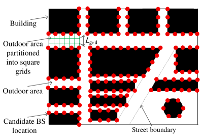
Figure 1: Bird’s-eye view of an exemplary urban street geometry for mmWave BS deployment.

II-B Pathloss Model

MmWave propagation experiencing severe pathloss and atmospheric impairments exhibits sparse multi-path channels. In particular, weak diffraction and penetration at mmWave frequencies make the non-LoS (NLoS) paths suffer from much severer attenuation than the LoS paths. As a result, the quality of a mmWave link is dominantly determined by its LoS link [41]. Hence, in this work, we mainly focus on the LoS path. In the recent 3GPP specifications (Release 15 [42]), the $28$ GHz mmWave band has been considered as one of the standard frequencies for 5G cellular communications. Throughout the paper, we will use the $28$ GHz LoS pathloss model based on the measurement campaign conducted in an urban area [10], which is characterized by

$$\text{PL}_{b,g}=10^{-3.24-2.1\cdot\mathrm{log}_{10}(r_{b,g})-2.0\cdot\mathrm{log}_{10}(28)},$$ (2)

where $\text{PL}_{b,g}$ is the pathloss from BS $b$ to a UE $g$, and $r_{b,g}$ is the link distance in meters. We assume that the link distance $r_{b,g}$ is limited by a constant $R^{\text{max}}$, $r_{b,g}\leq R^{\text{max}}$, where $R^{\text{max}}$ is the maximum allowed mmWave link distance for reliable communications. Thus, we assume any link with the distance $r_{b,g}>R^{\text{max}}$ is in outage.

II-C Hybrid Array and Beam Pattern

II-C1 Hybrid Analog-Digital Arrays

The mmWave frequencies force systems to use large-sized antenna arrays to generate highly directional narrow beams in order to overcome the propagation impairments [1]. To make the large-sized arrays available at low cost, analog arrays that are driven by a limited number ($N_{\text{RF}}$) of RF chains are typically employed. This system is referred to as a hybrid analog-digital mmWave MIMO system [4, 5, 6, 7, 8, 9], which is the major realization technology of 5G mmWave BS systems. Throughout the paper, we assume such hybrid mmWave MIMO BS systems.

II-C2 Beam Pattern

For ease of exposition, we assume a simplified directional beam pattern, also called the cone-shaped beam pattern, at BSs as follows

$$\small\textstyle{G_{\text{BS}}(\theta,\phi)\!=\!}\textstyle\left\{\begin{array}[]{ll}\textstyle\!\!\!G_{\text{main}},\!&\text{if}\;|\theta|\leq\frac{\Delta_{\theta}}{2},\;|\phi|\leq\frac{\Delta_{\phi}}{2}\\ \!\!\!G_{\text{side}},\!\!&\textstyle\text{otherwise}\end{array},\right.$$ (3)

where $G_{\text{main}}$ and $G_{\text{side}}$ are the array gains at the mainlode and sidelobe, respectively. Then, $G_{\text{BS}}(\theta,\phi)$ represents the beam gain at elevation $\theta$ and azimuth $\phi$ directions. The $\Delta_{\theta}$ and $\Delta_{\phi}$ in (3) are, respectively, the beamwidths at the elevation $\theta$ and azimuth $\phi$ directions. Though model (3) is an approximation, it can be shown that (3) closely approach to the actual beam pattern as the array size increases [12, 44, 45]. The BS aligns its beam to provide beamforming gain $G_{\text{main}}$ to a UE. In this work, we assume a single antenna UE that generates an omnidirectional receive beam.

III Link Analysis and Problem Formulation

In this section, we identify several key constraints and the statistics of elementary events, including the physical blockage probability, BS association constraints, UE access-limited blockage probability, and SINR outage probability that are used to formulate the UE outage constraint. These are then combined to define the mmWave BS deployment problem at the end of this section.

III-A Physical Blockage Probability

The physical blockage of mmWave links depends not only on the distance of a link, but also on the density and sizes of random obstacles [46, 12]. The random obstacles are assumed to be impenetrable cubes, based on the Boolean scheme, and the placement of each obstacle follows a homogeneous PPP with the density $\lambda_{\text{obs}}$ [11]. The physical blockage probability with the path length $r_{b,g}$ is then given by

$$\!\!\!\!p_{b,g}^{\text{blk}}\!=\!\textstyle\!\left\{\begin{array}[]{ll}\textstyle\!\!1\!-\!\mathrm{exp}(-\beta r_{b,g}\!-\!\alpha)\!\!\!\!\!&,~{}\text{if $\exists$ LoS path}\\ \!\!1\!\!\!&,~{}\textstyle\text{otherwise}\end{array},\right.$$ (4)

where $r_{b,g}\leq R^{\text{max}}$ and $\alpha$ and $\beta$ are parameters that depend on the density and sizes of the obstacles [11]. The variables in (4) follow $\beta\!=\!2\lambda_{\text{obs}}\frac{E[L_{\text{obs}}]+E[W_{\text{obs}}]}{\pi}\eta$ and $\alpha=\lambda_{\text{obs}}E[L_{\text{obs}}]E[W_{\text{obs}}]$, where $E[L_{\text{obs}}]$ and $E[W_{\text{obs}}]$ are the expected length and width of obstacles, respectively, and $\eta=1\!-\!\int_{0}^{1}\int_{0}^{sH_{\text{UE}}+(1-s)H_{\text{BS}}}f_{h}(x)dxds$ where $f_{h}(x)$ is the probability density function of the height of an obstacle. The intuition behind (4) is that the denser the obstacle distribution and the larger the obstacle sizes, the larger $\alpha$ and $\beta$ values will be, resulting in a higher blockage probability.

III-B BS Association Constraints

In this subsection, we list the rules for elements in the association matrix ${\mathbf{X}}$. These elements will be used for formulating the UE access-limited blockage and SINR outage probabilities in the next two subsections.

If a BS is installed at the $b$th candidate location ($y_{b}\!=\!1$), the association variable is either $x_{b,g}=1$ or $x_{b,g}=0$, while if $y_{b}\!=\!0$, then $x_{b,g}\!=\!0$, yielding

$$x_{b,g}\leq y_{b},\quad b\in\mathcal{B},\;g\in\mathcal{G}.$$ (5)

Based on the physical blockage model in the previous subsection, it is evident that necessary conditions for $x_{b,g}=1$ are: (i) the link distance $r_{b,g}\leq R^{\text{max}}$ and (ii) the physical blockage probability $p_{b,g}^{\text{blk}}<1$ in (4), which leads to

$$x_{b,g}\leq\mathbb{I}_{\left\{{{r_{b,g}\leq R^{\text{max}},\;p_{b,g}^{\text{blk}}}<1}\right\}},\;b\in\mathcal{B},g\in\mathcal{G},$$ (6)

where $\mathbb{I}_{\left\{{\mathcal{A}}\right\}}$ is an indicator function: $\mathbb{I}_{\left\{{\mathcal{A}}\right\}}=1$ if the event ${\mathcal{A}}$ is true, and $\mathbb{I}_{\left\{{\mathcal{A}}\right\}}=0$ otherwise. We assume that the grids closer to a BS have the priority to be associated with the BS. This is to say, whenever a grid $g$ is served by BS $b$ ($x_{b,g}=1$), other grid $s\in{\mathcal{G}}$ with $r_{b,s}\leq r_{b,g}$ and $p_{b,s}^{\text{blk}}<1$ should also be served by the BS $b$, leading to

$$\mathbb{I}_{\left\{{{r_{b,s}\leq r_{b,g},\;p_{b,s}^{\text{blk}}}<1}\right\}}x_{b,g}\leq x_{b,s},\;b\in\mathcal{B},g,s\in\mathcal{G}.$$ (7)

The conditions in (5), (6), and (7) will be incorporated in our proposed BS deployment problem as the BS association constraints.

III-C UE Access-Limited Blockage Probability

When the mmWave channel between a UE and BS does not experience physical blockage, the UE can attempt channel access to the BS. However, it can still be blocked due to saturated UE access within a cell. More specifically, the maximum number of UEs that a BS can simultaneously serve is strictly limited by the number of RF chains $N_{\text{RF}}$ in hybrid MIMO BS systems. UE access-limited blockage occurs whenever the number of active UEs in a cell is larger than $N_{\text{RF}}$. This blockage has an intuitive interrelation between the UE density $\lambda_{\text{UE},g}$ and the number of grids covered by a BS $\sum_{g}x_{b,g}$. For instance, if a BS covers a larger number of grids, it results in a higher probability of UE access-limited blockage. The same is true when the UE density per grid $\lambda_{\text{UE},g}$ grows. To capture this interrelation and to use it for controlling the numbers of grids covered by BSs, we now derive the UE access-limited blockage probability between BS $b$ and a UE in grid $g$ denoted by $\rho_{b,g}({\mathbf{x}}_{b})$, where ${\mathbf{x}}_{b}=[x_{b,1},\ldots,x_{b,G}]\in{\mathbb{B}}^{1\times B}$ is the $b$th row of the association matrix ${\mathbf{X}}$.

We let ${n}_{b}\left({\mathbf{x}}_{b}\right)$ be the number of active UEs without physical blockage in the cell area $\sum_{g}\!x_{b,g}L_{\text{grd}}^{2}$ of BS $b$. Then, the UE access-limited blockage at BS $b$ occurs when ${n}_{b}\left({\mathbf{x}}_{b}\right)>N_{\text{RF}}$, in which ${n}_{b}\left({\mathbf{x}}_{b}\right)$ is a random variable that depends on UE distribution and random physical blockage. Assume that each of the ${n}_{b}\left({\mathbf{x}}_{b}\right)$ UEs has the equal probability to have successful channel access without UE access-limited blockage. For a given ${n}_{b}\left({\mathbf{x}}_{b}\right)$ with ${n}_{b}\left({\mathbf{x}}_{b}\right)>N_{\text{RF}}$, the UE $g$ is then in UE access-limited blockage with probability

$$\frac{{n}_{b}\left({\mathbf{x}}_{b}\right)-N_{\text{RF}}}{{n}_{b}\left({\mathbf{x}}_{b}\right)}.$$

The UE access-limited blockage probability $\rho_{b,g}({\mathbf{x}}_{b})$ is therefore given by

$$\rho_{b,g}({\mathbf{x}}_{b})=\sum\limits_{\forall x\;\text{with}\;x>N_{\text{RF}}}\Pr({n}_{b}\left({\mathbf{x}}_{b}\right)=x)\frac{x-N_{\text{RF}}}{x}$$ (8)

Identifying $\Pr({n}_{b}\left({\mathbf{x}}_{b}\right)=x)$ in (8) requires the distribution of $n_{b}(\mathbf{{\mathbf{x}}_{b}})$. By leveraging the independent thinning property of PPP [47], the number of active UEs, associated with BS $b$, without physical blockage per grid $g$ is Poisson distributed with the mean $\lambda_{\text{UE},g}L^{2}_{\text{grd}}(1-p_{b,g}^{\text{blk}}).$ Because the sum of independent Poisson random variables is still Poisson, ${n}_{b}({\mathbf{x}}_{b})$ is Poission-distributed with the mean

$$E[{n}_{b}({\mathbf{x}}_{b})]=\sum_{g\in\mathcal{G}}x_{b,g}\lambda_{\text{UE},g}L^{2}_{\text{grd}}(1-p_{b,g}^{\text{blk}}).$$ (9)

The closed-form expression of (8) is therefore given by

$$\rho_{b,g}({\mathbf{x}}_{b})\!=\!\sum_{i=N_{\text{RF}}+1}^{+\infty}\!\!\frac{E[{n}_{b}({\mathbf{x}}_{b})]^{i}}{i!}e^{-E[{n}_{b}({\mathbf{x}}_{b})]}\frac{i-N_{\text{RF}}}{i}.$$ (10)

The following lemma characterizes the relationship between the UE access-limited blockage probability in (10) and the cell coverage and UE density.

Lemma 1.

The UE access-limited blockage probability $\rho_{b,g}({\mathbf{x}}_{b})$ in (10) is a monotonically increasing function of the cell coverage (i.e., $\sum_{g}x_{b,g}$) and/or UE density $\lambda_{\text{UE},g}$.

Proof.

It is not difficult to observe from (9) that $E[{n}_{b}({\mathbf{x}}_{b})]$ increases as the $\sum_{g}x_{b,g}$ and/or UE density $\lambda_{\text{UE},g}$ grow. Hence, the proof of the lemma boils down to showing that the $\rho_{b,g}$ in (10) is a monotonically increasing function of $E[{n}_{b}({\mathbf{x}}_{b})]$. This can be verified by taking the first-order derivative of $\rho_{b,g}({\mathbf{x}}_{b})$ with respect to $E[{n}_{b}({\mathbf{x}}_{b})]$, yielding

$$\textstyle\frac{\partial\rho_{b,g}({\mathbf{x}}_{b})}{\partial E[{n}_{b}(\mathbf{x}_{b})]}\!\!\!\!\!\! \!=\! \!\!\!\!\!\!\textstyle\sum\limits_{i=N_{\text{RF}}+1}^{+\infty}\frac{E[{n}_{b}(\mathbf{x}_{b})]^{i-1}}{(i-1)!}e^{-E[{n}_{b}(\mathbf{x}_{b})]}\frac{i-N_{\text{RF}}}{i}$$

$$\!\!\!\!\hskip 28.45274pt-\!\textstyle\sum\limits_{i=N_{\text{RF}}+1}^{+\infty}\frac{E[{n}_{b}(\mathbf{x}_{b})]^{i}}{i!}e^{-E[{n}_{b}(\mathbf{x}_{b})]}\frac{i-N_{\text{RF}}}{i}$$

$$\stackrel{{\scriptstyle(a)}}{{\!=\!}} \!\!\!\!\!\!\textstyle e^{-E[{n}_{b}(\mathbf{x}_{b})]}\!\!\left(\!\!\frac{E[{n}_{b}(\mathbf{x}_{b})]^{N_{\text{RF}}}}{(N_{\text{RF}}+1)!}\!+\!\!\!\!\!\!\!\sum\limits_{i=N_{\text{RF}}+1}^{+\infty}\!\!\!\!\!\!\frac{E[{n}_{b}(\mathbf{x}_{b})]^{i}}{i!}\!\left(\!\frac{N_{\text{RF}}}{i}\!\!-\!\!\frac{N_{\text{RF}}}{i+1}\!\right)\!\!\right)\;\;$$

$$\geq 0,$$

where the step (a) follows from the fact that $\sum\limits_{i=N_{\text{RF}}+1}^{+\infty}\!\!\!\!\frac{E[{n}_{b}(\mathbf{x}_{b})]^{i-1}}{(i-1)!}e^{-E[{n}_{b}(\mathbf{x}_{b})]}\frac{i-N_{\text{RF}}}{i}$ in the first equality can be rewritten as

$$\textstyle e^{-E[{n}_{b}(\mathbf{x}_{b})]}\frac{E[{n}_{b}(\mathbf{x}_{b})]^{N_{\text{RF}}}}{(N_{\text{RF}}+1)!}+\!\!\sum\limits_{i=N_{\text{RF}}+1}^{+\infty}\!\frac{E[{n}_{b}(\mathbf{x}_{b})]^{i}}{i!}e^{-E[{n}_{b}(\mathbf{x}_{b})]}\frac{i+1-N_{\text{RF}}}{i+1}.$$

This completes the proof. ∎

III-D SINR Outage Probability

While a UE that does not experience physical and UE access-limited blockages can acquire initial access to BS, the acquired link can be unavailable due to intercell and intracell interference from surrounding BSs. Hence, describing the SINR outage $\Pr\left(\text{SINR}_{b,g}({\mathbf{y}},{\mathbf{X}})\!<\!z|\mathbf{y},\mathbf{X}\!\right)$, where $\text{SINR}_{b,g}({\mathbf{y}},{\mathbf{X}})$ is the SINR of a link from BS $b$ to a UE $g$ and $z$ is the SINR threshold for reliable communications, is of interest. Directly analyzing the distribution of $\text{SINR}_{b,g}(\mathbf{y},\mathbf{X})$ in the mmWave environment is very difficult due to stochastic physical blockage and UE distribution. In this subsection, we resort to a deterministic lower bound of $\text{SINR}_{b,g}$ to propose a closed-form approximate of $\Pr\left(\text{SINR}_{b,g}({\mathbf{y}},{\mathbf{X}})<z|\mathbf{y},\mathbf{X}\right)$.

We assume an equal power allocation per UE and write the desired signal power $P_{b,g}(\mathbf{x}_{b})$ received at an active UE in grid $g$ from its serving BS $b$ as

$$P_{b,g}(\mathbf{x}_{b})\!\!\!\!\!\!\!\! =\frac{x_{b,g}P_{\text{TX}}}{\min(n_{b}({\mathbf{x}}_{b}),N_{\text{RF}})}G_{\text{main}}\text{PL}_{b,g}$$ (11)

$$\geq\frac{x_{b,g}P_{\text{TX}}}{N_{\text{RF}}}G_{\text{main}}\text{PL}_{b,g}\;\triangleq\;\overline{P}_{b,g}(x_{b,g}),$$

where $P_{\text{TX}}$ is the total BS transmit power, $\min(n_{b}({\mathbf{x}}_{b}),N_{\text{RF}})$ is the number of served active UEs by BS $b$, $G_{\text{main}}$ follows (3), and $\text{PL}_{b,g}$ is in (2). The last inequality in (11) is due to $\min(n_{b}({\mathbf{x}}_{b}),N_{\text{RF}})\leq N_{\text{RF}}$. We now capture the composite link interference power under an assumption that the mainlobe of a 3D beam in (3) is perfectly aligned with the intended UE and is narrow enough not to cause interference to unintended UEs. Thus, it is the sidelobe of the beam that causes interference with probability $1$. A BS $i$ serving $\min(n_{i}({\mathbf{x}}_{i}),N_{\text{RF}})$ UEs has in total $\min(n_{i}({\mathbf{x}}_{i}),N_{\text{RF}})$ beams and can possibly impose interference $I_{i,g}(\mathbf{x}_{b})$ to the UE in grid $g$ with $\min(n_{i}({\mathbf{x}}_{i}),N_{\text{RF}})-x_{i,g}$ interfering sidelobes if there exists an LoS path between the BS $i$ and UE $g$. In the case of $p_{i,g}^{\text{blk}}<1$ in (4), the interference $I_{i,g}(\mathbf{x}_{b})$ is a Bernoulli random variable with its value either $0$ (blocked) or positive (unblocked), yielding

$$I_{i,g}(\mathbf{x}_{b})\!\!\!\!\!\!\!\!\!\!\!\! =\!\mathbb{I}_{\left\{{\mathcal{A}}_{i,g}\right\}}\!\frac{\big{(}\!\min(n_{i}({\mathbf{x}}_{i}),N_{\text{RF}})\!-\!x_{i,g}\big{)}P_{\text{TX}}}{\min(n_{i}({\mathbf{x}}_{i}),N_{\text{RF}})}G_{\text{side}}\text{PL}_{i,g}\;\;\quad$$ (12)

$$\leq\!\left(\!1\!-\!\frac{x_{i,g}}{N_{\text{RF}}}\right)P_{\text{TX}}G_{\text{side}}\text{PL}_{i,g}\!\triangleq\!\widehat{I}_{i,g}(x_{i,g}),$$

where ${\mathcal{A}}_{i,g}$ denotes the event that the LoS path between the BS $i$ and UE $g$ is not physically blocked. The last inequality in (12) is due to the facts that $\mathbb{I}_{\left\{{\mathcal{A}}_{i,g}\right\}}\leq 1$ and $\min(n_{i}({\mathbf{x}}_{i}),N_{\text{RF}})\leq N_{\text{RF}}$. When $n_{i}({\mathbf{x}}_{i})=N_{\text{RF}}$, the $\widehat{I}_{i,g}(x_{i,g})$ is the positive value of the Bernoulli random $I_{i,g}(\mathbf{x}_{b})$ and becomes tight if the link is blocked with a low probability. Accounting for (11) and (12), we have the lower bound

$$\text{SINR}_{b,g}(\mathbf{y},\mathbf{X})\geq\overline{\text{SINR}}_{b,g}(\mathbf{y},\mathbf{X})\!=\!\frac{\overline{P}_{b,g}(x_{b,g})}{\sigma^{2}+\sum\limits_{i\in\mathcal{B}}y_{i}\widehat{I}_{i,g}(x_{i,g})},$$ (13)

where the $\sigma^{2}$ is the noise power. The conditional probability of $\overline{\text{SINR}}_{b,g}(\mathbf{y},\mathbf{X})<z$ given $\mathbf{y}$ and $\mathbf{X}$ is therefore given by

$$\Pr\left(\overline{\text{SINR}}_{b,g}(\mathbf{y},\mathbf{X})\!<\!z|\mathbf{y},\mathbf{X}\!\right)={\mathbb{I}}_{\big{\{}\overline{\text{SINR}}_{b,g}(\mathbf{y},\mathbf{X})<z|\mathbf{y},\mathbf{X}\big{\}}},$$ (14)

which is an upper bound of the SINR outage probability

$$\Pr\left({\text{SINR}}_{b,g}(\mathbf{y},\mathbf{X})\!<\!z|\mathbf{y},\mathbf{X}\!\right)\!\!\!\! \leq \!\!\!\!\Pr\left(\overline{\text{SINR}}_{b,g}(\mathbf{y},\mathbf{X})\!<\!z|\mathbf{y},\mathbf{X}\!\right).$$ (15)

Remark 1.

The lower bound in (13) is obtained based on the lower bound of the desired signal power in (11) and the upper bound of the interference power in (12). Note that the bound in (11) becomes tight when $n_{b}({\mathbf{x}}_{b})\approx N_{\text{RF}}$; it indeed becomes the equality when $n_{b}({\mathbf{x}}_{b})=N_{\text{RF}}$. Similarly, the bound in (12) becomes tight when $n_{b}({\mathbf{x}}_{b})\approx N_{\text{RF}}$. It can be further tighten when the accumulated interference $\sum_{i\in\mathcal{B}}y_{i}\widehat{I}_{i,g}(x_{i,g})$ in (13) is dominated by nearby BSs of the grid $g$ because in this case the link distances between the nearby BSs and the grid $g$ are relatively small, resulting in low physical blockage probabilities $p_{i,g}^{\text{blk}}$ and revealing a higher chance for the event ${\mathcal{A}}_{i,g}$ in (12).

III-E UE Outage Constraint

To formulate the UE outage constraint that takes in the physical blockage, UE access-limited blockage, and SINR outage, we first identify the UE outage probability associated with a single link from a BS to a UE. This is then extended to the UE outage constraint that captures the effect of surrounding BSs.

III-E1 Single-Link UE Outage Probability

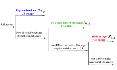
Figure 2: Logical relationship of the three events causing UE outage.

A link from BS $b$ to a UE $g$ is in outage if one of the following mutually exclusive events occurs as described in the previous subsections: (i) Event ${\mathcal{P}}_{b,g}$: the channel is physically blocked; (ii) Event ${\mathcal{U}}_{b,g}$: the channel is physically unblocked, but the UE access-limited blockage occurs; and (iii) Event ${\mathcal{S}}_{b,g}$: the link has no blockage and the UE acquires initial access to BS (i.e., SINR${}_{b,g}\geq 0$), but the SINR outage occurs. The logical relationship of the three events is illustrated in Fig. 2. Because the three events are mutually exclusive, the single-link outage probability is given by

$$p_{b,g}^{\text{Out}}=\Pr({\mathcal{P}}_{b,g})+\Pr({\mathcal{U}}_{b,g})+\Pr({\mathcal{S}}_{b,g}).$$ (16)

Substituting the physical blockage probability $p_{b,g}^{\text{blk}}$ in (4), UE access-limited blockage $\rho_{b,g}({\mathbf{x}}_{b})$ in (10), and SINR outage upper bound $\Pr\left(\overline{\text{SINR}}_{b,g}(\mathbf{y},\mathbf{X})\!<\!z|\mathbf{y},\mathbf{X}\!\right)$ in (14) in (16), an upper bound of the single-link outage probability $p_{b,g}^{\text{Out}}$ is given by

$$p_{b,g}^{\text{Out}}\!\leq\!p^{\text{blk}}_{b,g}\!+\!\rho_{b,g}({\mathbf{x}}_{b})\!\left(1\!-\!p^{\text{blk}}_{b,g}\right)\!+\!\left(1\!-\!\rho_{b,g}({\mathbf{x}}_{b})\right)\widehat{p}_{b,g}^{\text{SINR}}(\mathbf{y},\mathbf{X}),$$ (17)

where $\widehat{p}_{b,g}^{\text{SINR}}(\mathbf{y},\mathbf{X})\triangleq\left(1\!-\!p^{\text{blk}}_{b,g}\right)\Pr\left(\overline{\text{SINR}}_{b,g}(\mathbf{y},\mathbf{X})\!<\!z|\mathbf{y},\mathbf{X}\!\right)$ for ease of exposition.

III-E2 UE Outage Constraint

Since a UE $g$ can be covered by multiple BSs, the UE outage in the network occurs when all these links are simultaneously in the outage. Assuming independent outage per link, the UE outage in the network is

$$\prod\limits_{b=1}^{B}\!\left[p_{b,g}^{\text{Out}}\right]^{x_{b,g}}\leq\prod\limits_{b=1}^{B}\!\Big{[}p^{\text{blk}}_{b,g}\!\!\!\!\!\!\!\! +\rho_{b,g}({\mathbf{x}}_{b})\!\left(1\!-\!p^{\text{blk}}_{b,g}\right)\!$$

$$+\left(1\!-\!\rho_{b,g}({\mathbf{x}}_{b})\right)\widehat{p}_{b,g}^{\text{SINR}}(\mathbf{y},\mathbf{X})\Big{]}^{x_{b,g}}\!\!,$$

where the inequality follows from (17). Introducing a UE outage tolerance $\zeta\!\in\!(0,1]$, we find a sufficient condition for the UE outage guarantee to satisfy

$$\prod\limits_{b=1}^{B}\!\Big{[}p^{\text{blk}}_{b,g}\!+\!\rho_{b,g}({\mathbf{x}}_{b})\!\left(1\!-\!p^{\text{blk}}_{b,g}\right)\!+\!\left(1\!-\!\rho_{b,g}({\mathbf{x}}_{b})\right)\!\!\!\!\!\!\!\!\!\!\! \widehat{p}_{b,g}^{\text{SINR}}(\mathbf{y},\mathbf{X})\Big{]}^{x_{b,g}}$$ (18)

$$\hskip 14.22636pt\leq\zeta.$$

Note that any $({\mathbf{y}},{\mathbf{X}})$ guaranteeing (18) ensures $\prod_{b=1}^{B}\!\big{[}p_{b,g}^{\text{Out}}\big{]}^{x_{b,g}}\leq\zeta$. For ease of manipulation, it is customary to convert the geometric terms in (18) to a linear form by taking the logarithm on both sides of (18), which yields

$$\sum_{b\in{\mathcal{B}}}x_{b,g}\mathrm{log}\Big{(}\!\!\!\!\!\!\!\!\!\!\!\! p^{\text{blk}}_{b,g}+\rho_{b,g}({\mathbf{x}}_{b})\!\left(1-p^{\text{blk}}_{b,g}\right)$$ (19)

$$\hskip 14.22636pt+\left(1\!-\!\rho_{b,g}({\mathbf{x}}_{b})\right)\widehat{p}_{b,g}^{\text{SINR}}(\mathbf{y},\mathbf{X})\Big{)}\leq\mathrm{log}\left(\zeta\right).\quad\;\;$$

The UE outage tolerance level $\zeta$ in (19) is a user-defined variable and could be determined practically during the BS deployment planning. Different grid $g$ can be set with different $\zeta$ values in (19). Imposing (19) as a constraint for the BS deployment, the obtained BS deployment will guarantee successful channel access with a probability larger than $1-\zeta$. In the urban environments with dense UE distribution, the $\zeta$ values per grid can be enforced to be small for reliable channel access, while relatively large $\zeta$ values can be used in rural scenarios. When the grid has no UEs, we can set $\zeta=1$ parsimoniously, implying that this grid does not need to be covered by any BSs.

However, the constraint in (19) is not analyzable and difficult to be used for formulating optimization problems, for which we propose below decomposition of (19) into two simpler bounds based on the following lemma.

Lemma 2.

The left-hand-side of (19) is a monotonically increasing function of the UE access-limited blockage probability $\rho_{b,g}({\mathbf{x}}_{b})$.

Proof.

It is not difficult to observe that the left-hand-side of (19), which is represented by $\sum_{b\in{\mathcal{B}}}x_{b,g}\mathrm{log}(\Psi_{b,g})$, where

$$\Psi_{b,g}\!\triangleq\!p^{\text{blk}}_{b,g}+\rho_{b,g}({\mathbf{x}}_{b})\!\left(1-p^{\text{blk}}_{b,g}\right)+\left(1\!-\!\rho_{b,g}({\mathbf{x}}_{b})\right)\widehat{p}_{b,g}^{\text{SINR}}(\mathbf{y},\mathbf{X}),$$

is an increasing function of $\Psi_{b,g}$. Hence, we only need to validate that the $\Psi_{b,g}$ is a monotonically increasing function of $\rho_{b,g}({\mathbf{x}}_{b})$. It is not difficult to observe that the first-order derivative of $\Psi_{b,g}$ with respect to $\rho_{b,g}({\mathbf{x}}_{b})$ is greater than or equal to zero, i.e.,

$$\frac{\partial\Psi_{b,g}}{\partial\rho_{b,g}({\mathbf{x}}_{b})}=\left(1-p^{\text{blk}}_{b,g}\right)-\widehat{p}_{b,g}^{\text{SINR}}(\mathbf{y},\mathbf{X})\stackrel{{\scriptstyle(b)}}{{\geq}}0,$$

where (b) follows from the definition of $\widehat{p}_{b,g}^{\text{SINR}}(\mathbf{y},\mathbf{X})$ in (17) and the upper bound

$$\widehat{p}_{b,g}^{\text{SINR}}(\mathbf{y},\mathbf{X})\!\!\!\! = \!\!\!\!\left(1\!-\!p^{\text{blk}}_{b,g}\right)\Pr\left(\overline{\text{SINR}}_{b,g}(\mathbf{y},\mathbf{X})z|\mathbf{y},\mathbf{X}\!\right)$$ (20)

$$\leq \!\!\!\!1\!-\!p^{\text{blk}}_{b,g},$$

which completes the proof. ∎

We introduce a tolerance level $\gamma$ to limit the value of $\rho_{b,g}({\mathbf{x}}_{b})$ in (19) as

$$\rho_{b,g}({\mathbf{x}}_{b})\!=\!\sum_{i=N_{\text{RF}}+1}^{+\infty}\!\!\frac{E[{n}_{b}({\mathbf{x}}_{b})]^{i}}{i!}e^{-E[{n}_{b}({\mathbf{x}}_{b})]}\frac{i-N_{\text{RF}}}{i}\leq\gamma.$$ (21)

From Lemma 2 and (21), we further upper bound the left-hand-side of (19) yielding

$$\sum_{b\in{\mathcal{B}}}x_{b,g}\mathrm{log}\Big{(}\!\!\!\!\!\!\!\!\!\!\!\! p^{\text{blk}}_{b,g}+\gamma\!\left(1-p^{\text{blk}}_{b,g}\right)$$ (22)

$$\hskip 14.22636pt+\left(1\!-\!\gamma\right)\hat{p}_{b,g}^{\text{SINR}}(\mathbf{y},\mathbf{X})\Big{)}\leq\mathrm{log}\left(\zeta\right).\quad\;\;$$

Since the left-hand-side of (22) is an upper bound of that in (19), any $({\mathbf{y}},{\mathbf{X}})$ guaranteeing (22) ensures (19). However, the condition in (21) is rather difficult to be directly analyzed and used as a constraint of the BS optimization problem. This motivates us to find an equivalent, but tractable condition of (21) to facilitate the BS deployment problem solving. From Lemma 1, we already know that $\rho_{b,g}({\mathbf{x}}_{b})$ is a monotonically increasing function of $E[{n}_{b}({\mathbf{x}}_{b})]$. Hence, for $\Phi\!\geq\!0$ satisfying $\sum_{i=N_{\text{RF}}+1}^{+\infty}\frac{\Phi^{i}}{i!}e^{-\Phi}\frac{i-N_{\text{RF}}}{i}=\gamma$, the bound in (21) is equivalent to the following linear constraint

$$E[{n}_{b}({\mathbf{x}}_{b})]\!=\!\sum_{g\in\mathcal{G}}x_{b,g}\lambda_{\text{UE},g}L^{2}_{\text{grd}}(1-p_{b,g}^{\text{blk}})\leq\Phi.$$ (23)

Instead of (19), we take in the two inequalities in (23) and (22) as the UE outage constraint to formulate the BS deployment optimization problem below.

III-F UE Outage-Guaranteed Minimum-Cost BS Deployment Problem

Incorporating the BS association constraints in (5)-(7) and UE outage constraints (22), (23) into the minimum-cost BS deployment criterion gives

$$\min\limits_{\mathbf{y},\mathbf{X}}\!\!\!\!\!\!\!\! \sum_{b=1}^{B}c_{b}y_{b}$$ (24a)

subject to $$x_{b,g}\leq y_{b},\quad\quad\quad\quad\quad\quad$$

$$x_{b,g}\leq\mathbb{I}_{\left\{{{r_{b,g}\leq R^{\text{max}},\;p_{b,g}^{\text{blk}}}<1,}\right\}}$$

$$\mathbb{I}_{\left\{r_{b,s}\leq r_{b,g},\;p_{b,s}^{\text{blk}}<1\right\}}x_{b,g}\leq x_{b,s},$$

$$E[{n}_{b}({\mathbf{x}}_{b})]\leq\Phi,\;\;\quad$$

$$\sum_{b\in{\mathcal{B}}}x_{b,g}\mathrm{log}\Big{(}p^{\text{blk}}_{b,g}\!+\!\gamma\left(1-p^{\text{blk}}_{b,g}\right)$$

$$\hskip 8.5359pt+\left(1\!-\!\gamma\right)\widehat{p}_{b,g}^{\text{ SINR}}(\mathbf{y},\mathbf{X})\!\Big{)}\!\!\leq\!\mathrm{log}\left(\zeta\right),$$

$$y_{b}\!\in\!\{0,1\},\;x_{b,g}\!\in\!\{0,1\},\;\;\forall b\in\mathcal{B},\;g\in\mathcal{G},$$

where $c_{b}$ in (24a) is the BS installation cost at location $b\in{\mathcal{B}}$. The objective in (24a) is to minimize the cost for deploying BSs by jointly optimizing the BS deployment vector ${\mathbf{y}}\in\mathbb{B}^{1\!\times\!B}$ and association matrix ${\mathbf{X}}\in\mathbb{B}^{B\!\times\!G}$. Because of the nonlinear constraint (24) with respect to the binary vector ${\mathbf{y}}$ and binary matrix ${\mathbf{X}}$, the problem in (24) is INP, which is excessively complex to be directly solvable [48]. More specifically, directly searching for the optimal solution needs to evaluate all $2^{B\times(G+1)}$ combinations of $(\mathbf{y},\mathbf{X})$, which is prohibitive for relatively large $B$ and $G$ (e.g., $B\geq 100$ and $G\geq 100$). In the next subsection, we address this challenge and propose a low-complexity approach to the problem (24), while optimally solving it.

IV Minimum-Cost BS Deployment Algorithm

In this section, we find the optimal solution to the minimum-cost BS deployment problem in (24). The key to optimally solving (24) lies in decomposing it into two separable subproblems: (i) BS coverage optimization problem, which finds a feasible association matrix ${\mathbf{X}}$ to the constraints in (24)-(24) as a function of the BS deployment vector ${\mathbf{y}}$, and (ii) minimum-cost subset BS selection problem, which finds the minimum-cost ${\mathbf{y}}$ to guarantee the UE outage constraints. The main motivation of this approach is that the objective $\sum_{b=1}^{B}c_{b}y_{b}$ in (24) is independent of ${\mathbf{X}}$, and thus, the optimal solution can be attained by firstly expressing the feasible ${\mathbf{X}}$ (i.e., satisfying (24)-(24) ) as a function of ${\mathbf{y}}$ and secondly optimizing ${\mathbf{y}}$ to minimize the objective function in (24). The BS coverage optimization subproblem is first discussed.

IV-A BS Coverage Optimization

As a starting point, we introduce the following proposition showing a monotonic relationship between the macro diversity order in (1) and the left-hand-side of the UE outage constraint (24).

Lemma 3.

For a fixed $\mathbf{y}$, the left-hand-side of (24) is a monotonically decreasing function of the macro diversity order $\sum_{b\in\mathcal{B}}x_{b,g}$ in (1).

Proof.

We first claim that the left-hanf-side of (24) is non-positive, i.e.,

$$\textstyle\mathrm{log}\Big{(}p^{\text{blk}}_{b,g}+\gamma\left(1-p^{\text{blk}}_{b,g}\right)+\left(1\!-\!\gamma\right)\widehat{p}_{b,g}^{\text{SINR}}(\mathbf{y},\mathbf{X})\Big{)}\leq 0.$$

This can be checked by the bound in (20). This reveals that if $\widehat{p}_{b,g}^{\text{SINR}}(\mathbf{y},\mathbf{X})$ is a monotonically decreasing function of the diversity order $\sum_{b\in\mathcal{B}}x_{b,g}$, so is the left-hand-side of (24). Thus, in what follows, it suffices to show the monotonicity of $\widehat{p}_{b,g}^{\text{SINR}}(\mathbf{y},\mathbf{X})$. To this end, we divide the proof into two cases when $x_{b,g}=1$ and $x_{b,g}=0$.

First, when $x_{b,g}=1$, it can be shown from (12) and (13) that as the macro diversity order $\sum_{b\in\mathcal{B}}x_{b,g}$ of a UE in grid $g$ increases for a fixed ${\mathbf{y}}$, the composite interference power $\sum_{i\in\mathcal{B}}y_{i}\widehat{I}_{i,g}(x_{i,g})$ decreases, concluding that $\widehat{p}_{b,g}^{\text{ SINR}}(\mathbf{y},\mathbf{X})$ is a monotonically decreasing function of $\sum_{b\in\mathcal{B}}x_{b,g}$. On the other hand, when $x_{b,g}=0$, the increment of macro diversity order $\sum_{b\in\mathcal{B}}x_{b,g}$ can lead to either $x_{b,g}=0$ (unchanged) or $x_{b,g}=1$. In the former case, we have $\widehat{p}_{b,g}^{\text{SINR}}(\mathbf{y},\mathbf{X})=1-p_{b,g}^{\text{blk}}$ due to (11), while in the latter case, $\widehat{p}_{b,g}^{\text{SINR}}(\mathbf{y},\mathbf{X})$ decreases, i.e., $\widehat{p}_{b,g}^{\text{SINR}}(\mathbf{y},\mathbf{X})\leq 1-p_{b,g}^{\text{blk}}$. As a result, we conclude that $\widehat{p}_{b,g}^{\text{SINR}}(\mathbf{y},\mathbf{X})$ is a monotonically decreasing function of $\sum_{b\in\mathcal{B}}x_{b,g}$. This completes the proof. ∎

This lemma reveals that for a fixed ${\mathbf{y}}$ the left-hand-side of (24) is minimized by maximizing the macro diversity order $\sum_{b}x_{b,g}$ of each grid. Note that for a fixed ${\mathbf{y}}$ the objective function $\sum_{b=1}^{B}c_{b}y_{b}$ in (24) is independent of ${\mathbf{X}}$ and any ${\mathbf{X}}$ that satisfies the constraints in (24)-(24) (i.e., feasible ${\mathbf{X}}$) is optimal. By leveraging Lemma 3, a feasible association matrix ${\mathbf{X}}$ of the problem in (24) for a given ${\mathbf{y}}$ can be obtained by maximizing the macro diversity order $\sum_{b}x_{b,g}$ subject to the BS coverage and UE access-limited blockage constraints in (24)-(24). To find this feasible association matrix ${\mathbf{X}}$ and express it as a function of a fixed ${\mathbf{y}}$, we introduce an auxiliary variable $\Lambda_{b,g}\in{\mathbb{B}}$, called a coverage indicator, associated with the candidate location $b\in{\mathcal{B}}$ and the grid $g\in{\mathcal{G}}$, such that

$$x_{b,g}=y_{b}\Lambda_{b,g},$$ (25)

where $\Lambda_{b,g}=1$ if a candidate BS location $b\in{\mathcal{B}}$ (regardless whether $y_{b}=1$ or $y_{b}=0$) covers the grid $g$, and $\Lambda_{b,g}=0$ otherwise. The objective of maximizing the macro diversity order of all grids for a given ${\mathbf{y}}$ can be expressed and equivalently transformed to the objective of maximizing the cell coverage of each candidate location $b$ as follows,

$$\max_{{\mathbf{X}}}\!\sum_{g=1}^{G}\sum_{b=1}^{B}x_{b,g}\!=\!\!\max_{{\mathbf{X}}}\!\sum_{b=1}^{B}\sum_{g=1}^{G}x_{b,g}\!=\!\!\sum\limits_{b=1}^{B}y_{b}\max\limits_{\boldsymbol{\Lambda}_{b}}\!\sum\limits_{g=1}^{G}\Lambda_{b,g},$$ (26)

where the first equality follows from the fact that changing the order of summations does not alter the optimality and the second equality is due to $x_{b,g}=y_{b}\Lambda_{b,g}$ and the fact that ${\mathbf{y}}$ is fixed, where $\sum_{g=1}^{G}\Lambda_{b,g}$ is the cell coverage of the candidate location $b$ and $\boldsymbol{\Lambda}_{b}=[\Lambda_{b,1},\ldots,\Lambda_{b,G}]\in{\mathbb{B}}^{1\times G}$. Motivated by (26), we find the maximum cell coverage of each candidate location $b$ subject to the BS coverage (24)-(24) and UE access-limited blockage (24) constraints, leading to

$$\max\limits_{\boldsymbol{\Lambda}_{b}}\!\!\!\!\!\!\!\! \sum\limits_{g=1}^{G}\Lambda_{b,g},~{}~{}\forall b\in{\mathcal{B}}$$ (27a)

subject to $$\Lambda_{b,g}\leq{\mathbb{I}}_{\{r_{b,g}\leq R^{\text{max}},p_{b,g}^{\text{blk}}<1\}}$$

$$\mathbb{I}_{\left\{r_{b,s}\leq r_{b,g},\;p_{b,s}^{\text{blk}}<1\right\}}\Lambda_{b,g}\leq\Lambda_{b,s},$$

$$E[{n}_{b}(\boldsymbol{\Lambda}_{b})]\leq\Phi,\;\;\quad$$

$$\Lambda_{b,g}\!\in\!\{0,1\},\;\;\forall\;g\in\mathcal{G},$$

where

$$E[{n}_{b}(\boldsymbol{\Lambda}_{b})]\!=\!\sum_{g\in\mathcal{G}}\Lambda_{b,g}\lambda_{\text{UE},g}L^{2}_{\text{grd}}(1-p_{b,g}^{\text{blk}}),$$ (28)

and the association constraint in (24) is omitted because the construction in (25) already implies (24).

We note that all constraints in (27) are consistent with those in (24) except for that it excludes the UE outage constraint in (24) and $x_{b,g}$ is changed to $\Lambda_{b,g}$. Without loss of optimality, we relegate $E[{n}_{b}({\mathbf{x}}_{b})]\leq\mathbf{\Phi}$ in (24) to $E[{n}_{b}(\boldsymbol{\Lambda}_{b})]\leq\mathbf{\Phi}$ because $E[{n}_{b}(\boldsymbol{\Lambda}_{b})]\leq\mathbf{\Phi}$ implies $E[{n}_{b}({\mathbf{x}}_{b})]\leq\mathbf{\Phi}$.

Since the coverage maximization at each candidate location is separable and the grids closer to a candidate location have the priority to be associated with the BS deployed at the location due to (27), finding $\max_{\boldsymbol{\Lambda}_{b}}\sum_{g=1}^{G}\Lambda_{b,g}$, $\forall b\in{\mathcal{B}}$ in (27) is equivalent to finding the maximum-link distance $r_{b}^{\text{max}}$, which can be described as an optimization problem given by

$$r_{b}^{\text{max}}\!\!\!\! \!\!\!\!=\max\limits_{\boldsymbol{\Lambda}_{b}}~{}\Lambda_{b,g}r_{b,g}\;~{}$$ (29)

subject to: $$(\ref{LoS_Cov1}),\;(\ref{LoS_Cov_Corr1}),\;\eqref{Cap_Limit1},\;r_{b,g}\leq R^{\text{max}}.$$

Accounting for the constraints in (27) and (27), it is clear that as the BS $b$ covers more grids (i.e., $\sum_{g=1}^{G}\Lambda_{b,g}$ increases) the objective in (29) increases. From (28) it is also clear that $E[{n}_{b}(\boldsymbol{\Lambda}_{b})]$ in (27) is a monotonically increasing function of $\sum_{g=1}^{G}\Lambda_{b,g}$. Hence the $r_{b}^{\text{max}}$ in (29) is attained either when (i) $E[{n}_{b}(\boldsymbol{\Lambda}_{b})]=\Phi$ and $r_{b}^{\text{max}}<R^{\text{max}}$ or (ii) $E[{n}_{b}(\boldsymbol{\Lambda}_{b})]\!\leq\!\Phi$ and $r_{b}^{\text{max}}\!=\!R^{\text{max}}$.

Due to monotonicity of the constraint (27) with respect to $r_{b}^{\text{max}}$ (i.e., $\sum_{g=1}^{G}\Lambda_{b,g}$), searching $r_{b}^{\text{max}}$ in (29) can be efficiently done by iterative feasibility testing. Based on these facts, a bisection method for solving (29) is presented as Algorithm 1. At each iteration with a given $r_{b}^{\text{max}}$, Algorithm 1 exploits the characteristics that the constraints (27) and (27) determine which grids are associated with the candidate location $b$, while the UE access-limited constraint (27) and $R^{\text{max}}$ examine the feasibility of the $r_{b}^{\text{max}}$. The Step 5 of Algorithm 1 identifies the indicator $\Lambda_{b,g}$ such that $\Lambda_{b,g}=1$ if $r_{b,g}\leq r_{b}^{\text{max}}$ and $p_{b,g}^{\text{blk}}<1$, and $\Lambda_{b,g}=0$ otherwise, $\forall b\in{\mathcal{B}}$, $\forall g\in{\mathcal{G}}$. It also exploits the constraint (27); provided $\Lambda_{b,g}=1$, for other grid $s\in{\mathcal{G}}$ we have $\Lambda_{b,s}=1$ if $r_{b,s}\leq r_{b,g}$ and $p_{b,s}^{\text{blk}}<1$, and $\Lambda_{b,s}=0$ otherwise. Algorithm 1 requires exactly $\lceil\mathrm{log}_{2}(R^{\text{max}}/\epsilon)\rceil$ iterations.

Algorithm 1 Solving max coverage problem in (29), $\forall b\!\in\!{\mathcal{B}}$

1:Initialize Lower bound $LB\!=\!0$, upper bound $UB\!=\!R^{\text{max}}$, middle point $MD\!=\!0$, tolerance $\epsilon\!>\!0$,

2:for $b=1:B$ do

3:     while $UB-LB>\epsilon$ do

4:         $MD=\frac{LB+UB}{2};~{}r_{b}^{\text{max}}\!=\!MD$

5:          Determine $\boldsymbol{\Lambda}_{b}$ using (27), (27)

6:         if (27) hold  then

7:              Update $LB=MD$

8:         else

9:              Update $UB=MD$

10:         end if

11:     end while

12:end for

13:return $r_{b}^{\text{max}},\forall b\in\mathcal{B}$.

Once $r_{b}^{\text{max}}$, $\forall b\in{\mathcal{B}}$, in (29) are determined, we obtain the optimal coverage indicators $\Lambda_{b,g}^{\star},\forall b\in{\mathcal{B}},\forall g\in{\mathcal{G}}$, based on Step 5 of Algorithm 1. Then, the association matrix $\mathbf{X}$ is constructed as a function of the given ${\mathbf{y}}$ according to

$$x_{b,g}^{\star}=y_{b}\Lambda_{b,g}^{\star},\;\;\forall b\in\mathcal{B},\;\forall g\in\mathcal{G}.$$ (30)

We denote the optimal ${\mathbf{X}}$ obtained in (30) as ${\mathbf{X}}^{\star}_{{\mathbf{y}}}$. Note that for a fixed ${\mathbf{y}}$, the optimized ${\mathbf{X}}^{\star}_{{\mathbf{y}}}$ in (30) satisfies the constraints (24)-(24) and minimizes the left-hand-side of (24).

IV-B Minimum-Cost Subset BS Selection

The remaining task is to find the ${\mathbf{y}}$ that minimizes the object in (24) to guarantee the UE outage constraint in (24), which leads to the second subproblem:

$$\!\!\!\!\min\limits_{\mathbf{y}}\!\!\!\!\!\!\!\! \sum_{b=1}^{B}c_{b}y_{b}$$ (31a)

subject to $$\sum_{b\in{\mathcal{B}}}x_{b,g}\mathrm{log}\Big{(}p^{\text{blk}}_{b,g}\!+\!\gamma\left(1-p^{\text{blk}}_{b,g}\right)$$

$$\hskip 8.5359pt+\left(1\!-\!\gamma\right)\widehat{p}_{b,g}^{\text{ SINR}}(\mathbf{y},{\mathbf{X}}^{\star}_{{\mathbf{y}}})\!\Big{)}\!\!\leq\!\mathrm{log}\left(\zeta\right),$$

$$y_{b}\!\in\!\{0,1\},\;\forall b\in\mathcal{B}.$$

Using (13), the $\widehat{p}_{b,g}^{\text{ SINR}}(\mathbf{y},{\mathbf{X}}^{\star}_{{\mathbf{y}}})$ in (31) can be rewritten as

$$\widehat{p}_{b,g}^{\text{ SINR}}(\mathbf{y},{\mathbf{X}}^{\star}_{{\mathbf{y}}})\!\!\!\!\!\!\!\!\!\! \stackrel{{\scriptstyle(a)}}{{=}}(1\!-\!p_{b,g}^{\text{blk}}){\mathbb{I}}_{\left\{\frac{\overline{P}_{b,g}(y_{b}\Lambda_{b,g}^{\star})}{\sigma^{2}+\sum\limits_{i\in\mathcal{B}}y_{i}\widehat{I}_{i,g}(y_{i}\Lambda_{i,g}^{\star})}<z\right\}}\quad$$ (32)

$$\stackrel{{\scriptstyle(b)}}{{=}}\textstyle(1\!-\!p_{b,g}^{\text{blk}}){\mathbb{I}}_{\left\{{\frac{y_{b}\overline{P}_{b,g}(\Lambda_{b,g}^{\star})}{\sigma^{2}+\sum\limits_{i\in\mathcal{B}}y_{i}\widehat{I}_{i,g}(\Lambda_{i,g}^{\star})}<z}\right\}}$$

where (a) is because of (30), and (b) is due to the fact that both $\overline{P}_{b,g}(y_{b}\Lambda_{b,g}^{\star})$ and $y_{b}\widehat{I}_{b,g}(\Lambda_{b,g}^{\star})$ are equal to $0$ if $y_{b}=0$. By doing so, we manipulate the UE outage constraint in (31) so that it only depends on ${\mathbf{y}}$. The problem in (31) is therefore reformulated as

$$\min\limits_{\mathbf{y}}\!\!\!\!\!\!\!\! \sum_{b=1}^{B}c_{b}y_{b}$$ (33a)

subject to $$\sum_{b=1}^{B}y_{b}\Lambda_{b,g}^{\star}\mathrm{log}\bigg{(}p^{\text{blk}}_{b,g}\!+\!\gamma\left(1-p^{\text{blk}}_{b,g}\right)$$

$$+\left(1\!-\!\gamma\right)\widehat{p}_{b,g}^{\text{ SINR}}(\mathbf{y})\bigg{)}\leq\mathrm{log}\left(\zeta\right),$$

$$y_{b}\in\{0,1\},\forall b\in\mathcal{B},$$

which is INP because of the nonlinear constraint in (33). As aforementioned, finding an optimal solution of large-scale INP (e.g., large $B$) is often impractical [26, 25, 24, 37, 35, 38, 36]. Rather than proposing another suboptimal treatment of INP, we propose a sequence of linearlization procedures in the following lemma to equivalently transform the constraint in (33) to a set of linear constraints so that the problem in (33) can be converted to integer linear programming (ILP).

Lemma 4.

Suppose auxiliary variables $s_{b,g}\!\in\!{\mathbb{B}}$, $\forall b\!\in\!\mathcal{B},~{}\forall g\!\in\!\mathcal{G}$, which is determined by the indicator function in (32):

$${\mathbb{I}}_{\left\{{\frac{y_{b}\overline{P}_{b,g}(\Lambda_{b,g}^{\star})}{\sigma^{2}+\sum\limits_{i\in\mathcal{B}}y_{i}\widehat{I}_{i,g}(\Lambda_{i,g}^{\star})}<z}\right\}}=1-s_{b,g}.$$ (34)

Then, the nonlinear constraint in (33) is equivalent to the following set of linear constraints,

$$s_{b,g}\leq y_{b}\Lambda_{b,g}^{\star},\;\;s_{b,g}\in{\mathbb{B}},$$ (35a)

$$\sigma^{2}\!+\!{\sum\limits_{i\in\mathcal{B}}y_{i}\widehat{I}_{i,g}(\Lambda_{b,g}^{\star})}\geq\frac{y_{b}\overline{P}_{b,g}(\Lambda_{b,g}^{\star})}{z}-s_{b,g}M_{b,g},$$ (35b)

$$\sigma^{2}\!+\!\sum\limits_{i\in\mathcal{B}}y_{i}\widehat{I}_{i,g}(\Lambda_{i,g}^{\star})<\frac{y_{b}\overline{P}_{b,g}(\Lambda_{b,g}^{\star})}{z}\!+\!\left(1\!-\!s_{b,g}\right)M_{b,g},$$ (35c)

$$\sum_{b\in\mathcal{B}}s_{b,g}\mathrm{log}\!\left(p^{\text{blk}}_{b,g}\!+\!\gamma(1-p^{\text{blk}}_{b,g})\right)\leq\mathrm{log}\left(\zeta\right),$$ (35d)

where $z$ is the link SINR threshold in (32) and $M_{b,g}=2\sigma^{2}+{\sum_{i\in\mathcal{B}}\widehat{I}_{i,g}(\Lambda_{i,g}^{\star})}$.

Proof.

It is not difficult to observe that if $y_{b}\Lambda_{b,g}^{\star}=1$, the $s_{b,g}$ in (34) is either $s_{b,g}=0$ or $s_{b,g}=1$, while if $y_{b}\Lambda_{b,g}^{\star}=0$, then $s_{b,g}=0$, leading to

$$s_{b,g}\leq y_{b}\Lambda_{b,g}^{\star},\;\;s_{b,g}\in\{0,1\}.$$ (36)

Because $M_{b,g}>\sigma^{2}+{\sum_{i\in\mathcal{B}}y_{i}\widehat{I}_{i,g}(\Lambda_{i,g}^{\star})},\forall{\mathbf{y}}$, the indicator function in (34) can be equivalently expressed as the following two linear equations:

$$\sigma^{2}+{\sum\limits_{i\in\mathcal{B}}y_{i}\widehat{I}_{i,g}(\Lambda_{b,g}^{\star})}\geq\frac{y_{b}\overline{P}_{b,g}(\Lambda_{b,g}^{\star})}{z}-s_{b,g}M_{b,g}$$ (37)

and (38)

$$\sigma^{2}+{\sum\limits_{i\in\mathcal{B}}y_{i}\widehat{I}_{i,g}(\Lambda_{b,g}^{\star})}<\frac{y_{b}\overline{P}_{b,g}(\Lambda_{b,g}^{\star})}{z}\!+\!(1\!-\!s_{b,g})M_{b,g}.\;\;$$

For the $s_{b,g}$ satisfying (36)-(38), the $\widehat{p}_{b,g}^{\text{ SINR}}$ in (32) can be simplified to

$$\widehat{p}_{b,g}^{\text{ SINR}}=(1-p_{b,g}^{\text{blk}})\left(1\!-\!s_{b,g}\right).$$ (39)

Plugging (39) in the logarithm term $\mathrm{log}(p^{\text{blk}}_{b,g}+\gamma(1-p^{\text{blk}}_{b,g})+(1-\gamma)\widehat{p}_{b,g}^{\text{ SINR}}(\mathbf{y}))$ on the left-hand-side of (33) and incorporating the two cases, $s_{b,g}=0$ and $s_{b,g}=1$, into it lead to

$$s_{b,g}\mathrm{log}\!\left(p^{\text{blk}}_{b,g}\!+\!\gamma(1-p^{\text{blk}}_{b,g})\right).$$ (40)

Therefore the UE outage constraint in (33) is succinctly

$$\sum_{b\in\mathcal{B}}y_{b}\Lambda_{b,g}^{\star}s_{b,g}\mathrm{log}\!\left(p^{\text{blk}}_{b,g}\!+\!\gamma(1-p^{\text{blk}}_{b,g})\right)\!\leq\!\mathrm{log}\left(\zeta\right),\;\forall g\!\in\!\mathcal{G},$$

which is still nonlinear with respect to the variables $y_{b}$ and $s_{b,g}$ because they are coupled. However, $s_{b,g}\leq y_{b}\Lambda_{b,g}^{\star}$ in (36) implies

$$s_{b,g}\!=\!y_{b}\Lambda_{b,g}^{\star}s_{b,g},$$ (41)

which is obtained by multiplying $s_{b,g}$ to the both sides of (36). The linearized UE outage constraint is then given by

$$\sum_{b\in\mathcal{B}}s_{b,g}\mathrm{log}\!\left(p^{\text{blk}}_{b,g}\!+\!\gamma(1-p^{\text{blk}}_{b,g})\right)\leq\mathrm{log}\left(\zeta\right),\;\forall g\!\in\!\mathcal{G}.$$ (42)

In summary, the nonlinear constraint (33) can be replaced by the linear constraints (36)-(38) and (42), which completes the proof. ∎

Lemma 4 allows us to transform the INP in (33) to ILP:

$$\min\limits_{\mathbf{y}}\sum_{b=1}^{B}c_{b}y_{b}\quad\text{subject to}\;\eqref{st_domain_0},\eqref{LB_con2_0},\eqref{UB_con2_0},\eqref{SINR_Cons3_nonlinear_0}.$$ (43)

IV-C Overall Algorithm

We now present our overall framework for finding the optimal solution to the minimum-cost BS deployment problem in (24). The optimal $\{{\Lambda}_{b,g}^{\star}\}$, $\forall b\in{\mathcal{B}},~{}\forall g\in{\mathcal{G}}$, are obtained by Algorithm 1 that solves the problem in (29) (equivalently, (27)). After attaining the optimal association matrix ${\mathbf{X}}^{\star}_{{\mathbf{y}}}$ as a function of the BS deployment vector ${\mathbf{y}}$, the problem in (43) is solved to obtain the minimum-cost BS deployment ${\mathbf{y}}$. We notice that the ILP in (43) is a standard integer programming, which can be globally solved by the branch-and-bound (B$\&$B) method [48]. Since it is a standard procedure and there are numerous efficient solvers (e.g., Gurobi [49]), we omit the details here.

IV-C1 Nulling Variables for the Computational Complexity Reduction

A drawback of the linearization in (43) (respectively, Lamma 4) is that binary auxiliary variables $s_{b,g},\forall b\in\mathcal{B},g\in\mathcal{G}$ are additionally introduced, which will stymie the computation of the B&B method. Nevertheless, according to the fact that $s_{b,g}\leq y_{b}\Lambda_{b,g}$ in (36), we can reduce the number of variables by setting $s_{b,g}=0$ when $\Lambda_{b,g}^{\star}=0$. Moreover, in the B&B method, one can effectively reduce the number of branches; when an element $y_{b}$ in ${\mathbf{y}}$ is branched into $y_{b}=0$, values of the auxiliary variables $s_{b,g},\forall b$ becomes zero. In this way, the increased computational complexity due to the introduced $\{s_{b,g}\}$ is reasonably reduced. Simulation results in the next section will corroborate these conclusions.

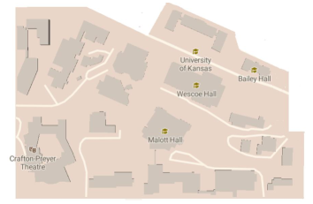
(a) 3D campus of the University of Kansas.

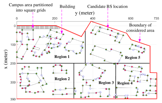
(b) Illustration of campus with different number $B$ of candidate BS locations (i.e., $B\!=\!240$ (blue circles), $B\!=\!184$ (blue circles+red$\ast$), and $B\!=\!130$ (blue circles+red$\ast$+green triangle)) on the building walls and the square grids partitioning the outdoor campus. Five regions with the different active UE densities: the UE density at the $i$th region is $\lambda_{\text{UE},g}^{(i)}\!=\!(2i+2)\times 10^{-4}$, $i=1,2,\ldots,5$.

Figure 3: Campus map of the University of Kansas for outdoor mmWave BS deployment evaluation.

TABLE II: Simulation Parameters

Variables and Description	Values
BS height	$H_{\text{BS}}=10$ m
UE height $H_{\text{UE}}$	$H_{\text{UE}}=1.5$ m
Square grid length $L_{\text{grd}}$	$L_{\text{grd}}=5$ m
Numbers of candidate BS locations	$B=240/184/130$
Numbers of grids	$G=7393$
Parameters for physical blockage in (4)	$\alpha=0.08$, $\beta=0.08$
Number of RF chains $N_{\text{RF}}$	$N_{\text{RF}}=12$
Maximum link distance $R^{\text{max}}$	$R^{\text{max}}=200$ m [43]
Link SINR threshold $z$	$z\!=\!1$
UE access-limited blockage tolerance	$\gamma=0.05$
UE outage tolerance	$\zeta=0.05$
Mainlobe and sidelobe beam gain	$G_{\text{main}}\!=\!15$ dB and $G_{\text{side}}\!=\!-9$ dB [45]
BS transmit power	$P_{\text{Tx}}=1$ Watt [50]
Noise power $\sigma^{2}$	$\sigma^{2}=-104.5$ dBm [51]
Tolerance $\epsilon$ in Algorithm 1	$\epsilon=0.1$

V Simulation Studies

In this section, we numerically evaluate the proposed BS deployment scheme in terms of the deployment cost, computational complexity, and UE outage performance. The geometry in Fig. 3 with dimension $390$ m $\times$ 735 m is considered to evaluate the performance of the proposed BS deployment scheme. Different numbers of candidate BS locations (i.e., $B\!=\!240,B\!=\!184,B=\!130\!$ in Fig. 3(b)) are considered to evaluate the tradeoff between the time complexity in solving the transformed minimum-cost BS selection subproblem (43) and the UE outage performance. Specific parameters of the geometry in Fig. 3 and the considered mmWave systems are summarized in TABLE II. Although different grid $g$ could have different UE density $\lambda_{\text{UE},g}$, we divide the considered geometry into five distinct regions for simplicity as shown in Fig. 3 and assume that the grids in the same region have the same UE density, in which the UE density of the $i$th region is described by $\lambda_{\text{UE}}^{(i)}\!=\!(2i+2)\times 10^{-4}$, $i=1,\ldots,5$. Based on the model in Fig. 3, there are on average $165$ active UEs in the network. Considering the fact that the cost $c_{b}$ in (24a) of installing a BS in an area with higher UE density (e.g., urban area) is, in general, more expensive than that of lower UE density (e.g., rural area), we set the installation cost $c_{b}$ in the $i$th region as $0.2i$, $i=1,\ldots,5$ for simplicity.

V-A Benchmark Schemes

We will compare our proposed BS deployment algorithm against the site-specific mmWave BS deployment strategies below.

• Macro Diversity-Constrained Problem (MDP): The MDP is formed by minimizing the BS deployment cost in (24a) and by requiring each grid to be covered by at least two BSs:

  $$\min\limits_{\mathbf{y}}\!\!\!\!\!\!\!\! \sum_{b=1}^{B}c_{b}y_{b}$$ (44)

  subject to $$\sum_{b=1}^{B}x_{b,g}\geq 2,\;\forall g\in{\mathcal{G}}.$$

  The constraint provides a macro diversity guarantee to each grid, which can be effectively used to manage the physical blockage. The MDP in (44) is ILP. Thus, it can be efficiently solved by using available solvers.

• Average Signal Strength-Guaranteed Problem (ASSGP) in [32]: The underlying idea is to distribute BSs to guarantee a certain level of average received signal strength (RSS). The ASSGP is therefore formed by adding an additional constraint, setting a threshold for the RSS of each UE, to the MDP in (44) below:

  $$\min\limits_{\mathbf{y}}\!\!\!\!\!\!\!\! \sum_{b=1}^{B}c_{b}y_{b}$$ (45)

  subject to $$\sum_{b=1}^{B}x_{b,g}\geq 2,\;\forall g\in{\mathcal{G}}$$

  $$\frac{1}{\sum_{b=1}^{B}x_{b,g}}\sum_{b=1}^{B}x_{b,g}\text{RSS}_{b,g}\geq\text{RSS}_{\text{th}},\forall g\in{\mathcal{G}},$$

  where $\text{RSS}_{b,g}=P_{b,g}+G_{\text{main}}-\text{PL}_{b,g}(r_{b,g})$ in dB is the RSS of the link from BS $b$ to grid $g$ with distance $r_{b,g}$, and the RSS threshold is set to $\text{RSS}_{\text{th}}\!=\!-90$ dB. The problem in (45) is solved by using the heuristic approach proposed in [32].

• Blockage-Guaranteed Greedy Approach (BGGA): In this benchmark, we form a strategy that focuses on providing blockage tolerance. This can be done by replacing the UE outage constraint (24) of our proposed problem in (24) to

  $$\sum_{b\in{\mathcal{B}}}x_{b,g}\mathrm{log}\Big{(}p^{\text{blk}}_{b,g}\!+\!\gamma\left(1-p^{\text{blk}}_{b,g}\right)\Big{)}\!\leq\!\mathrm{log}\left(\zeta\right),\;\forall g\in{\mathcal{G}},$$ (46)

  which is obtained by removing the SINR outage probability in (24). Similar to the proposed algorithm, we decompose the problem into the two separable subproblems. The BS coverage optimization subproblem is first solved by using the algorithm in Section-IV-A. To solve the minimum-cost subset BS selection subproblem with the constraint in (46), we adopt the greedy algorithm (GA) proposed in [34]. In the GA, a new BS is added per iteration that guarantees the constraint (46) for the largest number of grids while minimizing the BS deployment cost. The iteration ends when (46) holds for all $G$ grids.

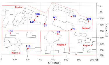
Figure 4: Maximum link distance $r_{b}^{\text{max}}$ in (29) for $10$ candidate BS locations. The $r_{b}^{\text{max}}$ values are best represented by the blue fonts.

V-B Performance Evaluation

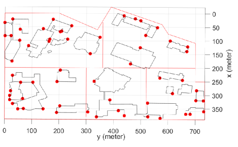
(a) MDP scheme, $61$ deployed BSs with cost $\sum_{b=1}^{B}c_{b}y_{b}=32.8$.

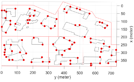
(b) ASSGP scheme, $84$ deployed BSs with cost $\sum_{b=1}^{B}c_{b}y_{b}=45$.

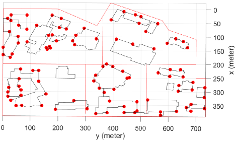
(c) BGGA scheme, $102$ deployed BSs with cost $\sum_{b=1}^{B}c_{b}y_{b}=55$.

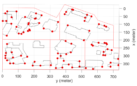
(d) Proposed scheme, $89$ deployed BSs with cost $\sum_{b=1}^{B}c_{b}y_{b}=48.4$.

Figure 5: BS deployment results of the benchmark MDP, ASSGP, BGGA, and proposed scheme under $B\!=\!240$ candidate locations.

In this subsection, we present the BS deployment results obtained by the proposed scheme and the benchmarks MDP, ASSGP, and BGGA. Using these results, we evaluate and compare the link SINR and UE outage for different schemes. We begin with highlighting the result of the Algorithm 1 that yields the maximum link distance for each candidate BS location.

V-B1 BS Coverage Maximization

Fig. 4 presents the maximum link distance $r_{b}^{\text{max}}$ values in (29) at the ten different candidate BS locations, obtained by Algorithm 1. Because the UEs in Region $5$ have the highest density due to the increased UE access-limited blockage, those candidate locations have relatively small coverage radii compared to other regions. In contrast, the candidate BS locations in the open areas of Regions $1$ and $2$ are LoS-visible to many grids but most of the maximum link distances are larger than $100$ meters due to the relatively low UE density. This observation reveals that the maximum link distance depends on both the UE density and the nearby geometry.

V-B2 BS Deployment Cost

Given $B=240$ candidate BS locations shown as blue circles in Fig. 3, the BS deployment results of the proposed method and the benchmark MDP, ASSGP, and BGGA, are displayed in Fig. 5. The numbers of the deployed BSs of the proposed, MDP, ASSGP, and BGGA schemes are given by $89$, $61$, $84$, and $102$, respectively. The proposed scheme and BGGA yield larger numbers of deployed BSs due to the UE access-limited blockage constraint, in which a BS $b$ has a maximum link distance $r_{b}^{\text{max}}\leq R^{\text{max}}$ as in Fig 4 and can only cover a limited number of grids. Among the four strategies, the MDP in Fig. 5(a) deploys the least number of BSs. This happens because the MDP criterion merely focuses on extending the LoS link distance to ensure the macro diversity constraint in (44). In contrast, ASSGA, BGGA, and the proposed scheme attempt to evenly distribute the BSs. This is because the average RSS constraint (45) in ASSGA, the blockage constraint (46) in BGGA, and the UE outage constraint (24) in the proposed scheme control the link distance so that a UE far from its serving BS experiences unsatisfactory link performance. It is not difficult to observe that the BS deployment obtained by the proposed scheme is feasible to the BGGA because the left-hand-side of (46) is a lower bound of that of (24) and the BGGA problem is suboptimally solved by the greedy approach in [34], explaining the inferior performance of BGGA compared to the proposed scheme.

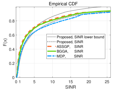
Figure 6: CDF of the links’ SINR and its SINR lower bound $\overline{\text{SINR}}_{b,g}(\mathbf{y}^{\star},\mathbf{X}^{\star})$ in (13).

V-B3 SINR Performance

For each link from BS $b$ to grid $g$ ($x_{b,g}=1$), we collect the $\text{SINR}_{b,g}(\mathbf{y}^{\star},\mathbf{X}^{\star})$ values for $50$ random realizations for the results in Fig.5. The cumulative distribution functions (CDFs) of the collected $\left\{\text{SINR}_{b,g}(\mathbf{y}^{\star},\mathbf{X}^{\star})\right\}$ of the proposed and benchmark schemes are displayed in Fig. 6, where $F(x)$ denotes the CDF of the data that is smaller than or equal to the abscissa $x$. For the proposed scheme, the CDF of the SINR lower bound $\overline{\text{SINR}}_{b,g}(\mathbf{y}^{\star},\mathbf{X}^{\star})$ in (13) is also plotted. It is observed that the MDP reveals the best SINR performance due to the smallest number of deployed BSs and thus lower network interference level. However, this outpacing result is due to the ignorance of the physical and UE access-limited blockages, resulting in the worst UE outage performance as will be shown in Fig. 9. The proposed scheme, deploying $89$ BSs, has a slightly larger number of the deployed BSs than the ASSGP ($84$ BSs), but has better SINR performance since ASSGP does not account for the SINR outdage during its deployment. The BGGA that deploys the largest number of BSs (i.e., $102$ BSs) reveals a worse SINR performance than that of the proposed scheme due to the increased network interference. The SINR outage for a connected link occurs when the SINR is lower than a threshold $z=1$ in TABLE II. It is noticed from Fig. 6 that $77\%$ of the links have $\overline{\text{SINR}}_{b,g}(\mathbf{y}^{\star},\mathbf{X}^{\star})\geq z=1$, while $78\%$ of the links have ${\text{SINR}}_{b,g}(\mathbf{y}^{\star},\mathbf{X}^{\star})\geq z=1$. This reveals that the SINR outage upper bound in (15) (i.e., the SINR lower bound in (13)) is tight for at least $77\%$ links. However, seen from Fig. 6, the gap between the bound and true value grows as the SINR increases.

TABLE III: Proposed BS deployment under different parameter settings.

Different $B$	Parameter setting	Number of BSs	Deployment cost	Running time (minutes)
$B=240$	$N_{RF}\!=\!12$, $\gamma\!=\!0.05,\zeta\!=\!0.05$	89	48.4	45
$B=240$	$N_{RF}\!=\!14$, $\gamma\!=\!0.05,\zeta\!=\!0.05$	88	47.6	77
$B=240$	$N_{RF}\!=\!14$, $\gamma\!=\!0.05,\zeta\!=\!0.1$	82	44.6	78
$B=184$	$N_{RF}\!=\!12$, $\gamma\!=\!0.05,\zeta\!=\!0.05$	Infeasible	Not available	Not available
$B=184$	$N_{RF}\!=\!14$, $\gamma\!=\!0.05,\zeta\!=\!0.05$	Infeasible	Not available	Not available
$B=184$	$N_{RF}\!=\!14$, $\gamma\!=\!0.05,\zeta\!=\!0.1$	84	45.4	51
$B=130$	$N_{RF}\!=\!12$, $\gamma\!=\!0.05,\zeta\!=\!0.05$	Infeasible	Not available	Not available
$B=130$	$N_{RF}\!=\!14$, $\gamma\!=\!0.05,\zeta\!=\!0.1$	Infeasible	Not available	Not available
$B=130$	$N_{RF}\!=\!14$, $\gamma\!=\!0.05,\zeta\!=\!0.2$	50	21.2	19

V-B4 Varying Number of Candidate BS Locations

In TABLE III, we present the results of the proposed BS deployment for different numbers of candidate BS locations as in Fig. 3 and for different sets of parameters. It can be observed that increasing the number of RF chains $N_{\text{RF}}$ decreases the number of deployed BSs. This is because a BS with a larger $N_{\text{RF}}$ can afford a larger $\Phi$ value in (23) and thereby, covers more grids. Moreover, it is noticed that the number of candidate BS locations $B$ also impact to the BS deployment results. When $N_{RF}\!=\!14$, $\gamma\!=\!0.05,\zeta\!=\!0.1$ in TABLE III, two more BSs are deployed when $B=184$ due to the reduced search space for BS deployment compared to the case when $B=240$. However, as we reduce the number of candidate BS locations $B$, it raises the infeasibility issue of the proposed BS deployment scheme as shown in TABLE III.

V-B5 Time Complexity

TABLE III also displays the time complexity of the proposed scheme. The time overhead is measured in minutes using Gurobi [49]. Compared to the time complexities of MDP, ASSGP, BGGA when $B=240,N_{RF}\!=\!12$, $\gamma\!=\!0.05,\zeta\!=\!0.05$, whose running times are $1$ minutes, $5$ minutes, and $12$ minutes, respectively, time complexity of the proposed scheme is exceedingly high. However, considering the fact that our proposed scheme optimally solves the INP in (24) and runs off-line, it is not a serious drawback. As aforementioned, solving the INP in (24) for the large-scale problem size in TABLE II ($B\times G\!=\!1,774,320$) is difficult if not impossible. Directly solving them using available solvers often encounters memory outage or never-ending running time. Although the proposed linearization technique in Lemma 4 introduces twice more additional variables $s_{b,g},\forall b,g$ than the benchmarks, implementing the variable nulling strategy in Section IV-C1 effectively alleviate the computational overhead.

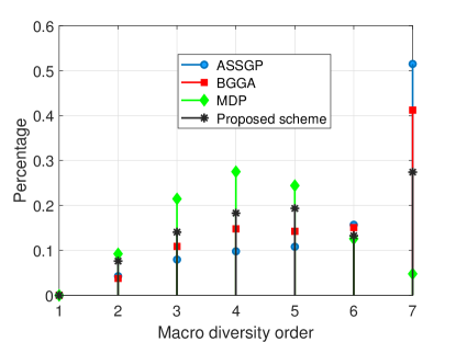
Figure 7: Probabilities of the macro diversity order for the MDP, ASSGP, BGGA, and proposed scheme.

V-B6 Macro Diversity Order Distribution

The macro diversity orders $\sum_{b\in\mathcal{B}}x_{b,g},\!\forall g\!\in\!\mathcal{G}$ in (1) of each scheme are collected and $\Pr\left(\sum_{b}x_{b,g}=i\right)$ are presented in Fig. 7 for the deployment results in Fig. 5. Note that all schemes guarantee a minimum macro diversity order $2$, which is a constraint for the MDP and ASSGP, and an implicit requirement for the BGGA and proposed scheme for UE outage mitigation. Without the UE access-limited blockage constraint, deployed BSs of MDP can cover any LoS-visible grids within $R^{\max}$ and hence it deploys the minimum number of BSs (i.e., $61$ BSs) to produce the largest $\Pr\left(\sum_{b}x_{b,g}=i\right)$ at $i=2,3,4,5$ as seen in Fig. 7. While the proposed scheme has a similar (respectively, smaller) number of deployed BSs to the ASSGP (than the BGGA), its $\Pr\left(\sum_{b}x_{b,g}=i\right)$ at $i=2,3,4,5$ is larger than those of the ASSGP and BGGA, which demonstrates the superior performance of the proposed scheme compared to the benchmarks in terms of providing UE outage guarantees; this will be clear in Fig. 9.

V-B7 UE Access-Limited Blockage Probability

In Fig. 8, given the BS deployment results in Fig. 5, we collect the UE access-limited blockage probabilities for each BS and demonstrate the CDFs of $\left\{\rho_{b,g}({\mathbf{x}}_{b})\;\text{in}\;\eqref{express2}\;\;\forall b\in{\mathcal{B}}\;\text{with}\;y_{b}\!=\!1\right\}$. It can be observed from the curves that the proposed scheme and BGGA deploy the BSs to guarantee that each UE’s access-limited blockage probability is limited by the tolerance $\gamma\!=\!0.05$ in TABLE II. However, around $30\sim 40\%$ of the deployed BSs with the MDP and ASSGP schemes have the UE access-limited blockage probability larger than $0.05$. It should be emphasized that this stark guarantee is achieved by deploying $89$ BSs of the proposed scheme, while the MDP, ASSGP, and BGGA deploy $61$, $84$, and $102$ BSs, respectively.

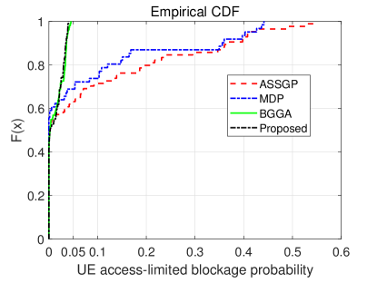
Figure 8: CDF of the collected UE access-limited blockage statistics, i.e., CDFs of $\left\{\rho_{b,g}({\mathbf{x}}_{b})\;\text{in}\;\eqref{express2}\;\;\forall b\in{\mathcal{B}}\;\text{with}\;y_{b}\!=\!1\right\}$.

V-B8 UE Outage Probability

Based on the BS deployment results in Fig. 5, we collect the UE outage probabilities in (24). The CDFs of the collected UE outage probabilities are demonstrated in Fig. 9. It is evident that the proposed scheme guarantees the UE outage probability with the specified tolerance $\zeta\!=\!0.05$ in TABLE II. Even through the ASSGP deploys the similar number of BSs as the proposed scheme, its UE outage performance is much worse than the proposed scheme and nearly $12\%$ UEs have outage probability larger than $0.1$. The BGGA exhibits the similar UE outage statistics to the proposed scheme. However, it fails to provides the guarantee and its performance is achieved by deploying $13$-more BSs than the proposed scheme.

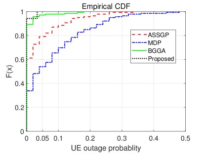
Figure 9: CDF of the collected UE outage probabilities.

VI Conclusions

We addressed important mmWave connectivity challenges in a 3D urban geometry by proposing a link quality-guaranteed minimum-cost mmWave BS deployment scheme that jointly optimizes the BS placement and cell coverage. To mathematically formulate the problem, we first introduced the stochastic mmWave link state model and used it to characterize the BS association and UE outage constraints. The BS deployment problem was then formulated as INP, which was optimally solved by decomposing it into two separable subproblems: (i) BS coverage optimization problem and (ii) minimum subset BS selection problem. We provided the optimal solutions for these subproblems as well as their theoretical justifications. Simulation results demonstrated the efficacy of the proposed scheme in terms of the BS deployment cost, computational complexity, UE access-limited blockage, and UE outage performance. Compared to the MDP, ASSGP, and BGGA benchmarks, our proposed algorithm provides guaranteed tolerance to UE access-limited blockage and UE outage. It should be noted here that our main goal in this work was to study the principle of minimum-cost BS deployment for combined coverage and link quality constraints in mmWave networks, and through simulations describe the gain that can be expected by taking on such an approach. One major drawback of the proposed scheme was that the time complexity is exceedingly high compared to other benchmarks. However, considering the fact that the BS deployment planning is done off-line in practice, our proposed scheme optimally solves the INP in (24), and the proposed scheme provided stark outage guarantees, the high time complexity is not a serious drawback.

References

- [1] S. Hur, T. Kim, D. J. Love, J. V. Krogmeier, T. A. Thomas, and A. Ghosh, “Millimeter wave beamforming for wireless backhaul and access in small cell networks,” IEEE Transactions on Communications, vol. 61, no. 10, pp. 4391–4403, Oct. 2013.
- [2] B. P. S. Sahoo, C. Chou, C. Weng, and H. Wei, “Enabling millimeter-wave 5g networks for massive IoT applications: A closer look at the issues impacting millimeter-waves in consumer devices under the 5G framework,” IEEE Consumer Electronics Magazine, vol. 8, no. 1, pp. 49–54, Jan 2019.
- [3] V. Raghavan, A. Partyka, A. Sampath, S. Subramanian, O. H. Koymen, K. Ravid, J. Cezanne, K. Mukkavilli, and J. Li, “Millimeter-wave MIMO prototype: Measurements and experimental results,” IEEE Communications Magazine, vol. 56, no. 1, pp. 202–209, Jan 2018.
- [4] R. W. Heath, N. González-Prelcic, S. Rangan, W. Roh, and A. M. Sayeed, “An overview of signal processing techniques for millimeter wave MIMO systems,” IEEE Journal of Selected Topics in Signal Processing, vol. 10, no. 3, pp. 436–453, 2016.
- [5] H. Ghauch, T. Kim, M. Bengtsson, and M. Skoglund, “Subspace estimation and decomposition for large millimeter-wave mimo systems,” IEEE Journal of Selected Topics in Signal Processing, vol. 10, no. 3, pp. 528–542, April 2016.
- [6] A. Alkhateeb, R. W. Heath, and G. Leus, “Achievable rates of multi-user millimeter wave systems with hybrid precoding,” in 2015 IEEE International Conference on Communication Workshop (ICCW), Jun. 2015, pp. 1232–1237.
- [7] W. Zhang, T. Kim, D. J. Love, and E. Perrins, “Leveraging the restricted isometry property: Improved low-rank subspace decomposition for hybrid millimeter-wave systems,” IEEE Transactions on Communications, vol. 66, no. 11, pp. 5814–5827, Nov 2018.
- [8] O. E. Ayach, S. Rajagopal, S. Abu-Surra, Z. Pi, and R. W. Heath, “Spatially sparse precoding in millimeter wave MIMO systems,” IEEE Transactions on Wireless Communications, vol. 13, no. 3, pp. 1499–1513, Mar. 2014.
- [9] A. Alkhateeb, O. E. Ayach, G. Leus, and R. W. Heath, “Channel estimation and hybrid precoding for millimeter wave cellular systems,” IEEE Journal of Selected Topics in Signal Processing, vol. 8, no. 5, pp. 831–846, Oct. 2014.
- [10] T. S. Rappaport, Y. Xing, G. R. MacCartney, A. F. Molisch, E. Mellios, and J. Zhang, “Overview of millimeter wave communications for fifth-generation (5G) wireless networks—with a focus on propagation models,” IEEE Transactions on Antennas and Propagation, vol. 65, no. 12, pp. 6213–6230, 2017.
- [11] T. Bai, R. Vaze, and R. W. Heath, “Analysis of blockage effects on urban cellular networks,” IEEE Transactions on Wireless Communications, vol. 13, no. 9, pp. 5070–5083, Sep. 2014.
- [12] M. Dong and T. Kim, “Interference analysis for millimeter-wave networks with geometry-dependent first-order reflections,” IEEE Transactions on Vehicular Technology, vol. 67, no. 12, pp. 12 404–12 409, Dec. 2018.
- [13] J. Choi, “On the macro diversity with multiple BSs to mitigate blockage in millimeter-wave communications,” IEEE Communications Letters, vol. 18, no. 9, pp. 1653–1656, Sep. 2014.
- [14] A. Alizadeh and M. Vu, “Time-fractional user association in millimeter wave MIMO networks,” in 2018 IEEE International Conference on Communications (ICC), May 2018, pp. 1–6.
- [15] H. Zhang, S. Huang, C. Jiang, K. Long, V. C. M. Leung, and H. V. Poor, “Energy efficient user association and power allocation in millimeter-wave-based ultra dense networks with energy harvesting base stations,” IEEE Journal on Selected Areas in Communications, vol. 35, no. 9, pp. 1936–1947, Sep. 2017.
- [16] (2019, Oct) Precision planning for 5G era network with smallcells, white paper. [Online]. Available: https://www.scf.io/en/documents/230_Precision_planning_for_5G_Era_networks_with_small_cells.php
- [17] J. Peng, P. Hong, and K. Xue, “Energy-aware cellular deployment strategy under coverage performance constraints,” IEEE Transactions on Wireless Communications, vol. 14, no. 1, pp. 69–80, Jan. 2015.
- [18] G. Zhao, S. Chen, L. Zhao, and L. Hanzo, “Joint energy-spectral-efficiency optimization of CoMP and BS deployment in dense large-scale cellular networks,” IEEE Transactions on Wireless Communications, vol. 16, no. 7, pp. 4832–4847, Jul. 2017.
- [19] B. Yang, G. Mao, X. Ge, M. Ding, and X. Yang, “On the energy-efficient deployment for ultra-dense heterogeneous networks with NLoS and LoS transmissions,” IEEE Transactions on Green Communications and Networking, vol. 2, no. 2, pp. 369–384, Jun. 2018.
- [20] P. Mekikis, E. Kartsakli, A. Antonopoulos, A. S. Lalos, L. Alonso, and C. Verikoukis, “Two-tier cellular random network planning for minimum deployment cost,” in IEEE International Conference on Communications, Jun. 2014, pp. 1248–1253.
- [21] C. Peng, L. Wang, and C. Liu, “Optimal base station deployment for small cell networks with energy-efficient power control,” in 2015 IEEE International Conference on Communications (ICC), Jun. 2015, pp. 1863–1868.
- [22] M. Dong, T. Kim, J. Wu, and E. W. M. Wong, “Cost-efficient millimeter wave base station deployment in manhattan-type geometry,” IEEE Access, vol. 7, pp. 149 959–149 970, 2019.
- [23] S. Chatterjee, M. J. Abdel-Rahman, and A. B. MacKenzie, “Optimal base station deployment with downlink rate coverage probability constraint,” IEEE Wireless Communications Letters, vol. 7, no. 3, pp. 340–343, Jun. 2018.
- [24] C. Fan, T. Zhang, and Z. Zeng, “Energy-efficient base station deployment in HetNet based on traffic load distribution,” in 2017 IEEE 85th Vehicular Technology Conference (VTC Spring), Jun. 2017, pp. 1–5.
- [25] M. A. Yigitel, O. D. Incel, and C. Ersoy, “Dynamic BS topology management for green next generation HetNets: An urban case study,” IEEE Journal on Selected Areas in Communications, vol. 34, no. 12, pp. 3482–3498, Dec. 2016.
- [26] C. C. Coskun and E. Ayanoglu, “Energy-efficient base station deployment in heterogeneous networks,” IEEE Wireless Communications Letters, vol. 3, no. 6, pp. 593–596, Dec. 2014.
- [27] Y. Lu, H.-W. Hsu, and L.-C. Wang, “Performance model and deployment strategy for mm-wave multi-cellular systems,” in 2016 25th Wireless and Optical Communication Conference, May 2016, pp. 1–4.
- [28] S. S. Szyszkowicz, A. Lou, and H. Yanikomeroglu, “Automated placement of individual millimeter-wave wall-mounted base stations for line-of-sight coverage of outdoor urban areas,” IEEE Wireless Communications Letters, vol. 5, no. 3, pp. 316–319, Jun. 2016.
- [29] N. Palizban, S. Szyszkowicz, and H. Yanikomeroglu, “Automation of millimeter wave network planning for outdoor coverage in dense urban areas using wall-mounted base stations,” IEEE Wireless Communications Letters, vol. 6, no. 2, pp. 206–209, Apr. 2017.
- [30] M. Gonzalez and J. Thompson, “An energy efficient base station deployment for mm-wave based wireless backhaul,” in 2016 IEEE 27th Annual International Symposium on Personal, Indoor, and Mobile Radio Communications (PIMRC), Sep. 2016, pp. 1–6.
- [31] Y. Zhang, L. Dai, and E. W. M. Wong, “Optimal BS deployment and user association for 5G millimeter wave communication networks,” IEEE Transactions on Wireless Communications, vol. 20, no. 5, pp. 2776–2791, 2021.
- [32] I. Mavromatis, A. Tassi, R. J. Piechocki, and A. R. Nix, “Efficient millimeter-wave infrastructure placement for city-scale ITS,” CoRR, vol. abs/1903.01372, 2019. [Online]. Available: http://arxiv.org/abs/1903.01372
- [33] M. Dong, T. Kim, J. Wu, and W. M. E. Wong, “Millimeter-wave base station deployment using the scenario sampling approach,” IEEE Transactions on Vehicular Technology, vol. 69, no. 11, pp. 14 013–14 018, 2020.
- [34] M. Naderi Soorki, W. Saad, and M. Bennis, “Optimized deployment of millimeter wave networks for in-venue regions with stochastic users’ orientation,” IEEE Transactions on Wireless Communications, vol. 18, no. 11, pp. 5037–5049, 2019.
- [35] K. Shen, Y. Liu, D. Y. Ding, and W. Yu, “Flexible multiple base station association and activation for downlink heterogeneous networks,” IEEE Signal Processing Letters, vol. 24, no. 10, pp. 1498–1502, Oct. 2017.
- [36] M. Feng, S. Mao, and T. Jiang, “BOOST: Base station on-off switching strategy for green massive MIMO hetnets,” IEEE Transactions on Wireless Communications, vol. 16, no. 11, pp. 7319–7332, Nov. 2017.
- [37] X. Lin and S. Wang, “Joint user association and base station switching on/off for green heterogeneous cellular networks,” in 2017 IEEE International Conference on Communications (ICC), May 2017, pp. 1–6.
- [38] J. Kim, W. S. Jeon, and D. G. Jeong, “Base-station sleep management in open-access femtocell networks,” IEEE Transactions on Vehicular Technology, vol. 65, no. 5, pp. 3786–3791, May 2016.
- [39] J. Vales-Alonso, F. Parrado-García, P. López-Matencio, J. Alcaraz, and F. González-Castaño, “On the optimal random deployment of wireless sensor networks in non-homogeneous scenarios,” Ad Hoc Networks, vol. 11, no. 3, pp. 846–860, 2013.
- [40] M. Haenggi, “Stochastic geometry for wireless networks,” Cambridge, U.K.: Cambridge Univ. Press, 2012.
- [41] M. Dong, W. Chan, T. Kim, K. Liu, H. Huang, and G. Wang, “Simulation study on millimeter wave 3D beamforming systems in urban outdoor multi-cell scenarios using 3D ray tracing,” in IEEE 26th Annual International Symposium on PIMRC, Aug. 2015, pp. 2265–2270.
- [42] G. T. 38.211. (2020, Jan.) Physical channels and modulation. [Online]. Available: https://portal.3gpp.org/desktopmodules/Specifications/SpecificationDetails.aspx?specificationId=3213
- [43] T. S. Rappaport, S. Sun, R. Mayzus, H. Zhao, Y. Azar, K. Wang, G. N. Wong, J. K. Schulz, M. Samimi, and F. Gutierrez, “Millimeter wave mobile communications for 5G cellular: It will work!” IEEE Access, vol. 1, pp. 335–349, May 2013.
- [44] T. Bai and R. W. Heath, “Coverage and rate analysis for millimeter-wave cellular networks,” IEEE Transactions on Wireless Communications, vol. 14, no. 2, pp. 1100–1114, Feb. 2015.
- [45] M. D. Renzo, “Stochastic geometry modeling and analysis of multi-tier millimeter wave cellular networks,” IEEE Transactions on Wireless Communications, vol. 14, no. 9, pp. 5038–5057, Sep. 2015.
- [46] ——, “Stochastic geometry modeling and analysis of multi-tier millimeter wave cellular networks,” IEEE Transactions on Wireless Communications, vol. 14, no. 9, pp. 5038–5057, Sep. 2015.
- [47] R. L. Strei, Poisson Point Processess: Imaging, Tracking, and Sensing. Springer US, Sep. 2010.
- [48] D. Li and X. Sun, Nonlinear Integer Programming. Springer US, 2006.
- [49] Gurobi. (2018) Gurobi optimier quick start guide. [Online]. Available: https://www.gurobi.com/wp-content/plugins/hd_documentations/content/pdf/quickstart_windows_8.1.pdf
- [50] G. R. MacCartney and T. S. Rappaport, “Millimeter-wave base station diversity for 5g coordinated multipoint (CoMP) applications,” IEEE Transactions on Wireless Communications, vol. 18, no. 7, pp. 3395–3410, 2019.
- [51] L. Encyclopedia. (2021) LTE radio link budgeting and RF planning. [Online]. Available: https://sites.google.com/site/lteencyclopedia/lte-radio-link-budgeting-and-rf-planning