Q-error Bounds of Random Uniform Sampling for Cardinality Estimation

Abstract

Random uniform sampling has been studied in various statistical tasks but few of them have covered the Q-error metric for cardinality estimation (CE). In this paper, we analyze the confidence intervals of random uniform sampling with and without replacement for single-table CE. Results indicate that the upper Q-error bound depends on the sample size and true cardinality. Our bound gives a rule-of-thumb for how large a sample should be kept for single-table CE.

1 Introduction

Cardinality estimation (CE) is the key to various tasks such as query optimization and approximate query processing. Production systems apply histograms [15] and sketches such as Count-Min and HyperLogLog [5] for fast and accurate estimates [2, 4, 3, 5, 10, 6, 18]. Random uniform sampling has been studied in this context for a long period of time; despite various prior analyses for random sampling [12, 11], few have covered the Q-error metric for CE.

In this paper, we analyze the Q-error bounds for sampling-based single-table CE with and without replacement. Based on existing statistical tools such as the Chernoff Bound and the Bernstein-Serfling’s Inequality, our analyses show the confidence intervals for the Q-error are less than a threshold given the sample size and true cardinality. The upper Q-error bound for random sampling with replacement is agnostic to the size of the original table. Our analyses can be used as a rule-of-thumb for how large a sample should be kept to reach a specific Q-error at a given confidence interval, as well as a simple accuracy baseline for other CE solutions [17].

In the following paper, Section 2 defines the problem setup. Section 3 and Section 4 analyze the upper error bounds of random sampling with and without replacement for single-table CE. We discuss link to related work in Section 5.

2 Problem Setup

Let $t$ be a table with $n$ rows and $m$ columns, and $\hat{t}$ be a sample of $k$ rows drawn uniformly at random from $t$. Suppose $pn$ rows from $t$ satisfy the predicate, where $p\in[0,1]$ represents the probability (aka selectivity) that a row in the table satisfies the given predicate. Cardinality estimation (CE), i.e., estimating $np$ given a predicate, can be formulated as an application of Binomial distribution (Sum of Independent Bernoulli Trials), in which each random variable (corresponding to each row) takes the value of 1/0 for satisfying the predicate or not.

Let $X=pn=\sum\limits_{i=0}^{n}x_{i}$ be the cardinality of the predicate in the original table, where $x_{i}=1$ if row $i$ satisfies the predicate. Let $\hat{X}=\sum\limits_{i=0}^{k}\hat{x}_{i}$ be the cardinality of the predicate on the sampled table. We use $\mu=\mathds{E}[\hat{X}]=kp$ as the expected number of rows that satisfy the predicate in the sampled table. The population variance is defined as $\sigma^{2}=\frac{1}{n}\sum\limits_{i=0}^{n}(x_{i}-p)^{2}=\mathds{E}[x_{i}^{2}]-\mathds{E}[x_{i}]^{2}=(1^{2}\times p+0^{2}\times(1-p))-p^{2}=p(1-p)$.

Following recent CE work [8, 21, 13, 16], we use the Q-error metric in our analysis for evaluating the estimation accuracy:

$${\tt Q\mbox{-}error}=\max(\frac{\texttt{true}}{\texttt{est}},\frac{\texttt{est}}{\texttt{true}}),$$

where est is the estimated cardinality and true is the true cardinality. In practice, we replace $\texttt{est}=\max(\texttt{est},1)$ and $\texttt{true}=\max(\texttt{true},1)$ to avoid divide-by-zero. Q-error=1 indicates a perfect prediction.

3 Bounds of Sampling with Replacement

Random uniform sampling with replacement under the independent and identically distributed (i.i.d.) assumption is widely applied in modern machine learning (e.g., bootstrap [9]). Applying Chernoff Bound to sampling with replacement gives us a concise bound with the Q-error metric. We also incorporate error bounds from Bernstein’s Inequality to tighten the bound.

For cardinality estimation over single tables, the Q-error of random uniform sampling with replacement is bounded by

$$\mathds{P}(\text{Q-error $\leq$ q})\geq 1-\Omega-\Psi,where$$

$$\Omega =\min\Bigg{(}\Big{(}\cfrac{e^{q-1}}{q^{q}}\Big{)}^{pk},\exp\Big{(}-\frac{k(pq-p)^{2}}{2\sigma^{2}+2(pq-p)/3}\Big{)}\Bigg{)},$$

$$\Psi =\min\Bigg{(}\Big{(}e^{(\frac{1}{q}-1)}q^{\frac{1}{q}}\Big{)}^{pk},\exp\Big{(}-\frac{k(p-p/q)^{2}}{2\sigma^{2}+2(p-p/q)/3}\Big{)}\Bigg{)}.$$

In the case when the probability $\mathds{P}(\text{Q-error $\leq$ q})$ is negative (i.e. $\Omega+\Psi>1$), we replace it with zero. $\Omega$ is the probability for over-estimation and $\Psi$ is the probability for under-estimation. We further show the result with Hoeffding’s inequality in Appendix, since adding it can only tighten the bounds slightly in some corner cases.

From Theorem 3, we can see that the final error $q$ is agnostic to the number of rows $n$ of the original table. The bound is only relevant to the number of samples $k$ and the true cardinality $p$. We give the detailed analyses below.

CE bounded by Chernoff. The Chernoff bound [Reference 20, Corollary 4.2] for the sum of Bernoulli trials can be stated as the following inequalities, where $\delta\in[0,1]$:

$$\mathds{P}(\hat{X}\geq(1+\delta)\mu)\leq\Big{(}\cfrac{e^{\delta}}{(1+\delta)^{(1+\delta)}}\Big{)}^{\mu},$$ (1)

$$\mathds{P}(\hat{X}\leq(1-\delta)\mu)\leq\Big{(}\cfrac{e^{-\delta}}{(1-\delta)^{(1-\delta)}}\Big{)}^{\mu},$$ (2)

Let $q\geq 1$ be the q-error, and we have the over-estimation probability

$$\mathds{P}(Pred\geq qX) =\mathds{P}(\hat{X}\geq q\mu)$$

(Let $$(1+\delta)=q$$ and apply (1))

$$\leq\Big{(}\cfrac{e^{\delta}}{(1+\delta)^{(1+\delta)}}\Big{)}^{\mu}$$

$$=\Big{(}\cfrac{e^{q-1}}{q^{q}}\Big{)}^{pk}=\Omega.$$

Similarly, we have the under-estimation probability

$$\mathds{P}(Pred\leq\frac{1}{q}X) =\mathds{P}(\hat{X}\leq\frac{1}{q}\mu)$$

(Let $$(1-\delta)=\frac{1}{q}$$ and apply (2))

$$\leq\Big{(}\cfrac{e^{-\delta}}{(1-\delta)^{(1-\delta)}}\Big{)}^{\mu}$$

$$=\Big{(}e^{(\frac{1}{q}-1)}q^{\frac{1}{q}}\Big{)}^{pk}=\Psi.$$

Bound 1

By applying the Chernoff Bound, Q-error from random uniform sampling with replacement is bounded by:

$$\mathds{P}(\text{Q-error $\leq$ q}) \geq\mathds{P}(\text{Q-error $<$ q})$$

$$=1-\mathds{P}(\text{Q-error $\geq$ q})$$

$$=1-\mathds{P}(Pred\geq qX)-\mathds{P}(Pred\leq\frac{1}{q}X)$$

$$=1-\Omega-\Psi$$

$$\geq 1-\Big{(}\cfrac{e^{q-1}}{q^{q}}\Big{)}^{pk}-\Big{(}e^{(\frac{1}{q}-1)}q^{\frac{1}{q}}\Big{)}^{pk}.$$

CE bounded by the Bernstein Inequality. The Bernstein inequality [Reference 1, Proposition 1.4] can be written as,

$$\mathds{P}\Bigg{(}\cfrac{\sum\limits_{t=1}^{k}(x_{t}-\mu_{x})}{k}>\epsilon\Bigg{)}\leq\exp\Big{(}-\cfrac{k\epsilon^{2}}{2\sigma^{2}+2M\epsilon/3}\Big{)},$$ (3)

where $M=\max\limits_{i=0}^{n}|x_{i}|$ and $\epsilon>0$. In our Bernoulli case, $M=1$, and $\mu_{x}=p$ is the population mean. Therefore, we have

$$\mathds{P}(Pred>qX) =\mathds{P}(\hat{X}>kpq)$$

$$=\mathds{P}(\hat{X}-kp>kpq-kp)$$

$$=\mathds{P}\Bigg{(}\frac{\sum\limits_{t=1}^{k}(X_{t}-p)}{k}>pq-p\Bigg{)}$$

(Let $$\epsilon=pq-p$$)

$$=\mathds{P}\Bigg{(}\frac{\sum\limits_{t=1}^{k}(X_{t}-p)}{k}>\epsilon\Bigg{)}$$

$$\leq\exp\Big{(}-\cfrac{k\epsilon^{2}}{2\sigma^{2}+2M\epsilon/3}\Big{)}=\exp\Big{(}-\frac{k(pq-p)^{2}}{2\sigma^{2}+2(pq-p)/3}\Big{)}=\Omega,$$

$$\mathds{P}(Pred<X/q) =\mathds{P}(\hat{X}<\frac{kp}{q})$$

$$=\mathds{P}(k-\hat{Y}<\frac{kp}{q})$$

$$=\mathds{P}(\hat{Y}>k-\frac{kp}{q})$$

$$=\mathds{P}(\hat{Y}-k\bar{p}>k-\frac{kp}{q}-k\bar{p})$$

$$=\mathds{P}\Bigg{(}\frac{\sum\limits_{t=1}^{k}(Y_{t}-\bar{p})}{k}>1-p/q-(1-p)\Bigg{)}$$

$$=\mathds{P}\Bigg{(}\frac{\sum\limits_{t=1}^{k}(Y_{t}-\bar{p})}{k}>p-p/q\Bigg{)}$$

(Let $$\epsilon=p-p/q$$)

$$=\mathds{P}\Bigg{(}\frac{\sum\limits_{t=1}^{k}(Y_{t}-\bar{p})}{k}>\epsilon\Bigg{)}$$

$$\leq\exp\Big{(}-\cfrac{k\epsilon^{2}}{2\sigma^{2}+2M\epsilon/3}\Big{)}=\exp\Big{(}-\frac{k(p-p/q)^{2}}{2\sigma^{2}+2(p-p/q)/3}\Big{)}=\Psi.$$

Bound 2

By applying the Bernstein’s Inequality, the Q-error from random uniform sampling with replacement is bounded by:

$\mathds{P}(\text{Q-error $\leq$ q})\geq 1-\Omega-\Psi=1-\exp\Big{(}-\frac{k(pq-p)^{2}}{2\sigma^{2}+2(pq-p)/3}\Big{)}-\exp\Big{(}-\frac{k(p-p/q)^{2}}{2\sigma^{2}+2(p-p/q)/3}\Big{)}$.

Putting together the $\Omega$ and $\Psi$ in the above bounds, we can derive Theorem 3.

Visualization. Figure 1 plots and compares the bounds shown in this section. With only 100 samples (rows), Bound 1 and 2 already demonstrate some tightness: the Q-error is likely to be small (more than 80% chance with $q\leq 2$) when a query predicate has a cardinality of $p=0.2$; with 1K samples, the Q-error is almost always small ($q\leq$2). Figures 2 and 3 further demonstrate the probability with different $p$ values and the Q-error with 95% confidence.

We also show in Figure 4 the 3-D plotting of the probability that random sampling has a Q-error that is better than a given threshold. At a small sample size such as 100 or 1K rows irrelevant to the table size, random uniform sampling with replacement already provides a promising q-error and has a tight bound.

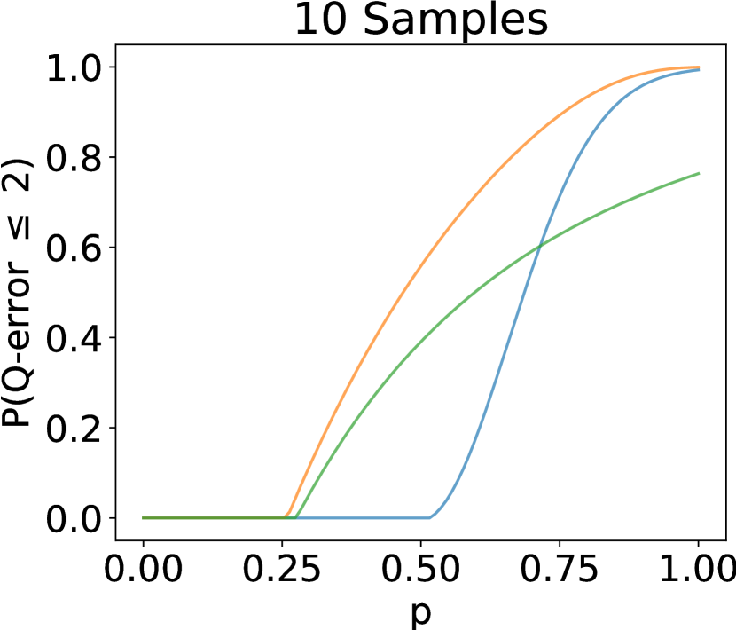
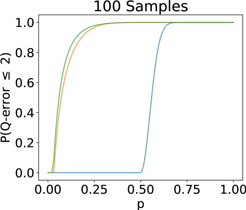
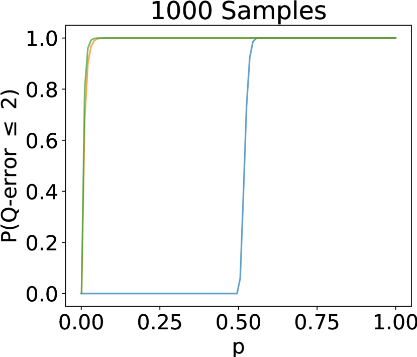
Figure 1: Plotting and comparing the Chernoff, Bernstein’s Inequality and Hoeffding’s Inequality bounds (see Appendix).

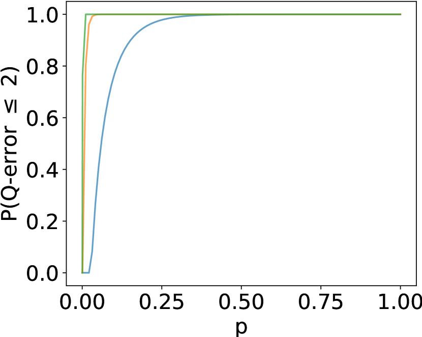
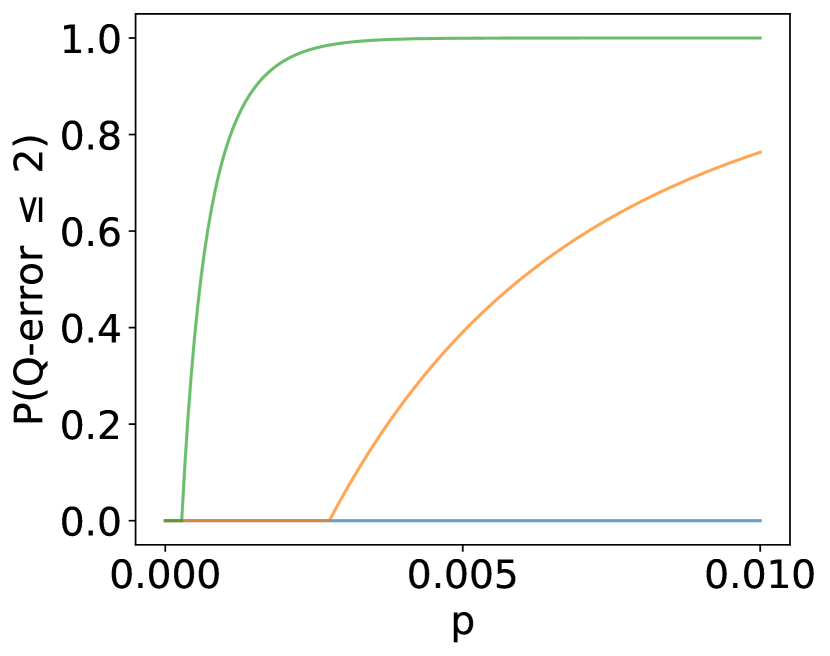
Figure 2: Plotting the bounds in terms of $p$. (Left) Results for $p\in(0,100\%]$. (Right) Results for $p\in(0,1\%]$.

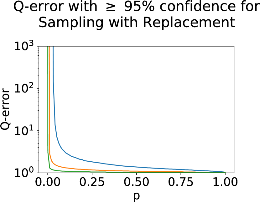
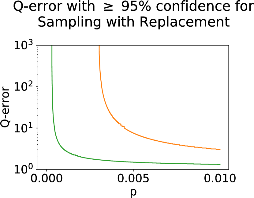
Figure 3: Plotting the Q-error with 95% confidence in terms of $p$. (Left) Results for $p\in(0,100\%]$. (Right) Results for $p\in(0,1\%]$.

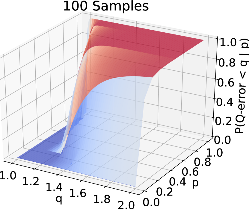
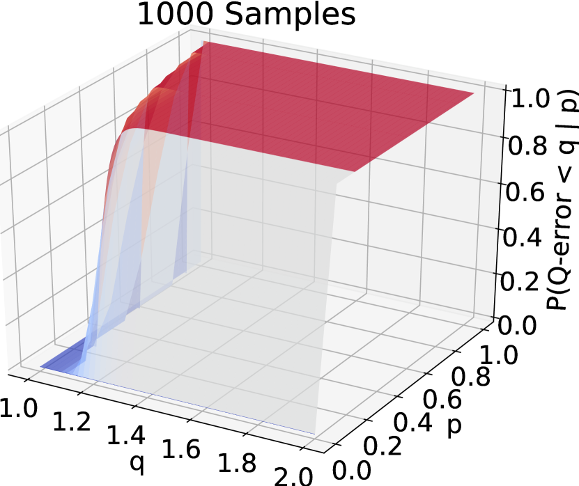
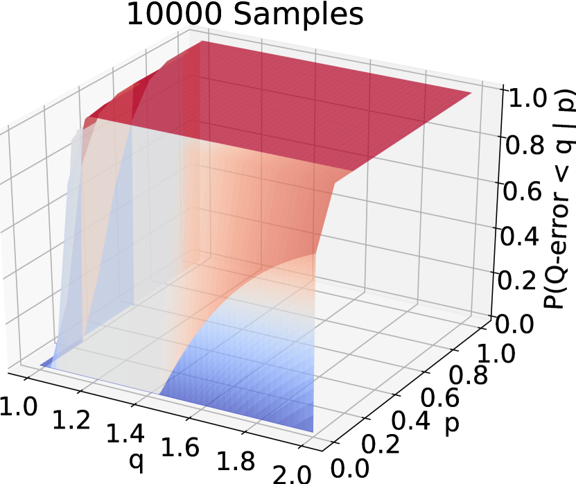
Figure 4: 3D plotting of the probability that random uniform sampling’s error (z-axis) is better than $q$ with a predicate cardinality $p$.

4 Bounds of Sampling without Replacement

When samples are drawn uniformly at random without replacement, we assume there are at least 2 rows. The Hoeffding-Serfling inequality and the Bernstein-Serfling inequality developed in a recent study [1] founded Theorem 4 for random uniform sampling without replacement. Adding Serfling’s results further gives a tighter bound.

For cardinality estimation over single tables, the Q-error of random uniform sampling without replacement is bounded by

$$\mathds{P}(\text{Q-error}\leq q)\geq 1-\Omega-\Psi\text{, where}$$

$$\Omega =\min\Bigg{(}2\exp\Big{(}-\frac{k}{\zeta^{2}}(-\sqrt{2\zeta\rho\sigma^{2}(pq-p)+\rho^{2}\sigma^{4}}+(pq-p)\zeta+\sigma^{2}\rho)\Big{)},$$

$$~{}~{}~{}~{}~{}~{}~{}~{}~{}~{}~{}~{}~{}~{}\exp\Big{(}-\cfrac{2k(pq-p)^{2}}{\rho}\Big{)}\Bigg{)},$$

$$\Psi =\min\Bigg{(}2\exp\Big{(}-\frac{k}{\zeta^{2}}(-\sqrt{2\zeta\rho\sigma^{2}(p-p/q)+\rho^{2}\sigma^{4}}+(p-p/q)\zeta+\sigma^{2}\rho)\Big{)},$$

$$~{}~{}~{}~{}~{}~{}~{}~{}~{}~{}~{}~{}~{}~{}\exp\Big{(}-\cfrac{2k(p-p/q)^{2}}{\rho}\Big{)}\Bigg{)}.$$

CE bounded by Hoeffding-Serfling. For convenience, we define

$\rho=\begin{cases}1-(k-1)/n&\text{if $k\leq n/2$}\\ (1-k/n)(1+1/k)&\text{if $k>n/2$}\end{cases}$ , and $\zeta=\begin{cases}4/3+\sqrt{\frac{k(k-1)}{n(n-k+1)}}&\text{if $k\leq n/2$}\\ 4/3+\sqrt{\frac{(n-k-1)(n-k)}{(k+1)n}}&\text{if $k>n/2$}.\end{cases}$

Let $\chi=(r_{1},...,r_{n})$ be a finite population of $n$ rows. We sample $k$ rows (i.e. $x_{1},...,x_{k}$) without replacement from the population such that $k<n$. Denote $\mathds{E}[r_{i}]=\mu_{x}$, $a=\min\limits_{1\leq i\leq n}r_{i}$, and $b=\max\limits_{1\leq i\leq n}r_{i}$. The Hoeffding-Serfling inequality [Reference 1, Corollary 2.5] can be written as:

$\mathds{P}\Bigg{(}\cfrac{\sum\limits_{t=1}^{k}(x_{t}-\mu_{x})}{k}>(b-a)\sqrt{\cfrac{\rho\log(1/\delta)}{2k}}\Bigg{)}\leq\delta$,

where $\delta\in[0,1]$. For Bernoulli distribution, we can simplify these two inequalities by $a=0$, $b=1$, and $\sigma^{2}=p(1-p)$.

Let $\delta=\exp\Big{(}-\frac{2k(pq-p)^{2}}{\rho}\Big{)}$. Denote $Y_{i}=\neg X_{i}$ such that $Y_{i}=0$ if the sampled row satisfy the predicate and $y_{i}=1$ if the row does not satisfy the predicate. We have $\hat{Y}=\sum\limits_{i=0}^{k}\hat{y}_{i}$ on the sample. It is easy to see $\hat{X}=k-\hat{Y}$. We denote $\bar{p}=\mathds{E}[Y_{i}]=1-p$. The variances for $Y$ is $\bar{p}(1-\bar{p})=(1-p)p$. By applying the Hoeffding-Serfling inequality, we have the over-estimation probability as

$$\mathds{P}(Pred>qX) =\mathds{P}(\hat{X}>kpq)$$

$$=\mathds{P}(\hat{X}-kp>kpq-kp)$$

$$=\mathds{P}\Bigg{(}\frac{\sum\limits_{t=1}^{k}(X_{t}-p)}{k}>pq-p\Bigg{)}$$

$$=\mathds{P}\Bigg{(}\frac{\sum\limits_{t=1}^{k}(X_{t}-p)}{k}>\sqrt{\cfrac{\rho\log(1/\delta)}{2k}}\Bigg{)}$$

$$\leq\delta=\exp\Big{(}-\frac{2k(pq-p)^{2}}{\rho}\Big{)}=\Omega.$$

Let $\delta=\exp\Big{(}-\frac{2k(p-p/q)^{2}}{\rho}\Big{)}$. We have the under-estimation probability as

$$\mathds{P}(Pred<X/q) =\mathds{P}(\hat{X}<\frac{kp}{q})$$

$$=\mathds{P}(k-\hat{Y}<\frac{kp}{q})$$

$$=\mathds{P}(\hat{Y}>k-\frac{kp}{q})$$

$$=\mathds{P}(\hat{Y}-k\bar{p}>k-\frac{kp}{q}-k\bar{p})$$

$$=\mathds{P}\Bigg{(}\frac{\sum\limits_{t=1}^{k}(Y_{t}-\bar{p})}{k}>1-p/q-(1-p)\Bigg{)}$$

$$=\mathds{P}\Bigg{(}\frac{\sum\limits_{t=1}^{k}(Y_{t}-\bar{p})}{k}>p-p/q\Bigg{)}$$

$$\leq\delta=\exp\Big{(}-\frac{2k(p-p/q)^{2}}{\rho}\Big{)}=\Psi.$$

Bound 3

By applying the Hoeffding-Serfling Inequality, the Q-error of random uniform sampling without replacement is bounded by

$$\mathds{P}(\text{Q-error $\leq$ q}) \geq 1-\Omega-\Psi=1-\exp\Big{(}-\cfrac{2k(pq-p)^{2}}{\rho}\Big{)}-\exp\Big{(}-\cfrac{2k(p-p/q)^{2}}{\rho}\Big{)}.$$

CE bounded by the Bernstein-Serfling Inequality. Bernstein-Serfling inequality is usually tighter than Hoeffding-Serfling inequality unless $p$ is large. The Bernstein-Serfling inequality [Reference 1, Corollary 3.6] can be written as:

$\mathds{P}\Bigg{(}\cfrac{\sum\limits_{t=1}^{k}(x_{t}-\mu_{x})}{k}>\sigma\sqrt{\cfrac{2\rho\log(1/\delta)}{k}}+\cfrac{\zeta(b-a)\log(1/\delta)}{k}\Bigg{)}\leq 2\delta$,

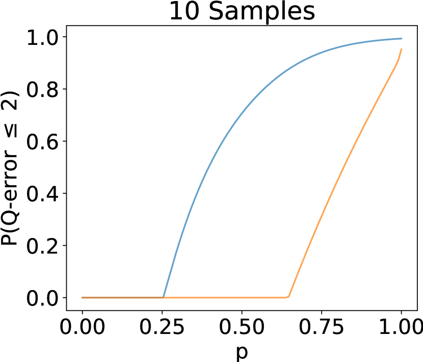
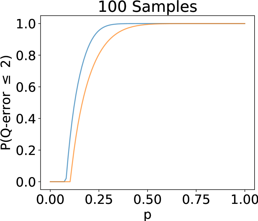
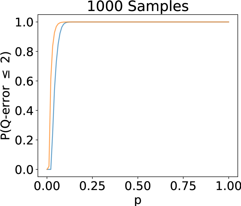
Figure 5: Comparing the Hoeffding-Serfling and Bernstein-Serfling bounds, assuming the length of the table is 1 billion.

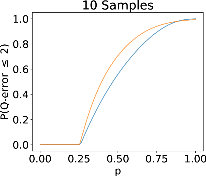
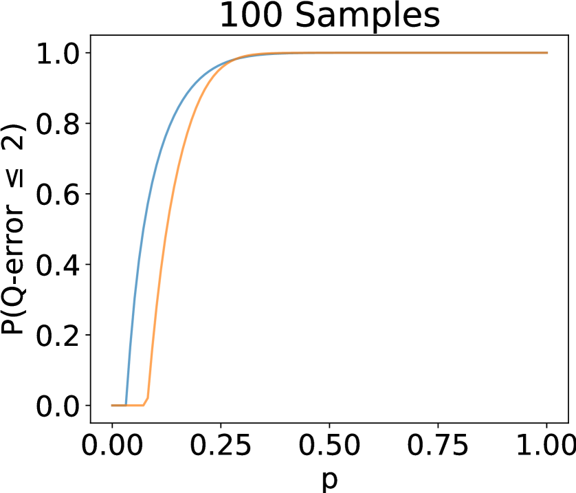
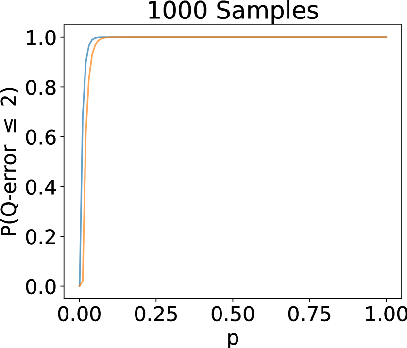
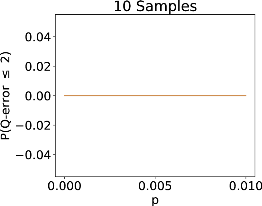
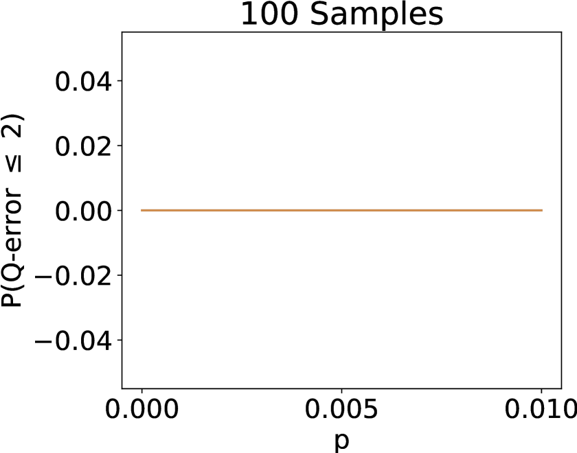
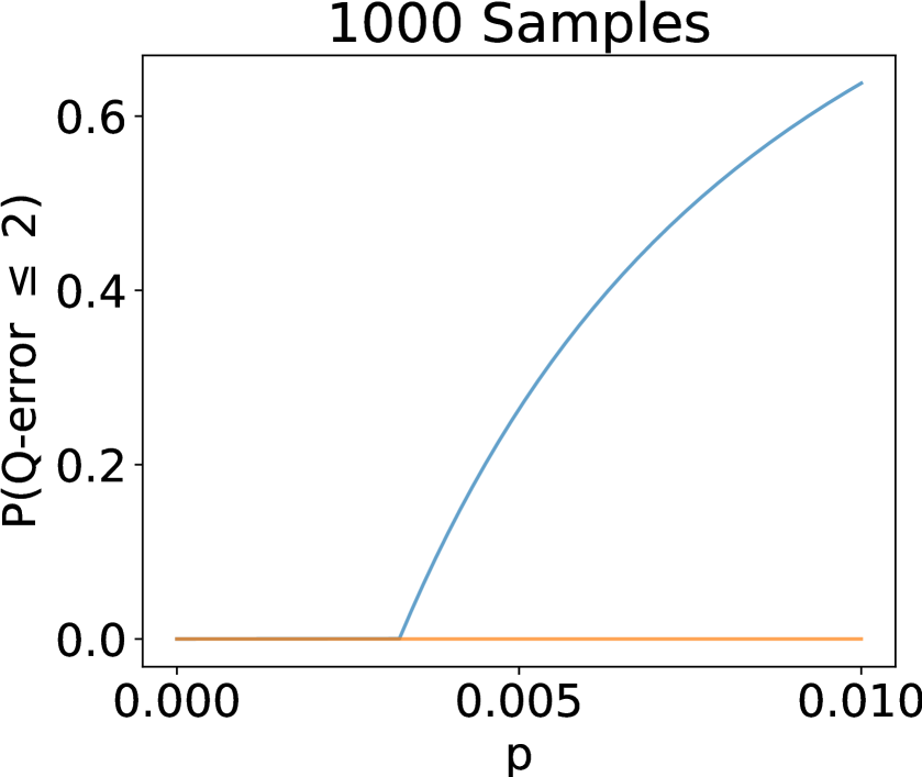
Figure 6: Comparing random uniform sampling with and without replacement at different cardinality values. Assume the length of the table is 1 billion.

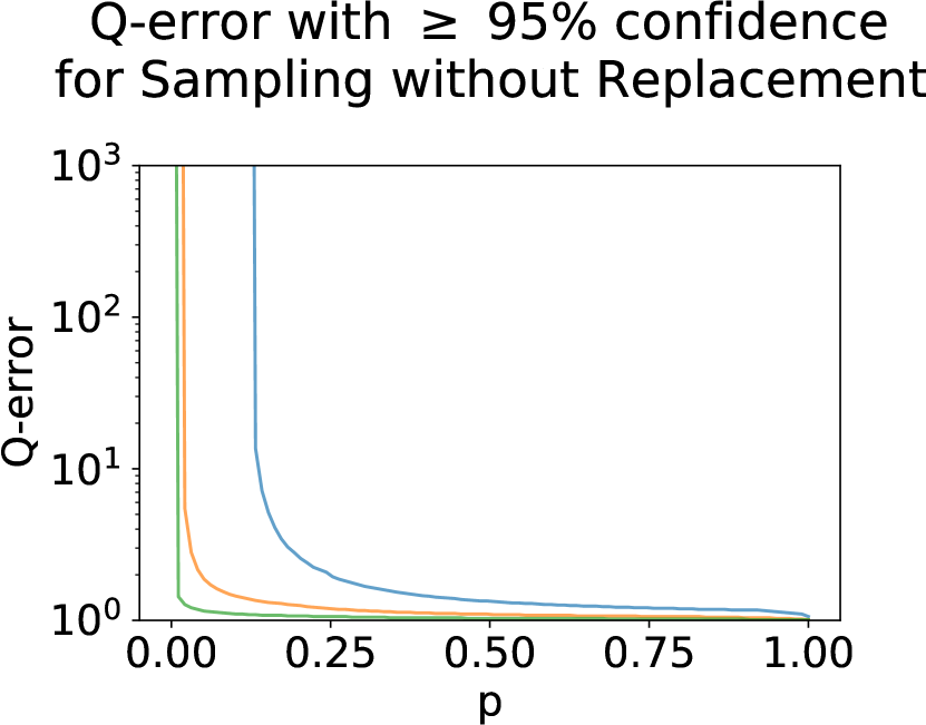
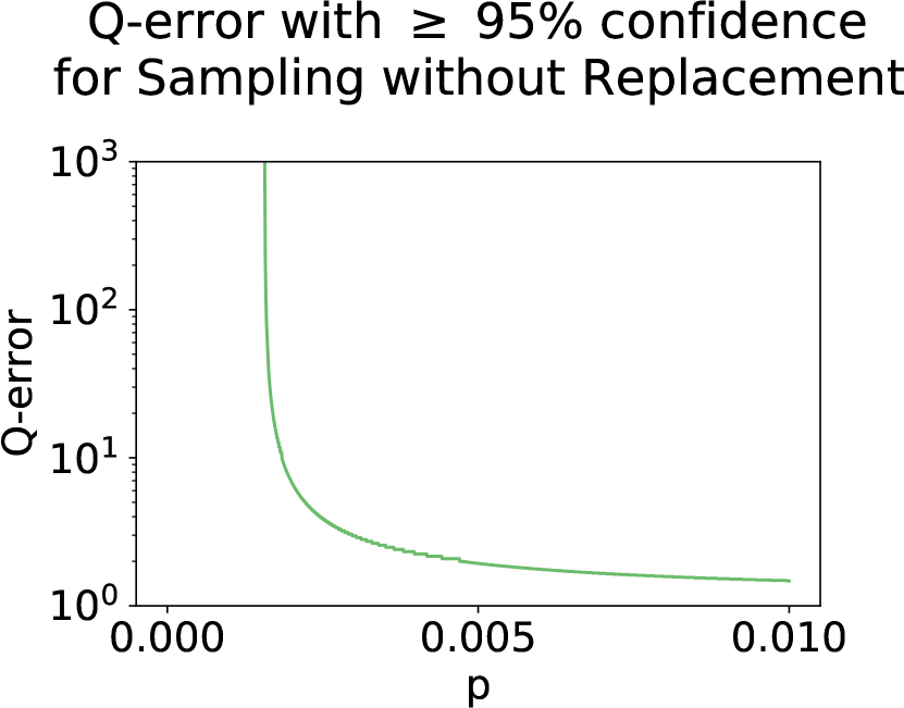
Figure 7: Plotting the Q-error with 95% confidence in terms of $p$. (Left) Results for $p\in(0,100\%]$. (Right) Results for $p\in(0,1\%]$.

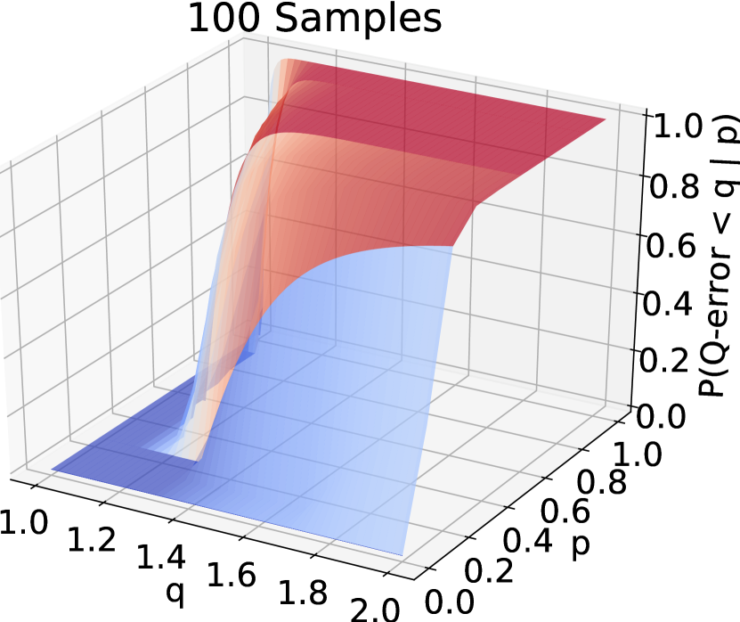
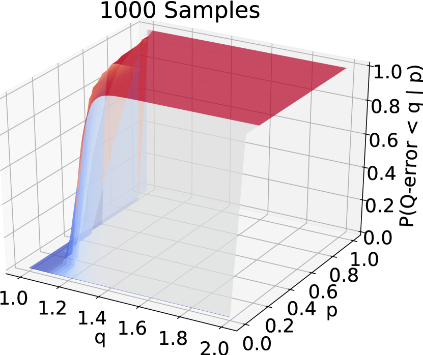
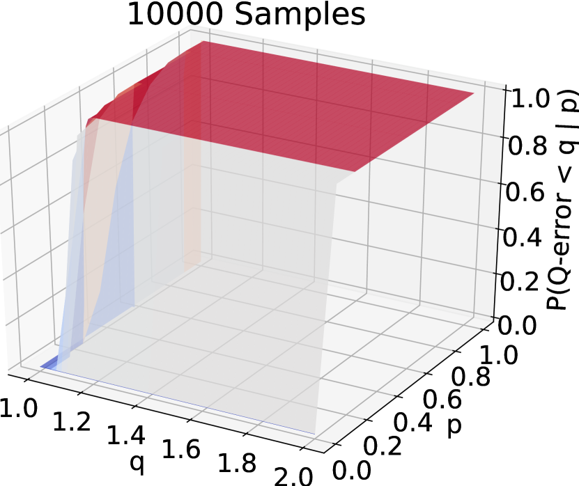
Figure 8: 3D plotting of the probability that random uniform sampling is better than $q$ at true cardinality $p$.

The analysis procedure using Bernstein-Serfling inequality is almost identical to the previous steps. Note there are two roots for $\delta$, but one root violates the constraint that $\cfrac{2\rho\log(1/\delta)}{k}\geq 0$.

$$\mathds{P}(Pred>qX) =\mathds{P}\Bigg{(}\frac{\sum\limits_{t=1}^{k}(X_{t}-p)}{k}>pq-p\Bigg{)}$$

(Let $$\delta=\exp\Big{(}-\frac{k}{\zeta^{2}}(-\sqrt{2\zeta\rho\sigma^{2}(pq-p)+\rho^{2}\sigma^{4}}+(pq-p)\zeta+\sigma^{2}\rho)\Big{)}$$)

$$=\mathds{P}\Bigg{(}\frac{\sum\limits_{t=1}^{k}(x_{t}-p)}{k}>\sigma\sqrt{\cfrac{2\rho\log(1/\delta)}{k}}+\cfrac{\zeta\log(1/\delta)}{k}\Bigg{)}$$

$$\leq 2\delta=2\exp\Big{(}-\frac{k}{\zeta^{2}}(-\sqrt{2\zeta\rho\sigma^{2}(pq-p)+\rho^{2}\sigma^{4}}+(pq-p)\zeta+\sigma^{2}\rho)\Big{)},$$

$$\mathds{P}(Pred<X/q) =\mathds{P}\Bigg{(}\frac{\sum\limits_{t=1}^{k}(Y_{t}-\bar{p})}{k}>p-p/q\Bigg{)}$$

( Let $$\delta=\exp\Big{(}-\frac{k}{\zeta^{2}}(-\sqrt{2\zeta\rho\sigma^{2}(p-p/q)+\rho^{2}\sigma^{4}}+(p-p/q)\zeta+\sigma^{2}\rho)\Big{)}$$ )

$$=\mathds{P}\Bigg{(}\frac{\sum\limits_{t=1}^{k}(Y_{t}-\bar{p})}{k}>\sigma\sqrt{\cfrac{2\rho\log(1/\delta)}{k}}+\cfrac{\zeta\log(1/\delta)}{k}\Bigg{)}$$

$$\leq 2\delta=2\exp\Big{(}-\frac{k}{\zeta^{2}}(-\sqrt{2\zeta\rho\sigma^{2}(p-p/q)+\rho^{2}\sigma^{4}}+(p-p/q)\zeta+\sigma^{2}\rho)\Big{)}.$$

Bound 4

By applying the Bernstein-Serfling Inequality, the Q-error of random uniform sampling without replacement is bounded by

$$\mathds{P}(\text{Q-error $\leq$ q}) =1-\mathds{P}(\text{Q-error $>$ q})$$

$$\geq 1-2\exp\Big{(}-\frac{k}{\zeta^{2}}(-\sqrt{2\zeta\rho\sigma^{2}(pq-p)+\rho^{2}\sigma^{4}}+(pq-p)\zeta+\sigma^{2}\rho)\Big{)}$$

$$-2\exp\Big{(}-\frac{k}{\zeta^{2}}(-\sqrt{2\zeta\rho\sigma^{2}(p-p/q)+\rho^{2}\sigma^{4}}+(p-p/q)\zeta+\sigma^{2}\rho)\Big{)}.$$

Putting together the $\Omega$ and $\Psi$ in the above bounds, we derive Theorem 4.

Visualization. Figure 5 plots and compares the bounds in this section. With 10K samples, the Q-error is almost always small ($q\leq$2) for both bounds. Figure 6 compares random uniform sampling with and without replacement at different $p$ values; we observe a tighter bound for random uniform sampling without replacement. Figure 7 shows the Q-error with at least 95% confidence at different $p$ values. Figure 8 shows the 3-D plotting of the probability that random uniform sampling is better than a given Q-error threshold. We also simulate and plot the results in Figure 9.

$p$	C	100 Samples		1000 Samples		10000 Samples
		R	NR	R	NR	R	NR
0.0002	166	0.00	0.00	0.00	0.00	0.00	0.00
0.0003	333	0.00	0.00	0.00	0.00	0.12	0.00
0.0005	500	0.00	0.00	0.00	0.00	0.39	0.00
0.0007	666	0.00	0.00	0.00	0.00	0.56	0.00
0.0008	833	0.00	0.00	0.00	0.00	0.68	0.00
0.0010	1000	0.00	0.00	0.00	0.00	0.76	0.00
0.0017	1666	0.00	0.00	0.00	0.00	0.92	0.42
0.0033	3333	0.00	0.00	0.12	0.00	0.99	0.85
0.0050	5000	0.00	0.00	0.39	0.00	1.00	0.96
0.0067	6666	0.00	0.00	0.56	0.00	1.00	0.99
0.0083	8333	0.00	0.00	0.68	0.00	1.00	1.00
0.0100	10000	0.00	0.00	0.76	0.00	1.00	1.00
0.1667	166666	0.92	0.75	1.00	1.00	1.00	1.00
0.3333	333333	0.99	1.00	1.00	1.00	1.00	1.00
0.5000	500000	1.00	1.00	1.00	1.00	1.00	1.00
0.6667	666666	1.00	1.00	1.00	1.00	1.00	1.00
0.8333	833333	1.00	1.00	1.00	1.00	1.00	1.00
1.0000	1000000	1.00	1.00	1.00	1.00	1.00	1.00

Table 1: Confidence that Q-error is at most 2 from Theorem 3 and Theorem 4. Assuming there are 1 million rows, we provide ratio $p$ and the cardinality (C). R = Sampling with Replacement. NR = Sampling without Replacement. $1.00$ is rounded from values that is greater than $0.995$.

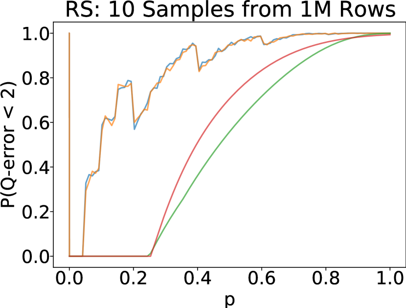
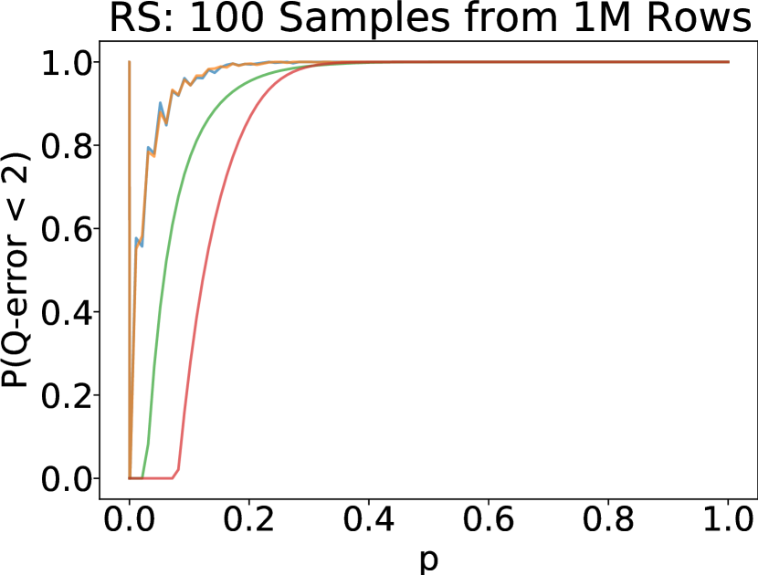
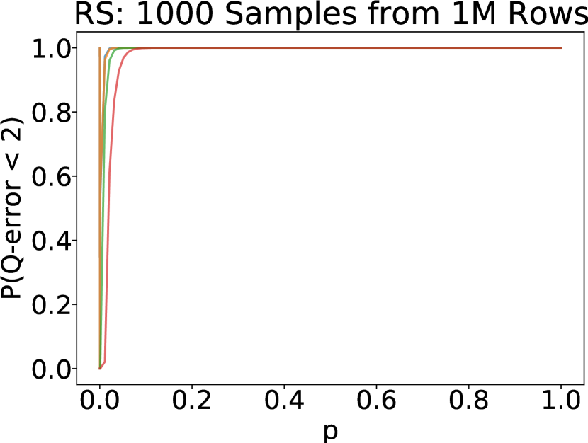
Figure 9: For each point in the figure, we conducted a simulation for 1,000 times and plotted the simulation results with Theorem 3 and Theorem 4 assuming 1 million rows in the table. When $k$ is small, our bounds are conservative. At a slightly larger $k$, our bounds are tight compared to the simulations.

5 Related Work

Recently, [7] applied random uniform sampling to dynamically modify the sample size $k$ used in machine learning model training. Their approach can achieve $\epsilon$-optimally by a novel approximation algorithm with Chernoff bound and Hoeffding’s inequality. The authors change the sample size $k$ based on the number of satisfied rows in the samples. In this paper, we fix the sample size $k$ and analyze the bound of the Q-error, assuming the ground truth $p$ is known but the number of satisfied rows is unknown. These two analyses may result in different applications. In another study, [19] calculated the expected Q-error for TPC-H and several other datasets when the cardinality is extremely small. They also created a novel algorithm that can reduce the expected Q-error. Our analysis in this paper provides confidence intervals other than expected accuracy.

6 Conclusion

In this paper, we apply different statistical tools to analyze the upper Q-error bounds of random uniform sampling for single-table cardinality estimation. Our analysis indicates that a simple sampling already provides robust estimates when the true cardinality is relatively high (e.g., at 1000 rows, $>1\%$ selectivity).

It is easy to see that our analysis in this paper can be extended to sample-based CE after join. Using small samples for each join relation may yield a good error bound; however, deciding which join relations to materialize is an open question. For join on samples, we refer the readers to recent analyses in [14].

Appendix

For cardinality estimation over single tables, the Q-error of random uniform sampling with replacement is bounded by

$$\mathds{P}(\text{Q-error $\leq$ q})\geq 1-\Omega-\Psi,where$$

$$\Omega =\min\Bigg{(}\Big{(}\cfrac{e^{q-1}}{q^{q}}\Big{)}^{pk},\exp\Big{(}-\frac{k(pq-p)^{2}}{2\sigma^{2}+2(pq-p)/3}\Big{)},exp\Big{(}-2p^{2}(q-1)^{2}k\Big{)}\Bigg{)},$$

$$\text{when~{}}pq>1,\Psi =\min\Bigg{(}\Big{(}e^{(\frac{1}{q}-1)}q^{\frac{1}{q}}\Big{)}^{pk},\exp\Big{(}-\frac{k(p-p/q)^{2}}{2\sigma^{2}+2(p-p/q)/3}\Big{)},exp\Big{(}-\frac{2k(pq-1)^{2}}{q^{2}}\Big{)}\Bigg{)},$$

$$\text{when~{}}pq\leq 1,\Psi =\min\Bigg{(}\Big{(}e^{(\frac{1}{q}-1)}q^{\frac{1}{q}}\Big{)}^{pk},\exp\Big{(}-\frac{k(p-p/q)^{2}}{2\sigma^{2}+2(p-p/q)/3}\Big{)}\Bigg{)}.$$

The Hoeffding’s inequality can be written as the following inequalities, where $\epsilon>0$:

$$\mathds{P}(\hat{X}\geq(p+\epsilon)k)\leq exp(-2\epsilon^{2}k),$$ (4)

$$\mathds{P}(\hat{X}\leq(p-\epsilon)k)\leq exp(-2\epsilon^{2}k).$$ (5)

We can improve Theorem 3 by adding Hoeffding’s inequality. The bound provided below requires $pq>1$ for under-estimation and we excluded it from Theorem 3 for simplicity.

$$\mathds{P}(Pred\geq qX) =\mathds{P}(\hat{X}\geq q\mu)$$

(Let $$\epsilon=qp-p$$)

$$\leq exp(-2p^{2}(q-1)^{2}k).$$

$$\mathds{P}(Pred\leq\frac{1}{q}X) =\mathds{P}(\hat{X}\leq\frac{1}{q}\mu)$$

(Let $$\epsilon=p-\frac{1}{q} pq>1$$ and )

$$\leq exp(-\frac{2k(pq-1)^{2}}{q^{2}})\text{~{}~{}~{}~{}~{}(if $pq>1$)}.$$

Bound 5

By Hoeffding’s inequality, when $pq>1$, random sampling with replacement has the Q-error bound

$$\mathds{P}(\text{Q-error $<$ q})\geq 1-exp(-2p^{2}(q-1)^{2}k)-exp(-\frac{2k(pq-1)^{2}}{q^{2}}).$$

References

• [1] R. Bardenet, O.-A. Maillard, et al. Concentration inequalities for sampling without replacement. Bernoulli, 21(3):1361–1385, 2015.
• [2] K. S. Beyer, P. J. Haas, B. Reinwald, Y. Sismanis, and R. Gemulla. On synopses for distinct-value estimation under multiset operations. In SIGMOD, 2007.
• [3] N. Bruno, S. Chaudhuri, and L. Gravano. STHoles: A multidimensional workload-aware histogram. SIGMOD, 2001.
• [4] G. Cormode, M. Garofalakis, P. J. Haas, and C. Jermaine. Synopses for massive data: Samples, histograms, wavelets, sketches. Found. Trends databases, 4, Jan. 2012.
• [5] G. Cormode and S. Muthukrishnan. An improved data stream summary: The count-min sketch and its applications. J. Algorithms, 2005.
• [6] M. Durand and P. Flajolet. Loglog counting of large cardinalities. In ESA, 2003.
• [7] A. Dutt, C. Wang, V. Narasayya, and S. Chaudhuri. Efficiently approximating selectivity functions using low overhead regression models. Proceedings of the VLDB Endowment, 13(12):2215–2228, 2020.
• [8] A. Dutt, C. Wang, A. Nazi, S. Kandula, V. Narasayya, and S. Chaudhuri. Selectivity estimation for range predicates using lightweight models. Proceedings of the VLDB Endowment, 12(9):1044–1057, 2019.
• [9] B. Efron and R. Tibshirani. Bootstrap methods for standard errors, confidence intervals, and other measures of statistical accuracy. Statistical science, pages 54–75, 1986.
• [10] P. Flajolet and G. N. Martin. Probabilistic counting algorithms for data base applications. J. Comput. Syst. Sci., 1985.
• [11] P. J. Haas, J. F. Naughton, S. Seshadri, and L. Stokes. Sampling-based estimation of the number of distinct values of an attribute. In VLDB, volume 95, pages 311–322, 1995.
• [12] P. J. Haas, J. F. Naughton, S. Seshadri, and A. N. Swami. Selectivity and cost estimation for joins based on random sampling. J. Comput. Syst. Sci., 52(3), 1996.
• [13] B. Hilprecht, A. Schmidt, M. Kulessa, A. Molina, K. Kersting, and C. Binnig. Deepdb: Learn from data, not from queries! arXiv preprint arXiv:1909.00607, 2019.
• [14] D. Huang, D. Y. Yoon, S. Pettie, and B. Mozafari. Joins on samples: A theoretical guide for practitioners. VLDB, 2021.
• [15] Y. Ioannidis. The history of histograms (abridged). VLDB, 2003.
• [16] A. Kipf, T. Kipf, B. Radke, V. Leis, P. Boncz, and A. Kemper. Learned cardinalities: Estimating correlated joins with deep learning. arXiv preprint arXiv:1809.00677, 2018.
• [17] B. Li, Y. Lu, C. Wang, and S. Kandula. Cardinality estimation: Is machine learning a silver bullet? In 3rd International Workshop on Applied AI for Database Systems and Applications (AIDB), 2021.
• [18] G. S. Manku and R. Motwani. Approximate frequency counts over data streams. In VLDB, 2002.
• [19] G. Moerkotte and A. Hertzschuch. alpha to omega: the g (r) eek alphabet of sampling. In CIDR, 2020.
• [20] W. Mulzer. Five proofs of chernoff’s bound with applications. arXiv preprint arXiv:1801.03365, 2018.
• [21] Z. Yang, E. Liang, A. Kamsetty, C. Wu, Y. Duan, X. Chen, P. Abbeel, J. M. Hellerstein, S. Krishnan, and I. Stoica. Deep unsupervised cardinality estimation. arXiv preprint arXiv:1905.04278, 2019.