Time-aware Path Reasoning on Knowledge Graph for Recommendation

Abstract.

Reasoning on knowledge graph (KG) has been studied for explainable recommendation due to its ability of providing explicit explanations. However, current KG-based explainable recommendation methods unfortunately ignore the temporal information (such as purchase time, recommend time, etc.), which may result in unsuitable explanations. In this work, we propose a novel Time-aware Path reasoning for Recommendation (TPRec for short) method, which leverages the potential of temporal information to offer better recommendation with plausible explanations. First, we present an efficient time-aware interaction relation extraction component to construct collaborative knowledge graph with time-aware interactions (TCKG for short), and then introduce a novel time-aware path reasoning method for recommendation. We conduct extensive experiments on three real-world datasets. The results demonstrate that the proposed TPRec could successfully employ TCKG to achieve substantial gains and improve the quality of explainable recommendation.

1. Introduction

Recently, knowledge graphs (KGs) have been widely used in recommender systems due to their rich structured knowledge (e.g., (Wang et al., 2018c; Xian et al., 2019; Zhang et al., 2016; Wang et al., 2018d; Huang et al., 2018; Wang et al., 2018b; Zhao et al., 2020; Wu et al., 2021; Zeng et al., 2022; Wang et al., 2019b)). A KG is a type of directed heterogeneous graph in which nodes represent real-world entities and edges represent their relations. Reasoning over KGs (Xian et al., 2019; Zhao et al., 2020) for recommendation can not only infer user preferences more accurately, but also offer each recommended item with a multi-hop path. Such knowledge-aware paths allow us to explain why an item is recommended, so as to increase users’ satisfaction and trust (Tintarev and Masthoff, 2007b, a). Existing methods adopt reinforcement learning agents to automatically mine and reason over such paths. The core lies in using ”What items will users purchase?” to guide the reasoning process towards the target items.

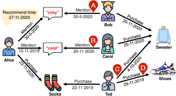
Figure 1. Example of how temporal information assists in explainable recommendation.

However, current RL agents mostly treat the user-item interaction as the static relation, and ignore the time-aware information of interactions (e.g., purchase time). Hence, they fall short in modeling the temporal patterns of user behaviors, possibly offering unreliable reasoning paths and recommendations. Considering the example in Figure 1, where A, B, C and D marked in red indicate different reasoning paths. Typical KG reasoning methods (e.g., (Xian et al., 2019; Zhao et al., 2020)) may recommend $Sweater$ to $Alice$, which can be explained by the path A existing in the corresponding KG, namely, $Alice\stackrel{{\scriptstyle Mention}}{{\longrightarrow}}\text{cozy}\stackrel{{\scriptstyle Mentioned\_by}}{{\longrightarrow}}Bob\stackrel{{\scriptstyle Purchase}}{{\longrightarrow}}Sweater$. However, with the help of temporal information, it can be shown that the reasoning paths B and D are better than A and C. First, in explaining the same recommendation $Sweater$, path B is more reasonable than A since its relation time (10-11-2019) is in the season of winter, which is consistent with the recommendation time (27-11-2020). This implies the periodic patterns of user behaviors. Second, path D is better than C since the purchase time 29-11-2019 and recommendation time 27-11-2020 are both Black Friday while 4-10-2020 is closer to 27-11-2020 only in linear time. People tend to have similar behaviors in shopping festivals. In this sense, we consider Path D a better recommendation. Therefore, a time-aware KG reasoning method is more likely to generate better recommendation results.

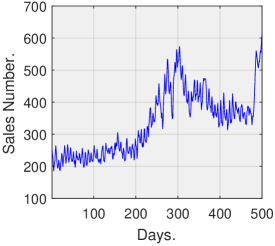
(a) Clothing

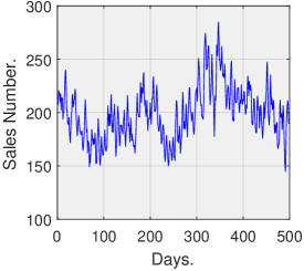
(b) Cell Phones.

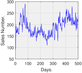
(c) Beauty

Figure 2. Sales behavior in three Amazon datasets.

While some KG-based recommendation methods have modeled temporal information (Wang et al., 2020; Huang et al., 2018, 2019), they mainly use KG data to enhance representation rather reasoning over the KG. Their focus is on modeling the interaction sequence for sequential recommendation, rather than the more general temporal patterns as exampled above. It remains underexplored how to model the rich patterns (e.g., seasons, shopping festivals, etc.) that can be inferred from timestamps.

In this work, we frame user-item interactions as time-aware relations. In the example of Figure 1, if the reasoning agent is guided by ”What items will users purchase in winter and festival?” , then Path B and Path D can be easily inferred. Nonetheless, it is non-trivial due to the following challenges: (i) A huge number of timestamps. Figure 2 is based on the Amazon datasets (He and McAuley, 2016), which demonstrate user purchasing behaviors, as well as the corresponding timestamps over a 500-day period. As the total number of timestamps is numerous, they cannot be directly considered as relation types. (ii) Ambiguous definition of temporal distance. Those timestamps do not always suggest similar user behaviors. As illustrated in Figure 2, the sales of items in the same season tend to be similar in different years, rather than in different seasons of the same year. (iii) Different information sources. In recommender systems, the interactions between users and items continuously stream in. But the external KG is relatively stable and seldom updated, which means we couldn’t treat them equally when performing time-aware path reasoning.

To address the above challenges, we integrate the time-aware interactions into KG as a heterogeneous information graph (TCKG for short). We propose a novel Time-aware Path reasoning for Recommendation (TPRec for short) method. Our method consists of three components. The first one is the time-aware interaction relation extraction component. We apply time series clustering on the interaction timestamps and replace the original interaction relations with clustered relations. By doing this, we could control the number of relation types, and make the extracted relations sensitive to time. More specifically, the timestamp’s temporal features consist of statistical and structural discriminative properties, which enables us to measure temporal similarity and behavioral pattern similarity. In the second component, we adopt translational distance learning to encode entities and relations in TCKG to obtain time-aware semantic representation. The third component is the key time-aware path reasoning component. In this component, we shape a personalized time-aware reward based on each user’s interaction history and recommend time, which is used to guide the reinforcement learning (RL) reasoner to explore more precisely.

In summary, the contributions are as follows:

• We design a TCKG to properly integrate the temporal information into KG-based recommendation. To the best of our knowledge, it is the first work to introduce time-aware path reasoning for explainable recommendation.

• We propose a personalized time-aware reward to guide the RL-based reasoning agent, which makes the time-aware reasoning achieve a more accurate and interpretable recommendation.

• We conduct experiments on three real-world datasets, and the results demonstrate the effectiveness of TPRec over several state-of-the-art baselines. The codes are available at https://github.com/Go0day/TPRec.

2. Problem Formulation

Table 1. Notation and Definitions.

Notations	Annotation
$\mathcal{U}$	User set
$\mathcal{V}$	Global item set
$\mathcal{V}_{\mathcal{U}}$	The observed interactions between users and items
$\mathcal{V}_{\mathcal{U}}^{T}$	The clustered time-aware interaction set, with $L$ categories
$\mathcal{G}_{T}$	Time-aware Collaborative Knowledge Graph
$\mathcal{E}^{\prime}$	The entities in Time-aware Collaborative Knowledge Graph
$\mathcal{R}_{T}$	The relations in Time-aware Collaborative Knowledge Graph
$T$	The interaction timestamp set
$\hat{T}$	The recommend time
$\hat{\mathcal{V}}$	The recommended item set
$\tau_{u,\hat{\mathcal{V}}}$	The reasoning path set for user $u$ to item set $\hat{\mathcal{V}}$
$\mathcal{T}$	Temporal feature space, including statistical features and structural features
$r_{kg}$	The external knowledge graph relation set
$r_{interact}$	The time-aware interaction relation set
r	The embedding of relations
$\textbf{e}_{h},\textbf{e}_{t}$	The embedding of entities
$\textbf{W}_{t},\textbf{W}_{\hat{T}}$	The weight distribution of the Gaussian models at timestamp $t$, $\hat{T}$
$\textbf{W}_{h_{u}}$	The time cluster weight distribution of user $u$’s interaction history
$k,k^{\prime},K$	The $k$-th reasoning step, state history length $k^{\prime}$ and terminal step
$\textbf{s}_{k}$	The state at step $k$
$a_{k},\mathcal{A}_{k}$	The action and action space at step $k$
$g_{R}(\hat{v}\mid u)$	The time-aware based reward for recommended item $\hat{v}$ for user $u$
$\pi\left(\cdot\mid\mathbf{s}_{k},\mathcal{A}_{k}(u)\right)$	The policy network at step $k$
$\hat{c}(\mathbf{s}_{k})$	The value network at step $k$

Notions: We consider the time-aware path reasoning for KG-enhanced recommendation. Let denote the user set, the item set, and the observed interactions as $\mathcal{U}$, $\mathcal{V}$, ${\mathcal{V}}_{\mathcal{U}}$, respectively. Moreover, there exists an external KG storing item properties. Generally, the KG is represented as $\mathcal{G}=\{(h,r,t)\mid h,t\in\mathcal{E},r\in\mathcal{R}\}$, where $\mathcal{E}$ represents the set of real-world entities and $\mathcal{R}$ is the set of relation. Each triplet $(h,r,t)$ delineates that there exist a relationship $r$ from head entity $h$ to tail entity $t$. Previous works (Sun et al., 2020; Wang et al., 2019a) combine the user behaviors and item knowledge as a unified relational graph, termed Collaborative Knowledge Graph (CKG), which is defined as $\mathcal{G}_{R}=\{(h,r,t)\mid h,t\in\mathcal{E}^{\prime}$, $r\in\mathcal{R}^{\prime}\}$, where $\mathcal{E}^{\prime}=\mathcal{E}\cup\mathcal{U}$ and $\mathcal{R}^{\prime}=\mathcal{R}\cup{\mathcal{V}}_{\mathcal{U}}$. The notations of this work are summarized in Table 1.

Reasoning Environment: Considering the time-aware interactions instead, we further obtain a Time-aware Collaborative Knowledge Graph (TCKG), which is the environment of time-aware path reasoning. Specifically, the interaction timestamps are grouped into $L$ groups after time-series clustering, and the interaction relation ${\mathcal{V}}_{\mathcal{U}}$ is extended to $\{\mathcal{V}_{\mathcal{U}}^{1},\mathcal{V}_{\mathcal{U}}^{2},\cdots,\mathcal{V}_{\mathcal{U}}^{L}\}$. Hence, the TCKG is formulated as $\mathcal{G}_{T}=\{(h,r,t)\mid h,t\in\mathcal{E}^{\prime},r\in\mathcal{R}_{T}\}$, where $\mathcal{R}_{T}=\mathcal{R}\cup\{\mathcal{V}_{\mathcal{U}}^{1},\mathcal{V}_{\mathcal{U}}^{2},\cdots,\mathcal{V}_{\mathcal{U}}^{L}\}$.

Task Description: We present the task of time-aware path reasoning for recommendation (TPRec) as follows:

• Input: Time-aware collaborative knowledge graph $\mathcal{G}_{T}$;

• Output: Given a user $u$ and a timestamp $\hat{T}$, a recommender model results in an item set $\hat{\mathcal{V}}\subseteq\mathcal{V}$ with the corresponding explainable reasoning paths $\tau_{u,\hat{\mathcal{V}}}$. In particular, for an item $\hat{v}\in\hat{\mathcal{V}}$, $\tau_{u,\hat{v}}$ is a multi-hop path, which connects user $u$ with item $\hat{v}$ to explain why $\hat{v}$ is suitable for $u$: $\tau_{u,\hat{v}}=[u\stackrel{{\scriptstyle r_{1}}}{{\longrightarrow}}e_{1}\stackrel{{\scriptstyle r_{2}}}{{\longrightarrow}}\ldots\stackrel{{\scriptstyle r_{k-1}}}{{\longrightarrow}}e_{k-1}\stackrel{{\scriptstyle r_{k}}}{{\longrightarrow}}\hat{v}]$, where $e_{i-1}\stackrel{{\scriptstyle r_{i}}}{{\longrightarrow}}e_{i}$ represents $(e_{i-1},r_{i},e_{i})\in\mathcal{G}_{T},i\in[k]$.

3. Methodology

In this section, we introduce the proposed TPRec in detail. The overall framework of time-aware path reasoning is shown in Figure 4. Our approach is able to effectively fuse temporal information into knowledge graph and leverage a RL framework for recommendation. In what follows, we start with Time-aware Interaction Relation Extraction to construct TCKG, and use Time-aware representation learning to generate entities and relations representations. Then we present Time-aware Path Reasoning and Model Prediction to reason over TCKG for recommendation.

3.1. Time-aware Interaction Relation Extraction

Clearly, how to deal with the dynamic characteristics of user-item interactions is of crucial importance in our task. However, simply treating the interaction timestamps as auxiliary features might limit the potential of time-aware reasoning, due to the following challenges: (1) As the timestamps are usually numerous (Ni et al., 2019), directly attaching them with user behaviors might cause meaningless features, such as purchase_20150101 and purchase_20150102, thus enlarging the feature space dramatically and losing the periodic semantics of timestamps. (2) The interaction graph and knowledge graph come from heterogeneous sources, and thus are hardly updated synchronously — that is, the interactions are usually dynamic, while the item knowledge (e.g., category, brand) is fixed over different timestamps.

To solve these challenges, we first consider the temporal and behavioral characteristics of interactions by projecting the timestamps into a temporal feature space $\mathcal{T}$. It encodes temporal statistical and temporal structural features of interaction timestamps. We then group the interaction timestamps $T=\{t_{1},t_{2},\cdots,t_{n}\}$ into $L$ categories, and then extend the single interaction type into $\mathcal{V}_{\mathcal{U}}^{T}=\{\mathcal{V}_{\mathcal{U}}^{1},\mathcal{V}_{\mathcal{U}}^{2},\cdots,\mathcal{V}_{\mathcal{U}}^{L}\}$. After that, the temporal user-item graph can be seamlessly integrated with relatively static KG based on the item-entity alignment set, and finally get the TCKG we need. The extraction process is illustrated in Figure 3.

3.1.1. Temporal Statistical Features

Before clustering timestamps, we project them into a feature space. Specifically, the statistical features are considered to capture some time rules like seasonal changes, periodic purchases (Liao, 2005). Hence, for a specific timestamp $t$, its statistical feature is formally summarized as:

(1) $$\bm{f}_{stat}=year(t)||season(t)||month(t)||week(t)\cdots,$$

where $\bm{f}_{stat}$ encodes the year, season, month, week, and other statistical characteristics of $t$ and concatenates them together, where $||$ is the concatenate operator.

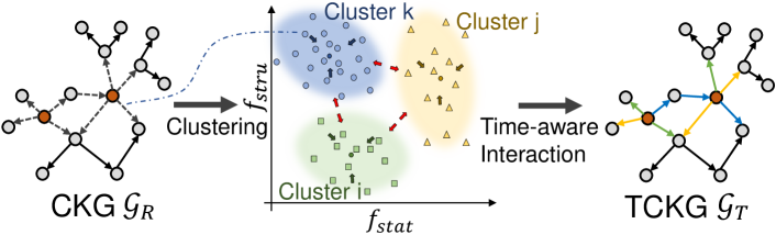
Figure 3. Process of time-aware interaction relation extraction. Each interaction relation’s (dashed edge) timestamp will be mapped into temporal feature space $\mathcal{T}$ and clustered. Different colored edges (e.g., blue, yellow, green) in TCKG represent different clustering results.

3.1.2. Temporal structural features

Beyond the statistical features, we also exploit the structural features to delineate the characteristics of user behaviors, which measures the purchase propensity (e.g., shopping festival) at timestamp $t$. More formally, we define the structural feature of $t$ as:

(2) $$\bm{f}_{stru}=z_{gap}^{\prime}(t)||z_{gap}^{\prime\prime}(t),$$

where $z_{gap}^{\prime}(t)$ is the first-order structural feature, which measures the trend of interaction number in the current $gap$ time, compared with that in the past $gap$; $gap$ represents the granularity of window period, which can be set as 30 (i.e., month), or 1 (i.e., day); analogously, $z_{gap}^{\prime\prime}(t)$ denotes the second-order structural feature and models the momentum of interaction trend. More formally, $z_{gap}^{\prime}(t)$ and $z_{gap}^{\prime\prime}(t)$ is defined as:

(3) $$z_{gap}^{\prime}(t) =\frac{\sum_{i=t-gap}^{t}z(i)-\sum_{i=t-2gap}^{t-gap}z(i)}{gap},\ z_{gap}^{\prime\prime}(t) =\frac{\sum_{i=t-gap}^{t}z_{gap}^{\prime}(i)-\sum_{i=t-2gap}^{t-gap}z_{gap}^{\prime}(i)}{gap},$$

where $z(i)$ is the interaction number happened on timestamp $i$, and we replace $z(i)$ with $z_{gap}^{\prime}(i)$ in Eq. 3 to calculate $z_{gap}^{\prime\prime}(t)$. For those timestamp $t$ has less than $2gap$ historical interactions, their historical information is not enough to calculate $z_{gap}^{\prime}(i)$. In that case, we padding their corresponding features with the nearest timestamp’s temporal structural feature. The same goes for $z_{gap}^{\prime\prime}(t)$. In this work, we set the gap as 90 (i.e., season), 30 (i.e., month), 7 (i.e., week), 1 (i.e., day) and simply concatenate them as temporal structural features.

Thereafter, we combine these two features together as the temporal feature space $\mathcal{T}\in\mathbb{R}^{m}$ for timestamp $t$:

(4) $$\mathcal{T}=\bm{f}_{stat}\ ||\ \bm{f}_{stru},$$

where $m$ is the feature dimension.

3.1.3. TCKG Construction

Having mapped the timestamp to the temporal feature space, we now construct the relation of time-aware interaction. Here we adopt a time-series clustering method, Gaussian Mixture Model (GMM) (Reynolds, 2009), on the timestamp set $T$, so as to reduce the timestamp numbers and discretize them into group values. We leave the exploration of other clustering methods, such as K-means (Kanungo et al., 2002), DBSCAN (Ester et al., 1996), and Mean-shift (Comaniciu and Meer, 2002), in future work.

Specifically, we hire $L$ Gaussian models. For the timestamp $t$ with its temporal feature, we can get the probability $w_{l}$ of being generated by the $l$-th Gaussian model. As such, the interaction relation $r_{t}$ on timestamp $t$ can be obtained as follows:

(5) $$r_{t}\leftarrow\mathbb{I}_{max(\textbf{W}_{t})}(\textbf{W}_{t}){\mathcal{V}_{\mathcal{U}}^{T}}\ ,$$

where $\textbf{W}_{t}=[w^{1}_{t},w^{2}_{t},\cdots,w^{L}_{t}]^{\mathsf{T}}$ indicates the $t$-specific probability distribution derived from the Gaussian models; ${\mathcal{V}}_{\mathcal{U}}^{T}=[\mathcal{V}_{\mathcal{U}}^{1},\mathcal{V}_{\mathcal{U}}^{2},\cdots,\mathcal{V}_{\mathcal{U}}^{L}]$ is the time-aware interaction relation set, where $\mathcal{V}_{\mathcal{U}}^{l}$ is the $l$-th clustered relation. Equation (5) replaces $r_{t}$ with the most probable relation in ${\mathcal{V}}_{\mathcal{U}}^{T}$. The number of time clusters $L$ is determined by the Bayesian Information Criterion (BIC) (Vrieze, 2012), which is adjusted adaptively for different datasets.

Through the above extract process, we are able to project each observed interaction with timestamp into the same time-aware feature space, and divide all timestamps into weighted $L$ clusters by GMM. The clustering assignments are used to replace the original interaction relations in CKG and finally convert CKG into TCKG.

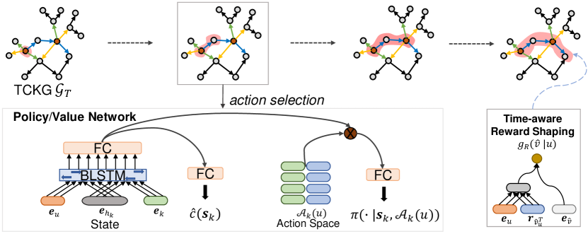
Figure 4. Overall training approach of the proposed TPRec model. For a user $u$ at each time step $k$, as shown in the pink shaded part of TCKG, the agent chooses the next hop based on the temporal constraint, which samples a link $a_{k}$ according to $\pi\left(\cdot\mid\mathbf{s}_{k},\mathcal{A}_{k}(u)\right)$. The agent receives a reward $g_{R}(\hat{v}\mid u)$ when stopped at an item $\hat{v}$. The pink shaded path starts at user $u$ and ends at item $\hat{v}$, showing why our TPRec model recommends $\hat{v}$ to $u$.

3.2. Time-aware Representation Learning

Having constructed TCKG, we aim to learn representations for entities and relations by exhibiting the structural and temporal information. In particular, the KG relations (defined as $r_{kg}$) require the entity representations to meet the structural constraints and maintain the semantics, while the time-aware interaction relations (defined as $r_{interact}\in{\mathcal{V}}_{\mathcal{U}}^{T}$) encourage the relation affinity within the same categories compared to that of different categories.

Towards this end, we employ the widely-used knowledge graph embedding method, TransE (Bordes et al., 2013), on TCKG. To be more specific, for a given TCKG triplet $(h,r,t)$, it represents head entity $h$, relation $r\in\{r_{kg}\cup r_{interact}\}$ , and tail entity $t$ with $d$-dimension embeddings, i.e., $\textbf{e}_{h}$, r, $\textbf{e}_{t}$ $\in\mathbb{R}^{d}$. These embeddings follow the translational principle: $\textbf{e}_{h}+\textbf{r}\approx\textbf{e}_{t}$. Hence, for a given triplet $(h,r,t)$, the scoring function is defined as the distance between $\textbf{e}_{h}+\textbf{r}$ and $\textbf{e}_{t}$, i.e.,

(6) $$g_{r}({h},{t})=\|\textbf{e}_{h}+\textbf{r}-\textbf{e}_{t}\|_{2}^{2}.$$

A smaller score $g_{r}(h,t)$ suggests that the fact $(h,r,t)$ is more likely to be true, and vice versa. We employ the pairwise loss function to train the TCKG embeddings, which accounts for the relative order between the valid triplets and broken ones:

(7) $$\mathbf{\mathop{\mathcal{L}}}_{tckg}=\sum_{\left(h,r,t,t^{\prime}\right)\in\mathcal{S}}-\ln\sigma\left(g_{r}({h},{t}^{\prime})-g_{r}({h},{t})\right)$$

where $\mathcal{S}=\{(h,r,t,t^{\prime})|(h,r,t)\in\mathcal{G}_{T},(h,r,t^{\prime})\notin\mathcal{G}_{T}\}$, and $(h,r,t^{\prime})$ is collected with the tail $t$ replaced by a random entity $t^{\prime}$; $\sigma(\cdot)$ is the sigmoid function. This loss serves as a constraint that injects the structural and temporal information into representations, thus preserving the semantics of entities and relations.

3.3. Time-aware Path Reasoning

Having established the embeddings of entities and relations, we feed them into the Time-aware Path Reasoning module. We utilize path reasoning to identify a set of recommended items $\hat{\mathcal{V}}$ for each user $u$ as well as reasoning paths $\{\tau_{u,\hat{v}}|\hat{v}\in\hat{\mathcal{V}}\}$ for the recommendation. Nonetheless, existing path reasoning models (Xian et al., 2019; Zhao et al., 2020) fail to consider temporal information, which might hurt the recommendation performance and result in improper explanations (as illustrated in Figure 1). To solve this issue, we introduce temporal information by setting personalized time-aware reward during path reasoning.

3.3.1. Markov Decision Process Formulation

We follow the previous studies and use the Markov Decision Process (MDP) (Sutton and Barto, 2018) in reinforcement learning (RL) to set up the reasoning environment. The environment can (1) inform the reasoner about its search state and available actions in the TCKG, and (2) reward the reasoner how well the current policy fits the observed user interactions. Overall, the MDP consists of the following components:

State. The initial state is $\textbf{s}_{0}=(u,u,\varnothing)$, and the state at step $k$ is $\textbf{s}_{k}=(u,h_{k},e_{k})$, where $u\in\mathcal{U}$ denotes the initial user entity, $e_{k}$ is the entity which the agent has reached at step $k$, and $h_{k}$ is the history prior to step $k$. Moreover, to control the model size, we adopt $k^{\prime}$-step history to encode the combination of all entities and relations in the past $k^{\prime}$ steps, i.e., $h_{k}=\{e_{k-k^{\prime}},r_{k-k^{\prime}+1},\cdots,e_{k-1},r_{k}\}$.

Action. For state $\textbf{s}_{k}$ at step $k$, the reasoner generates an action $a_{k}=(r_{k+1},e_{k+1})\in\mathcal{A}_{k}$, where $e_{k+1}$ is the next entity to visit, and $r_{t+1}$ is the relation between $e_{k+1}$ and the current entity $e_{k}$. While maintaining the size of the action space based on the largest out-degree may lead to better model efficiency, we also need to control space complexity to reason efficiently. Therefore, we adopt a pruning function $g_{k}((r,e_{k+1})|u)$ to reduce the action space on user $u$, as follows:

(8) $$\mathcal{A}_{k}(u)=\{(r,e_{k+1})\ |\ \text{rank}(g_{k}((r,e_{k+1})\,|\,u))\leq\epsilon\ \},$$

where $(e_{k},r,e_{k+1})\in\mathcal{G}_{K}$, and $\epsilon$ is the pre-defined action space size. Inspired by (Xian et al., 2019), the pruning function is set as $g_{k}((r,e_{k+1})|u)=(\bm{e}_{u}+\sum_{k^{\prime\prime}=1}^{k}\bm{r}_{k^{\prime\prime}})\cdot\bm{e}_{k+1}+\bm{b}_{{e}_{k+1}}$, where $\cdot$ is the inner product, $\bm{e}_{k}$ is the entity embedding at step $k$, $\bm{r}_{k^{\prime\prime}}\in\{\bm{r}_{kg}\cup\bm{r}_{interact}\}$ is the relation embedding at $k^{\prime\prime}$-th hop, and $\bm{b}_{{e}_{k+1}}$ is the entity embedding bias.

Transition. Given a state $\textbf{s}_{k}$ and an action $a_{k}$, the transition $\delta$ to the next state $\textbf{s}_{k+1}$ is defined as:

(9) $$\textbf{s}_{k+1}=\delta(\textbf{s}_{k},a_{k})=\{u,e_{k-k^{\prime}},...,r_{k},e_{k},r_{k+1},e_{k+1}\}.$$

Reward. There is no pre-known targeted item for any user in the recommendation, especially in time-aware explainable recommendation. Instead of setting a binary reward indicating whether the agent has reached a target or not, this paper adopts a soft reward for the terminal state $\textbf{s}_{K}=(u,h_{K},e_{K})$ based on the time-aware scoring function $g_{R}(\hat{v}\mid u)$:

(10) $$R_{K}=\dfrac{g_{R}(e_{K}\mid u)}{\max_{v\in\mathcal{V}}g_{R}(v\mid u)}$$

where $e_{K}\in\mathcal{V}$, and the value of $R_{K}$ is limited to the range of [0,1]. $g_{R}(\hat{v}\mid u)$ will be introduced in the following Section 3.3.2.

3.3.2. Time-aware Based Reward Shaping

According to Equation (10), the agent receives a soft reward based on the scoring function $g_{R}(\hat{v}|u)$. Intuitively, a widely-used multi-hop scoring function (Xian et al., 2019) to shape the terminal reward is:

(11) $$g(\hat{v}\mid u)=(\bm{e}_{u}+\bm{r}_{interact})\cdot\bm{e}_{\hat{v}}+\bm{b}_{e_{\hat{v}}},$$

where $\cdot$ is the inner product, $u\in\mathcal{U}$ is the target user, $\hat{v}\in\hat{\mathcal{V}}$ is the predicted item at path $\tau_{u,\hat{v}}$ terminal, and $\bm{b}_{e_{\hat{v}}}\in\mathbb{R}$ is the embedding bias of entity $\hat{v}$. This scoring function is based on an assumption: if there exists a $k$-hop connection between user $u$ and item $\hat{v}$ (say, $\{u\stackrel{{\scriptstyle r_{1}}}{{\longrightarrow}}e_{1}\stackrel{{\scriptstyle r_{2}}}{{\longrightarrow}}\ldots\stackrel{{\scriptstyle r_{k-1}}}{{\longrightarrow}}e_{k-1}\stackrel{{\scriptstyle r_{k}}}{{\longrightarrow}}\hat{v}\}$), it is reasonable to infer a potential interaction relation $r_{interact}$ between $u$ and $\hat{v}$, which is $u\stackrel{{\scriptstyle r_{interact}}}{{\longrightarrow}}\hat{v}$.

Nevertheless, this scoring function $g(u,\hat{v})$ hardly works in the TCKG recommendation scenario, because we cannot directly determine which time-aware interaction relation $r_{interact}\in\mathcal{V}_{\mathcal{U}}^{T}=\{\mathcal{V}_{\mathcal{U}}^{1},\mathcal{V}_{\mathcal{U}}^{2},\cdots,\mathcal{V}_{\mathcal{U}}^{L}\}$ to use for a user $u$. To address this issue, we design a personalized interaction relation $r_{\hat{v}_{u}^{T}}$ for each user $u$ based on her history $h_{u}$:

(12) $$r_{\hat{v}_{u}^{T}}\leftarrow\bm{W}_{h_{u}}\mathcal{V}_{\mathcal{U}}^{T}\ ,$$

where $\bm{W}_{h_{u}}=[w_{h_{u}}^{1},w_{h_{u}}^{2},\cdots,w_{h_{u}}^{L}]^{\mathsf{T}}$ is the time cluster weight derived from user $u$’s interaction history $h_{u}=\{v_{u}^{1},v_{u}^{2},\cdots,v_{u}^{q}\}$, where $q$ is the length of $h_{u}$. Here we adopt a statistical method to weight each cluster, we leave the exploration of other weighting methods (e.g., attention mechanism) in future work. The $l$-th interaction relation’s weight $w_{h_{u}}^{l}$, in which $l\in\{1,2,...,L\}$, is formulated as follows:

(13) $$w_{h_{u}}^{l}=\dfrac{\sum_{i=1}^{q}{\mathbb{I}(v_{u}^{i}=\mathcal{V}_{\mathcal{U}}^{l})}}{q}\ ,$$

where $\mathbb{I}(\cdot)$ is the indicator function. A larger relation’s weight $w_{h_{u}}^{l}$ indicates that interaction $\hat{v}_{u}^{l}$ appears more frequently in history $h_{u}$. Finally, the personalized time-aware reward scoring function can be obtained by:

(14) $$g_{R}(\hat{v}\mid u)=(\bm{e}_{u}+\bm{r}_{\hat{v}_{u}^{T}})\cdot\bm{e}_{\hat{v}}+\bm{b}_{\hat{v}}\ .$$

3.3.3. Optimization

The path reasoning policy is parameterized by using the state information and action space. As illustrated in Section 3.3.1, the component state $\textbf{s}_{k}=(u,h_{k},e_{k})$ at step $k$ contains search history $h_{k}$. Since the reasoning hops may imply dependencies (e.g., temporal dependency or sequence dependency), we introduce a bidirectional LSTM to encode the state vector $\textbf{s}_{t}$:

(15) $$\textbf{x}_{k}= \ \text{dropout}(\sigma(BLSTM(\bm{e}_{u},\bm{e}_{h_{k}},\bm{e}_{k})\ \bm{W}_{1}))$$

where the path reasoning starts from $\textbf{s}_{0}=(u,u,\varnothing)$, and for those path lengths with less than $k$-hop historical interactions, we fill zero paddings in their representations; $\bm{W}_{1}$ is linear parameters. The policy network $\pi$ is an actor and outputs the probability of each action in the pruning action space $\mathcal{A}_{k}(u)$, and the value network $\hat{c}$ maps the state vector $x_{t}$ to a real value as the baseline in RL.

(16) $$\begin{split}\pi\left(\cdot\mid\mathbf{s}_{k},\mathcal{A}_{k}(u)\right)&=\text{softmax}\left(\mathcal{A}_{k}(u)\times\left(\mathbf{x}_{k}\bm{W}_{a}\right)\right)\\ \hat{c}(\mathbf{s}_{k})&=\mathbf{x}_{k}\bm{W}_{c}\end{split}$$

where $\bm{W}_{a},\bm{W}_{c}$ are linear parameters to learn. These two networks are trained by maximizing the expected reward for any user $u$ in TCKG $\mathcal{G}_{K}$:

(17) $$J(\theta)=\mathbb{E}_{a_{1},...,a_{K}\thicksim\pi}[\sum_{t=0}^{K-1}\gamma^{t}R_{k+1}\mid\textbf{s}_{0}=(u,u,\varnothing)]$$

The optimization is performed via the REINFORCE (Sutton and Barto, 2018) algorithm, which updates model parameters $\Theta$ with the following policy gradient:

(18) $$\nabla_{\Theta}J(\Theta)=\mathbb{E}_{a_{1},...,a_{K}\thicksim\pi}\left[\nabla_{\Theta}\log\pi_{\Theta}\left(\cdot\mid\textbf{s}_{k},\mathcal{A}_{k}(u)\right)(G-\hat{c}(\textbf{s}_{k}))\right]$$

where $G$ represents the discounted cumulative reward from state $\textbf{s}_{k}$ to the terminal state $\textbf{s}_{K}$.

3.4. Model Prediction

We now introduce the procedure of temporal ranking recommendation, answering the question “how to make appropriate time-aware recommendations”. Similar to the TCKG relation extractor module (Section 3.1), the temporal ranking recommendation module uses the temporal feature space $\mathcal{T}\in\mathbb{R}^{m}$ to get the time signal. As illustrated in Figure 4, the recommend time $\hat{T}$ will be mapped into the temporal feature space $\mathcal{T}$, and we can get the projected recommend temporal vector $\bm{\hat{T}}\in\mathbb{R}^{m}$. Then the GMM module will return the clusters distribution $\bm{W}_{\hat{T}}\in\mathbb{R}^{L}$ according to $\bm{\hat{T}}$. Thereafter, the recommendation relation can be calculated by the following formulation:

(19) $$\bm{r}_{W_{\hat{T}}}\leftarrow\bm{W}_{\hat{T}}\mathcal{V}_{\mathcal{U}}^{T}\ ,$$

With the input of $u$, the trained time-aware path reasoning module (Section 3.3.2) will predict the recommended item set $\hat{\mathcal{V}}$ and the corresponding reasoning paths $\tau_{u,\hat{v}}$. Ultimately, we rank the item set $\hat{\mathcal{V}}$ and their paths $\tau_{u,\hat{v}}$ to determine a temporal order to be presented:

(20) $$\text{Rank}(\hat{\mathcal{V}})=\text{Sort}((\bm{e}_{u}+\bm{r}_{W_{\hat{T}}})\cdot\bm{e}_{\hat{\mathcal{V}}})$$

where the function $\text{Sort}(\cdot)$ sorts the inner product results in descending order.

4. Experiments

In this section, we conduct experiments to evaluate the performance of our proposed TPRec. Our experiments are intended to address the following research questions:

• RQ1: How does the proposed TPRec  perform as compared with state-of-the-art normal test and sequence-based recommendation methods?

• RQ2: How do different components in TPRec  (i.e., temporal features, personalized time-aware reward and bidirectional LSTM encoder) affect TPRec’s performance?

• RQ3: How do the core parameters ( i.e., number of time clusters, action space size and state history length) in the time-aware path reasoning module affect the recommendation performance?

• RQ4: Does the temporal information indeed boost the quality of explainable recommendation?

Table 2. The statistics of datasets.

Datasets	Clothing	Cell Phones	Beauty	Relation Details	Description	Relation Status
						Time-aware?	Static?
#Users	39,387	27,879	22,363	#$Purchase$	$User\stackrel{{\scriptstyle Purchase}}{{\longrightarrow}}Item$	✓	$\times$
#Items	23,033	10,429	12,101	#$Mention$	$User\stackrel{{\scriptstyle Mention}}{{\longrightarrow}}Feature$	✓	$\times$
#Interactions	278,677	194,439	198,502	#$Described\_by$	$Item\stackrel{{\scriptstyle Described\_by}}{{\longrightarrow}}Feature$	✓	$\times$
#Time Clusters	24	14	14	#$Bought\_together$	$Item_{i}\stackrel{{\scriptstyle Bought\_together}}{{\longrightarrow}}Item_{j}$	$\times$	✓
#Relations Types	77	47	47	#$Also\_viewed$	$Item_{i}\stackrel{{\scriptstyle Also\_viewed}}{{\longrightarrow}}Item_{j}$	$\times$	✓
#Entity Types	5	5	5	#$Also\_bought$	$Item\_i\stackrel{{\scriptstyle Also\_bought}}{{\longrightarrow}}Item_{j}$	$\times$	✓
#Entities	425,528	163,249	224,074	#$Belong\_to$	$Item\stackrel{{\scriptstyle Belong\_to}}{{\longrightarrow}}Category$	$\times$	✓
#Triplets	10,671,090	6,299,494	7,832,720	#$Produced\_by$	$Item\stackrel{{\scriptstyle Produced\_by}}{{\longrightarrow}}Brand$	$\times$	✓

4.1. Experimental Settings

4.1.1. Datasets.

Our experiments are conducted on real-world e-commerce datasets from Amazon  (Ni et al., 2019; He and McAuley, 2016), where each dataset contains user interactions (i.e., reviews) and product metadata (e.g., descriptions, brand, price, features, etc) on one specific product category. Here we adopt three typical product categories (i.e., Clothing, Cell Phones and Beauty) and take the standard 5-core version for experiments. For normal test comparison, we follow the previous work (Xian et al., 2019; Zhang et al., 2017) to construct the knowledge graph. Also, we use the same training and test sets as that of (Xian et al., 2019). That is, we randomly sample 70% of user purchases for model training and take the rest 30% for testing. From the training set, we randomly select 10% of interactions as validation set to tune hyperparameters. The statistics of each dataset are presented in Table 2, we have three kinds of Time-aware relations and five kinds of Static relations. The total number of Relations Types is obtained by calculating the number of Time-aware relations times the number of Time Clusters and plus the number of Static relations. We also utilize timestamps of reviews for temporal study. Specifically, we extract time-aware interaction relations as described Section 3.1. For sequence-based comparison(Chen et al., 2018a; Tang and Wang, 2018; Kang and McAuley, 2018), we take the first 60% of interactions in each user’s purchase sequence, and use the next 10% of interactions as the validation set to tune hyperparameters for all sequential recommendation methods. The rest 30% of interactions are used as the test set.

4.1.2. Compared methods.

We compare the performance of TPRec  with the following baselines, which include KG-based and sequence-based recommendation methods:

• BPR (Rendle et al., 2009): the classic recommendation method that learns user and item embedding with a pair-wise objective function.

• RippleNet (Wang et al., 2018c): a KG-based recommendation method with modeling preference propagation along with the knowledge graph.

• TransRec (He et al., 2017): a translation-based recommendation method that map both user and item representations in a specific shared space with personalized translation vectors.

• PGPR (Xian et al., 2019): a KG-based explainable recommendation method that performs path reasoning on knowledge graph to make recommendation as well as provide interpretations.

• ADAC (Zhao et al., 2020): a state-of-the-art explainable recommendation method that extends PGPR with leveraging demonstrations to guide path finding.

• GRU4Rec (Tan et al., 2016): a session-based recommendation method equipped with RNN structured GRU.

• BERT4Rec (Sun et al., 2019): a bidirectional self-attention framework that models user behaviors.

• GC-SAN (Xu et al., 2019): a graph contextualized self-attention model that utilizes GNN and self-attention for session-based recommendation.

• NextItNet (Yuan et al., 2019): a session-based CNN recommender that captures short- and long-range item dependencies.

• SASRec (Kang and McAuley, 2018): a self-attention based sequential model that utilizes Markov Chains and RNNs to capture short-term and long-term user behaviors.

• SR-GNN (Wu et al., 2019): a session-based recommendation method equipped with Graph Neural Networks.

• TimelyRec (Cho et al., 2021): a timely recommendation method that jointly considers periodic and evolving heterogeneous temporal patterns of user preferences, and proposes a cascade of two encoders to capture such patterns.

• TPRec: the method proposed in this work. We mainly test three versions of TPRec: w/ $\bm{f_{stru}}$ that removes statistical features and only uses structural features in the time-aware relation extraction module; w/ $\bm{f_{stat}}$ that only uses statistical features; TPRec that uses both statistical and structural features.

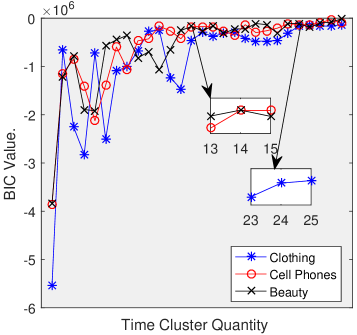
(a) BIC value with the clustering number.

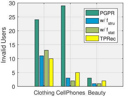
(b) The number of invalid users.

Figure 5. Analyses of different datasets. The left subgraph illustrates how BIC value varies with the clustering number, while the right subgraph illustrates the numbers of invalid users calculated from PGPR and TPRec.

4.1.3. Implementation Details.

To reduce the experiment workload and keep the comparison fair, we closely follow the settings of the PGPR work  (Xian et al., 2019). For the time-aware relation extraction module, we perform relation clustering with GMM and select the optimal number of clusters with Bayesian Information Criterion (BIC)  (Vrieze, 2012). The BIC value with the clustering number is presented in Figure 5a. The optimal clustering numbers are 24, 14, and 14 on Clothing, Cell Phones and Beauty, respectively.

For the time-aware representation learning module, we set the embedding size $d$ as $100$, and the dimension $m$ of temporal feature space as $25$, with 16 dimensions for statistical features and 9 dimensions for structural features. More specifically, for statistical features, we simply compute the $year(t)\in\mathbb{R}^{1}$ to be $=current\ year-earliest\ year$, $day(t)\in\mathbb{R}^{1}=current\ day-earliest\ day$, $month(t)\in\mathbb{R}^{1}$ is the month of the year, $week(t)\in\mathbb{R}^{8}$ is the day in a week and it’s one-hot encoding, and $season(t)\in\mathbb{R}^{5}$ is the season in a year and it’s one-hot encoding. For structural features, given a specific timestamp $t_{1}$, we have $\bm{f}_{stru}(t_{1})\in\mathbb{R}^{9}$ $=z(t_{1})\ ||\ z_{sea}^{\prime}(t_{1})\ ||\ z_{sea}^{\prime\prime}(t_{1})$ $||\ \ z_{mon}^{\prime}(t_{1})\ ||\ z_{mon}^{\prime\prime}(t_{1})$ $||\ z_{week}^{\prime}(t_{1})\ ||\ z_{week}^{\prime\prime}(t_{1})$ $||\ z_{day}^{\prime}(t_{1})\ ||\ z_{day}^{\prime\prime}(t_{1})$.

For the time-aware path reasoning module, we set the maximum episode path length $k$ as $3$ (namely, the maximum history length is $2$), the default history length $k^{\prime}$ as 1, and the maximum size of pruned action space as $|\mathcal{A}_{k}|\leq 250$. Besides, for the parameters in RL, we set the dimension of $x_{t}$ as 256 and the discount factor $\gamma$ as $0.99$; Also, for the policy/value network, we set $W_{1}\in\mathbb{R}^{512\times 256}$ , $W_{a}\in\mathbb{R}^{256\times 251}$ and $W_{c}\in\mathbb{R}^{256\times 1}$. We optimize our model for 50 epochs with Adam, where the learning rate is set as 0.0001 and the batch size is 32. During the prediction, we refer to PGPR (Xian et al., 2019) and set the sampling sizes as $K_{1}=25$, $K_{2}=5$, $K_{3}=1$.

4.1.4. Evaluation Metrics.

We adopt four widely used metrics to evaluate recommendation performance including: Normalized Discounted Cumulative Gain@K (NDCG@K for short), Recall@K, Precision@K and Hit Ratio@K (HR@K for short). The process for obtaining the scores for those metrics is given in Equation (4.1.4).

$$NDCG@K =\frac{DCG@K}{IDCG@K} Recall@K =\frac{\left|TP\right|}{\left|TP\right|+\left|FN\right|}$$

(21) $$Precision@K =\frac{\left|TP\right|}{\left|TP\right|+\left|FP\right|} HR@K =\frac{N_{hits}@K}{N_{users}}$$

Here, DCG@K is the Discounted Cumulative Gain at position K, IDCG@K is Ideal Discounted Cumulative Gain through position K, $\left|TP\right|$ means the number of recommended items that are actually relevant at position K, $\left|TP\right|+\left|FN\right|$ is the total number of relevant items and $\left|TP\right|+\left|FP\right|$ means the number of recommended items at position K. As for HR@K, $N_{hits}@K$ is the number of users whose items in the test set at position K, and $N_{users}$ is the total number of users.

These metrics reflect how a model retrieves relevant items that users are indeed fond of. A larger score indicates the better performance that a model achieves. In our experiments, we refer to  (Xian et al., 2019) and set $\text{K}=10$.

Table 3. Normal test performance comparison on three real-world datasets. The results are reported in percentage (%). The bold font denotes the winner in that column. The row ‘Impv’ indicates the relative performance gain of our TPRec  relative to ADAC.

Models	Clothing				Cell Phones				Beauty
Metrics	NDCG	Recall	HR	Prec.	NDCG	Recall	HR	Prec.	NDCG	Recall	HR	Prec.
BPR	0.598	1.086	1.801	0.196	1.892	3.363	5.323	0.624	2.704	4.927	9.113	1.066
RippleNet	0.627	1.112	1.885	0.201	1.935	3.858	5.727	0.688	2.458	5.251	9.224	1.133
TransRec	1.245	2.078	3.116	0.312	3.361	6.279	8.725	0.962	3.218	4.853	8.671	1.285
PGPR	2.871	4.827	7.023	0.723	5.042	8.416	11.904	1.274	5.573	8.476	14.682	1.744
ADAC	3.048	5.027	7.502	0.763	5.220	8.943	12.537	1.358	6.080	9.424	16.036	1.991
w/ $\bm{f_{stru}}$	3.074	5.132	7.484	0.778	5.988	10.185	14.278	1.528	6.185	9.582	16.130	2.023
w/ $\bm{f_{stat}}$	2.997	5.144	7.498	0.781	5.743	9.714	13.649	1.471	5.868	9.227	15.719	1.928
TPRec	3.109	5.298	7.657	0.798	5.643	9.572	13.553	1.463	5.963	9.184	15.678	1.919
Impv.(%)	+2.01	+5.39	+2.07	+4.59	+14.71	+13.89	+13.89	+12.52	+1.73	+1.68	+0.59	+1.66

Table 4. Sequence-based performance comparison. The results are reported in percentage (%).

Models	Side Infomation		Clothing		Cell Phones		Beauty
	KG?	Time?	NDCG	Recall	NDCG	Recall	NDCG	Recall
BERT4Rec	$\times$	✓	0.248	0.516	1.612	3.315	1.664	3.540
GRU4Rec	$\times$	✓	0.541	1.070	3.370	6.365	3.813	6.508
NextItNet	$\times$	✓	0.289	0.573	2.422	4.683	2.360	4.727
SR-GNN	$\times$	✓	0.428	0.797	3.072	5.777	3.212	5.757
GC-SAN	$\times$	✓	1.116	2.229	4.211	8.219	4.361	7.511
SASRec	$\times$	✓	1.253	2.541	3.876	7.695	4.522	8.918
TimelyRec	$\times$	✓	1.263	2.716	4.039	7.791	4.671	9.217
PGPR	✓	$\times$	2.102	3.651	3.135	4.911	3.654	6.060
w/ $\bm{f_{stru}}$	✓	✓	2.245	3.905	4.228	8.936	4.331	8.051
w/ $\bm{f_{stat}}$	✓	✓	2.270	3.955	4.123	8.767	4.175	7.717
TPRec	✓	✓	2.304	4.027	4.292	9.131	4.467	8.773

4.2. Performance Comparison (RQ1)

Table 3 presents the performance of the compared normal test methods in terms of four evaluation metrics. For the sake of clarity, the row ‘Impv’ shows the relative improvement achieved by our TPRec or w/ $\bm{f_{stru}}$ over the best baselines. Table 4 presents the sequence-based recommendation methods performance comparison. The boldface font denotes the winner in that column. We make the following observations:

4.2.1. TPRec  Vs. existing normal test methods.

From Table 3, we observe our TPRec  always achieve the best performance among all compared methods. Especially in the dataset Cell Phones, the improvement of w/ $\bm{f_{stru}}$ over best baselines are quite impressive — 14.71%, 13.89%, 13.89%, and 12.52% in terms of NDCG, Recall, HR, and Precision, respectively. And our TPRec  performs significantly better ($p$-value < 0.05) than those open source baselines (PGPR, TransRec, etc.) with three repeated trials. This result validates that by leveraging temporal information our TPRec  is able to find higher-quality reasoning paths.

We make a further investigation to provide more insights. We refer to a path as an invalid path if the path starts from a user but doesn’t end at an item entity within three hops (note that we set the path length $k=3$). We also refer to a target user that we predict as an invalid user if he has less than 10 valid paths. As shown in Figure 5b, we find the number of Invalid Users in TPRec is consistently less than PGPR which does not consider temporal information. This result suggests that time-aware rewards adopted by TPRec indeed guide the RL agent towards exploration better.

4.2.2. Comparison in terms of different datasets.

Interestingly, in normal test setting, we observe that the improvement of our TPRec over recent work on the datasets Clothing and Cell Phones are relatively large, while relatively small on the dataset Beauty. This result can be explained by the difficulty of different datasets. From Figure 5b, we observe that the number of invalid users on the Beauty dataset generated by PGPR is $3$, while the number increases to $24$ and $29$ on other datasets. This result validates that path reasoning on Beauty is relatively easier than on other datasets. PGPR or ADAC also achieve pretty good performance on Beauty. Correspondingly, our TPRec does not obtain much gain on Beauty.

4.2.3. Reasoning Vs. Unreasoning.

We also observe that KG-based reasoning methods (i.e., PGPR, ADAC and TPRec) outperform other KG-based methods (i.e., RippleNet) on all three datasets across all four evaluation metrics. This result clearly validates the superiority of conducting path reasoning on knowledge graph. Though reasoning, interpretability is not against accuracy. It not only increases interpretability, but also boosts model accuracy.

4.2.4. TPRec  Vs. existing sequence-based methods.

From Table 4, we can see the performance of TPRec and PGPR is lower than that at normal test setting. One possible reason of the performance drop is the Out-of-Distribution (OOD) setting in the sequence-based experiment, which means the test distribution is different from the training. Our TPRec achieves the best performance on the Clothing and the Cell Phones datasets, whereas, slightly worse than TimelyRec and SASRec on the Beauty dataset. It is appropriate to emphasize that these sequential recommendation methods are specifically designed for predicting the next item that the user would interact, which sacrifices explainability. Our TPRec can not only provide explanations about why an item is suitable for a user, but also achieve comparable recommendation accuracy in sequential recommendation.

We further make the following observations. In the Clothing dataset, even PGPR is much better than other sequence-based methods, which indicates that the KG side information is really useful in the Clothing dataset. Additionally, our TPRec consistently beats PGPR in all datasets, and TPRec performs better than the other two versions, $w/f_{stru}$ and $w/f_{stat}$. Notably, there is 10% of the interactions in validation set between training set and test set in sequence-based comparison, and the time-series clustering method doesn’t know the interaction distribution around the test set, which is different from normal test setting. Hence, $w/f_{stru}$’s effect is not enough to support such experiments, it needs to be supplemented by $w/f_{stat}$. This verifies the validity of our time-aware reasoning methodology.

Table 5. Characteristics and performance of TPRec and its variants in normal test setting. The ‘Imp(%).’ is relative to TPRec.

Methods	Reasoning With.		Equipped with.		Performance
	Time-aware	BLSTM	Statistical	Structural	Clothing		Cell Phones		Beauty
	Reward?	Encoder?	Feature?	Feature?	Prec.	Recall	Prec.	Recall	Prec.	Recall
PGPR	$\times$	$\times$	$\times$	$\times$	0.723	4.827	1.274	8.416	1.744	8.476
Imp(%)					-9.40	-8.89	-12.9	-12.1	-9.12	-7.71
w/o R	$\times$	✓	✓	✓	0.191	1.374	0.317	1.909	0.712	3.031
Imp(%)					-76.1	-74.1	-78.3	-80.1	-62.9	-67.0
w/o L	✓	$\times$	✓	✓	0.786	5.205	1.450	9.534	1.927	9.200
Imp(%)					-1.50	-1.76	-0.89	-0.40	+0.42	+0.17
w/ $\bm{f_{stru}}$	✓	✓	$\times$	✓	0.778	5.132	1.528	10.185	2.023	9.582
Imp(%)					-2.51	-3.13	+4.44	+6.40	+5.42	+4.33
w/ $\bm{f_{stat}}$	✓	✓	✓	$\times$	0.781	5.144	1.471	9.714	1.928	9.227
Imp(%)					-2.13	-2.91	+0.55	+1.48	+0.47	+0.47
TPRec	✓	✓	✓	✓	0.798	5.298	1.463	9.572	1.919	9.184

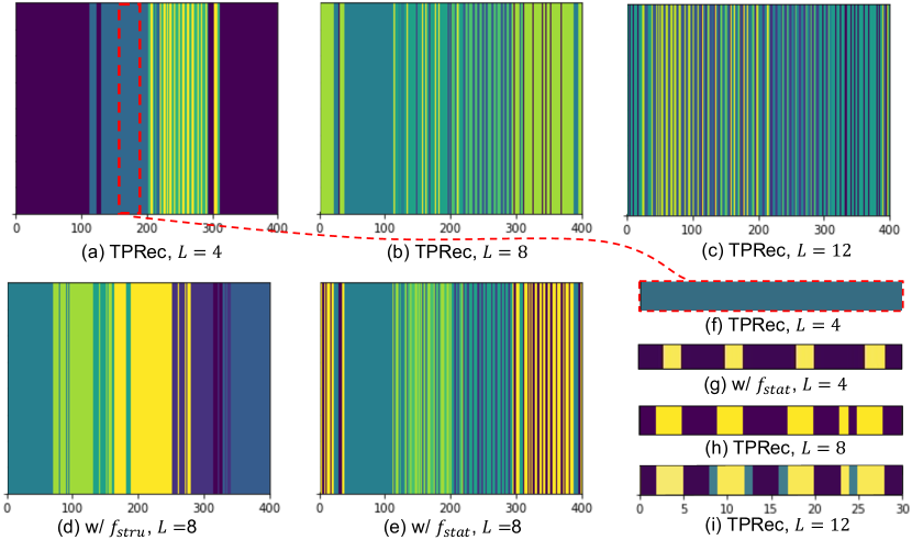
Figure 6. Visualization of the clustering of the relations with varying timestamp on the Cell Phones dataset. The color represents the class that the timestamp belongs to.

4.3. Ablation Study (RQ2)

Note that TPRec improves PGPR mainly in the following three aspects: using temporal features to extract relations, adopting personalized time-aware reward strategy, and using bidirectional LSTM to encode the state vector. To show the impact of these aspects, besides making a comparison among three versions of TPRec (w/ $\bm{f_{stru}}$, w/ $\bm{f_{stat}}$ and TPRec), we further conduct ablation studies and compare TPRec with its two variants: (1) w/o R that removes personalized time-aware weighting strategy $W_{h_{u}}$ in generating rewards and uses average pooling instead. (2) w/o L that replaces bidirectional LSTM with a simple fully connected layer as PGPR. The characteristics and performance of these methods are presented in Table 5.

4.3.1. Effectiveness of using temporal features.

First, we observe our TPRec(i.e., w/ $\bm{f_{stru}}$, w/ $\bm{f_{stat}}$ and TPRec) that use temporal features consistently outperform PGPR. This result validates the essence of temporal information in making recommendation. We then make a comparison among three versions of TPRec. To our surprising, w/ $\bm{f_{stru}}$ that just uses structure features usually achieves better performance than TPRec which uses both statistical and structural features in normal test setting. To gain more insights of this phenomenon, we visualize the results of the Cell Phones dataset clustering in Figure 6, and the other two datasets have similar performance. We observe that with the cluster number $L$ gaining, the clustering result in TPRec turns to be more complicated. For example, in Figure 6a, the clustering result of TPRec is similar with the four seasons in one year, and then we focus on 30 days in the second season (Figure 6f). As the $L$ grew to $8$, it broke the seasons’ pattern, and could obtain weekend-like clusters (Figure 6h). It’s worth noting that w/ $\bm{f_{stat}}$ (Figure 6g) also distinguishes between weekdays and weekends, but our TPRec clustering is more flexible, which benefits from the structural features. When $L=12$ in Figures 6c and 6i, the clusters become even more precise. Furthermore, in Figure 6b, 6d and 6e, we can see that the clustering is more stable in w/ $\bm{f_{stru}}$, where the interactions with similar tendencies are more likely to be clustered into the same class, while we observe relatively heavy fluctuation in w/ $\bm{f_{stat}}$. This interesting phenomenon suggests that the structural features deduced from user behaviors provide an important and reliable signal in capturing interaction similarity, while statistical features exhibit weak or even noisy correlation with the similarity. Nonetheless, the statistical features sometimes are also useful and serve as a complement for relation extraction. It can be seen from the better performance of TPRec over w/ $\bm{f_{stru}}$ on dataset Clothing and all three datasets in sequence-based test setting.

4.3.2. Effectiveness of using time-aware reward.

From Table 5, when removing personalized time-aware weighting strategy in reward, we observe significant performance degradation (higher than 69.21%) of w/o R compared with TPRec. w/o R even performs worse than PGPR. This interesting phenomenon clearly reveals the importance of using personalized weights. Time-aware relations are indeed useful for path reasoning, but they require to be carefully exploited. Only if we finely differentiate the contribution of each type of relation, can we sufficiently enjoy the merits of such information.

4.3.3. Effectiveness of using bidirectional LSTM

By comparing w/o L with TPRec, generally speaking, we can conclude that using bidirectional LSTM could boost recommendation performance. This result can be attributed to the powerful capacity of BLSTM in capturing dependency between reasoning hops. However, on the dataset Beauty, TPRec performs closely or even worse than w/o L. This phenomenon can be attributed to the specialty of Beauty. As discussed in Section 4.2, Beauty is a relatively simple dataset and does not need such complex structure. The advanced BLSTM may not bring much gain on Beauty and instead would increase the risk of over-fitting.

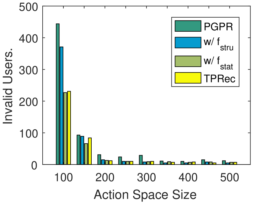
(a) Clothing.

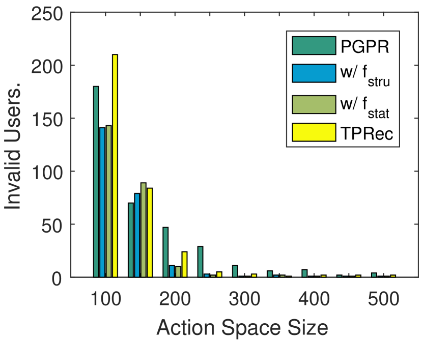
(b) Cell Phone.

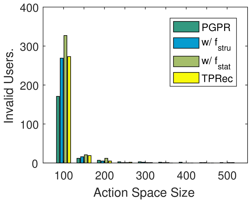
(c) Beauty.

Figure 7. Invalid User number of varying action space size $\epsilon$.

4.4. Parameter Study on Path Reasoning Module. (RQ3)

To provide more insights on the time-aware path reasoning module, we test the performance of TPRec with different time cluster quantity, action space size $\epsilon$ and state history length $k^{\prime}$.

4.4.1. Effect of Time Cluster Quantity.

Figure 8 presents the performance of four compared methods with different time cluster $L$ in range {4, 8, 12, 16, 20, 24 }. We make the following three observations: (1) With few exceptions, our TPRec consistently outperforms PGPR in all three datasets. (2) In the Cell Phones and Beauty dataset, all three versions of TPRec perform better when the number of time cluster $L=12$ or $16$. And when $L$ is too small or too large, the performance of all three methods drops slightly. (3) In the Cloth dataset, when $L$ increases, the performance of our methods is relatively stable. This is consistent with our strategy to adaptively determine time cluster number by BIC value (in Section 4.1.3), and shows that BIC value can provide a suitable reference for clustering number $L$.

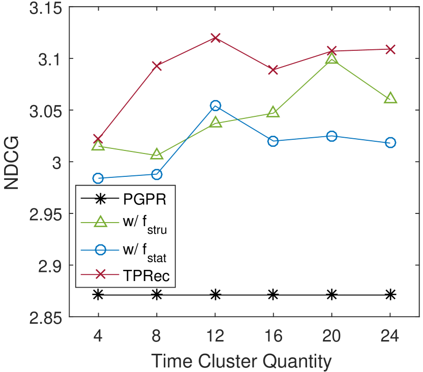
(a) NDCG (Clothing).

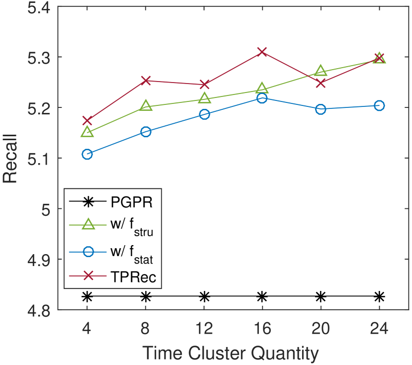
(b) Recall (Clothing).

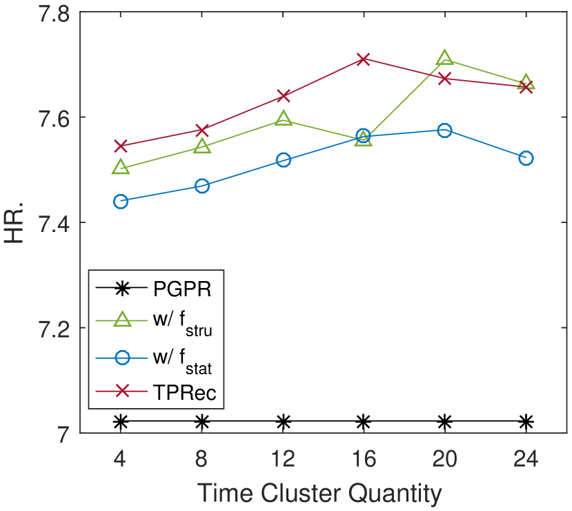
(c) HR (Clothing).

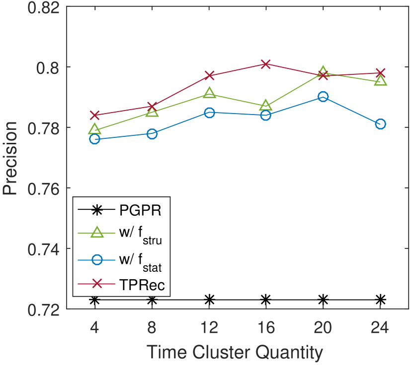
(d) Precision (Clothing).

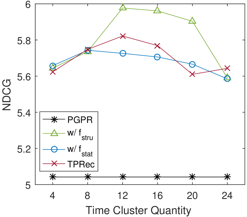
(e) NDCG (Clothing).

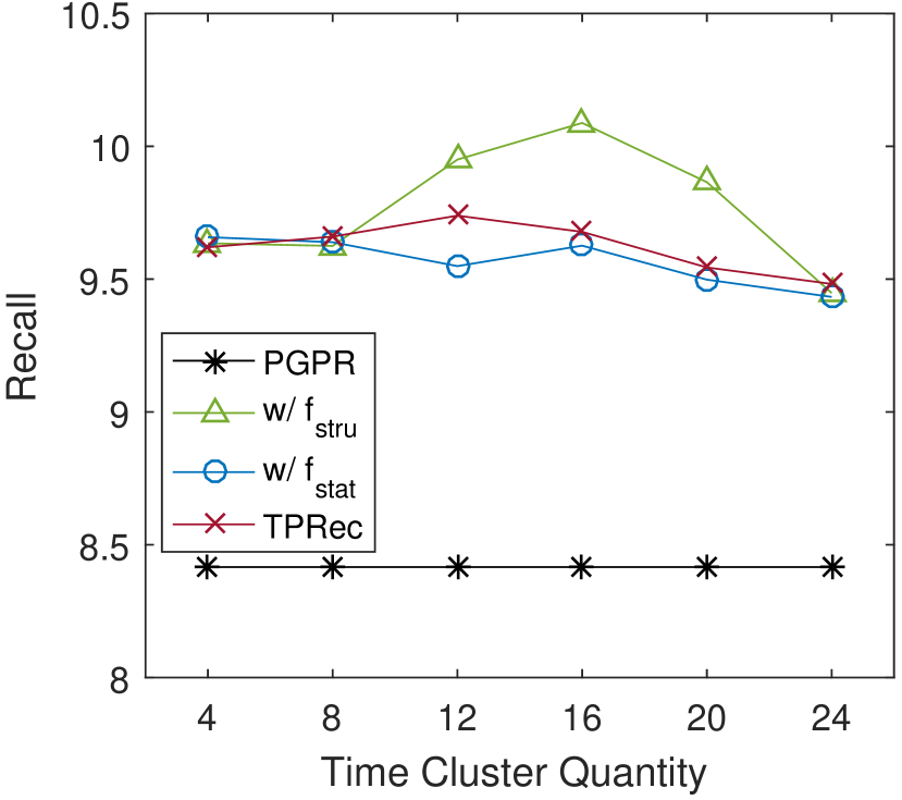
(f) Recall (Cell).

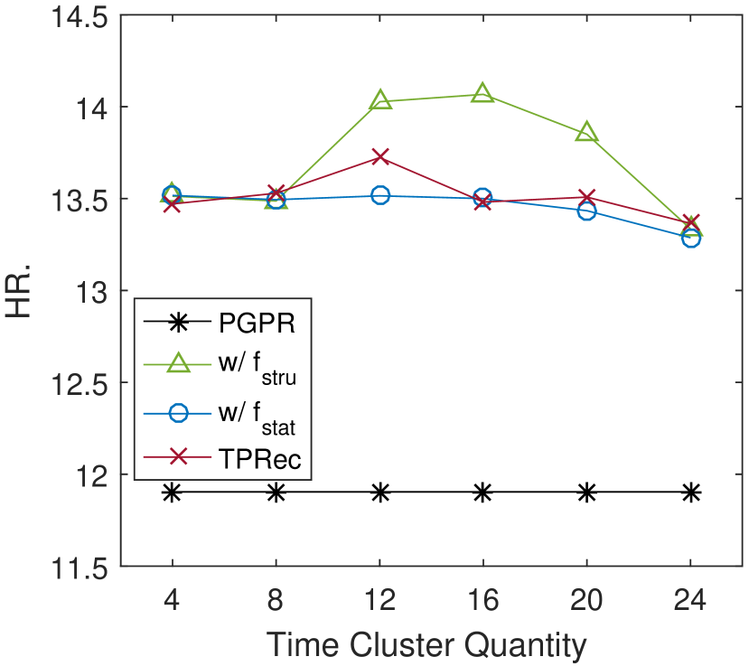
(g) HR (Cell).

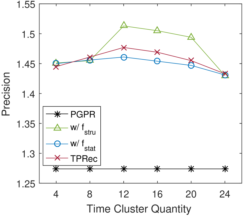
(h) Precision (Cell).

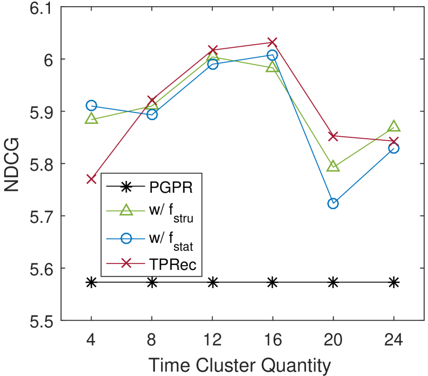
(i) NDCG (Beauty).

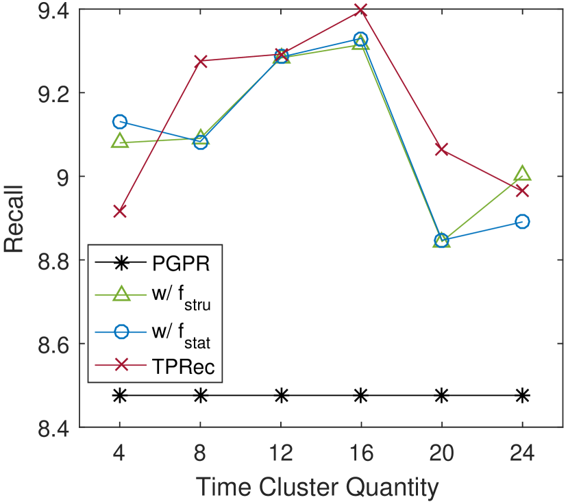
(j) Recall (Beauty).

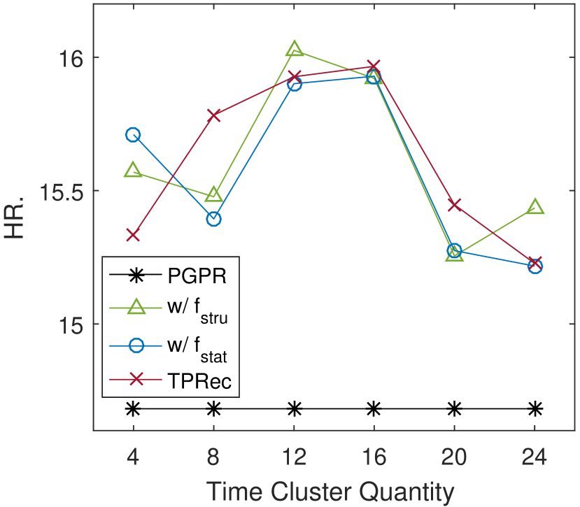
(k) HR (Beauty).

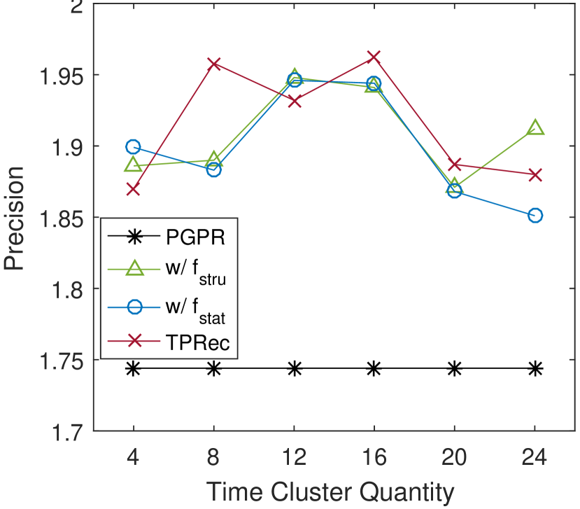
(l) Precision (Beauty).

Figure 8. Effect of varying time cluster quantity $L$.

4.4.2. Effect of Action Space Size.

Figure 9 presents the performance of four compared methods with different action space size $\epsilon$ varying from 100 to 500. We make the following two observations: (1) With few exceptions, all three versions of TPRec consistently outperform PGPR with various $\epsilon$, demonstrating the effectiveness of exploiting temporal information. (2) As the action space size $\epsilon$ increases, generally speaking, the performance will become better at the beginning. The reason is that when the action space size $\epsilon$ is too small, the model is likely to miss the relevant paths. It also can be seen from Figure 7, that a smaller action space size (e.g. $\epsilon\leq 200$) would incur a larger number of invalid users. (3) But when the $\epsilon$ surpasses a certain threshold, the performance of all the methods drops with $\epsilon$ further increasing. The reason is that a larger action space would increase the risk of retrieving irrelevant paths. Nonetheless, our TPRec drops relatively mildly. It demonstrates our TPRec is more robust to $\epsilon$ and able to identify high-quality paths by leveraging temporal information.

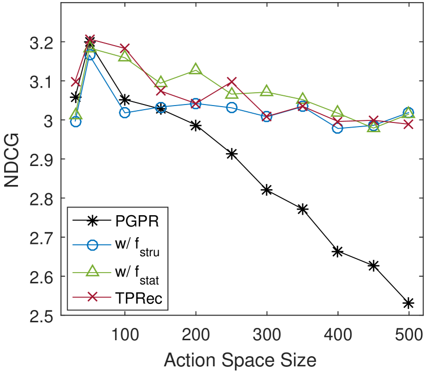
(a) NDCG (Clothing).

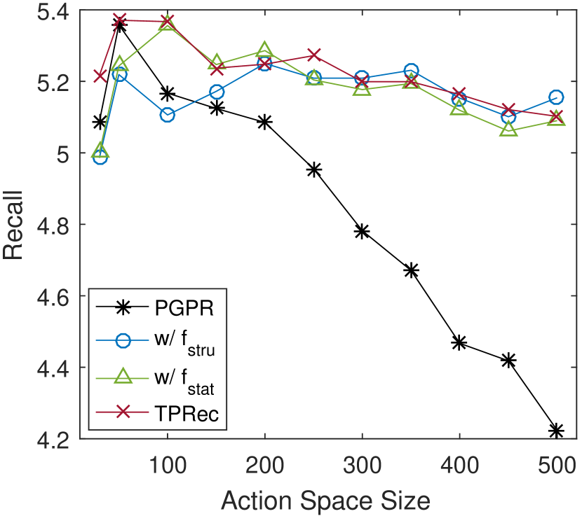
(b) Recall (Clothing).

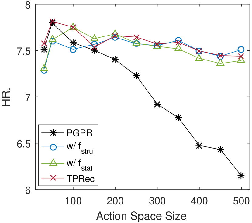
(c) HR (Clothing).

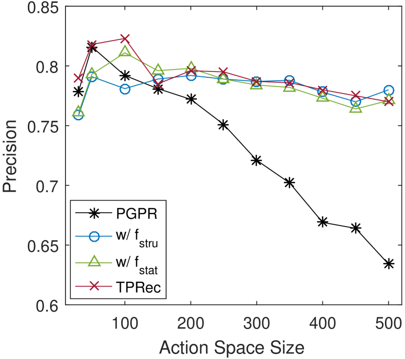
(d) Precision (Clothing).

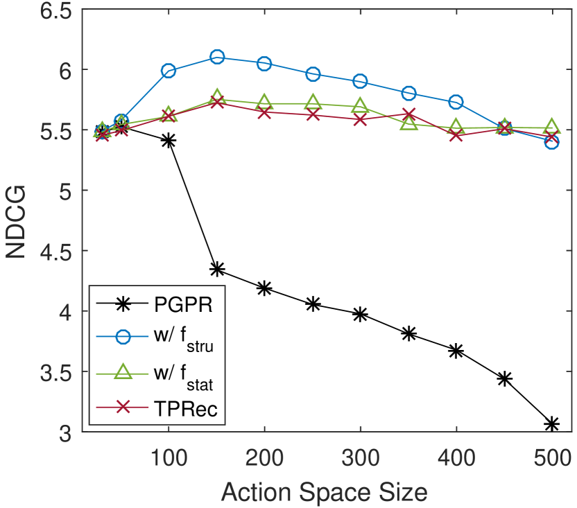
(e) NDCG (Cell).

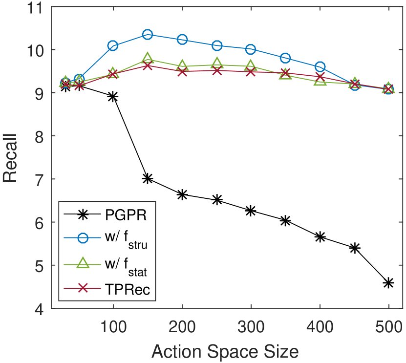
(f) Recall (Cell).

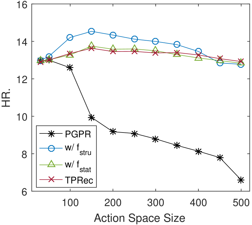
(g) HR (Cell).

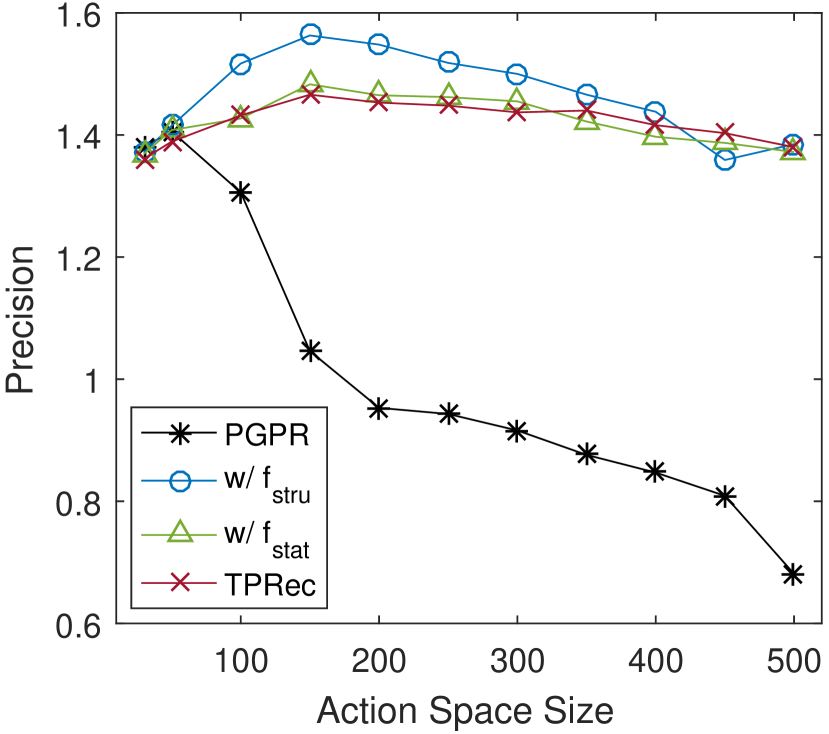
(h) Precision (Cell).

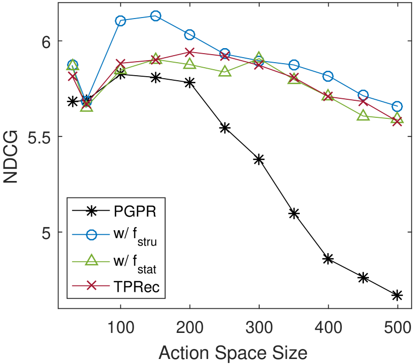
(i) NDCG (Beauty).

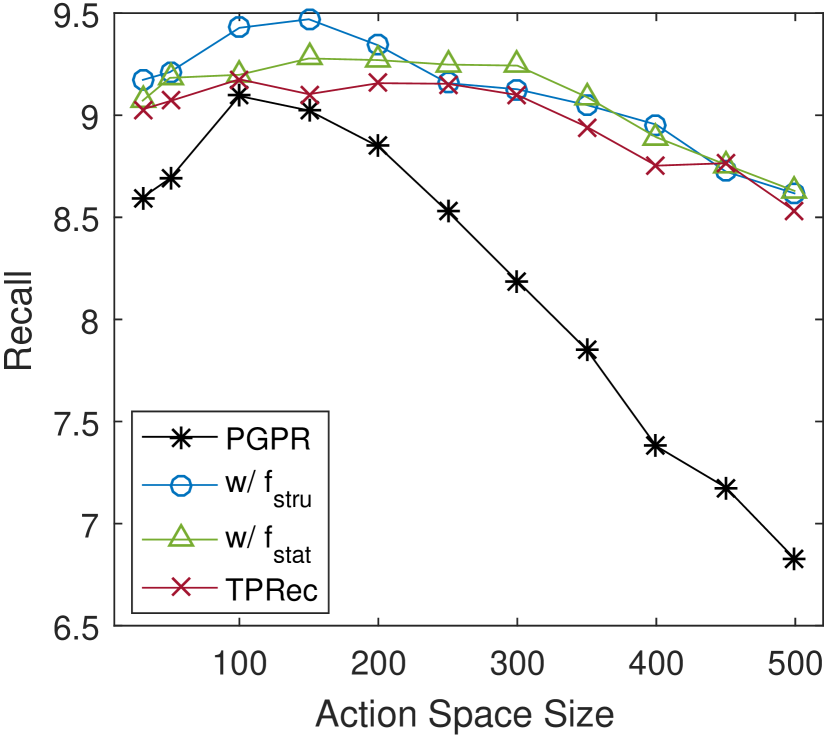
(j) Recall (Beauty).

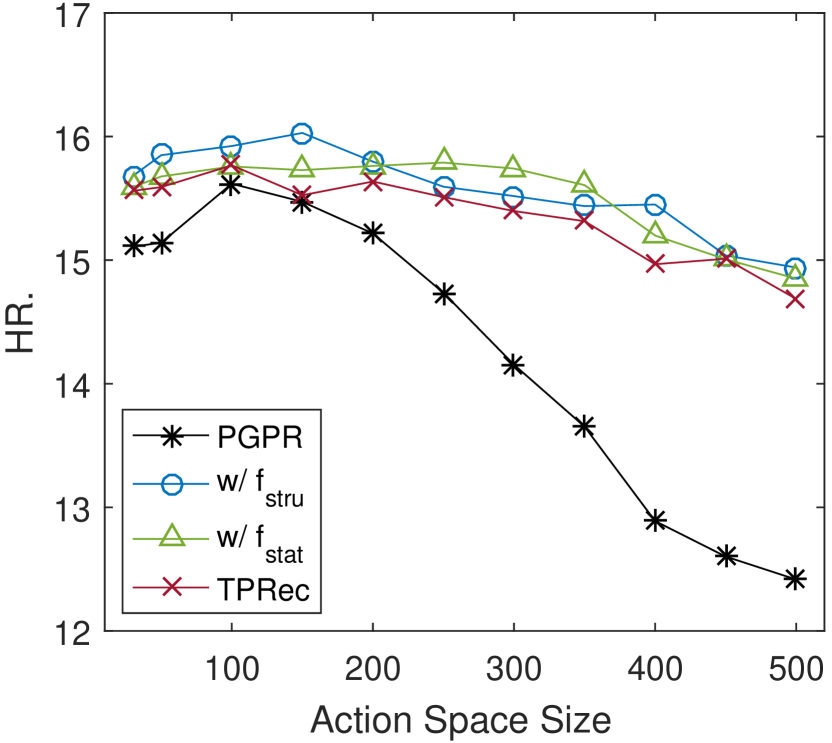
(k) HR (Beauty).

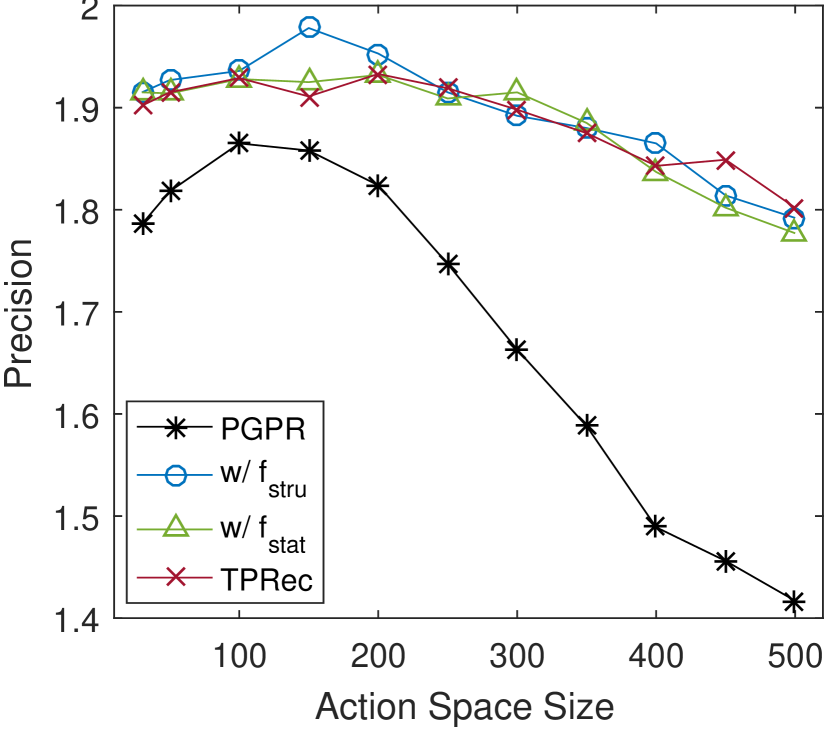
(l) Precision (Beauty).

Figure 9. Effect of varying action space size $\epsilon$.

4.4.3. Effect of State History Length.

Figure 10 presents the performance of four compared methods with different State History Length $k^{\prime}$ in range $\{0,1,2\}$. We make the following observations: (1) with few exceptions, our TPRec consistently outperforms PGPR. (2) For all methods, the versions with encoding 1-step or 2-step history consistently outperform those without encoding history. This result validates the effectiveness of exploiting historical states to learn policy. But, we observe that encoding 2-step history may not be superior over 1-step. Too long history will bring some irrelevant information or even noises, which deteriorates recommendation performance.

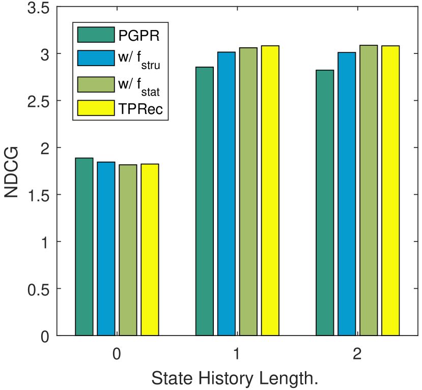
(a) NDCG (Clothing).

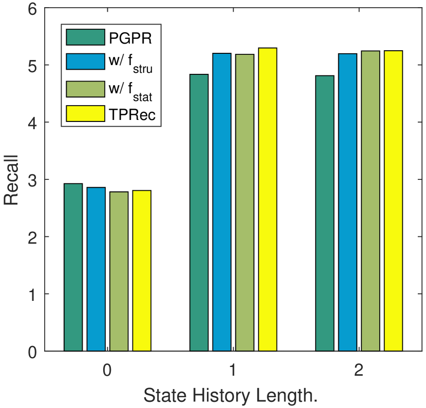
(b) Recall (Clothing).

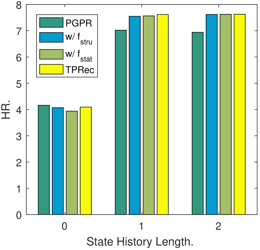
(c) HR (Clothing).

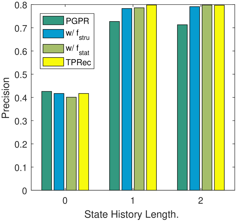
(d) Precision (Clothing).

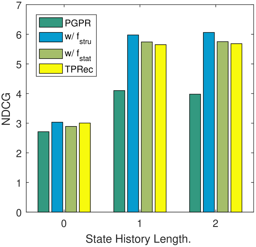
(e) NDCG (Clothing).

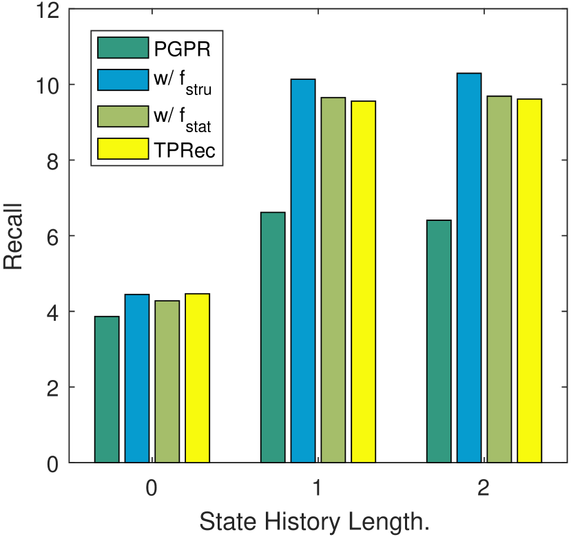
(f) Recall (Cell).

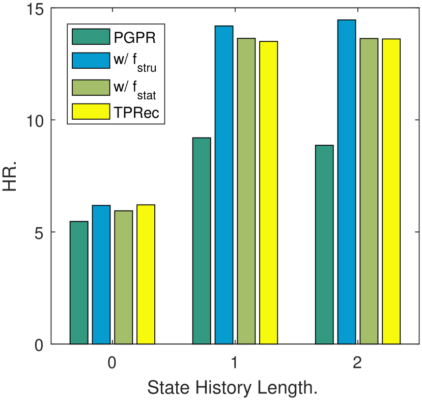
(g) HR (Cell).

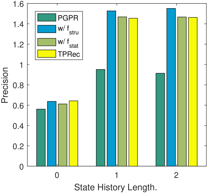
(h) Precision (Cell).

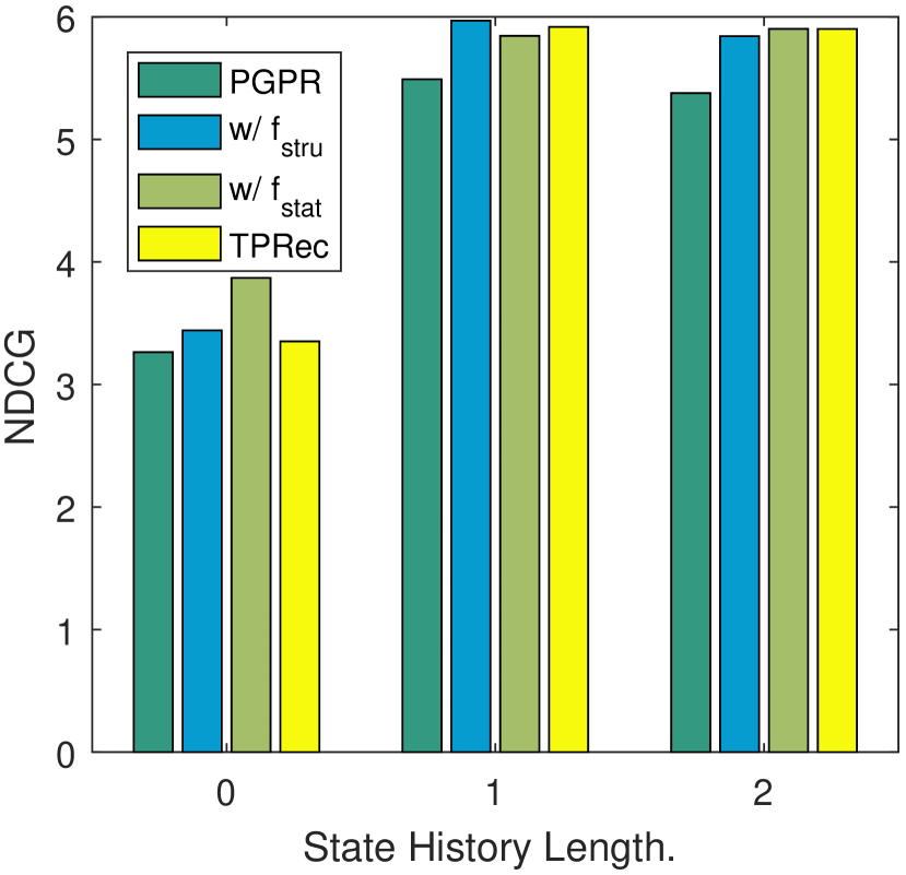
(i) NDCG (Beauty).

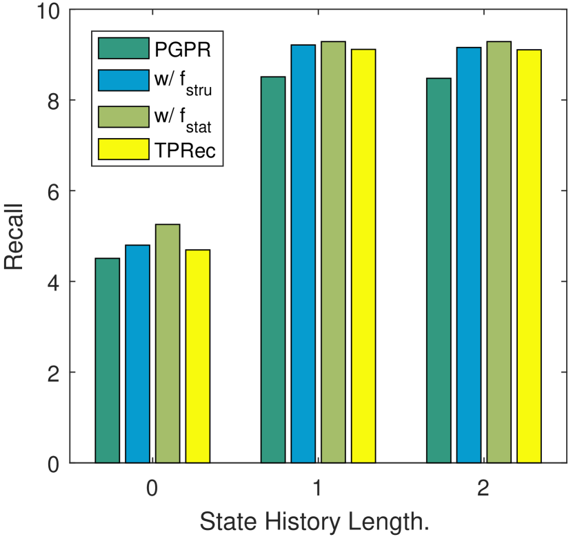
(j) Recall (Beauty).

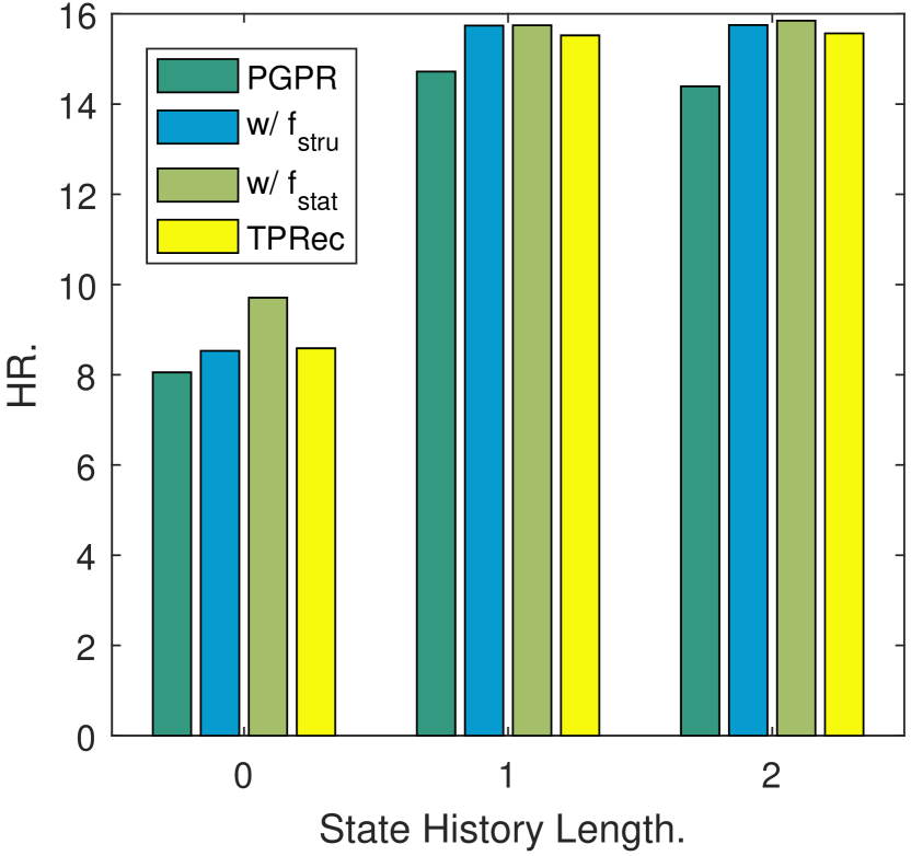
(k) HR (Beauty).

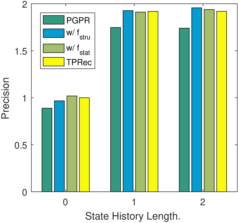
(l) Precision (Beauty).

Figure 10. Effect of varying state history length $k^{\prime}$.

4.5. Evaluating Explanations (RQ4)

How to evaluate explanations in recommender system is a hard problem. Fortunately, inspired by (Tan et al., 2021; Zhao et al., 2020), we mathematically define a user-oriented evaluation metric to evaluate explainability. And finally, we give a case study to demonstrate explanations.

4.5.1. Explainability Evaluation

To automatically evaluate the quality of explanations generated by TPRec, we adopt the user’s reviews on items as the ground truth reason about why the user purchased the item, as previous works(Tan et al., 2021; Zhao et al., 2020; Chen et al., 2019, 2018b; Li et al., 2020b; Wang et al., 2018a; Wu et al., 2022; Wang et al., 2021b; Li et al., 2022) do. Here, for reasoning paths $\tau_{u,\hat{V}}$ that an item $\hat{v}\in\hat{V}$ recommended to user $u$ before position $K$, we extract all the Word feature entities as an explanation list, which is defined as $S_{u}=[s^{(0)}_{u},s^{(1)}_{u},...,s^{(r)}_{u}]$. Thus, if a reasoning path contains more entities that are mentioned in ground truth reviews, it will achieve better explainability. More specifically, we filter less salient review words if their frequency is more than 5000 and TF-IDF ¡ 0.1, and the remaining words are our ground truth reason $G_{u}=[g^{(0)}_{u},g^{(1)}_{u},...,g^{(n)}_{u}]$.

Then for each user, we calculate the $Recall$, $Precision$ and $F_{1}$ score of the reasoning path’s $Word$ entities $S_{u}$ with regard to the ground truth $G_{u}$:

(22) $$Recall =\frac{|S_{u}\cap G_{u}|}{|G_{u}|+1}, Precision =\frac{|S_{u}\cap G_{u}|}{|S_{u}|+1}, F_{1} =2\cdot\frac{Precision\cdot Recall}{Precision+Recall+1},$$

where $Recall$ measures the percentage of aspects liked by the user included in our explanation, $Precision$ indicates how much our explanation is liked by the user, and $F_{1}$ score is the harmonic mean between those two. And the $+1$ in the denominator is used to avoid dividing by $0$. Finally, we average the scores of all users to evaluate explainability.

Table 6. Explanation performance comparison between PGPR and TPRec on different datasets.

Dataset	Cloth			Cellphone			Beauty
Metric	Recall	Prec.	F1	Recall	Prec.	F1	Recall	Prec.	F1
PGPR	23.771	90.750	19.340	22.970	90.623	18.522	19.296	90.879	15.936
TPRec	24.642	90.871	21.133	23.637	90.895	19.043	20.093	90.891	17.471

From Table 6, our TPRec outperforms PGPR in all three datasets. Though not strictly, it provides an angle to show that the use of temporal information can achieve better explainability.

4.5.2. Case Study

To better understand how temporal information boosts the quality of explainable recommendation, we conduct a case study based on the result of our TPRec. As shown in Figure 11, we provide several examples of the learned reasoning paths with hop scores, where the path marked in red denotes the top relevant one predicted by TPRec.

The first example (Case 1) comes from the Clothing dataset, where we make a recommendation for a specific user on 24-11-2013. By leveraging temporal information, our TPRec  can deduce the weather is winter and correspondingly identify the most relevant word is “cold”. Based on such knowledge, TPRec  is able to retrieve more relevant “sweater” to the user, while PGPR that does not use temporal information would fall short. In the second example (Case 2), there are two users who both bought an “iPhone” on 24-3-2014 and 12-1-2014 respectively. The second user also purchased a ”phone” on 05-8-2013 and a ”charger line” on 11-2-2014. As we can see, our TPRec  recommends “charge line” instead of “phone” as it could capture the common sense that a person is unlikely to buy two mobile phones in a short time. The last example (Case 3) depicts two reasoning paths of a user purchasing ”shampoo”. Our TPRec  could differentiate the better one — the red path is more reasonable, as the link “purchase” happened on the day 4-7-2013, which is the shopping festival as the day 11-11-2013. Naturally, the user on 11-11-2013 is more likely to have similar needs as on 4-7-2013, and the item from the red path is more likely to be favored by the user.

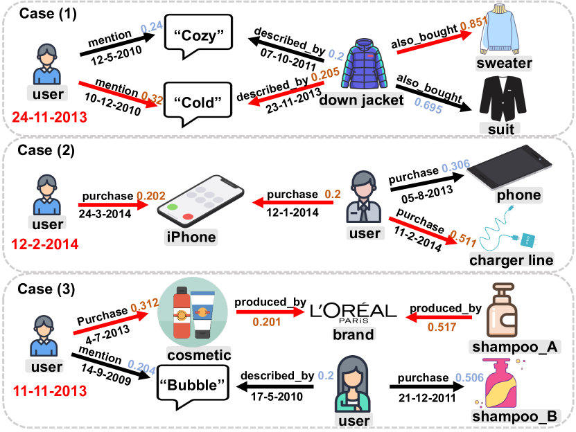
Figure 11. Case study on how temporal information benefits explainable recommendation. The timestamp in red font below “user” depicts the recommended date. The path marked in red denotes the top relevant one predicted by TPRec.

5. Related Work

We divide the related works into three categories: (i) knowledge graph based recommendation, (ii) temporal knowledge graph embedding and (iii) temporal information in recommendation.

5.1. Knowledge Graph Based Recommendation

Existing studies on KG-based recommendation systems (Guo et al., 2020) can be roughly grouped into two sub-categories: embedding-based methods and path-based methods.

Embedding-based methods adopt a common general model, where the latent vector $\bm{u}_{i}$ of each user $u_{i}$ and item embedding $\bm{v}_{j}$ can be extracted from KGE, and the probability of item $v_{j}$ being recommended to user $u_{i}$ can be calculated by $\hat{y}_{i,j}=f\left(\mathbf{u}_{i},\mathbf{v}_{j}\right)$. Note that $f(\cdot)$ can be either DNN, inner product, or other scoring functions. For instance, (Zhang et al., 2016) proposed CKE, which uses TransE to unify the KG information in the CF framework. Deep Knowledge-based Network (DKN) (Wang et al., 2018d) treats entity embeddings and word embeddings as different channels, where Kim CNN (Kim, 2014) is used to combine them together for news recommendation. (Huang et al., 2018) uses a GRU network with a knowledge-enhanced key-value memory network, named KSR, to capture user preferences from the sequential interactions. (Wang et al., 2019a) and (Wang et al., 2021a) employ the message passing mechanism of graph neural networks over KG to model the higher-order connections among users, entities, and items.

In the line of path-based methods, recommendations are made based on the connectivity patterns of the entity in user-item graph. For example, (Hu et al., 2018) uses CNN to obtain each path instance’s embedding. (Wang et al., 2019c) proposed a knowledge-aware path recurrent network (KPRN) solution, which constructs the extracted path sequence with both the entity embedding and the relation embedding, and encodes the path sequence with an LSTM layer before recommendation. RippleNet (Wang et al., 2018c) combined embedding-based and path-based methods and modeled users’ preference propagation by their historical interests along the path in the KG. Inspired by KG reasoning techniques (Xiong et al., 2017; Lin et al., 2018; Das et al., 2017), PGPR (Xian et al., 2019) performs reinforcement policy-guided path reasoning over KG-based user-item interaction. Inspired by such RL-based policy networks, CPR (Lei et al., 2020) models conversational recommendation as a path reasoning problem on a heterogeneous graph. Different from PGPR which relies on sparse reward signal, ADAC (Zhao et al., 2020) adopts an Adversarial Actor-Critic model to achieve faster converge.

These KG reasoning methods (e.g., (Xian et al., 2019; Zhao et al., 2020; Lei et al., 2020)) can provide explainable reasoning paths while obtaining accurate recommendation results. However, they do not use temporal information and may lead to inappropriate recommendations. Therefore, we propose TPRec, aiming to leverage temporal information for promoting explainable recommendation.

5.2. Temporal Knowledge Graph Embedding

Existing studies on knowledge graph embedding research focus on static knowledge graphs. A series of these models are variations of TransE (Bordes et al., 2013; Ji et al., 2015; Wang et al., 2014; Lin et al., 2015). These models assume that facts are not changing with time, which is obviously contrary to reality. Therefore, recent studies begin to take temporal information (e.g., fact occurrence time, end time, etc.) into consideration (Ji et al., 2020), which turns out to further improve the performance of KG embedding.

There exist only a few studies on temporal knowledge graph (TKG) embedding. (Leblay and Chekol, 2018) proposed TTransE by simply extending existing embedding methods like TransE. TTransE adopts translational distance score functions to learn associations between facts of a KG. (Ma et al., 2019) generalized existing models for static knowledge graphs to temporal knowledge graphs with a timestamp embedding. (Dasgupta et al., 2018) took a timestamp as a hyper-plane and projected entities and relations to learn KG embedding.

TKG embedding has to deal with two types of dynamics, namely, entity dynamics and relation dynamics.

Entity dynamics refers to the fact that real-world events can change the state of a given entity’s state and therefore affect its corresponding relations. (Trivedi et al., 2017) modeled the occurrence of a fact as a temporal point process, and used a novel recurrent network to learn the representation of non-linearly evolving entities. (Wijaya et al., 2014) formulated the temporal scoping problem as a state change detection problem and utilized the context to learn the states and the state change vectors.

Relation dynamics refers to the fact that the relations among entities in a knowledge graph may change over time. (Jiang et al., 2016) realized that there exist temporal dependencies in relational chains following the timeline, for example, $(P,\text{wasBornIn},\_)$ $\rightarrow$ $(P,$ graduateFrom , $\_)$ $\rightarrow$ $(P,\text{workAt},\_)$ $\rightarrow$ $(P,\text{diedIn},\_)$, and found that many facts are only valid during a short time period. To solve that issue, the authors proposed two time-aware KG completion models to incorporate the above two kinds of temporal information.

Although those TKG embedding methods achieve better performance than traditional KG embedding methods, none of them have considered if only part of the facts is updated very frequently, which is common in recommendation and dealed by our TPRec.

5.3. Temporal Information in Recommendation

Temporal Information is important contextual information for providing users with an accurate prediction based on historical behaviors(Campos et al., 2014). (Yi et al., 2014) finds that dwell time is an important factor to quantify how likely an item is relevant to a user. (Liang et al., 2012) uses the temporal information in micro-blogs in order to profile users’ time-sensitive topic interests. (Chang et al., 2017) proposes sREC, which captures temporal dynamics of users and topics under steaming settings, to perform real-time recommendations. (Hansen et al., 2020) proposes CoSeRNN and leverages time context and device context for better music recommendation. As for temporal patterns of user behaviors, (Ye et al., 2020) and (Li et al., 2020a) discover “absolute” and “relative” time patterns and jointly learn those temporal patterns to model user dynamic preferences and predict future items. (Cho et al., 2021) defines the periodic and evolving patterns of user preferences, and proposes a cascade of two encoders with an attention module to capture such temporal patterns.

Recently, KG-based methods achieve great success for many temporal tasks. (Wang et al., 2020) uses both sequence- and knowledge-level state representations to capture user preference with an induction network, and adopt a composite reward to capture both sequence-level and knowledge-level information for sequential recommendation. (Huang et al., 2018) uses GRU to capture the user’s sequential preference, and utilizes knowledge base information to model the user’s attribute-level preference. (Huang et al., 2019) designs EIUM, which represents KG with multi-modal fusion, and adopts a masked self-attention model to encode the user’s sequential interactions for capturing her dynamic interests. Most of those methods with temporal information consider KG information as enhanced representation to assist sequential recommendation. Our work differs from these works by modeling the statistical and structural temporal patterns between user-item interactions to construct TCKG, and propose time-aware path reasoning over the TCKG to make full use of the structural constraints in KG. It’s inconvenient to utilize our TPRec to predict the next item task like other sequential recommendation methods, because the KG data is different from the sequence data. That is, we need to construct a dynamic edge MASK matrix on KG’s adjacency matrix to avoid the next item $v$’s information and other items behind $v$ from influencing the training phase. We will leave this as our future work.

6. Conclusion

In this paper, we present TPRec, a novel time-aware path reasoning model for recommendation, which addresses the timeliness of interpretation. To the best of our knowledge, the TPRec method is the first work to introduce time-aware path reasoning method into a recommendation system and achieves significant performance improvement by leveraging the temporal information.

Our model first uses time-aware interaction relation extraction component to construct TCKGs for the reasoning environment. Then the time-aware representation learning component encodes entities and relations to get proper representation. Finally is the key time-aware reasoning component, which adopts a time-aware personalized reasoner to explore temporal information assisted recommendation. We also conduct extensive experiments on three real-world datasets to evaluate the effectiveness of TPRec. Evaluation results demonstrate that TPRec outperforms the existing models on a set of widely used metrics.

For future work, we plan to evaluate TPRec using more datasets from other product domains and other major online vendors, transform the training process to make it suitable for next item prediction, and extend our TPRec model by leveraging the adversarial learning model to automatically shape rewards in order to achieve more accurate recommendation results. We also plan to combine causal inferences with our model to achieve better interpretability.

7. ACKNOWLEDGMENTS

This work is supported in part by National Key R&D Program of China (Grant No. SQ2021YFC3300088), the National Natural Science Foundation of China (Grant 62102382, U19A2079, No. U19B2036), USTC Research Funds of the Double First-Class Initiative (WK2100000019), and the National Key R&D Program of China (2021ZD011802).

References

- (1)
- Bordes et al. (2013) Antoine Bordes, Nicolas Usunier, Alberto Garcia-Duran, Jason Weston, and Oksana Yakhnenko. 2013. Translating embeddings for modeling multi-relational data. In Neural Information Processing Systems (NIPS). 1–9.
- Campos et al. (2014) Pedro G Campos, Fernando Díez, and Iván Cantador. 2014. Time-aware recommender systems: a comprehensive survey and analysis of existing evaluation protocols. User Modeling and User-Adapted Interaction 24, 1 (2014), 67–119.
- Chang et al. (2017) Shiyu Chang, Yang Zhang, Jiliang Tang, Dawei Yin, Yi Chang, Mark A Hasegawa-Johnson, and Thomas S Huang. 2017. Streaming recommender systems. In Proceedings of the 26th international conference on world wide web. 381–389.
- Chen et al. (2018b) Chong Chen, Min Zhang, Yiqun Liu, and Shaoping Ma. 2018b. Neural attentional rating regression with review-level explanations. In Proceedings of the 2018 World Wide Web Conference. 1583–1592.
- Chen et al. (2018a) Xu Chen, Hongteng Xu, Yongfeng Zhang, Jiaxi Tang, Yixin Cao, Zheng Qin, and Hongyuan Zha. 2018a. Sequential recommendation with user memory networks. In Proceedings of the eleventh ACM international conference on web search and data mining. 108–116.
- Chen et al. (2019) Zhongxia Chen, Xiting Wang, Xing Xie, Tong Wu, Guoqing Bu, Yining Wang, and Enhong Chen. 2019. Co-Attentive Multi-Task Learning for Explainable Recommendation.. In IJCAI. 2137–2143.
- Cho et al. (2021) Junsu Cho, Dongmin Hyun, Seongku Kang, and Hwanjo Yu. 2021. Learning Heterogeneous Temporal Patterns of User Preference for Timely Recommendation. In Proceedings of the Web Conference 2021. 1274–1283.
- Comaniciu and Meer (2002) D. Comaniciu and P. Meer. 2002. Mean shift: a robust approach toward feature space analysis. IEEE Transactions on Pattern Analysis and Machine Intelligence 24, 5 (2002), 603–619. https://doi.org/10.1109/34.1000236
- Das et al. (2017) Rajarshi Das, Shehzaad Dhuliawala, Manzil Zaheer, Luke Vilnis, Ishan Durugkar, Akshay Krishnamurthy, Alex Smola, and Andrew McCallum. 2017. Go for a walk and arrive at the answer: Reasoning over paths in knowledge bases using reinforcement learning. arXiv preprint arXiv:1711.05851 (2017).
- Dasgupta et al. (2018) Shib Sankar Dasgupta, Swayambhu Nath Ray, and Partha Talukdar. 2018. Hyte: Hyperplane-based temporally aware knowledge graph embedding. In Proceedings of the 2018 conference on empirical methods in natural language processing. 2001–2011.
- Ester et al. (1996) Martin Ester, Hans-Peter Kriegel, Jörg Sander, Xiaowei Xu, et al. 1996. A density-based algorithm for discovering clusters in large spatial databases with noise.. In Kdd, Vol. 96. 226–231.
- Guo et al. (2020) Qingyu Guo, Fuzhen Zhuang, Chuan Qin, Hengshu Zhu, Xing Xie, Hui Xiong, and Qing He. 2020. A survey on knowledge graph-based recommender systems. IEEE Transactions on Knowledge and Data Engineering (2020).
- Hansen et al. (2020) Casper Hansen, Christian Hansen, Lucas Maystre, Rishabh Mehrotra, Brian Brost, Federico Tomasi, and Mounia Lalmas. 2020. Contextual and sequential user embeddings for large-scale music recommendation. In Fourteenth ACM Conference on Recommender Systems. 53–62.
- He et al. (2017) Ruining He, Wang-Cheng Kang, and Julian McAuley. 2017. Translation-Based Recommendation. In Proceedings of the Eleventh ACM Conference on Recommender Systems (RecSys ’17). Association for Computing Machinery, 161–169.
- He and McAuley (2016) Ruining He and Julian McAuley. 2016. Ups and Downs: Modeling the Visual Evolution of Fashion Trends with One-Class Collaborative Filtering. In Proceedings of the 25th International Conference on World Wide Web (Montréal, Québec, Canada) (WWW ’16). International World Wide Web Conferences Steering Committee, 507–517.
- Hu et al. (2018) Binbin Hu, Chuan Shi, Wayne Xin Zhao, and Philip S Yu. 2018. Leveraging meta-path based context for top-n recommendation with a neural co-attention model. In Proceedings of the 24th ACM SIGKDD International Conference on Knowledge Discovery & Data Mining. 1531–1540.
- Huang et al. (2018) Jin Huang, Wayne Xin Zhao, Hongjian Dou, Ji-Rong Wen, and Edward Y Chang. 2018. Improving sequential recommendation with knowledge-enhanced memory networks. In The 41st International ACM SIGIR Conference on Research & Development in Information Retrieval. 505–514.
- Huang et al. (2019) Xiaowen Huang, Quan Fang, Shengsheng Qian, Jitao Sang, Yan Li, and Changsheng Xu. 2019. Explainable interaction-driven user modeling over knowledge graph for sequential recommendation. In Proceedings of the 27th ACM International Conference on Multimedia. 548–556.
- Ji et al. (2015) Guoliang Ji, Shizhu He, Liheng Xu, Kang Liu, and Jun Zhao. 2015. Knowledge graph embedding via dynamic mapping matrix. In Proceedings of the 53rd annual meeting of the association for computational linguistics and the 7th international joint conference on natural language processing (volume 1: Long papers). 687–696.
- Ji et al. (2020) Shaoxiong Ji, Shirui Pan, Erik Cambria, Pekka Marttinen, and Philip S Yu. 2020. A survey on knowledge graphs: Representation, acquisition and applications. arXiv preprint arXiv:2002.00388 (2020).
- Jiang et al. (2016) Tingsong Jiang, Tianyu Liu, Tao Ge, Lei Sha, Baobao Chang, Sujian Li, and Zhifang Sui. 2016. Towards time-aware knowledge graph completion. In Proceedings of COLING 2016, the 26th International Conference on Computational Linguistics: Technical Papers. 1715–1724.
- Kang and McAuley (2018) Wang-Cheng Kang and Julian McAuley. 2018. Self-attentive sequential recommendation. In 2018 IEEE International Conference on Data Mining (ICDM). IEEE, 197–206.
- Kanungo et al. (2002) T. Kanungo, D.M. Mount, N.S. Netanyahu, C.D. Piatko, R. Silverman, and A.Y. Wu. 2002. An efficient k-means clustering algorithm: analysis and implementation. IEEE Transactions on Pattern Analysis and Machine Intelligence 24, 7 (2002), 881–892. https://doi.org/10.1109/TPAMI.2002.1017616
- Kim (2014) Yoon Kim. 2014. Convolutional Neural Networks for Sentence Classification. In Proceedings of the 2014 Conference on Empirical Methods in Natural Language Processing (EMNLP). 1746–1751.
- Leblay and Chekol (2018) Julien Leblay and Melisachew Wudage Chekol. 2018. Deriving validity time in knowledge graph. In Companion Proceedings of the The Web Conference 2018. 1771–1776.
- Lei et al. (2020) Wenqiang Lei, Gangyi Zhang, Xiangnan He, Yisong Miao, Xiang Wang, Liang Chen, and Tat-Seng Chua. 2020. Interactive path reasoning on graph for conversational recommendation. In Proceedings of the 26th ACM SIGKDD International Conference on Knowledge Discovery & Data Mining. 2073–2083.
- Li et al. (2020a) Jiacheng Li, Yujie Wang, and Julian McAuley. 2020a. Time interval aware self-attention for sequential recommendation. In Proceedings of the 13th International Conference on Web Search and Data Mining. 322–330.
- Li et al. (2020b) Lei Li, Yongfeng Zhang, and Li Chen. 2020b. Generate neural template explanations for recommendation. In Proceedings of the 29th ACM International Conference on Information & Knowledge Management. 755–764.
- Li et al. (2022) Yicong Li, Xiang Wang, Junbin Xiao, Wei Ji, and Tat seng Chua. 2022. Invariant Grounding for Video Question Answering. In CVPR.
- Liang et al. (2012) Huizhi Liang, Yue Xu, Dian Tjondronegoro, and Peter Christen. 2012. Time-aware topic recommendation based on micro-blogs. In Proceedings of the 21st ACM international conference on Information and knowledge management. 1657–1661.
- Liao (2005) T Warren Liao. 2005. Clustering of time series data—a survey. Pattern recognition 38, 11 (2005), 1857–1874.
- Lin et al. (2018) Xi Victoria Lin, Richard Socher, and Caiming Xiong. 2018. Multi-Hop Knowledge Graph Reasoning with Reward Shaping. In Proceedings of the 2018 Conference on Empirical Methods in Natural Language Processing. 3243–3253.
- Lin et al. (2015) Yankai Lin, Zhiyuan Liu, Maosong Sun, Yang Liu, and Xuan Zhu. 2015. Learning entity and relation embeddings for knowledge graph completion. In Proceedings of the AAAI Conference on Artificial Intelligence, Vol. 29.
- Ma et al. (2019) Yunpu Ma, Volker Tresp, and Erik A. Daxberger. 2019. Embedding models for episodic knowledge graphs. Journal of Web Semantics 59 (2019), 100490. Publisher: Elsevier.
- Ni et al. (2019) Jianmo Ni, Jiacheng Li, and Julian McAuley. 2019. Justifying recommendations using distantly-labeled reviews and fine-grained aspects. In Proceedings of the 2019 Conference on Empirical Methods in Natural Language Processing and the 9th International Joint Conference on Natural Language Processing (EMNLP-IJCNLP). 188–197.
- Rendle et al. (2009) Steffen Rendle, Christoph Freudenthaler, Zeno Gantner, and Lars Schmidt-Thieme. 2009. BPR: Bayesian Personalized Ranking from Implicit Feedback. In Proceedings of the Twenty-Fifth Conference on Uncertainty in Artificial Intelligence. 452–461.
- Reynolds (2009) Douglas A Reynolds. 2009. Gaussian Mixture Models. Encyclopedia of biometrics 741 (2009), 659–663.
- Sun et al. (2019) Fei Sun, Jun Liu, Jian Wu, Changhua Pei, Xiao Lin, Wenwu Ou, and Peng Jiang. 2019. BERT4Rec: Sequential recommendation with bidirectional encoder representations from transformer. In Proceedings of the 28th ACM international conference on information and knowledge management. 1441–1450.
- Sun et al. (2020) Rui Sun, Xuezhi Cao, Yan Zhao, Junchen Wan, Kun Zhou, Fuzheng Zhang, Zhongyuan Wang, and Kai Zheng. 2020. Multi-modal Knowledge Graphs for Recommender Systems. In Proceedings of the 29th ACM International Conference on Information & Knowledge Management. 1405–1414.
- Sutton and Barto (2018) Richard S Sutton and Andrew G Barto. 2018. Reinforcement learning: An introduction. MIT press.
- Tan et al. (2021) Juntao Tan, Shuyuan Xu, Yingqiang Ge, Yunqi Li, Xu Chen, and Yongfeng Zhang. 2021. Counterfactual Explainable Recommendation. In Proceedings of the 30th ACM International Conference on Information & Knowledge Management. 1784–1793.
- Tan et al. (2016) Yong Kiam Tan, Xinxing Xu, and Yong Liu. 2016. Improved recurrent neural networks for session-based recommendations. In Proceedings of the 1st workshop on deep learning for recommender systems. 17–22.
- Tang and Wang (2018) Jiaxi Tang and Ke Wang. 2018. Personalized top-n sequential recommendation via convolutional sequence embedding. In Proceedings of the Eleventh ACM International Conference on Web Search and Data Mining. 565–573.
- Tintarev and Masthoff (2007a) Nava Tintarev and Judith Masthoff. 2007a. Effective explanations of recommendations: user-centered design. In Proceedings of the 2007 ACM conference on Recommender systems. 153–156.
- Tintarev and Masthoff (2007b) Nava Tintarev and Judith Masthoff. 2007b. A survey of explanations in recommender systems. In 2007 IEEE 23rd international conference on data engineering workshop. IEEE, 801–810.
- Trivedi et al. (2017) Rakshit Trivedi, Hanjun Dai, Yichen Wang, and Le Song. 2017. Know-evolve: Deep temporal reasoning for dynamic knowledge graphs. In International Conference on Machine Learning. PMLR, 3462–3471.
- Vrieze (2012) Scott I Vrieze. 2012. Model selection and psychological theory: a discussion of the differences between the Akaike information criterion (AIC) and the Bayesian information criterion (BIC). Psychological methods 17, 2 (2012), 228.
- Wang et al. (2018b) Hongwei Wang, Fuzheng Zhang, Min Hou, Xing Xie, Minyi Guo, and Qi Liu. 2018b. Shine: Signed heterogeneous information network embedding for sentiment link prediction. In Proceedings of the Eleventh ACM International Conference on Web Search and Data Mining. 592–600.
- Wang et al. (2018c) Hongwei Wang, Fuzheng Zhang, Jialin Wang, Miao Zhao, Wenjie Li, Xing Xie, and Minyi Guo. 2018c. Ripplenet: Propagating user preferences on the knowledge graph for recommender systems. In Proceedings of the 27th ACM International Conference on Information and Knowledge Management. 417–426.
- Wang et al. (2018d) Hongwei Wang, Fuzheng Zhang, Xing Xie, and Minyi Guo. 2018d. DKN: Deep knowledge-aware network for news recommendation. In Proceedings of the 2018 world wide web conference. 1835–1844.
- Wang et al. (2018a) Nan Wang, Hongning Wang, Yiling Jia, and Yue Yin. 2018a. Explainable recommendation via multi-task learning in opinionated text data. In The 41st International ACM SIGIR Conference on Research & Development in Information Retrieval. 165–174.
- Wang et al. (2020) Pengfei Wang, Yu Fan, Long Xia, Wayne Xin Zhao, Shaozhang Niu, and Jimmy Huang. 2020. KERL: A knowledge-guided reinforcement learning model for sequential recommendation. In Proceedings of the 43rd International ACM SIGIR Conference on Research and Development in Information Retrieval. 209–218.
- Wang et al. (2019a) Xiang Wang, Xiangnan He, Yixin Cao, Meng Liu, and Tat-Seng Chua. 2019a. Kgat: Knowledge graph attention network for recommendation. In Proceedings of the 25th ACM SIGKDD International Conference on Knowledge Discovery & Data Mining. 950–958.
- Wang et al. (2021a) Xiang Wang, Tinglin Huang, Dingxian Wang, Yancheng Yuan, Zhenguang Liu, Xiangnan He, and Tat-Seng Chua. 2021a. Learning Intents behind Interactions with Knowledge Graph for Recommendation. In WWW. 878–887.
- Wang et al. (2019b) Xiang Wang, Dingxian Wang, Canran Xu, Xiangnan He, Yixin Cao, and Tat-Seng Chua. 2019b. Explainable reasoning over knowledge graphs for recommendation. In Proceedings of the AAAI Conference on Artificial Intelligence, Vol. 33. 5329–5336.
- Wang et al. (2019c) Xiang Wang, Dingxian Wang, Canran Xu, Xiangnan He, Yixin Cao, and Tat-Seng Chua. 2019c. Explainable reasoning over knowledge graphs for recommendation. In Proceedings of the AAAI Conference on Artificial Intelligence, Vol. 33. 5329–5336.
- Wang et al. (2021b) Xiang Wang, Yingxin Wu, An Zhang, Xiangnan He, and Tat seng Chua. 2021b. Towards Multi-Grained Explainability for Graph Neural Networks. In NeurIPS.
- Wang et al. (2014) Zhen Wang, Jianwen Zhang, Jianlin Feng, and Zheng Chen. 2014. Knowledge graph embedding by translating on hyperplanes. In Proceedings of the AAAI Conference on Artificial Intelligence, Vol. 28.
- Wijaya et al. (2014) Derry Tanti Wijaya, Ndapandula Nakashole, and Tom Mitchell. 2014. Ctps: Contextual temporal profiles for time scoping facts using state change detection. In Proceedings of the 2014 Conference on Empirical Methods in Natural Language Processing (EMNLP). 1930–1936.
- Wu et al. (2021) Junkang Wu, Wentao Shi, Xuezhi Cao, Jiawei Chen, Wenqiang Lei, Fuzheng Zhang, Wei Wu, and Xiangnan He. 2021. DisenKGAT: Knowledge Graph Embedding with Disentangled Graph Attention Network. In Proceedings of the 30th ACM International Conference on Information & Knowledge Management. 2140–2149.
- Wu et al. (2019) Shu Wu, Yuyuan Tang, Yanqiao Zhu, Liang Wang, Xing Xie, and Tieniu Tan. 2019. Session-based recommendation with graph neural networks. In Proceedings of the AAAI Conference on Artificial Intelligence, Vol. 33. 346–353.
- Wu et al. (2022) Yingxin Wu, Xiang Wang, An Zhang, Xiangnan He, and Tat seng Chua. 2022. Discovering Invariant Rationales for Graph Neural Networks. In ICLR.
- Xian et al. (2019) Yikun Xian, Zuohui Fu, S Muthukrishnan, Gerard De Melo, and Yongfeng Zhang. 2019. Reinforcement knowledge graph reasoning for explainable recommendation. In Proceedings of the 42nd international ACM SIGIR conference on research and development in information retrieval. 285–294.
- Xiong et al. (2017) Wenhan Xiong, Thien Hoang, and William Yang Wang. 2017. DeepPath: A Reinforcement Learning Method for Knowledge Graph Reasoning. In Proceedings of the 2017 Conference on Empirical Methods in Natural Language Processing. 564–573.
- Xu et al. (2019) Chengfeng Xu, Pengpeng Zhao, Yanchi Liu, Victor S Sheng, Jiajie Xu, Fuzhen Zhuang, Junhua Fang, and Xiaofang Zhou. 2019. Graph Contextualized Self-Attention Network for Session-based Recommendation.. In IJCAI, Vol. 19. 3940–3946.
- Ye et al. (2020) Wenwen Ye, Shuaiqiang Wang, Xu Chen, Xuepeng Wang, Zheng Qin, and Dawei Yin. 2020. Time Matters: Sequential Recommendation with Complex Temporal Information. In Proceedings of the 43rd International ACM SIGIR Conference on Research and Development in Information Retrieval. 1459–1468.
- Yi et al. (2014) Xing Yi, Liangjie Hong, Erheng Zhong, Nanthan Nan Liu, and Suju Rajan. 2014. Beyond clicks: dwell time for personalization. In Proceedings of the 8th ACM Conference on Recommender systems. 113–120.
- Yuan et al. (2019) Fajie Yuan, Alexandros Karatzoglou, Ioannis Arapakis, Joemon M Jose, and Xiangnan He. 2019. A simple convolutional generative network for next item recommendation. In Proceedings of the Twelfth ACM International Conference on Web Search and Data Mining. 582–590.
- Zeng et al. (2022) Jun Zeng, Xiang Wang, Jiahao Liu, Yinfang Chen, Zhenkai Liang, Tat-Seng Chua, and Zheng Leong Chua. 2022. ShadeWatcher: Recommendation-guided Cyber Threat Analysis using System Audit Records. In IEEE Symposium on Security and Privacy.
- Zhang et al. (2016) Fuzheng Zhang, Nicholas Jing Yuan, Defu Lian, Xing Xie, and Wei-Ying Ma. 2016. Collaborative knowledge base embedding for recommender systems. In Proceedings of the 22nd ACM SIGKDD international conference on knowledge discovery and data mining. 353–362.
- Zhang et al. (2017) Yongfeng Zhang, Qingyao Ai, Xu Chen, and W Bruce Croft. 2017. Joint representation learning for top-n recommendation with heterogeneous information sources. In Proceedings of the 2017 ACM on Conference on Information and Knowledge Management. 1449–1458.
- Zhao et al. (2020) Kangzhi Zhao, Xiting Wang, Yuren Zhang, Li Zhao, Zheng Liu, Chunxiao Xing, and Xing Xie. 2020. Leveraging Demonstrations for Reinforcement Recommendation Reasoning over Knowledge Graphs. In Proceedings of the 43rd International ACM SIGIR Conference on Research and Development in Information Retrieval. 239–248.