Efficient Epileptic Seizure Detection Using CNN-Aided Factor Graphs

Abstract

We propose a computationally efficient algorithm for seizure detection. Instead of using a purely data-driven approach, we develop a hybrid model-based/data-driven method, combining convolutional neural networks with factor graph inference. On the CHB-MIT dataset, we demonstrate that the proposed method can generalize well in a 6 fold leave-4-patient-out evaluation. Moreover, it is shown that our algorithm can achieve as much as 5% absolute improvement in performance compared to previous data-driven methods. This is achieved while the computational complexity of the proposed technique is a fraction of the complexity of prior work, making it suitable for real-time seizure detection.

I Introduction

Epilepsy is one of the most common neurological disorders affecting about 50 million people worldwide. This disorder is associated with recurrent episodes of abnormal neural activity in the central nervous system known as epileptic seizures [1]. Based on the area where seizure starts and the intensity of brain’s abnormal signals, patients with epilepsy may suffer from different symptoms including auras, muscle contraction, and loss of consciousness [2]. Epilepsy affects the patients’ private and professional life; for instance, some activities such as swimming, bathing, and climbing a ladder, become dangerous as a seizure during that activity might result in unpredictable injuries, and even death. Therefore, early detection of epilepsy can notably improve the patient’s quality of life.

The most common tool used to diagnose seizures is electroencephalogram (EEG) [3]. While other various techniques, such as magnetic resonance imaging (MRI) [4], magnetoencephalography (MEG) [5], and positron emission tomography (PET) [6] are sometimes used in conjunction to EEG, EEG is widely preferred as it is economical, portable, non-invasive and shows clear rhythms in the frequency domain [7]. However, the review of EEG signals is a time-consuming process, as a neurologist needs to monitor the recording. Expertise is needed to diagnose epilepsy as each case is quite variable, with different channels involved, while the spectral content of the rhythmic activity varies across individuals and signals, and is mostly contaminated by physiologic and non-physiologic interference [8]. Hence, automatic seizure detection is a valuable clinical tool to address this issue and reduce the dependency on human experts.

Many machine learning studies have been developed for automatic seizure detection problems. One of the most common approaches applies a support vector machine (SVM), which is mainly followed by additional preprocessing steps such as discrete wavelet transform (DWT) and fast Fourier transform (FFT) to extract more features of EEG signals [9, 10, 11, 12]. In the past decade, deep learning (DL) techniques have become very popular in various applications, including the analysis of time series EEG signals. Therefore, different DL models have been investigated and tested in the area of seizure detection. For instance, Khalilpour et al. [13] applied a 1D convolutional neural network (CNN) to EEG signals of five patients to predict preictal and interictal states of the brain. In [14], the spectrogram of EEG measurements was used as input to a 1D CNN. The authors in [15] utilized DWT to represent the EEG segments, which is used as input to a 1D CNN. Moreover, they combine the DWT of the current, previous, and next block for predicting the label of the current block, which helps exploit the temporal correlations. Another common DL architecture is 2D CNN. Boonyakitanont et al. [16] applied 2D CNN to 24 epileptic recordings from 23 patients, where the signals are segmented into 4-second blocks. They showed state-of-the-art performance in terms of detection accuracy.

Most of these prior techniques divide the EEG recording into blocks and treat these blocks independently. This does not take advantage of the temporal correlations that exists between consecutive blocks. While there are methods based on CNN- recurrent neural network (RNN) architectures [17, 18] that can mitigate this issue, it is well known that RNNs have high computational complexity for training. Another method used for exploiting temporal correlations is hidden Markov model (HMM) [19]. HMMs belong to family of factorizable joint distributions which admit low-complexity inference via factor graph methods [20]. Despite proliferation of seizure detection algorithms, having a computationally efficient algorithm that can generalize to different patients and perform seizure detection reliably in a real-time manner is lacking.

In this work, we propose a computationally efficient epileptic seizure detection algorithm based on a hybrid model-based/data-driven approach using CNN-aided factor graphs. First, we carefully design a 1D CNN for estimating the probability that a 4-second block of EEG is a seizure block. Our goal is to design a network that is applied to the EEG signals directly, without feature engineering using transforms such as DWT or FFT. When using such feature engineering, one must carefully select the parameters of the transforms, and the performance of the trained model can vary considerably based on these parameters. Moreover, while these transforms typically provide information about the frequency component of the EEG signals, they are not necessarily impactful for capturing the dependence of the EEG signals across different channels. Such a dependence can be indicative of epileptic seizure. Our proposed 1D CNN is designed to be able to capture the long term dependence between EEG channels and operates on the signals directly with minimal processing. To exploit the temporal correlation between consecutive blocks for further improvement, we use factor graph inference, specifically using HMM models to capture temporal correlations among the signals. Our proposed hybrid method is highly efficient compared to previous works, where we reduce the inference complexity by a factor of 2. Despite this decrease in computation, our method achieves up to 5% absolute improvement in performance measures such as precision, recall, and F1-score in a 6-fold leave-4-patients-out evaluation.

The rest of this paper is organized as follows. In Section II we describe the problem statement, the dataset that is used for model development and evaluation, and the baseline models. Then, in Section III we describe our proposed method, which is evaluated and compared to prior methods in Section IV. Finally, Section V provides concluding remarks.

II Background, Dataset, and Baseline Models

In this section, we first discuss the seizure detection problem. We then describe the dataset that is used for our hybrid model-based/data-driven algorithm development and evaluation. We conclude this section by presenting the baseline methods that are used for comparison in this work.

II-A Seizure Detection Using EEG Signals

EEG is the electrical recording of the brain activities which is the most popular diagnostic and analytical tool for epileptic seizures. In seizure detection problem, there are some basic terms as follows:

• Ictal state which is the time when the seizure occurs (from start to end).

• Preictal state is a period of time just before a seizure occurs.

• Interictal state refers to the period between seizures.

• Postictal state is a period of time just after the seizure ends.

During reading an EEG, experts don’t only look at seizures which are not always occurring when the EEG is done, specifically with short EEG recordings, but they also have to interpret interictal EEG signal and therefore, they are trying to detect interictal epileptiform discharges (IED)[21]. IEDs are generated by the synchronous discharges of a group of neurons in a region referred to as the epileptic focus; however, the detection of these spikes is difficult to accomplish due to their similarity to waves that are part of normal EEG or artifacts and the wide variability in spike morphology and background between patients. For instance, abnormalities like breach rhythm (normal rhythm seen with skull defects) can have focal, sharply contoured morphology and they might be inferred as epileptic seizures. As such, having an automatic system to detect and predict seizures will resolve these issues.

II-B Data Description

In this section we detail the data used in our study of hybrid model-based/data-driven epileptic seizure detection. We first describe the raw EEG data, after which we describe the pre-processing carried out prior to its usage for training and inference.

II-B1 EEG Data

The dataset used in this study is the public CHB-MIT Scalp EEG Database collected at the Children’s Hospital Boston and consists of EEG recordings from pediatric subjects with intractable seizures [22]. Recordings were collected from 23 subjects: 5 males aged 3-22 years, 17 females aged 1.5- 19 years, and one anonymous subject. Each case contains 9 to 42 continuous EDF files from a single subject. The duration of the recordings in each file varies between one to four hours. All signals were sampled at frequency of 256 Hz with 16-bit resolution. Since case 21 was obtained 1.5 years after case 1 from the same female subject, we consider case 21 as a separate patient; therefore, our experiment includes 24 subjects. Please note that since we are evaluating the algorithms using a 6-fold leave-4-patients-out method, this might negligibly effect only one of the folds.

II-B2 Data Pre-Processing

Since many of patient recordings do not contain any seizures, in order to have a more balanced samples from seizures, for each patient, we only selected EDF files that have at least one seizure. Moreover, since the length of the seizures are very short (from 7 seconds to 753 seconds) compared to the overall recording (from 959 seconds to 14427 seconds), we shorten the recording to 3 times the seizure duration before and 3 times the seizure duration after the seizure. Therefore, for every second of seizure data, there are 6 seconds of non-seizure data.

From the EEG channels, we use the 18 bipolar montage: FP1-F7, F7-T7, T7-P7, P7-O1, FP1-F3, F3-T3, T3-P3, P3-O1, FP2-F4, F4-C4, C4-P4, P4-O2, FP2-F8, F8-T8, T8-P8, P8-O2, FZ-CZ, CZ-PZ. A notch filter is used to remove 60 Hz line noise from each EEG signal. Then 4-second blocks, with 1024 sample points per block, are used as moving window with step size of 1 second. The value of 4 seconds was chosen to provide a good trade off between the number of samples in a block and the stationarity of the observed signals over a block[23]. We have observed that when the width of window is increased, the seizure detection procedure is not accurate enough. We now describe some of the prior seizure detection algorithms developed using this dataset, which will be used as baselines in this paper.

II-C Baseline Methods

We consider two recent works that presented state-of-the-art performance on the CHB-MIT dataset as baselines in these papers [16, 24]. The method in [16] is designed to take the EEG signals as input without applying any type of transforms. Therefore, we employ the same structure used in [16] where the input shape for the model is (18,1024,1), which implies considering each block as an image with the size of (18,1024) and channel dimension of 1. The method in [24] takes a graphical image of the EEG recording as input rather than the EEG measurements. This type of image-based feature was shown to achieve better detection performance compared to other features-based methods in seizure detection such as spectrogram or periodogram in a recent study [25].

III Methodology

Our hybrid model-based/data-driven algorithm combines a carefully designed CNN, which estimates the presence of seizure in a 4-second block, with factor graph inference to exploit the temporal correlation between the blocks. We begin this section by describing the the CNN architecture, followed by the factor graph based inference step.

III-A 1D CNN Architecture

2D CNNs, as utilized in the baseline methods detailed in Subsection II-C, exploit the notion of locality, exhibited by natural images, which implies that the level of correlation between different elements typically grows the closer they are in the image. However, in EEG segment matrices, each element represents a single EEG measurement, which is likely to be correlated with all the remaining measurements taken at that time instance, regardless of their row index in the matrix representation. This structure makes 1D CNNs, which combine all measurements taken from different channels at a given time instance, more suitable compared to 2D CNNs used in [16]. That allows the network to better learn the correlations that may exist between different channels since during seizures, the channel measurements can become highly correlated.

In order to have a comparable configuration with the baseline models, we use the same number of layers where the input shape for this model is (1024,18). The inputs to our 1D CNN are EEG signals with minimal prepossessing, which only removes the 60 Hz component of the signals. The baseline models detailed in Subsection II-C use a kernel size of 3 and 2. Given the number of layers, this results in a receptive field of approximately 30 milliseconds. Since this is not enough to capture low frequency components of the signal as well as the long term correlations between the EEG channels, we design out kernel size to be much larger, which results in a receptive field that covers approximately 1 second of the data. Fig. 1 shows the complete architecture of the proposed 1D CNN.

As will be shown in Section IV, these simple changes, namely choosing the kernel size carefully and using a 1D CNN, improve the results significantly compared to the baseline CNN model in [16]. This is because the network can capture a wider range of frequency components in the signal and also better capture the correlations between the EEG channels. An additional advantage of using 1D CNNs stems from their reduced complexity during inference compared to their 2D counterparts. Although we have increased the receptive field of the network by increasing the kernel size for our proposed 1D CNN architecture compared to [16], the number of floating point operations (FLOPs) during inference (i.e., the number of floating point multiplication and summation operations) for the proposed method is almost down by a factor of 2 compared to [16] and by a factor of 20 compared to [24] as summarized in Table I. For training all networks, we use the ADAM optimizer with the learning rate of 0.001, batch size of 128 and 10 epochs of training.

TABLE I: Computational complexity in FLOPs for all models

	Mega FLOPs
2D CNN [16]	14.5
2D CNN [24]	200
1D CNN	9.81
1D CNN+FG	9.81
1D CNN+GRU	29.4

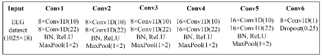
Figure 1: Proposed 1D CNN architecture.

III-B Factor Graph Based Inference

The 1D CNN model outputs an estimate of the probability that a given 4-seconds block corresponds to a seizure. This probability is based solely on its input EEG segment block, and does not account for the fact that the presence of a seizure in a given block is likely to also reflect on its preceding and subsequent blocks. To incorporate this temporal correlation, we combine the probability estimates over multiple blocks by assuming that the underlying temporal correlation can be represented using a factor graph, and utilize the sum-product method for inference [26]. In the following we first describe how the underlying dynamics of the seizure detection setup can be represented as a factor graph, after which we discuss the sum-product algorithm and elaborate on its combinations with the proposed 1-D CNN model.

III-B1 Factor Graph Representation of Underlying Dynamics

Factor graphs provide a visual representation of a multivariate function, typically a joint distribution measure, which can be factorized into a partition of local functions [20]. These partitions capture the inherent statistical relationship among variables affecting each partition. To represent a multivariate function as a factor graph, every partition and every variable must be associated with a unique node. Edges connect function nodes to variables nodes if and only if the function is explicitly dependent on the corresponding variable. We adopt the Forney style representation of factor graphs, where variable nodes are replaced by edges [27]. This graphical representation enables desired quantities to be computed at reduced complexity via message passing over the factor graph [20].

To implement factor graphs inference, we first fix the structure of the graph, i.e., the interconnection between its nodes, which encapsulates our knowledge on the underlying statistical relationships for the seizure detection problem. A key feature preceding epileptic seizures is the de-synchronization of its rhythmic activity [28]. To capture this behavior in our model study, we adopt a first-order HMM. The Markovian architecture focuses on the temporal characteristics associated with the epileptic episodes, highlights the effects of temporal correlations in seizure detection, and facilitates efficient classification at reduced complexity. The resulting factor graph under this model is illustrated in Fig. 2.

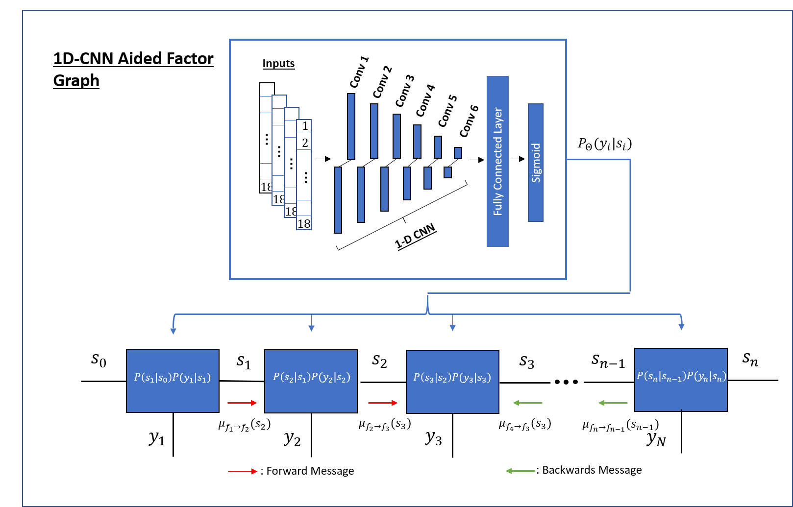
Figure 2: Factor Graph of a HMM with function nodes computed using a 1-D CNN.

To formulate this mathematically, let $\boldsymbol{y}=\{y_{1},y_{2},\cdots,y_{N}\}$, and $\boldsymbol{s}=\{s_{1},s_{2},\cdots,s_{N}\}$ describe the observed EEG measurements and latent seizure states, respectively, over $N$ consecutive 4-seconds blocks. The latent states takes binary values, i.e., $s_{i}\in\{0,1\}$ corresponding to the presence or absence of a seizure. We assume that these states satisfy the Markovian property, and use $P(s_{i}|s_{i-1})$ to denote the transition probability. The transition probability is taken as a control parameter, whose entries are fixed handcrafted values. In particular, we set $P(s_{i}=1|s_{i-1}=0)$ to correspond to a $10.46\%$ of switching from non-seizure to seizure, and $17.9\%$ for transitioning in the opposite direction. Ideally, one would like the transition probability matrix to reflect the true transitions probabilities between seizure and non-seizure state. However, the negligible seizure occurrences throughout the recording of EEG episodes, produces a highly unbalanced transition probabilities. Empirically, such transition probabilities did not facilitate accurate inference, hence hyper-parameter optimization of these probabilities was adopt, so that superior performance can be achieved. To close, we assume each EEG measurement depends only on its corresponding seizure state. Under this postulated HMM, the joint probability density function of the measurements and the states can be written as:

$$P(\boldsymbol{s},\boldsymbol{y})=\prod_{i=1}^{N}P(s_{i}|s_{i-1})P(y_{i}|s_{i}).$$ (1)

III-B2 The Sum-Product Algorithm

Having established the mathematical foundation and suitable factor graph representation, the objective is to distinguish between seizure and non-seizures states. Classification of these states is achieved through accurate inference of the marginal distribution $P(s_{i},\boldsymbol{y})$, which is the metric used to compute the maximum a-posteriori probability detector. In principle, evaluating $P(s_{i},\boldsymbol{y})$ from (1) involves marginalization; a task whose computational burden scales exponentially with $N$. However, by employing factor graph inference via the sum-product algorithm, the same computation scales only linearly with $N$, making this operation computationally feasible for the problem at hand.

The sum-product method relates the desired marginal probability to a product of "messages", where for each $k\in\{1,\ldots,N\}$ we write

$$P(s_{k},\boldsymbol{y})=\mu_{f_{j}\rightarrow s_{k}}(s_{k})\cdot\mu_{f_{j+1}\rightarrow s_{k}}(s_{k}).$$ (2)

The terms $\mu_{f_{j}\rightarrow s_{k}}(s_{k}),\mu_{f_{j+1}\rightarrow s_{k}}(s_{k})$ in (2) are interpreted as the "forward message" and "backward message" respectively, and are computed by [20]

$$\mu_{f_{j}\rightarrow s_{k}}(s_{k})=\sum_{\{s_{1},\cdots,s_{k-1}\}}\prod_{i=1}^{n}f_{i}(y_{i},s_{i},s_{i-1}),$$ (3)

and

$$\mu_{f_{j+1}\rightarrow s_{k}}(s_{k})=\sum_{\{s_{k+1},\cdots,s_{N}\}}\prod_{i=n+1}^{N}f_{i}(y_{i},s_{i},s_{i-1}),$$ (4)

where,

$$f_{i}(y_{i},s_{i},s_{i-1})=P(s_{i}|s_{i-1})P(y_{i}|s_{i}).$$ (5)

For a Markov chain factor graph structure as in Fig. 2, the computational complexity is comprised of evaluating the forward (3) and the backward (4) messages. The recursive nature of the computations implies that the number of FLOPs grows linearly with the number of $4$-second blocks in a given EEG episode, denoted by $N$. At the same time, the number of FLOPs also increases with the cardinality of the seizure state, denoted by $|\mathcal{S}|$, as well as the order of the Markov chain. Here, all seizure states are binary, hence $|S|=2$, and the factor graph is that of a first-order Markov chain. As a result, each message computation requires 4 multiplications and 2 addition operations. The result of these computations over a complete EEG episode requires merely $12N$ FLOPs, which is negligible compared to the complexity of applying the neural network models, as reported in Table I.

III-B3 CNN-Aided Factor Graphs

Implementing the sum-product algorithm requires knowledge of the underlying probability distribution $P(y_{i}|s_{i})$. In the case of seizure detection from EEG measurements, acquiring such a distribution from first principles is unattainable. Accurately characterizing epileptic seizures to high fidelity requires a combination of dynamical features and spatial-temporal features, for example the entropy, amplitude, synchronization, spectral power amongst other features associated with epileptic episodes, making the underlying distribution highly complex and intractable. To contend with this difficultly, we follow the work [29], combining DL models and inference algorithm. In particular, we utilize the output of the 1D CNN as an estimate of the conditional distribution $P(y_{i}|s_{i})$ required in order to compute the function nodes. via (5). Combining these approaches yields a hybrid model-based/data-driven detector, in which factor graph inference constitutes a robust final stage incorporating temporal correlation with the CNN outputs as illustrated in Fig. 2.

To complete the picture, the detection mechanism requires a comparison measure, i.e., a threshold, which represents a decision boundary for one to distinguish between different seizure states based on the estimated marginal distribution produced by the sum-product method. Treating the threshold as fixed, if the resultant probability of a seizure state yielded by the CNN-aided factor graph exceeds that of the applied threshold, then the system is said to be in a seizure state. Otherwise the system is said to be in a non-seizure state. As shown in the sequel, this approach allows to achieve accurate detection with controllable tradeoffs between detection and false alarm.

IV Results and Discussion

We now discuss our evaluation results in this section. We begin by defining the performance metrics we employed for evaluation followed by the results and the discussions.

IV-A Evaluation Method and Performance Metrics

We apply 6-fold leave-4-patient-out cross validation to evaluate the performance and the generalizability of our hybrid model-based/data-driven approach. Specifically, in each fold, 4 patients are kept for testing and 20 patients for training. The dataset used for evaluation, similar to train data, is segmented into 4-second blocks with moving window of 1 second where each block is labeled. To evaluate the performance of the models trained in each fold, we use the following metrics.

• F1-score: is a harmonic mean of recall and precision where former indicates the proportion of real positive cases that are correctly predicted positive and latter denotes the proportion of predicted positive cases that are correctly real positives [31].

• AUC-PR: is area under the precision-recall curve where high area under the curve means low false positive rate and low false negative rate.

• AUC-ROC is area under receiver operating characteristics (ROC) curve which is performance measurement for classification problems at various threshold settings.

We choose these performance measures since the data is imbalanced (i.e., for every block with seizure we have 6 blocks with no seizures, and AUC measures are great indicator of performance over imbalanced data.

TABLE II: Summary of Results

	AUC-ROC	AUC-PR	F1 score
2D CNN [16]	$87.27\pm 0.05$	$72.05\pm 11.46$	$85.58\pm 1.63$
2D CNN LOO [24]	N/A	N/A	$46.6\pm 31.0$
Our 1D CNN	$89.53\pm 0.04$	$74.53\pm 10.56$	$89.22\pm 2.36$
Our 1D CNN-FG	$90.23\pm 0.05$	$76.73\pm 11.44$	$90.55\pm 3.84$
Our 1D CNN-GRU	$90.56\pm 0.03$	$76.77\pm 8.05$	$90.42\pm 3.15$

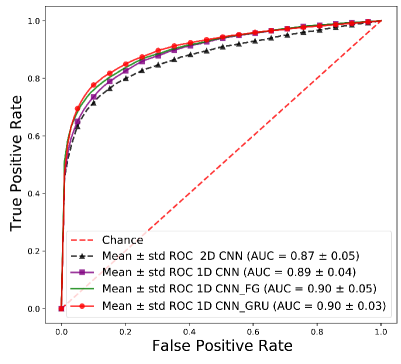
Figure 3: Area under ROC curve for all architectures.

IV-B Numerical Results

We consider 5 models for comparison. The baselines models from [16, 24], the 1D CNN we proposed, the CNN-aided factor graph, and the 1D CNN with GRU for capturing the temporal correlations. From the baseline models, we implement the exact architecture in [16] and evaluate it using the 6 fold leave-4-patient-out. For [24], since it uses images as features, we just report the results of their leave-one-patient-out (LOO) evaluations from their paper.

Fig. 3 shows the average AUC-ROC across the 6 folds, while Table II summarizes all the results. As can be seen, changing the model from 2D CNN proposed in [16] to our proposed 1D CNN architecture results in approximately 2% improvement across all performance measure. Our hybrid model-based/data-driven CNN-aided factor graph further improves the results by as much as 2%. Compared to [24], we perform a leave-4-patient-out evaluation as opposed to leave-one-patient-out. This reduces the number of patients we use for training compared to [24]. Despite this reduction, we achieve a much higher F1 score compared to [24] as shown in Table II. Moreover, while AUC-PR is not reported in [24], the precision of $51.4\pm 34.1$ and recall of $53.1\pm 25.5$ is reported, which is significantly lower than the performance achieved by our proposed approach.

The 1D CNN with GRU achieves the same performance as our proposed CNN-aided factor graph inference method for all performance metrics. This demonstrates that the hybrid model-based/data-driven approach proposed here can achieve similar performance as a purely data-driven methods that employ deep and highly parameterized neural networks. This performance is achieved by our CNN-aided factor graph at a fraction of the computational complexity of deep learning based approaches as summarized in Table I. This makes the proposed method suitable for real-time seizure detection.

V Conclusions

In this paper, we proposed a computationally efficient hybrid model-based/data-driven method using CNN-aided factor graphs for seizure detection. First, we carefully designed a 1D CNN for estimating the probability that a 4-second block of EEG recording is a seizure block. We then used this neural network in the factor node of the factor graph for inference. We demonstrated that the proposed method generalizes well to other patients using a 6-fold leave-4-patient-out cross validation. We also showed that our algorithm achieves up to 5% improvement in performance compared to prior work, while maintaining much lower computational complexity. This makes our approach ideal for real-time seizure detection. For future work, we plan to expand our approach to classifying focal and generalized seizures since this is a challenging task in clinical procedures.

References

- [1] “Epilepsy.” https://www.who.int/news-room/fact-sheets/detail/epilepsy.
- [2] C. Park, G. Choi, J. Kim, S. Kim, T.-J. Kim, K. Min, K.-Y. Jung, and J. Chong, “Epileptic seizure detection for multi-channel EEG with deep convolutional neural network,” in International Conference on Electronics, Information, and Communication (ICEIC), 2018.
- [3] G. Zazzaro, S. Cuomo, A. Martone, R. V. Montaquila, G. Toraldo, and L. Pavone, “EEG signal analysis for epileptic seizures detection by applying data mining techniques,” Internet of Things, vol. 14, p. 100048, 2021.
- [4] S. Kulaseharan, A. Aminpour, M. Ebrahimi, and E. Widjaja, “Identifying lesions in paediatric epilepsy using morphometric and textural analysis of magnetic resonance images,” NeuroImage: Clinical, vol. 21, 2019.
- [5] N. van Klink, A. Mooij, G. Huiskamp, C. Ferrier, K. Braun, A. Hillebrand, and M. Zijlmans, “Simultaneous MEG and EEG to detect ripples in people with focal epilepsy,” Clinical Neurophysiology, vol. 130, no. 7, pp. 1175–1183, 2019.
- [6] N. Pianou and S. Chatziioannou, “Imaging with PET/CT in Patients with Epilepsy,” in Epilepsy Surgery and Intrinsic Brain Tumor Surgery, pp. 45–50, Springer, 2019.
- [7] A. Subasi, J. Kevric, and M. Abdullah Canbaz, “Epileptic seizure detection using hybrid machine learning methods,” Neural Computing and Applications, vol. 31, pp. 317–325, Jan. 2019.
- [8] M. Golmohammadi, S. Ziyabari, V. Shah, S. L. de Diego, I. Obeid, and J. Picone, “Deep architectures for automated seizure detection in scalp EEGs,” arXiv preprint arXiv:1712.09776, 2017.
- [9] I. B. Slimen, L. Boubchir, Z. Mbarki, and H. Seddik, “EEG epileptic seizure detection and classification based on dual-tree complex wavelet transform and machine learning algorithms,” Journal of biomedical research, vol. 34, no. 3, p. 151, 2020.
- [10] S. R. R. Ahmad, S. M. Sayeed, Z. Ahmed, N. M. Siddique, and M. Z. Parvez, “Prediction of epileptic seizures using support vector machine and regularization,” in 2020 IEEE Region 10 Symposium (TENSYMP), pp. 1217–1220, IEEE, 2020.
- [11] S. Raghu, N. Sriraam, S. V. Rao, A. S. Hegde, and P. L. Kubben, “Automated detection of epileptic seizures using successive decomposition index and support vector machine classifier in long-term EEG,” Neural Computing and Applications, vol. 32, no. 13, pp. 8965–8984, 2020.
- [12] C. Li, W. Zhou, G. Liu, Y. Zhang, M. Geng, Z. Liu, S. Wang, and W. Shang, “Seizure Onset Detection Using Empirical Mode Decomposition and Common Spatial Pattern,” IEEE Transactions on Neural Systems and Rehabilitation Engineering, vol. 29, pp. 458–467, 2021.
- [13] S. Khalilpour, A. Ranjbar, M. B. Menhaj, and A. Sandooghdar, “Application of 1-D CNN to predict epileptic seizures using EEG records,” in 2020 6th International Conference on Web Research (ICWR), pp. 314–318, IEEE, 2020.
- [14] G. C. Jana, R. Sharma, and A. Agrawal, “A 1D-CNN-spectrogram based approach for seizure detection from EEG signal,” Procedia Computer Science, vol. 167, pp. 403–412, 2020. Publisher: Elsevier.
- [15] R. V. Sharan and S. Berkovsky, “Epileptic seizure detection using multi-channel EEG wavelet power spectra and 1-D convolutional neural networks,” in 2020 42nd Annual International Conference of the IEEE Engineering in Medicine & Biology Society (EMBC), pp. 545–548, IEEE, 2020.
- [16] P. Boonyakitanont, A. Lek-uthai, K. Chomtho, and J. Songsiri, “A Comparison of Deep Neural Networks for Seizure Detection in EEG Signals,” bioRxiv, p. 702654, 2019.
- [17] S. Roy, I. Kiral-Kornek, and S. Harrer, “Deep learning enabled automatic abnormal EEG identification,” in International Conference of the IEEE Engineering in Medicine and Biology Society (EMBC), pp. 2756–2759, 2018.
- [18] W. Liang, H. Pei, Q. Cai, and Y. Wang, “Scalp EEG epileptogenic zone recognition and localization based on long-term recurrent convolutional network,” Neurocomputing, vol. 396, pp. 569–576, 2020.
- [19] M. Lee, I. Youn, J. Ryu, and D.-H. Kim, “Classification of both seizure and non-seizure based on EEG signals using hidden Markov model,” in 2018 IEEE International Conference on Big Data and Smart Computing (BigComp), pp. 469–474, IEEE, 2018.
- [20] H.-A. Loeliger, “An introduction to factor graphs,” IEEE Signal Process. Mag., vol. 21, no. 1, pp. 28–41, 2004.
- [21] P. D. Emmady and A. C. Anilkumar, “EEG, Abnormal Waveforms,” StatPearls [Internet], 2020.
- [22] A. L. Goldberger, L. A. Amaral, L. Glass, J. M. Hausdorff, P. C. Ivanov, R. G. Mark, J. E. Mietus, G. B. Moody, C.-K. Peng, and H. E. Stanley, “PhysioBank, PhysioToolkit, and PhysioNet: components of a new research resource for complex physiologic signals,” circulation, vol. 101, no. 23, pp. e215–e220, 2000.
- [23] W. Klonowski, “Everything you wanted to ask about eeg but were afraid to get the right answer,” Nonlinear biomedical physics, vol. 3, no. 1, pp. 1–5, 2009.
- [24] C. Gomez, P. Arbelaez, M. Navarrete, C. Alvarado-Rojas, M. Le Van Quyen, and M. Valderrama, “Automatic seizure detection based on imaged-EEG signals through fully convolutional networks,” Scientific Reports, vol. 10, p. 21833, Dec. 2020.
- [25] K.-O. Cho and H.-J. Jang, “Comparison of different input modalities and network structures for deep learning-based seizure detection,” Scientific Reports, vol. 10, p. 122, Jan. 2020.
- [26] F. R. Kschischang, B. J. Frey, and H.-A. Loeliger, “Factor graphs and the sum-product algorithm,” IEEE Trans. Inf. Theory, vol. 47, no. 2, pp. 498–519, 2001.
- [27] G. D. Forney, “Codes on graphs: Normal realizations,” IEEE Trans. Inf. Theory, vol. 47, pp. 520–548, 2001.
- [28] F. Mormann, T. Kreuz, R. G. Andrzejak, P. David, K. Lehnertz, and C. E. Elger, “Epileptic seizures are preceded by a decrease in synchronization,” Epilepsy research, vol. 53, no. 3, pp. 173–185, 2003.
- [29] N. Shlezinger, N. Farsad, Y. C. Eldar, and A. J. Goldsmith, “Learned factor graphs for inference from stationary time sequences,” arXiv preprint arXiv:2006.03258, 2020.
- [30] N. Shlezinger, N. Farsad, Y. C. Eldar, and A. J. Goldsmith, “ViterbiNet: A deep learning based Viterbi algorithm for symbol detection,” IEEE Trans. Wireless Commun., vol. 19, no. 5, pp. 3319–3331, 2020.
- [31] D. M. Powers, “Evaluation: from precision, recall and F-measure to ROC, informedness, markedness and correlation,” arXiv preprint arXiv:2010.16061, 2020.