Kinetic Fragility Directly Correlates with the Many-body Static Amorphous Order in Glass-Forming Liquids

Abstract

The term “fragility” describes the rate at which viscosity grows when a supercooled liquid approaches its putative glass transition temperature. The field of glassy materials is actively searching for a structural origin that governs this dynamical slowing down in the supercooled liquid, which occurs without any discernible change in structure. Our work shows clear evidence that growing many-body static amorphous order is intimately correlated with the kinetic fragility of glass-forming liquids. It confirms that the system’s dynamical response to temperature is concealed in its micro-structures. This finding may pave the way for a deeper understanding of the different temperature dependence of the relaxation time or viscosity in a wide variety of glass-forming liquids.

Introduction: The dramatic rise in viscosity or relaxation time upon supercooling is a universal hallmark feature across all glass-forming liquids. Despite extensive investigations Berthier1797 ; RevModPhys.83.587 ; doi:10.1146/annurev-conmatphys-031113-133848 ; PhysRevLett.121.085703 ; doi:10.1063/1.5033555 ; Tahacsomega , one of the fundamentally unsolved challenges in condensed matter physics is understanding of microscopic origin of rapid rise in viscosity ($\eta$) with relatively small temperature changes while approaching the calorimetric glass transition temperature ($T_{g}$), defined as the temperature at which $\eta$ becomes $10^{14}Poise$. In this context, it’s also worth noting that, while near-diverging growth of viscosity is universal in all glass-forming liquids, the rate at which viscosity grows at low temperatures is quite non-universal and varies significantly across liquids.

The term “fragility” was first coined in Ref. Angell1924 to characterize this rapid non-universal changes in viscosity near $T_{g}$. Although, the word “fragility” is used to describe the dynamical properties, several theoretical and experimental studies sastry_nature ; Martineznature ; Kaori_nature ; Debenedetti ; Mauronatcomm ; doi:10.1063/1.4964362 demonstrate that the fragility is fundamentally connected to thermodynamic properties of the liquid, like the excess entropy and the specific heat which are directly linked with the microscopic structure of a liquid. This connection led to a search for the structural or thermodynamic correlations in these amorphous systems, which may qualitatively describe the source of fragility. However, the correlation between thermodynamics and dynamical properties in supercooled liquids remains somewhat controversial, leading to inherent uncertainty, which prevents researchers from reaching a consensus. Thus, to establish a definitive correlation between thermodynamic properties and kinetic fragility further research will be welcomed. The outcome will certainly have significant implications in understanding some of these puzzles in the dynamics of supercooled liquids. In this article, we have addressed the connection between growing static amorphous order and fragility by performing extensive molecular dynamics simulations of a model glass-forming liquid, showing very large variation in fragility with increasing density.

The temperature dependence of viscosity and relaxation time for a wide variety of supercooled liquids can be well fitted by the Vogel-Fulcher-Tamann (VFT) formula 10004192038 ; https://doi.org/10.1111/j.1151-2916.1925.tb16731.x ; https://doi.org/10.1002/zaac.19261560121 :

$$\tau_{\alpha}(T)=\tau_{0}\exp\left[\frac{1}{K_{VFT}\ (T/T_{VFT}-1)}\right],$$ (1)

where $\tau_{\alpha}$ is the structural relaxation time (defined later), $\tau_{0}$ is the viscosity at infinite high temperature, $T_{VFT}$ is the apparent divergence temperature for relaxation time and $K_{VFT}$ denotes the “Kinetic fragility”. The fragility index provides a unifying framework for the classification of a broad range of systems, from molecular liquids Angell1924 to colloidal Frag_Molecu and biological systems Sussman_2018 ; D0SM01575J . Additionally, material functionality and manufacturability are directly linked with their fragility index. Like the system that have low fragility index, generally implies to have a wide glass transition temperature range which enhances the flexibility of material moulding. Moreover, material bulk properties depend on its molecular mechanisms and an important question is how the molecular mechanisms of glass forming liquids differ from each other in such a way that their dynamic properties vary so widely. Fragility also plays important role in bio-preservationFox1922 ; https://doi.org/10.1111/j.1365-2621.1991.tb07970.x ; doi:10.1063/1.5085077 . Empirical evidence suggests that the larger the fragility of a liquid, the better it will be in preserving biomacromolecules when used as a medium. Although, there are deviations from this hypothesis but this remained as a rule of thumb in bio-preservation industry. Thus, a better understanding of fragility may lead to better understanding of the physics of biopreservation.

Models and Methods: To gain valuable insights into molecular mechanisms and explore the connection between length scales associated with liquid structure and fragility, we have performed extensive computer simulations of soft repulsive particles PhysRevLett.88.075507 ; doi:10.1146/annurev-conmatphys-070909-104045 ; Berthier_2009 by varying the density, $(\rho)$, and temperature, $(T)$, which cover a broad spectrum of fragility. This model (referred as HP model) shows a strong crossover from strong glass to fragile glass behaviour with varying density $(\rho)$ beyond the jamming density $(\rho_{J})$ Berthier_2009 . This provides a conceptual and more feasible way to tune fragility without changing the particle composition, interaction potential or curving the configurational space PhysRevLett.101.155701 . Simulations are done in three-dimensions in the density range $\rho\in[0.65,0.82]$ with $N=108000$ particles. More detailed information about the models and simulations is provided in SI SI . To describe the dynamics of the system, we have computed the average relaxation timescale, $\tau_{\alpha}$, of the system via the two-point overlap correlation function $(Q(t))$ (defined in the SI SI ) at each equilibrium density, $\rho$, and temperature, $T$ state points. The relaxation time $\tau_{\alpha}$ is defined as $\langle Q(\tau_{\alpha})\rangle=1/e$, where $\langle\cdots\rangle$ refers to ensemble average. The calorimetric glass transition temperature, $T_{g}$ for this model in simulations is defined as $\tau_{\alpha}(T_{g})=5\times 10^{6}$.

Results:

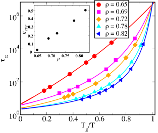
Figure 1: Angell plot of $(\tau_{\alpha})$ as a function of rescaled temperature, $T_{g}/T$ at different densities ($\rho$). At higher density the relaxation time exhibits a sharp growth upon decreasing temperature, a feature of a fragile glass-former, while at lower density the relaxation time displays Arrhenius behaviour with temperature, suggesting a crossover to strong glass-former. Lines are the fit to VFT form. Inset shows the fragility index against density.

Fig. 1 shows the Angell plot of the relaxation time $(\tau_{\alpha})$ as a function of rescaled inverse temperature. To have a fair comparison, the data has been normalized by respective $T_{g}$ at different density. At low density the relaxation time exhibits Arrhenius dependence, indicating a behaviour of a strong glass forming liquid, whereas at high density the relaxation time display super-Arrhenius temperature dependence, often referred as “Fragile glass-former”. In these models, fragility can be tuned over a broad range, by only increasing the density without changing any other microscopic characteristics of the systems. This gives us a big opportunity to look into the precise molecular mechanisms that cause such large change in fragility. In the inset of Fig. 1, we plot the fragility index $(K_{VFT})$ against density. One can see that increasing bulk density by a factor of $1.26$ ($\rho=0.65$ to $0.82$) changes the kinetic fragility by a factor of $17$ ($K_{VFT}=0.0295$ to $0.5002$). Thus this model is an ideal test-bed for deciphering the microscopic origin of fragility and its possible connection to growing amorphous order as envisaged in Random First Order Transition (RFOT) Theory PhysRevA.40.1045 ; doi:10.1146/annurev.physchem.58.032806.104653 . In the subsequent paragraphs, we will discuss the strong correlation between changing fragility and the two important growing length scales in the systems; namely dynamic heterogeneity length scale ($\xi_{d}$) and static amorphous order length scale ($\xi_{s}$).

Dynamic Length Scale: Since, fragility is measured from dynamical properties like relaxation time, it is natural to investigate the temperature dependence of $\xi_{d}$ for these model systems and try to understand a possible correlation between them. Recent work doi:10.1063/1.4938082 pointed out that growth of dynamic heterogeneity (DH) in strong liquids is different than in fragile liquids. Thus, a systematic study of DH doi:10.1146/annurev.physchem.51.1.99 in this current set up is indeed warranted to have a detailed understanding of how heterogeneity gets affected by changing fragility in the system. DH can be quantified via the fluctuation of two-point correlation function (Q(t)) PhysRevE.66.030101 and the length scale associated with DH, can be measured from the spatial correlation of four-point structure factor (fluctuation of two point correlation function in fourier space, $S_{4}(q,t=\tau_{\alpha})$) PhysRevE.58.3515 ; doi:10.1063/1.1605094 . In SI SI , the determination of $\xi_{d}$ from $S_{4}(q,t=\tau_{\alpha})$ has been elaborated. Recently, in Ref. PhysRevLett.119.205502 , another method of extracting dynamic length scale has been proposed. In this method the dynamical properties of the systems is measured at a smaller sub volume of the systems by diving the whole systems in to smaller blocks of length, $L_{B}$. This method can be easily implemented both in experiments and in numerical simulations and termed as “block analysis” method. The method has also been shown to significantly improve the statistical averaging of the data as well as include all possible fluctuations (e.g density, temperature, composition, etc.) that are important in measuring four-point correlation functions (see SI SI for further details). We have obtained the dynamic length scales using both the methods for reliability.

In Fig. 2(a), we show a comparison of the dynamic length scales obtained using two different methods for systems which reside on the two extreme ends of the spectrum in the Angell plot; first one being the most fragile liquid with $\rho=0.82$ (see Fig. 2(a)), while the other is at the strong liquid end (Fig. 2(a) inset) with $\rho=0.65$. The quite good agreement between these two ways of estimations of $\xi_{d}$ for all state points provides us confidence in the measured heterogeneity length scale.

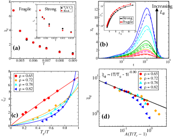
Figure 2: (a). Dynamics length scale as a function of temperature for fragile liquid. The legend shows the method of extraction of length scale. Similar plot for strong glass forming liquid is shown in the inset. (b). Dynamical heterogeneity as a function of time for various block size ($L_{B}$). Fragile liquids ($\rho=0.82$, solid lines), shows stronger growth of dynamic heterogeneity compare to strong liquids ($\rho=0.65$, dotted lines). We display $\chi_{4}(t)$ for the strong and fragile liquids at roughly the same block scale. Fragile liquids display more heterogeneity than strong liquids at a given block size. The maximum of $\chi_{4}(t)$ ($\chi_{4}^{P}$) for fragile and solid liquids at the same relaxation time $(\tau_{\alpha})$ is shown in the inset as a function of block size $(L_{B})$. (c). Dynamic length scales as a function of rescaled temperature by $T_{g}$. Solid lines are fits to the form $\xi_{d}\sim|T/T_{VFT}-1|^{-\nu}$. (d). Dynamic length scales are plotted as a function of $|T/T_{c}-1|$, where $T_{c}$ is the MCT divergence temperature. The length scale data are rescaled to make it more comparable to other data sets. The black line is a power fit with an exponent $\nu=0.30$ (see text for discussion).

An interesting question that naturally comes up is the following: if the two extreme systems (strong and fragile) have very similar structural relaxation times, do they have similar dynamic heterogeneity? To investigate this we plot $\chi_{4}$ as a function of time in Fig. 2(b) for strong and fragile liquid ($\tau_{\alpha}$ for these two systems are close to each other) at roughly the same block size $(L_{B})$. We find that fragile liquid show stronger dynamic heterogeneity than strong liquid for a given block size. In the inset of Fig. 2(b), we plot the peak value of $\chi_{4}(t)$ as a function of $L_{B}$ for these two extreme systems at the same $\tau_{\alpha}$. Fragile liquid shows stronger dynamic heterogeneity at each length scale than the strong glass-former. This observation is in stark contrast with a recent finding paul2021dynamic of possible decoupling of relaxation time and dynamic heterogeneity in active glass-forming liquids. There we observed that heterogeneity increase with decreasing fragility if the relaxation time is kept constant. Next we focus on the temperature dependence of $\xi_{d}$ with changing fragility. Fig. 2(c) shows the growth of dynamic length scale as a function $T_{g}/T$. It can be seen that for the fragile glass former, $\xi_{d}$ shows a sharp growth upon supercooling, whereas strong glass former produces a gentle growth resembling the Angell like plot for $\tau_{\alpha}$ (see Fig.1).

Inhomogeneous mode coupling theory (IMCT) PhysRevLett.97.195701 predicts that three-point density correlation function, $\chi_{3}(t)$, which can be obtained by measuring the response of the system under an external perturbation, is intimately related to the four-point susceptibility $\chi_{4}(t)$ and shows similarly scaling behaviour near the MCT transition temperature ($T_{c}$). Thus, according to IMCT, $\xi_{d}$ should have a critical like behaviour: as $\xi_{d}\sim|T-T_{c}|^{-\nu}$ with $\nu=1/4$ being the predicted critical exponent. Recently, Tah et.al, PhysRevResearch.2.022067 showed for few model glass forming liquids that the exponent $\nu$ is in agreement with IMCT prediction for temperature near $T_{c}$. However, validity of this result across a wide range of systems with changing fragility is not studied before. In Fig. 2(d) we show the dependence of $\xi_{d}$ vs $(T-T_{c})/T_{c}$ for different fragile systems. The black line shows the power law fit to the few low temperature data points. We find for all the different fragile systems the value of the exponent is $\sim 0.30$ (near $T_{c}$) which is not very different from the exponent $\nu=0.25$ expected by IMCT. The small difference in exponent may be attributable to the finite dimensions, and understanding how the exponent shifts in higher dimensions (e.g. near the upper critical dimension $d_{c}=8$) PhysRevE.81.040501 ; Charbonneau13939 ; Franz18725 , will be of considerable interest.

Amorphous order and Fragility: The lack of a priori knowledge of the nature of the structural order in disorder glass forming liquids makes it difficult to measure the relevant degree of order. However, existing results show that the system has domains of different mobility near the glass transition temperature and these domains have relaxation rates that are substantially faster or slower than the system’s average relaxation rate. These different domains often called as “ cooperatively rearranging regions (CRRs)”, are the primary building blocks of the phenomenological Adam-Gibbs theory 1965JChPh..43..139A of glass transition and its subsequent development, i.e., the random first-order transition (RFOT) theory PhysRevA.40.1045 ; doi:10.1146/annurev.physchem.58.032806.104653 . Different mobility domains have different patch entropy, and the mean patch correlation length can be easily extracted from the largest groups of congruent patches which are considered to have a similar local order PhysRevLett.107.045501 . This hints that the origins of heterogeneous dynamics may be buried in the local amorphous structure. Bouchaud and Biroli doi:10.1063/1.1796231 suggested a non-trivial correlation function known as point-to-set (PTS) correlation Natphy2008 to calculate the structural or thermodynamic correlation length scale in supercooled glass-forming liquids in an order-agnostic way as envisaged in RFOT theory. Growth of this static length scale gives a notion of emerging thermodynamic order that may be connected to the dynamical slowing down of the system, even when traditional structural features (e.g. “pair correlation function”) are blind to capture the dramatic slowing down of the relaxation time. Here, we address the crucial question of whether the growing thermodynamic amorphous order can universally explain the origin of a wide spectrum of fragility.

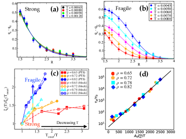
Figure 3: Overlap correlation as a function of cavity radius $R$ for strong glass former (a) and fragile glass former (b) at various temperatures. (c) Rescaled static length scale ($\xi_{s}$) as a function of reduced temperature (re-scaled by onset temperature $(T_{onset})$). Here, $\xi_{s}(T_{onset})$ is the value of static length scale at onset temperature. (d) Rescaled relaxation time $(\tau_{\alpha}/\tau_{0})$ as a function of $\xi_{s}^{\psi}/T$ yielded a good data collapse for all the different fragile liquids.

To address this, we have computed the static length scale using point-to-set correlation function in cavity geometry (see the SI SI ) Natphy2008 ; PhysRevLett.108.225506 ; PhysRevLett.121.085703 ; Nagamanasa ; PhysRevE.94.032605 . Fig. 3(a) and 3(b) show the nature of the correlation function with increasing cavity radius, $R$ for various studied temperatures for a strong and a fragile liquid. The correlation functions for the strong liquid decay at the same rate for all temperatures, indicating no growth in the amorphous order (see Fig. 3(a)) with decreasing temperature. However, for fragile liquid these correlation functions show significantly slower decay as a function of $R$ with decreasing temperature. The estimation of the length scale $(\xi_{s})$ can be done by simply fitting the correlation functions (see SI for details). We also extracted the static length scale using block analysis of relaxation time as proposed in Ref. PhysRevLett.119.205502 (see SI SI for details). The temperature dependence of the length scale for different fragile liquids determined by point-to-set method and block analysis method are shown and compared in Fig. 3(c). We find that the length scales obtained by these two methods are very similar for all the studied systems. For better representation, we rescaled the static length scale by its value at onset temperature (temperature at which the thermodynamic and dynamic properties begin to depart from its high temperature behaviour B008749L ) and show the data only for temperatures below the onset temperature (see SI). For strong glass forming liquid $\xi_{s}$ (“red squares”) does not grow much with decreasing temperature, but for fragile glass forming liquid it (“blue circles”) grows sharply as system approaches the glass transition temperature.

Within the RFOT scenario, the structural relaxation time of a system is related to $\xi_{s}$ as

$$\tau_{\alpha}(T)=\tau_{0}\exp\left[\frac{\Delta_{0}\ \xi_{s}^{\psi}(T)}{T}\right],$$ (2)

where typical free energy barrier is $\Delta(T)=\Delta_{0}\ \xi_{s}^{\psi}(T)$ with $\psi$ being an apriori unknown scaling exponent. $\Delta_{0}$ and $\tau_{0}$ set the energy scale and microscopic time scale of the system. Thus, according to Fig. 3(c), the typical free energy barrier for a strong glass former remains nearly constant as $\xi_{s}$ (red squares) stays nearly constant, but rises (blue circles) sharply for a fragile liquid as the temperature is lowered towards $T_{g}$, resulting in super-Arrhenius behaviour. We believe this is the first numerical evidence that conclusively suggest that $\xi_{s}$ which was first introduced in the RFOT theory to characterize the liquid’s mosaic order, controls the relaxation process including the drastic change in fragility with changing density in supercooled liquids. We also believe the above results are very general and constitute a first clear demonstration that order agnostic thermodynamic order (applicable to all generic glass formers) is strongly correlated to fragility, rather than some specific locally preferred structure (LFS) doi:10.1063/1.2773716 ; Hallett ; PhysRevX.8.011041 .

Now, if $\tau_{\alpha}$ is solely depended on the thermodynamics length scales as given in Eq.2, then one should be collapsed all the data of relaxation time for all the systems with varying fragility on to a master curve if plotted against $\xi_{s}^{\psi}/T$. To validate the above argument we plotted the re-scaled relaxation time $(\tau_{\alpha}/\tau_{0})$ (re-scaled by time scale $(\tau_{0})$ at very high temperature where $\xi_{s}\to 0$) as a function of $\Delta_{0}\xi_{s}^{\psi}(T)/T$ and find that data for all the systems with different fragility collapses on to a straight line as shown in Fig. 3 (d). We keep the exponent $\psi=2.6$ same while varying $\Delta_{0}$. Good data collapse implies an encouraging universality between the relaxation time and the static length scale across systems with large change in fragility. This implies that probably system’s dynamic heterogeneity is tied to the static length scale PhysRevLett.121.085703 ; doi:10.1146/annurev-conmatphys-031113-133848 .

Conclusion: Taken together, our findings show that by fine-tuning the system’s packing fraction, one might achieve a bigger change in kinetic fragility in soft repulsive systems for delving deeper into the relationship between their kinetic fragility and the microscopic structural ordering. This could be easily tested experimentally by using colloidal suspensions Johan_Nature . The heterogeneity length scale for fragile liquid increases significantly faster as the system approaches the glass transition temperature, whereas strong liquid shows much smaller increase. All liquids show MCT critical like behavior near the MCT temperature $(T_{c})$, with an exponent $\nu=0.30$ that is close to the exponent anticipated by IMCT theory. This suggests that all supercooled liquids with a wide range of kinetic fragility have a universal behavior in their dynamic heterogeneity. Finally, we show that the distinct temperature dependence of the order agnostic thermodynamics length scale controls the temperature dependence of the structural relaxation time for all the fragile liquid and suggests that widely different temperature dependency of structural relaxation in various glass-forming liquids is concealed in local amorphous order, whose growth determines whether a system will be strong to fragile glass formers. Since the material durability is an intrinsic property that is tightly linked to its fragility index, we expect that our findings will be useful to better understand the role of microscopic structure in the emergence of fragility in future.

IT thanks S. Ridout and A. J. Liu for discussions. IT wants to acknowledge use of Extreme Science and Engineering Discovery Environment (XSEDE) xsede , which is supported by National Science Foundation grant number TG-BIO200091. SK would like to acknowledge funding by intramural funds at TIFR Hyderabad from the Department of Atomic Energy (DAE). Support from Swarna Jayanti Fellowship grants DST/SJF/PSA-01/2018-19 and SB/SFJ/2019-20/05 are also acknowledged

Availability of Data

The data that support the findings of this study are available from the corresponding author upon reasonable request.

Supporting Information: Kinetic Fragility Directly Correlates with the Many-body Static Amorphous Order in Glass-Forming Liquids

I Models and Simulation Details

We have studied a few model glass forming liquids in three dimensions. The model details are given below:

3dHP Model:

We have done equilibrium molecular dynamics (MD) simulations of three-dimensional systems which interpolate between finite-temperature glasses and hard-sphere glasses and have been studied widely in the field of jamming physics PhysRevLett.88.075507,doi:10.1146/annurev-conmatphys-070909-104045. The system consists of $50:50$ binary mixture of $N$ particles and interacting via the following pair-wise potential

$$V_{\alpha\beta}(r)=\epsilon_{\alpha\beta}\left(1-\frac{r}{\sigma_{\alpha\beta}}\right)^{2}$$ (1)

for $r<\sigma_{\alpha\beta}$ and $V_{\alpha\beta}(r)=0$ otherwise. Here $(\sigma_{\alpha\alpha},\sigma_{\alpha\beta},\sigma_{\beta\beta})$ = $(1.00,\ 1.20,\ 1.40)$, and ($\epsilon_{\alpha\alpha},\epsilon_{\alpha\beta},\epsilon_{\beta\beta})=(1.0,\ 1.0,\ 1.0).$ The packing fraction is defined as $\phi=\frac{\pi}{12}(\sigma_{\alpha}^{3}+\sigma_{\beta}^{3})\rho$ and $\rho=N/L^{3}$ is the number density. We have used system sizes of $N=100$ to $N=108000$ particles in our MD simulations with periodic boundary conditions. We performed simulations in the density range $\rho\in[0.65,0.82]$. The system shows incipient crystallization above packing fraction $\phi=0.924$ $(\rho=0.94)$ Berthier_2009, which is well above the area of interest in our study. All reported results are in thermal equilibrium which have been carefully reviewed.

II Self overlap correlation function

The self overlap correlation function or two point overlap correlation function is defined as,

$$Q(t)=\frac{1}{N}\sum_{i=1}^{N}w\big{(}|\vec{r}_{i}(t)-\vec{r}_{i}(0)|\big{)},$$ (2)

where $w(x)$ is a window function defined as $w(x)=1$, if $x<a$ and $0$ otherwise. The window function $w(x)$ has been introduced to remove the decorrelation arising from particles’ vibrational motions inside the local cages that are formed by their neighbours. In our study, we choose $a=0.3$ which corresponds to the plateau value of the mean square displacement. However, the reported results are not very sensitive to the particular choice of $``a"$, as long as $``a"$ does not differ significantly from the above mentioned value. The relaxation time $\tau_{\alpha}$ is defined as $\langle Q(\tau_{\alpha})\rangle=1/e$, where $\langle\cdots\rangle$ refers to ensemble average.

III Methods to obtain dynamic length scale

III.1 Block analysis method

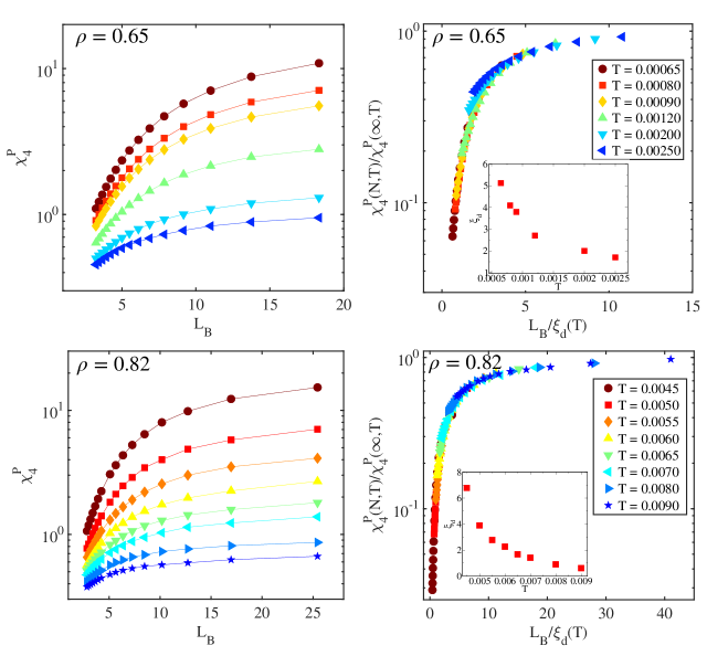
Figure S1: Top Panel: Block size dependence of $\chi_{4}^{P}$ (left panel) and its scaling collapse (right panel) to get the dynamic length scale $(\xi_{d}(T))$ for strong liquid $(\rho=0.65)$. Bottom panel: Similar plot for fragile liquid $(\rho=0.82)$.

Following the procedures of Ref. PhysRevLett.119.205502, we calculated the dynamic length scale from the finite size scaling of four-point susceptibility $(\chi_{4}(L_{B},t))$, where $L_{B}$ is the varying block size and $t$ is the measurement time. $\chi_{4}(L_{B},t)$ quantifies the fluctuation of two-point correlation function $Q(L_{B},t)$ for a given coarsening block of size $L_{B}$ and is defined as

$$\begin{split}\chi_{4}(L_{B},t)=N_{B}\left(\langle Q(L_{B},t)^{2}\rangle-\langle Q(L_{B},t)\rangle^{2}\right),\\ \text{and}\\ Q(L_{B},t)=\frac{1}{N_{B}}\sum_{i=1}^{N_{B}}\frac{1}{n_{j}}\sum_{j=1}^{n_{j}}w(|r_{j}(0)-r_{j}(t)|).\end{split}$$ (3)

$Q(L_{B},t)$ gives positional overlap between two configurations in a block of size $L_{B}$ separated by a time interval $t$. $N_{B}$ is the number of blocks of size $L_{B}$ and $n_{j}$ is the number of particles in that block at time $t=0$. In this analysis, we have evaluated the $\chi_{4}^{P}(L_{B},t)$ at the time interval close to $\sim\tau_{\alpha}$, system’s structural relaxation time, to perform the finite size scaling (FSS). Note that the system’s dynamics have the maximum heterogeneity near $t\sim\tau_{\alpha}$.

Now to obtain the dynamic length scale we perform finite size scaling of peak of four point dynamic susceptibility $\chi_{4}^{P}(L_{B},T)$, which varies systematically as the temperature drops and block size grows, implying an increasing length scale, and the data was found to be well described by the following scaling function,

$$\chi_{4}^{P}(L_{B},T)=\chi_{4}^{P}(\infty,T)\mathcal{F}\left[\frac{L_{B}}{\xi_{d}(T)}\right],$$ (4)

where $\chi_{4}^{P}(\infty,T)$ is the asymptotic value of $\chi_{4}^{P}(L_{B},T)$. The dynamics length scale $(\xi_{d})$ of the system can be obtained very reliably by performing data collapse to a master curve. In Fig. S1 we plot the block size dependence of $\chi_{4}(L_{B},T)$ and its scaling collapse of two extreme systems, one of which show strong liquid behaviour with $\rho=0.65$ (top panel of Fig. S1), while the other is at the most fragile liquid with $\rho=0.82$ (bottom panel of Fig. S1). In the inset of Fig. S1 we show the temperature dependence of the dynamics length scale for the two systems.

III.2 Calculation of dynamical length scale from four-point structure factor $S_{4}(q,t)$

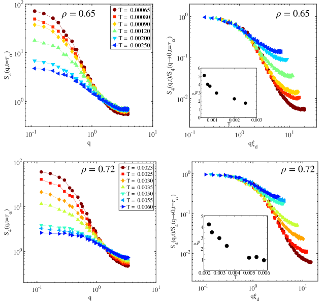
Figure S2: Top Left Panel: Dynamic structure factor $(S_{4}(q,t=\tau_{\alpha}))$ for $\rho=0.65$ as a function of wave vector $(q)$ for different temperature . Top Right Panel: Scaling plot $S_{4}(q,t)/S_{4}(q\to 0,t=\tau_{\alpha})$ vs $q\xi_{d}$ for the 108000 particle simulations. Bottom Panel: Similar plot for $\rho=0.72$. The dynamic length scale as a function of temperature is shown in the inset.

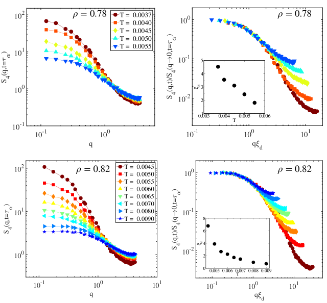
Figure S3: Top Left Panel: Dynamic structure factor $(S_{4}(q,t=\tau_{\alpha}))$ for $\rho=0.78$ as a function of wave vector $(q)$ for different temperature . Top Right Panel: Scaling plot $S_{4}(q,t)/S_{4}(q\to 0,t=\tau_{\alpha})$ vs $q\xi_{d}$ for the 108000 particle simulations. Bottom Panel: Similar plot for $\rho=0.82$. The dynamic length scale as a function of temperature is shown in the inset.

Another important quantity that can provide a lot of the information about dynamic heterogeneity is the four-point correlation function, $g_{4}(r,t)$, and its associated susceptibilities chandan92 defined as,

$$\begin{split}g_{4}(r,t)=\langle\delta\rho(0,0)\delta\rho(0,t)\delta\rho(r,0)\delta\rho(r,t)\rangle-\\ \langle\delta\rho(0,0)\delta\rho(0,t)\rangle\langle\delta\rho(r,0)\delta\rho(r,t)\rangle\end{split}$$ (5)

$\delta\rho(r,t)$ is the deviation of local density $\rho(r,t)$ at position $r$ and time $t$ from its average value $\rho_{0}(r,t)$, $\langle...\rangle$ represents the thermal or time average. The four-point time dependent structure factor $S_{4}(q,t)$ JCP119-14, is related to $g_{4}(r,t)$ via Fourier transformation, as defined below,

$$S_{4}(q,t)=N[\langle Q(q,t)Q(-q,t)\rangle-\langle Q(q,t)\rangle^{2}]$$ (6)

where

$$Q(q,t)=\frac{1}{N}\sum_{i=1}^{N}e^{i\vec{q}.\vec{r}_{i}(0)}w(|\vec{r}_{i}(t)-\vec{r}_{i}(0)|),$$ (7)

The window function $w(x)$ is defined in the same way as it is in Eq. 3. In the small wave vector ($q$) limit, the behavior of $S_{4}(q,t)$ can be described by the Ornstein–Zernike (OZ) form,

$$S_{4}(q,t=\tau_{\alpha})=\frac{S_{4}(q\to 0,t)}{1+(q\xi_{d})^{2}}$$ (8)

in which $\xi_{d}$ is the measure of the length scale that is associated with dynamically correlated region. To access the low wave vector $(q\to 0)$ limit, it is necessary to do large scale simulations. In this study, we measure the dynamics length from system that consists of $N=108000$ particles. In left panel of Fig. S2 and Fig. S3, we plot the $S_{4}(q,t=\tau_{\alpha})$ as a function of wave vector $q$. We fit $S_{4}(q,t)$ to the Ornstein-Zernike (OZ) form in the range $q\xi_{d}\leq 1.0$ to get the dynamic length scale. We did a scaling plot $S_{4}(q,t=\tau_{\alpha})/S_{4}(q\to 0,t=\tau_{\alpha})$ vs $q\xi_{d}$ in the right panel of Fig. S2 and Fig. S3 using the value of $\xi_{d}$ obtained from the OZ fit, and we found a very good scaling collapse for all the different fragile systems. The dynamic length scale is shown as a function of temperature in the insets of all plots.

IV Methods to obtain static length scale

IV.1 Point-to-set method

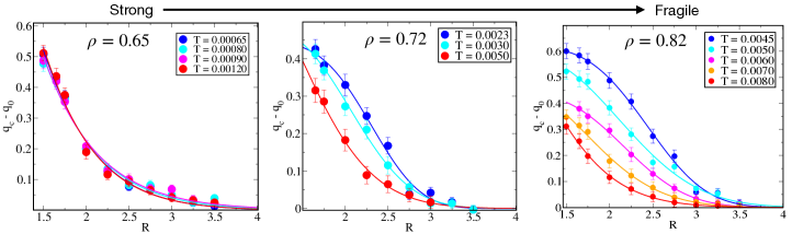
Figure S4: The static overlap as a function of cavity radius $R$ for different temperature. The systems transition from strong to fragile glass (from left to right) with increasing density.

One of the most difficult challenges in glass physics is to determine a growing thermodynamic or structural order that is correlated with the slowing down of dynamics. This becomes much more difficult, when conventional structural features (e.g., pair correlation function) for supercooled liquids and glasses don’t display any noticeable differences from their high temperature liquid states. This problem necessitates a new approach to capturing the elusive thermodynamic order that emerges as the system transitions from liquid to glass while remaining disordered. To calculate the thermodynamic or structural length scale for amorphous systems in an order-agnostic way as envisioned in RFOT theory PhysRevA.40.1045, Bouchaud and Biroli doi:10.1063/1.1796231 suggested a non-trivial correlation known as point-to-set (PTS) correlations Natphy2008. Here, we follow their protocol as given in Ref. Natphy2008 to measure the thermodynamic length scale also referred often as “point-to-set (PTS)” length scale.

We perform NVT molecular dynamics simulations to produce the equilibrium bulk configurations at the desired density and temperature. We then start with the above equilibrium configuration and freeze the particles outside of a cavity of radius $R$, then re-equilibrated the particles within the cavity (called as mobile particles) of radius $R$ in the presence of frozen boundary conditions. A static overlap is established between the original equilibrated configuration and the new equilibrated configuration with the frozen boundary field. To define the static overlap $(q_{c}(R))$, we divide the cavity’s central region into $M$ cubic boxes with side $l$. We select the box size so that there is a negligible chance of having more than one particle in a box. The static overlap is defined as

$$q_{c}(R)=\lim_{t\to\infty}\frac{1}{Ml^{3}\rho}\sum\limits_{i=1}^{M}\langle n_{i}(0)n_{i}(t)\rangle.$$

where $\langle..\rangle$ denotes the both thermodynamic and ensemble average. Here we have chosen $M=125$ cubic boxes of side $l=0.36$. The overlap between two similar configurations is $1$ after normalization and $q_{0}=\rho l^{3}$ for two totally uncorrelated configurations. In Fig. S4 we plot the $q_{c}-q_{0}$ as a function of cavity radius $R$ for various temperatures at a given density. The length scale $(\xi_{pts})$ was calculated using a compressed exponential form to fit the overlap correlation as a function of radius $R$.

$$\tilde{q}(R)=q_{c}(R)-q_{0}=A\exp\left[-\left(\frac{R-a}{\xi_{pts}}\right)^{\eta}\right],$$

We chose $a=1$ because cavities with $R=1$ should only contain a single particle on average, and the overlap properties at this cavity size should not be affected by increasing amorphous order. We have shown the obtained static length scale $(\xi_{s})$ in the main manuscript.

V Static length scale from block statistics of $\tau_{\alpha}$

Figure S5: Top Left Panel: $\chi_{\tau}$ for $\rho=0.65$ as a function of block size $(L_{B})$ for different temperature. Top Right Panel: Scaling collapse to get the static length scale. Bottom Panel: Similar plot for $\rho=0.72$.

In Ref. PhysRevLett.119.205502 an elegant and efficient method for determining the static length scale of the glass forming liquid from the statistics of $\tau^{(i)}_{\alpha}$ on the block size was proposed. We have used the same procedure here. We first calculate the relaxation time ($\tau_{\alpha}^{(i)}(L_{B})$) for each block using the method of Ref. PhysRevLett.119.205502 by measuring the time at which the overlap correlation $(Q^{(i)}(L_{B},t))$ for a given time origin reaches the value $1/e$ (the superscript $i$ indicates that the quantity is collected for a single block prior to any averaging).

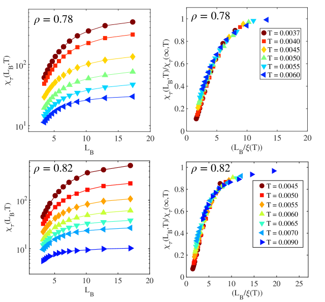
Figure S6: Top Left Panel: $\chi_{\tau}$ for $\rho=0.78$ as a function of block size $(L_{B})$ for different temperature. Top Right Panel: Scaling collapse to get the static length scale. Bottom Panel: Similar plot for $\rho=0.82$.

We measured the mean and variance of the quantity $\tau_{\alpha}^{(i)}(L_{B})$ and define $\chi_{\tau}(L_{B},T)$ as

$$\chi_{\tau}(L_{B},T)=L_{B}^{3}\left\langle\frac{\frac{1}{N_{B}}\sum_{i=1}^{N_{B}}[\Delta\tau_{\alpha}^{(i)}(L_{B})]^{2}}{{[\overline{\tau_{\alpha}^{(i)}(L_{B})}]}^{2}}\right\rangle,$$ (9)

where $\overline{\tau_{\alpha}^{(i)}(L_{B})}=\frac{1}{N_{B}}\sum_{i=1}^{N_{B}}\tau_{\alpha}^{(i)}(L_{B})$, $\Delta\tau_{\alpha}^{(i)}(L_{B})=\tau_{\alpha}^{(i)}(L_{B})-\overline{\tau_{\alpha}^{(i)}(L_{B})}$, and the time-origin averaging is denoted by the outermost angular brackets. This quantity $\chi_{\tau}$ has a strong block size $(L_{B})$ dependence, indicating a growing length scale as temperature decreases. We used scaling analysis to determine the static length scale that can be derived from the scaling collapse of $\chi_{\tau}$. In Fig. S5 and Fig. S6 we plot the $\chi_{\tau}$ as a function of $L_{B}$ and its scaling collapse to obtain the static length scale. In the main paper, a comparison of the static length scale obtained from statistics of $\tau^{(i)}_{\alpha}$ on block size and point-to-set length is shown.

VI STATIC LENGTH SCALE FROM FINITE SIZE SCALING OF $\tau_{\alpha}$

Finally, we also have calculated the static length scale from finite size scaling of $\alpha$-relaxation time $(\tau_{\alpha})$ for the strong liquid following the procedure of Ref. PhysRevE.86.061502. This is mainly done to make sure that the growth of static length scale for strong liquids is weak as obtained using PTS and block analysis methods. In the left panel of Fig. S7 we plot the re-scaled relaxation time (rescaled by asymptotically large system size value of the relaxation time ($\tau_{\alpha}(\infty,T)$) ) for different temperatures and system sizes. In the right panel we show the full data collapse by using the static length scale at different temperatures. The credibility of the obtained static length scale is bolstered by the reasonable data collapse. The static length scale produced from the finite size scaling of $\tau_{\alpha}$, point-to-set method, and statistics of $\tau^{(i)}_{\alpha}$ on block size at different temperatures are compared in the inset and we find that the lengths measured using these various methods are very similar.

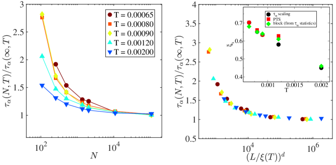
Figure S7: Left Panel: System size dependence of $\alpha$-relaxation time for strong liquid ($\rho=0.65$). Right Panel: Scaling collapse to get the static length scale. Inset: Comparison of the length scales from different methods.

VII Calculation of Onset temperature

We looked at the features of local potential energy minima sampled by the liquid to find a crossover or onset temperature below which the liquid starts to show very sluggish dynamics and thermodynamic and dynamical traits begin to depart from its high temperature liquid sastry_nature,B008749L,sri_Nature. This approach in the field of disordered system is well-known as the energy landscape view or paradigm. To get the inherent state (IS), we performed energy minimization over $1000$ configurations at each temperature and density state point. Inherent states for different fragile liquids are obtained for a wide range of temperatures, from high to very close to the glass transition point. In left y-axis of Fig. S8, we plot the average IS energies ($e_{IS}$, black circles) against each of the studied temperatures for different fragile liquids. The plot shows that for high temperature, the average inherent state energy is nearly temperature independent and begins to show a strong temperature dependence at a certain crossover temperature. The deviation point from the high temperature is taken as the crossover temperature or onset temperature of “slow dynamics” (indicated in each plot by a vertical line). On the right y-axis of Fig. S8 we plot the relaxation time (blue squares) as a function of temperature. We show that the system’s relaxation time begins to increase from the same onset temperature as mined by the inherent state energy analogy. Above the onset temperature, the system relaxes in an exponential manner, similar to a high-temperature liquid. We have used these onset temperatures to scale the data of the temperature dependence of static length scale for a good comparison.

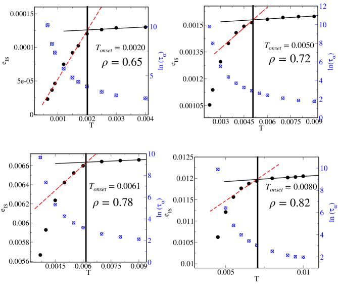
Figure S8: Temperature dependence of the average inherent state energies ($e_{IS}$) shown by black circles in left y-axis for different fragile liquids. System’s relaxation time against temperature are plotted in right y-axis. Onset temperature indicated in each plot by a vertical line.

ieeetr Paper_fragility

References

- (1) L. Berthier, G. Biroli, J.-P. Bouchaud, L. Cipelletti, D. E. Masri, D. L’Hôte, F. Ladieu, and M. Pierno, “Direct experimental evidence of a growing length scale accompanying the glass transition,” Science, vol. 310, no. 5755, pp. 1797–1800, 2005.
- (2) L. Berthier and G. Biroli, “Theoretical perspective on the glass transition and amorphous materials,” Rev. Mod. Phys., vol. 83, pp. 587–645, Jun 2011.
- (3) S. Karmakar, C. Dasgupta, and S. Sastry, “Growing length scales and their relation to timescales in glass-forming liquids,” Annual Review of Condensed Matter Physics, vol. 5, no. 1, pp. 255–284, 2014.
- (4) I. Tah, S. Sengupta, S. Sastry, C. Dasgupta, and S. Karmakar, “Glass transition in supercooled liquids with medium-range crystalline order,” Phys. Rev. Lett., vol. 121, p. 085703, Aug 2018.
- (5) R. Das, I. Tah, and S. Karmakar, “Possible universal relation between short time -relaxation and long time -relaxation in glass-forming liquids,” The Journal of Chemical Physics, vol. 149, no. 2, p. 024501, 2018.
- (6) I. Tah, A. Mutneja, and S. Karmakar, “Understanding slow and heterogeneous dynamics in model supercooled glass-forming liquids,” ACS Omega, vol. 6, pp. 7229–7239, 03 2021.
- (7) C. A. Angell, “Formation of glasses from liquids and biopolymers,” Science, vol. 267, no. 5206, pp. 1924–1935, 1995.
- (8) S. Sastry, P. G. Debenedetti, and F. H. Stillinger, “Signatures of distinct dynamical regimes in the energy landscape of a glass-forming liquid,” Nature, vol. 393, no. 6685, pp. 554–557, 1998.
- (9) L. M. Martinez and C. A. Angell, “A thermodynamic connection to the fragility of glass-forming liquids,” Nature, vol. 410, no. 6829, pp. 663–667, 2001.
- (10) K. Ito, C. T. Moynihan, and C. A. Angell, “Thermodynamic determination of fragility in liquids and a fragile-to-strong liquid transition in water,” Nature, vol. 398, no. 6727, pp. 492–495, 1999.
- (11) P. G. Debenedetti and F. H. Stillinger, “Supercooled liquids and the glass transition,” Nature, vol. 410, no. 6825, pp. 259–267, 2001.
- (12) N. A. Mauro, M. Blodgett, M. L. Johnson, A. J. Vogt, and K. F. Kelton, “A structural signature of liquid fragility,” Nature Communications, vol. 5, no. 1, p. 4616, 2014.
- (13) C. Dalle-Ferrier, A. Kisliuk, L. Hong, G. Carini, G. Carini, G. D’Angelo, C. Alba-Simionesco, V. N. Novikov, and A. P. Sokolov, “Why many polymers are so fragile: A new perspective,” The Journal of Chemical Physics, vol. 145, no. 15, p. 154901, 2016.
- (14) H. VOGEL, “Das temperaturabhangigkeitsgesetz der viskositat von flussigkeiten,” Phys. Z., vol. 22, pp. 645–646, 1921.
- (15) G. S. Fulcher, “Analysis of recent measurements of the viscosity of glasses,” Journal of the American Ceramic Society, vol. 8, no. 6, pp. 339–355, 1925.
- (16) G. Tammann and W. Hesse, “Die abhängigkeit der viscosität von der temperatur bie unterkühlten flüssigkeiten,” Zeitschrift für anorganische und allgemeine Chemie, vol. 156, no. 1, pp. 245–257, 1926.
- (17) J. Mattsson, H. M. Wyss, A. Fernandez-Nieves, K. Miyazaki, Z. Hu, D. R. Reichman, and D. A. Weitz, “Soft colloids make strong glasses,” Nature, vol. 462, no. 7269, pp. 83–86, 2009.
- (18) D. M. Sussman, M. Paoluzzi, M. C. Marchetti, and M. L. Manning, “Anomalous glassy dynamics in simple models of dense biological tissue,” EPL (Europhysics Letters), vol. 121, p. 36001, feb 2018.
- (19) I. Tah, T. A. Sharp, A. J. Liu, and D. M. Sussman, “Quantifying the link between local structure and cellular rearrangements using information in models of biological tissues,” Soft Matter, 2021.
- (20) K. Fox, “Biopreservation. putting proteins under glass,” Science, vol. 267, no. 5206, pp. 1922–1923, 1995.
- (21) Y. ROOS and M. KAREL, “Plasticizing effect of water on thermal behavior and crystallization of amorphous food models,” Journal of Food Science, vol. 56, no. 1, pp. 38–43, 1991.
- (22) M. Mukherjee, J. Mondal, and S. Karmakar, “Role of and relaxations in collapsing dynamics of a polymer chain in supercooled glass-forming liquid,” The Journal of Chemical Physics, vol. 150, no. 11, p. 114503, 2019.
- (23) C. S. O’Hern, S. A. Langer, A. J. Liu, and S. R. Nagel, “Random packings of frictionless particles,” Phys. Rev. Lett., vol. 88, p. 075507, Jan 2002.
- (24) A. J. Liu and S. R. Nagel, “The jamming transition and the marginally jammed solid,” Annual Review of Condensed Matter Physics, vol. 1, no. 1, pp. 347–369, 2010.
- (25) L. Berthier and T. A. Witten, “Compressing nearly hard sphere fluids increases glass fragility,” EPL (Europhysics Letters), vol. 86, p. 10001, apr 2009.
- (26) F. m. c. Sausset, G. Tarjus, and P. Viot, “Tuning the fragility of a glass-forming liquid by curving space,” Phys. Rev. Lett., vol. 101, p. 155701, Oct 2008.
- (27) “See the supplementary materials attached to the paper for more details on our methodology.,”
- (28) T. R. Kirkpatrick, D. Thirumalai, and P. G. Wolynes, “Scaling concepts for the dynamics of viscous liquids near an ideal glassy state,” Phys. Rev. A, vol. 40, pp. 1045–1054, Jul 1989.
- (29) V. Lubchenko and P. G. Wolynes, “Theory of structural glasses and supercooled liquids,” Annual Review of Physical Chemistry, vol. 58, no. 1, pp. 235–266, 2007. PMID: 17067282.
- (30) H. Staley, E. Flenner, and G. Szamel, “Reduced strength and extent of dynamic heterogeneity in a strong glass former as compared to fragile glass formers,” The Journal of Chemical Physics, vol. 143, no. 24, p. 244501, 2015.
- (31) M. D. Ediger, “Spatially heterogeneous dynamics in supercooled liquids,” Annual Review of Physical Chemistry, vol. 51, no. 1, pp. 99–128, 2000. PMID: 11031277.
- (32) N. Lačević, F. W. Starr, T. B. Schrøder, V. N. Novikov, and S. C. Glotzer, “Growing correlation length on cooling below the onset of caging in a simulated glass-forming liquid,” Phys. Rev. E, vol. 66, p. 030101, Sep 2002.
- (33) R. Yamamoto and A. Onuki, “Dynamics of highly supercooled liquids: Heterogeneity, rheology, and diffusion,” Phys. Rev. E, vol. 58, pp. 3515–3529, Sep 1998.
- (34) N. Lačević, F. W. Starr, T. B. Schrøder, and S. C. Glotzer, “Spatially heterogeneous dynamics investigated via a time-dependent four-point density correlation function,” The Journal of Chemical Physics, vol. 119, no. 14, pp. 7372–7387, 2003.
- (35) S. Chakrabarty, I. Tah, S. Karmakar, and C. Dasgupta, “Block analysis for the calculation of dynamic and static length scales in glass-forming liquids,” Phys. Rev. Lett., vol. 119, p. 205502, Nov 2017.
- (36) K. Paul, S. K. Nandi, and S. Karmakar, “Dynamic heterogeneity in active glass-forming liquids is qualitatively different compared to its equilibrium behaviour,” 2021.
- (37) G. Biroli, J.-P. Bouchaud, K. Miyazaki, and D. R. Reichman, “Inhomogeneous mode-coupling theory and growing dynamic length in supercooled liquids,” Phys. Rev. Lett., vol. 97, p. 195701, Nov 2006.
- (38) I. Tah and S. Karmakar, “Signature of dynamical heterogeneity in spatial correlations of particle displacement and its temporal evolution in supercooled liquids,” Phys. Rev. Research, vol. 2, p. 022067, Jun 2020.
- (39) P. Charbonneau, A. Ikeda, J. A. van Meel, and K. Miyazaki, “Numerical and theoretical study of a monodisperse hard-sphere glass former,” Phys. Rev. E, vol. 81, p. 040501, Apr 2010.
- (40) P. Charbonneau, A. Ikeda, G. Parisi, and F. Zamponi, “Dimensional study of the caging order parameter at the glass transition,” Proceedings of the National Academy of Sciences, vol. 109, no. 35, pp. 13939–13943, 2012.
- (41) S. Franz, H. Jacquin, G. Parisi, P. Urbani, and F. Zamponi, “Quantitative field theory of the glass transition,” Proceedings of the National Academy of Sciences, vol. 109, no. 46, pp. 18725–18730, 2012.
- (42) G. Adam and J. H. Gibbs, “On the Temperature Dependence of Cooperative Relaxation Properties in Glass-Forming Liquids,” J. Chem. Phys. , vol. 43, pp. 139–146, July 1965.
- (43) F. m. c. Sausset and D. Levine, “Characterizing order in amorphous systems,” Phys. Rev. Lett., vol. 107, p. 045501, Jul 2011.
- (44) J.-P. Bouchaud and G. Biroli, “On the adam-gibbs-kirkpatrick-thirumalai-wolynes scenario for the viscosity increase in glasses,” The Journal of Chemical Physics, vol. 121, no. 15, pp. 7347–7354, 2004.
- (45) G. Biroli, J. P. Bouchaud, A. Cavagna, T. S. Grigera, and P. Verrocchio, “Thermodynamic signature of growing amorphous order in glass-forming liquids,” Nature Physics, vol. 4, no. 10, pp. 771–775, 2008.
- (46) G. M. Hocky, T. E. Markland, and D. R. Reichman, “Growing point-to-set length scale correlates with growing relaxation times in model supercooled liquids,” Phys. Rev. Lett., vol. 108, p. 225506, Jun 2012.
- (47) K. Hima Nagamanasa, S. Gokhale, A. K. Sood, and R. Ganapathy, “Direct measurements of growing amorphous order and non-monotonic dynamic correlations in a colloidal glass-former,” Nature Physics, vol. 11, no. 5, pp. 403–408, 2015.
- (48) S. Yaida, L. Berthier, P. Charbonneau, and G. Tarjus, “Point-to-set lengths, local structure, and glassiness,” Phys. Rev. E, vol. 94, p. 032605, Sep 2016.
- (49) S. Sastry, “Onset temperature of slow dynamics in glass forming liquids,” PhysChemComm, vol. 3, pp. 79–83, 2000.
- (50) D. Coslovich and G. Pastore, “Understanding fragility in supercooled lennard-jones mixtures. i. locally preferred structures,” The Journal of Chemical Physics, vol. 127, no. 12, p. 124504, 2007.
- (51) J. E. Hallett, F. Turci, and C. P. Royall, “Local structure in deeply supercooled liquids exhibits growing lengthscales and dynamical correlations,” Nature Communications, vol. 9, no. 1, p. 3272, 2018.
- (52) H. Tong and H. Tanaka, “Revealing hidden structural order controlling both fast and slow glassy dynamics in supercooled liquids,” Phys. Rev. X, vol. 8, p. 011041, Mar 2018.
- (53) J. Mattsson, H. M. Wyss, A. Fernandez-Nieves, K. Miyazaki, Z. Hu, D. R. Reichman, and D. A. Weitz, “Soft colloids make strong glasses,” Nature, vol. 462, no. 7269, pp. 83–86, 2009.
- (54) J. Towns, T. Cockerill, M. Dahan, I. Foster, K. Gaither, A. Grimshaw, V. Hazlewood, S. Lathrop, D. Lifka, G. D. Peterson, R. Roskies, J. R. Scott, and N. Wilkins-Diehr, “Xsede: Accelerating scientific discovery,” Computing in Science & Engineering, vol. 16, pp. 62–74, Sept.-Oct. 2014.
- (55) W. Kauzmann, “The nature of the glassy state and the behavior of liquids at low temperatures.,” Chemical Reviews, vol. 43, pp. 219–256, 10 1948.
- (56) S. P. Das, “Mode-coupling theory and the glass transition in supercooled liquids,” Rev. Mod. Phys., vol. 76, pp. 785–851, Oct 2004.
- (57) W. Gotze, Complex dynamics of glass-forming liquids : a mode-coupling theory. Oxford: Oxford University Press, 2009.
- (58) C. Dasgupta, V. A. Indrani, S. Ramaswamy, and K. M. Phani, “Is there a growing correlation length near the glass transition?,” Europhys. Lett., vol. 15, pp. 307–312, June 1991.
- (59) N. Lacevic, W. F. Star, B. T. Schroder, and C. S. Glotzer, “Spatially heterogeneous dynamics investigated via a time-dependent four-point density correlation function,” The Journal of Chemical Physics, vol. 119, pp. 7372–7387, Jan 2003.
- (60) S. Karmakar and I. Procaccia, “Finite-size scaling for the glass transition: The role of a static length scale,” Phys. Rev. E, vol. 86, p. 061502, Dec 2012.
- (61) S. Sastry, “The relationship between fragility, configurational entropy and the potential energy landscape of glass-forming liquids,” Nature, vol. 409, no. 6817, pp. 164–167, 2001.