Human-In-The-Loop Document Layout Analysis

Abstract

Document layout analysis (DLA) aims to divide a document image into different types of regions. DLA plays an important role in the document content understanding and information extraction systems. Exploring a method that can use less data for effective training contributes to the development of DLA. We consider a Human-in-the-loop (HITL) collaborative intelligence in the DLA. Our approach was inspired by the fact that the HITL push the model to learn from the unknown problems by adding a small amount of data based on knowledge. The HITL select key samples by using confidence. However, using confidence to find key samples is not suitable for DLA tasks. We propose the Key Samples Selection (KSS) method to find key samples in high-level tasks (semantic segmentation) more accurately through agent collaboration, effectively reducing costs. Once selected, these key samples are passed to human beings for active labeling, then the model will be updated with the labeled samples. Hence, we revisited the learning system from reinforcement learning and designed a sample-based agent update strategy, which effectively improves the agent’s ability to accept new samples. It achieves significant improvement results in two benchmarks (DSSE-200 (from 77.1% to 86.3%) and CS-150 (from 88.0% to 95.6%)) by using 10% of labeled data.

Index Terms—  Human-in-the-loop, key samples, agent collaboration, document layout analysis, deep learning.

1 Introduction

The Document Layout Analysis (DLA) is an important task dedicated to extracting semantic information from the document image. As a critical preprocessing step of document understanding systems, DLA can provide information for several applications such as document retrieval, content categorization, and text recognition. With the development of deep convolutional neural networks, the high-capacity supervised learning algorithms have achieved remarkable results in DLA tasks [1, 2, 3, 4, 5, 6]. The scale of these models has included hundreds of millions of parameters. This paradigm allows the model to have more degrees of freedom enough to awe-inspiring description power. However, the large number of parameters requires a massive amount of training data with labels [7]. Improving model performance by data annotation has two crucial challenges. On the one hand, the data growth rate is far behind the growth rate of model parameters, so data growth has primarily hindered the further development of the model. On the other hand, the emergence of new tasks has far exceeded the speed of data updates. Suppose you have developed an industrial model for defect detection. If the production line needs to adjust short-term production goals, you have to label new data and train the model. The time of data annotation will become the bottleneck of the application.

Many tasks generate samples to construct new datasets, thereby speeding up model iteration and reducing the cost of data annotation [8, 9, 10, 11]. However, the generated data cannot fully satisfy the intricate details in the task, and the quality of the generated data is difficult to be effectively guaranteed. For DLA tasks, some samples in the different datasets are similar. If we can accurately find and label the key samples, our model can learn Knowledge better and reduce data annotation pressure. The central issue addressed in this paper is the following: How we find the key samples on the new dataset that do not exist in the original dataset?

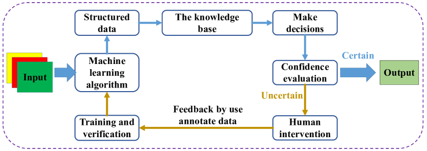
Fig. 1: A Human-in-the-loop Machine Learning Pipeline.

To tackle this challenge, the Human-in-the-loop (HITL) methods are proposed [12, 13, 14], and the pipeline shown in Fig. 1. HITL uses each sample’s confidence to judge whether the key samples. The use of confidence to find key samples is a milestone in the classification task. However, confidence cannot be directly obtained in some tasks, the confidence’s magic is not attractive. For example, the segmentation task is a pixel-level classification, confidence cannot be used to find the key samples, so we need to explore a way to find the key samples. When people explore unknown problems, they usually need necessary discussions. First, different people will make necessary inferences based on their knowledge; then put forward their thinking about this problem; finally, they discuss and use the discussion’s consensus to define this problem. So, we propose a framework for multi-agent collaboration under the framework of HITL.

This framework’s motivation is to consider that when people learn about unknown problems, they always reason based on existing knowledge and only need a few key pieces of information to update knowledge. Our framework consists of three parts, the agent initialization, the agent collaboration, and the agent update. (1) Agent initialization: the agent should know more scenes and things, but it is unnecessary for detailed information in the domain. This process may be similar to most models’ current training using ImageNet, which means we need to use more data to train our initial model. These data do not require a perfect fit with the target task. Maybe it is related domain data or machine-synthesized data, as long as the amount of data is huge. Inspired by data generation, we train the initial model by using generate some initial data. We design a sample synthesis engine base on LaTex to synthesize a large amount of data as the initial knowledge carrier. We will describe the specific synthesis process in section 3.1. (2) Agent collaboration: agent collaboration is to discover the key samples. Most samples in the new dataset are similar to the original dataset, the data difference only depends on a few samples. In this process, We use two pre-trained models to deal with the unlabeled data to obtain forecast results, and then we compare the pixel classification results of the two output results. Finally, we get the samples by filter threshold. (3) Agent update: the agent update uses human-labeled data to train the agent to learn new knowledge. Follow the reinforcement learning, and we will consider an update method that distinguishes the sample distribution.

This paper mainly makes three contributions:

• We propose a multi-agent collaboration framework under the Human-in-the-loop that can accurately discover key sample using as few human efforts as possible. To the best of our knowledge, we are the first to propose the framework for agent collaboration under the HITL.

• We propose a key samples method that can more accurately find key samples in high-level tasks (semantic segmentation) through agent collaboration, thus effectively reducing the human efforts.

• We design a sample-based agent update strategy, which effectively improves the agent’s ability to accept new samples.

• We apply our framework to the DSSE-200 [15] and CS-150 [16] DLA datasets and find that it outperforms the state-of-the-art approaches.

The rest of this paper is organized as follows. Section 2 introduces background of document layout analysis and Human-in-the-loop. Section 3 discusses the model design and network architecture in detail. In Section 4, we demonstrate the qualitative and quantitative study of the framework. Finally, we conclude our work in Section 5.

2 Related Works

2.1 Document Layout Analysis

Document layout analysis (DLA) methods can be divided into three categories known as bottom-up, top-down, and hybrid. The bottom-up strategy can be subdivided into five categories, and the representative work has the following: specifically connected component analysis [17], texture analysis [18], learning-based analysis, Voronoi diagram [19], and Delaunay triangulation [20]. The top-down strategy can be subdivided into four categories. The representative work has the following: texture-based Analysis [21], Run Length Smearing Algorithm (RLSA) [22], DLA projection-profile [23] and White space analysis [24]. The hybrid methods offer a balance between bottom-up and top-down techniques. Chen et al. [25] propose an effective hybrid method for page segmentation, which extracts blank rectangles based on connected component analysis, and uses foreground and background information to filter blank rectangles to form new separators. Many researchers use multi-level homogeneity structure (MHS) for document layout analysis [26, 27]. Besides, many methods based on neural networks [2, 3, 4, 5, 6] have been proposed and achieved remarkable results. Rencently, the DLA task can also be considered as a semantic segmentation task, which is to perform a pixel-level understanding of the segmentation object [28, 29, 30]. Xu et al. [31] train a multi-task FCN to segment the document image into different regions. Soullard et al. [32] propose a fully convolutional neural network architecture (FCN) to deal with historical newspaper images by using a pixel labelling of the various semantic entities. Zheng et al. [33] propose a deep generative model for graphic design layouts to synthesize layout designs. Zheng et al. [34] propose a novel cross-domain DOD model to learn a detector for the target domain using labelled data from the source domain and only unlabeled data from the target domain. Xu et al. [35] propose the LayoutLM to jointly model interactions between text and layout information across scanned document images. Many of these papers employ the Fully Convolutional Network (FCN, [36]) for semantic segmentation.

As pointed out by Binmakhashen et al. [1] in their survey, the deep-learning DLA methods require a long training time and huge data. Therefore, exploring a method that can use less data for effective training contributes to the development of document layout.

2.2 Human-In-The-Loop

Active Learning Active learning is a commonly used technique in machine learning which involves humans labeling the most interesting examples iteratively  [37, 38]. Active learning has many excellent jobs, such as Uncertainty sampling, Query-by-committee (QBC), Expected model change, Expected error reduction, and Expected error reduction [39]. However, the agents in these algorithms cannot try to optimize external rewards, and therefore the challenges involved in combining autonomous reinforcement learning with human expertise not be tackled [40]. Our agent collaboration is inspired by QBC [41, 42, 43, 44, 45, 46]. However, there are two differences between KSS and QBC. One is that our labeled samples use a data generation method that does not require manual labeling, and the other is that our agents try to optimize external rewards. Besides, as far as we know, this is the first work to introduce agent collaboration into HITL.

Human-In-The-Loop With the development of convolutional neural networks, the growth rate of model capacity has far exceeded the available data development scale. To enable the model to quickly learn to ‘solve’ a new task by giving it a few training examples of a new task, some few-shot learning approaches have been proposed [47, 48]. To allow the network to effectively learn novel categories from only a few training data while at the same time it will not forget the initial categories, Gidaris et al. designed a few-shot visual learning system [49]. Yao et al. proposed a graph few-shot learning (GFL) algorithm, which shares a transferable metric space characterized by node embedding and graph-specific prototype embedding functions between the auxiliary graph the target, thereby promoting the transfer of structural knowledge. GFL learns prior knowledge from the auxiliary graph to improve the classification accuracy of the target graph [50]. The well-known network structure of meta-learning also includes Siamese neural network [51], matching network [52] and prototype network [53].

Many generate-based methods can also expand the size of the dataset well. In particular, the method of using Generative Adversarial Networks (GAN) [54] has achieved state-of-the-art performance on many tasks [55]. To make better use of the image generator’s semantic layout, Liu et al. [10] used a convolution kernel conditioned on the semantic label map to generate an intermediate feature map from the noise map and finally generated an image. Liu et al. [9] proposed a novel LayoutGAN to generate the layout of relational graphic elements.

HITL selects the most useful samples to improve conventional machine learning tasks’ performance has become a hot topic in recent research. Li et al.[56] proposed a hybrid human-machine data integration framework for data integration problems that purely automated methods cannot completely address. In response to the lack of data samples in current learning methods, Maxime et al.[57] used the HITL method to develop a platform named BabyAI to support investigations towards including humans in the loop for grounded language learning. To address the challenge that deep learning needs to rely on a large amount of manually labeled data, Zhang et al.[14] proposed a framework that combines the advantages of regular expressions and deep learning. Many tasks have almost no annotated data and always need to be created from scratch. To address this challenge, Klie et al.[58] proposed a novel domain-agnostic HITL annotation approach. Yue et al.[13] proposed a framework named Interventional Few-Shot Learning (IFSL) to address an overlooked deficiency in recent FSL methods. Wan et al.[12] proposed a HILL learning algorithm to dynamically reject uncertain predictions and mark them to increase a novel set of categories.

The above methods are largely considered to deal with the lack of data, and they are all excellent work. However, these methods have certain limitations in finding error-prone samples. Therefore, we propose an agent collaboration method to select key samples.

3 Approach

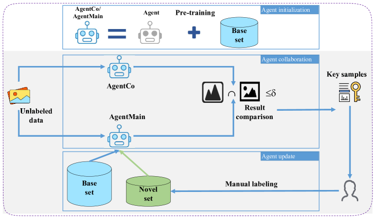
Fig. 2: The architecture of our framework. It consists of three parts: agent initialization, agent collaboration and agent update.

As shown in Fig. 2, our framework consists of three parts: agent initialization, agent collaboration, and agent update. First, we generate a large-scale sample ($D_{base}$) using a sample synthesis engine base on LaTex. Then we use the large-scale datasets to train two general agent models. Next, we use unlabeled samples ($D_{novel}$) as input prediction results using two agents, and we compare the two prediction results to obtain a key sample with large prediction differences. Finally, we make manual labeling these key samples and use them as input to retrain the model.

We assume there are $K_{base}$ base samples, and there are $N_{b}$ categories:

$${D_{base}}=\bigcup\limits_{b=1}^{{K_{base}}}{\left\{{{x_{b}},i}\right\}}_{i=1}^{{N_{b}}}$$ (1)

Where $K_{base}$ is the number of base samples, ${x_{b}},i$ is the $i-th$ sample in base samples b that is composed of $N_{b}$ class. Similarly, we can define the novel set as Eq. 2

$${D_{novel}}=\bigcup\limits_{n=1}^{{K_{novel}}}{\left\{{{x_{n}},i}\right\}}_{i=1}^{{N_{n}}}$$ (2)

The agent initialization is to establish a general model. To briefly describe this process, we use $f(.)$ to represent the main agent model’s training process and use $g(.)$ to represent the training process of the collaborative agent model. we define the ${x_{m}}\in{\mathbb{R}^{m}}=f({\hat{x}_{b}})$ as the feature vector extracted from the base data ${\hat{x}_{b}}({\hat{x}_{b}}\in{D_{base}})$ via function $f(.)$, we can get a training weight set as $W_{m}^{*}=\bigcup\nolimits_{m=1}^{{N_{b}}}{\left\{{\omega_{m}^{*}}\right\}}$. Similarly, we define the ${x_{c}}\in{\mathbb{R}^{m}}=f({\hat{x}_{b}})$ as the feature vector extracted from the base data ${\hat{x}_{b}}({\hat{x}_{b}}\in{D_{base}})$ via function $g(.)$, we can get a training weight set as $W_{c}^{*}=\bigcup\nolimits_{c=1}^{{N_{b}}}{\left\{{\omega_{c}^{*}}\right\}}$.

The agent collaboration is to select key samples, input the new sample into the trained agent, compare the results’ intersection, and select the key samples in the two agents. We can get the output of the main agent model as Eq. 3, and the output of the collaborative agent model as Eq. 4.

$${O^{m}}({\hat{x}_{n}})=\delta({\tau_{m}}\cdot{x_{m}}\cdot{\omega_{m}}\cdot{\hat{x}_{n}})$$ (3)

$${O^{c}}({{\hat{x}}_{n}})=\delta({\tau_{c}}\cdot{x_{c}}\cdot{\omega_{c}}\cdot{{\hat{x}}_{n}})$$ (4)

Where $\delta(.)$ is a post-processing operation, and its function is to map the final feature matrix through operations such as softmax to obtain the most likely classification result matrix. ${\hat{x}_{b}}$ from the novel data ${\hat{x}_{n}}({\hat{x}_{n}}\in{D_{novel}})$, $\tau_{m}$ and $\tau_{c}$ are learnable parameter. By solving the number of intersections of the two samples’ results, we can help us get the key samples. Assume $\hat{x}$ is a matrix size is $w\times h$, and $SC(.)$ is used as a scaling factor, the size of the output matrix of the agent is $SC(w)\times SC(h)$. We can define the score of the key samples as Eq. 6.

$${ScoreK({{\hat{x}}_{n}})={O^{m}}({{\hat{x}}_{n}})\cap{O^{c}}({{\hat{x}}_{n}})}$$ (5)

$$ScoreK({\hat{x}_{n}})=\frac{{\sum\limits_{i=1}^{SC(w)}{\sum\limits_{j=1}^{SC(h)}{(\left[{O_{ij}^{m}=O_{ij}^{m}}\right])}}}}{{SC(w)\times SC(h)}}$$ (6)

Key 1: (Validation of Key Samples Selection) The previous HITL framework did not consider processing pixel-level classification, so there is no formed sample selection strategy. Here we set three confidence scoring strategies (Eq. 7, Eq. 8, Eq. 9) based on the usual confidence selection algorithm, and cooperate with our multi-agent strategy comparison. We assume that the final output feature is $F_{whd}$, $w$ represents the feature width at this time, $h$ represents the feature height, and $d$ represents the number of feature channel layers. At this time, $d$ and the number of classifications are the same as $N_{b}$.

$$MACON:\left\{{\begin{array}[]{*{20}{c}}{f_{ij}^{1}=\frac{1}{{1+{e^{-\max\{{F_{ijk}}\}_{k=1}^{d}}}}}}\\ {co{n_{1}}=\frac{{\sum\limits_{i=1}^{w}{\sum\limits_{j=1}^{h}{\left({{{f_{ij}^{1}}\mathord{\left/{\vphantom{{f_{ij}^{1}}{\sum{{f^{1}}}}}}\right.\kern-1.2pt}{\sum{{f^{1}}}}}}\right)}}}}{{w\times h}}}\end{array}}\right.$$ (7)

$$SUCON:\left\{{\begin{array}[]{*{20}{c}}{f_{ij}^{2}=\frac{1}{{1+{e^{-sum\{{F_{ijk}}\}_{k=1}^{d}}}}}}\\ {co{n_{2}}=\frac{{\sum\limits_{i=1}^{w}{\sum\limits_{j=1}^{h}{\left({{{f_{ij}^{2}}\mathord{\left/{\vphantom{{f_{ij}^{2}}{\sum{{f^{2}}}}}}\right.\kern-1.2pt}{\sum{{f^{2}}}}}}\right)}}}}{{w\times h}}}\end{array}}\right.$$ (8)

$$MECON:\left\{{\begin{array}[]{*{20}{c}}{f_{ij}^{3}=\frac{1}{{1+{e^{-median\{{F_{ijk}}\}_{k=1}^{d}}}}}}\\ {co{n_{3}}=\frac{{\sum\limits_{i=1}^{w}{\sum\limits_{j=1}^{h}{\left({{{f_{ij}^{3}}\mathord{\left/{\vphantom{{f_{ij}^{3}}{\sum{{f^{3}}}}}}\right.\kern-1.2pt}{\sum{{f^{3}}}}}}\right)}}}}{{w\times h}}}\end{array}}\right.$$ (9)

We will verify the method effect in the section 4.5.

The agent update is to use new samples to train the model so that the model’s ability to recognize unknown samples can be effectively enhanced. This process can be expressed as Eq. 10.

$$\omega_{m}^{*}\leftarrow\gamma(D_{key})$$ (10)

Where $\gamma(.)$ is a retrain operation, $D_{key}$ is a mixed dataset, we will explain in detail next.

Key 2: (Validation of Agent Update) We try to directly use select examples for fine-tuning (Eq. 12), use select data plus original data for fine-tuning (Eq. 13), use mix data to retrain the model (Eq. 14), and use reinforcement learning for training (Eq. 15). Since the number of select samples is very limited, we will crop new sample images, tables, and text resources to prevent the agent from falling into overfitting. Moreover, at the same time, select some materials from the original material library and use a sample synthesis engine base on LaTex to automatically expand a part of the data ($D_{synthesis}$), and then select samples and synthetic data to form a new training sample ($D^{\prime}_{novel}$). The process is shown in Eq. 11.

$${D^{\prime}_{novel}}={D_{novel}}\cup{D_{synthesis}}$$ (11)

$$PSFT:\left\{{\begin{array}[]{*{20}{c}}{\omega_{m}^{*}\leftarrow\omega_{m}^{*}\otimes\gamma(D_{key})}\\ {(D_{key}\not\subset{D_{base}})\cap(D_{key}\subset{D^{\prime}_{novel}})}\end{array}}\right.$$ (12)

$$PBSFT:\left\{{\begin{array}[]{*{20}{c}}{\omega_{m}^{*}\leftarrow\omega_{m}^{*}\otimes\gamma(D_{key})}\\ {(D_{key}\subset{D_{base}})\cup(D_{key}\subset{D^{\prime}_{novel}})}\end{array}}\right.$$ (13)

$$RBSFT:\left\{{\begin{array}[]{*{20}{c}}{\omega_{m}^{*}\leftarrow\gamma(D_{key})}\\ {(D_{key}\subset{D_{base}})\cup(D_{key}\subset{D^{\prime}_{novel}})}\end{array}}\right.$$ (14)

$$RBSRE:\left\{{\begin{array}[]{*{20}{c}}{\omega_{m}^{*}\leftarrow\omega_{m}^{*}\otimes({\lambda_{1}}*\gamma({D_{hb}})+{\lambda_{2}}*\gamma({D_{hn}}))}\\ {{D_{hb}}\Rightarrow D_{key}\subset{D_{base}}}\\ {{D_{hn}}\Rightarrow D_{key}\subset{D^{\prime}_{novel}}}\end{array}}\right.$$ (15)

where $\otimes$ represent the weight update, ${{\lambda_{1}}}$ and ${{\lambda_{2}}}$ are hyperparameters, we will implement them in the next experiment.

3.1 Agent Initialization

The purpose of agent initialization is to establish a general model, the general model can learn the prior knowledge from the original data. The model’s performance is positively correlated with the number of parameters, and the situation that the model with more parameters can handle is more complicated. However, more parameters mean that more samples are needed for parameter constraints. Therefore, the prerequisite for building a general model is to have a sufficient sample to train. There is currently very limited manual labeling data in the DLA field to the best of our knowledge, so we need to find an unlabeled method that can quickly construct data samples. Inspired by the work of Yang et al. [15], we design a sample synthesis engine base on LaTex.

The idea of the generation process is shown in Algorithm 1. The specific process can be similar to playing a jigsaw puzzle in the document. Different from Yang et al., we added more details. The caption also includes a complex font besides different sizes. So we have also collected a title library with screenshots besides simply changing the font size. That will contain many unforeseen deviations using Wikipedia as a source of text, the novel texts published on the Internet as the data source to improve text quality. Besides, our data sources are from network resources, but more of them are collected and intercepted manually by our organization, and the quality is more guaranteed. The number of data sources is also rich enough. In addition to using MSCOCO [59] directly, we also grabbed nearly 20,000 images on the Internet and manually collected 5,000 images from the magazines and web pages.

We generated 3000 samples use the LaTex synthesis engine, and we divided the training set and the validation set with a ratio of 8: 2. The sample layout generated is relatively simple. To not cause excessive dependence on the datasets, we limited the accuracy to below 95% during pre-training.

Input: $PageNumber$ : The number of document,

$Set$ : The attribute of the generated document ;

Output: $Document$ : Generated document,

$label$ : The Ground-True;

1

2for $i=1;i\leq PageNumber$ do

3      

4      Randomly set the font size, randomly set the margins, and randomly set whether to double-column

5      

6      while The remaining page height is not 0 do

7             Randomly select the generation type, and calculate the page remaining according to different types.

8      

9

10return $Document,label$;

11

Algorithm 1 The Exapmple Generation

3.2 Agent Collaboration

We trained two general-purpose agents by using the generated data. The next is to use these two trained agents to collaborate to identify key data. We discovered the fact in the migration learning experiment that the migrated model can already handle most of the data for new datasets, so we need supplementation or human intervention only a few. However, if all the results have to be manually filtered, labor costs will be more expensive. We propose to use two models with different structures for identifying key data. Moreover, in section 4.5, we will verify the effect of using two models with different structures for identifying key data.

Main agent. As shown in Fig. 3, our main agent uses the classic encoder-decoder structure, which has achieved remarkable results in semantic segmentation tasks. The backbone of the encoder uses ResNet18 [60], and we use the spatial pyramid pool proposed in Deeplabv3+ [61] to enhance the features of the encoder output.

It is worth mentioning that, to use high-dimensional semantic information more effectively, we innovatively propose a dynamic residual feature fusion module (DRF), which considers the use of residual structure to maintain category semantic information. As shown in Fig. 3, our DRF first concatenates low-dimensional information with high-dimensional semantic information. Then uses a $3\times 3$ convolutional layer to reduce some channels, and finally, merges high-dimensional information with low-dimensional information. We use deep separable convolution [62] to make the model more efficient. To extract effective weights from high-dimensional features, we use global pooling to process the feature channels first, and then use two batched $1\times 1$ convolutional layers to process the results, and finally use sigmoid for activation.

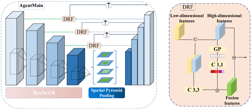
Fig. 3: The structure of Main agent.

Collaborative agent. As shown in Fig. 4, our collaborative agent uses the FCN8 [36] model, which uses a fully convolutional neural network, and the encoder uses VGG16 [63] as the backbone. We use two trained agents to deal with unlabeled data, and then each agent will have different prediction results. The DLA task is essentially a pixel-level classification, the pixel classification results of the two prediction results. We will select a part of the data whose difference is more significant than 25% and mark it manually. This comparison difference is an empirical value.

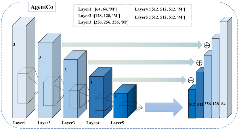
Fig. 4: The structure of cooperative agent.

3.3 Agent Update

The purpose of agent update is to allow the agent to learn unknown knowledge from new samples. Currently, it is mostly achieved by fine-tuning the model. We designed four fine-tuning strategies for this and compared them. The first is to directly use key samples to fine-tune the model, the second considers the use of key samples and initial samples for mixed fine-tuning, and the third considers the use of key samples and initial sample re-tuning. The fourth considers the distribution gap between the new data and the original data. We follow the idea of reinforcement learning and assign new weights to selected samples and basic data (Eq. 15) to make full use of the data. As shown in Eq. 15, ${{\lambda_{1}}}$ and ${{\lambda_{2}}}$ are two hyperparameters that directly act on the loss function. By the experiment, we have determined that the value of ${{\lambda_{1}}}$ is 0.2 and the value of ${{\lambda_{2}}}$ is 0.8. This model can achieve the best effect. We will further prove our update method’s effect in section  4.5.

4 Experiments

Following the setting of the paper [15, 64, 65, 66], we evaluate our model using accuracy, precision, recall and F1 as metrics.

Metric. Several metrics are used to evaluate the performance. We first define $M$ as the $n\times n$ confusion matrix with $n$ categories. Accuracy (Acc) is the ratio of the pixels that are correctly predicted in a given image, i.e.,

$$Acc=\frac{{\sum\nolimits_{i}{{M_{ii}}}}}{{\sum\nolimits_{ij}{{M_{ij}}}}}$$ (16)

Precision (P) is the ratio that is actually a positive example in the example that is divided into positive examples, i.e.,

$$P=\frac{1}{n}\sum\limits_{i=1}^{n}{{P_{i}}}\qquad{P_{i}}=\frac{{{M_{ii}}}}{{\sum\nolimits_{j}{{M_{ji}}}}}$$ (17)

Recall (R) measures the coverage. There are multiple positive examples of metrics that are divided into positive examples, i.e.,

$$R=\frac{1}{n}\sum\limits_{i=1}^{n}{{R_{i}}}\qquad{R_{i}}=\frac{{{M_{ii}}}}{{\sum\nolimits_{j}{{M_{ij}}}}}$$ (18)

$F_{1}$ is an indicator used to measure the accuracy of a binary model. It also takes into account the accuracy and recall rate of the classification model. The $F_{1}$ score can be seen as a weighted average of model accuracy and recall:

$${F_{1}}=\frac{{2\cdot P\cdot R}}{{P+R}}$$ (19)

4.1 Datasets

DSSE-200. The DSSE-200 [15] is a comprehensive dataset, which comes from magazine screenshots, PPT screenshots, book cover screenshots, and old newspapers. It contains 200 images, including seven categories.

CS-150. Clark  et al. proposed the CS-150 [16], it consists of 150 papers and includes 1175 images. The classification criteria in this dataset are divided into three types: image, table, and others.

4.2 Implementation Details

DSSE-200. First, we train AgentCo and AgentMain by using synthetic samples. We split the training set and validation set into 8: 2. Because the generated sample layout is not complicated enough, to prevent over-fitting, we constrain F1 below 95%. Then we use AgentCo and AgentMain to deal with the image of DSSE-200 and obtain pixel classification results of all images, and then we compare the prediction results of the two agents for the same image, find some images with an error rate of more than 25%. For the DSSE-200, we found 23 images, we manually mark these images. Besides, we extracted the materials in these images, and then randomly selected some resources from the resource library, finally put them into our document synthesis tool to generate some samples. Finally, we synthesize 77 images and use the new 100 images to continue to retrain the agent.

CS-150. The CS-150 is relatively simple, and it is composed of simple paper layouts. Therefore, the result is better processed. We limit the samples with a different rate of more than 5% on the first page to obtain 9 images. These 9 images were manually marked. Besides, we extracted the materials in these images, and then randomly selected some resources from the resource library, finally put them into our document synthesis tool to generate some samples. Finally, we synthesize 91 images and use the new 100 images to continue training the model.

Table 1: F1 scores (%) for page segmentation on the datasets. The Baseline means a migration model that is not trained on the new dataset.

Method	DSSE-200				CS-150
	A	P	R	F1	A	P	R	F1
Baseline	80.6	77.9	76.3	77.1	92.9	87.6	88.5	88.0
KSS	86.2	85.1	87.5	86.3	98.5	96.2	95.1	95.6

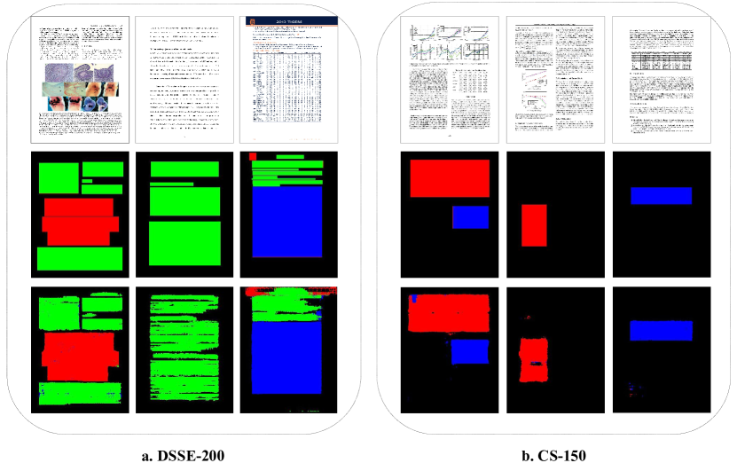
Fig. 5: Example real documents and their corresponding segmentation of DSSE-200 and CS-150. Top: original. Middle: ground-truth. Bottom:predictions. Segmentation label colors are: figure, table, text and background (The CS-150 mark uses text as background).

4.3 Results and Comparisons

DSSE-200. To get fair results, we remove the key samples as a test set. So, the DSSE-200 test set contains 177 images. We obtain the results as shown in Table 1, and we deal with the visualization results as shown in Fig. 5. The baseline model trained with generated data. As shown in Table 1, we used 23 labeled data to improve the performance by 9.2%, so we can see that our method has a certain effect, and we will compare it with randomly selected samples later.

CS-150. The results we got are shown in Table 1, and the visualization results drawn are shown in Fig. 5. As shown in Table 1, we used 23 types of labeled data to increase the performance of the datasets by 7.6%.

4.4 Comparisons with State-ot-the-arts

Table 2: F1 scores (%) for page segmentation on the CS-150 dataset compare with state-of-the-arts.

Method	figure			table
	$P$	$R$	$F_{1}$	$P$	$R$	$F1$
PDFPlots [71]	0.624	0.500	0.555	0.429	0.363	0.393
PDFFigures [16]	0.961	0.911	0.935	0.962	0.921	0.941
PDFFigures 2.0 [67]	0.980	0.961	0.970	0.979	0.963	0.971
KSS	0.984	0.971	0.977	0.978	0.972	0.974

Due to the differences in page classification granularity requirements, DLA tasks also have large differences in page elements’ division. We selected the previous two representative classification methods and compared them. Following the setting of the paper [15], we have an experiment on the DSSE-200. The experiment shows the following Table 3 and Table 4. As can be seen from Table 3 and Table 4, whether it is fine-grained classification or coarse-grained classification, our method is the most effective. Following the setting of the paper [67], we test and compare the CS-150. The results are shown in Table  2. Observing the experimental results in Table 2, our results reached the state-of-the-art.

Table 3: IoU scores (%) for fine-grained page segmentation on the DSSE-200 dataset compare with state-of-the-arts. BG means background.

Method	BG	figure	table	section	caption	list	para.	mean
MFCN [15]	83.9	83.7	79.7	59.4	61.1	68.4	79.3	73.3
KSS	82.2	84.9	82.6	72.5	67.5	75.1	84.3	78.3

Table 4: IoU scores (%) for coarse-grained page segmentation on the DSSE-200 dataset compare with state-of-the-arts.

Methods	no-text	text
Leptonica  [68]	84.7	86.8
Bukhari et al. [69]	90.6	90.3
MFCN (binary) [15]	94.5	91.0
KSS (binary)	96.4	93.2
Methods	figure	text
Fernandez et al. [70]	70.1	85.8
MFCN (binary) [15]	77.1	91.0
KSS (binary)	82.6	91.2

In order to get a fair comparison, we recode several current more competitive structures and compared them with our proposed structure. Because the DSSE-200 and CS-150 do not provide standard training datasets, we randomly select some images as the train data and others as test data. We split DSSE-200 and CS-150 into the training set and test set according to 6:4. We compared the model performance on the DSSE-200 and CS-150 datasets using the conventional training mode, and the results are shown in Table 5. It can be seen from Table 5 that KSS has outstanding performance.

Table 5: F1 scores (%) for page segmentation on dataset. The Para represents the trainable parameter amount of the model, the ’M’ means million.

Method	DSSE-200				CS-150				Para
	A	P	R	F1	A	P	R	F1	(M)
Segnet [72]	83.6	81.8	82.6	82.2	99.3	93.6	93.9	93.7	29
PSPnet [73]	84.6	83.5	84.1	83.8	99.4	93.9	93.3	93.6	46
PANet [74]	81.1	82.6	85.2	83.9	99.2	93.7	94.0	93.8	168
KSS	85.9	82.5	86.3	84.4	99.4	94.5	94.7	94.6	15

4.5 Ablation Study

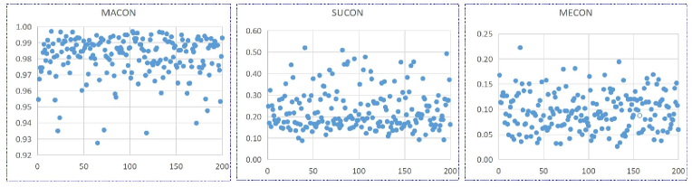
Fig. 6: For different methods to select sample confidence results, MACON can refer to Eq. 7, SUCON can refer to Eq. 8, and MECON can refer to Eq. 9.

Validation of Agent Collaboration Mode To verify the agent collaboration mode, we considered four modes. The first is to use two agents of the same structure (AgentMain+ AgentMain) and use the same datasets for training (MMOD); the second is to use two agents of the same structure (AgentMain+ AgentMain) and use two different datasets for training (MMTD); the third is to use two agents of different structures (AgentMain+ AgentCo) and use the same datasets for training (MCOD); the fourth is to use two agents of different structures (AgentMain+ AgentCo) and use two different datasets for training (MCTD). We directly use the selected samples to fine-tune the network, and the results are shown in Table 6. It can be seen from the results in Table 6 that the synergy effect of using two different structure models is better than that of using the same structure model. Using the same dataset to train the model to select key examples seems more important for agent update.

Table 6: F1 scores (%) for page segmentation on the DSSE-200. SN: The Number of sample.

Method	A	P	R	F1	SN
MMOD	68.6	66.4	69.8	68.1	19
MMTD	77.6	73.9	71.0	72.4	59
MCOD	78.1	79.2	77.9	78.5	23
MCTD	75.2	76.2	71.7	73.9	37

Validation of Key Samples Selection The previous classic methods used confidence as a measure of sample selection to deal with simple classification comparisons. DLA is a pixel-level classification task. We follow the work of Wan et al. [12] and replace the classification confidence with the new confidence. We choose the Three different confidence (Eq. 7, Eq. 8, Eq. 9) of the entire picture as the new confidence. The experimental results show as Fig. 6 that the confidence interval is (0.92, 1], (0, 0.6), and (0, 0.25)). As we can see in Fig. 5, there are local texts on the table or in the figure, so the confidence method is not applicable. We conducted experiments on DSSE-200 to compare the advantages of the sample selection strategy. We split DSSE-200 into the training set and test set according to 6:4. First, we use the model that trains by synthesis data to test directly on the test set (Baseline). Then, we randomly select x samples from the training set and use them fine-tuning models (Baseline+RDx), and finally, we use KSS to select the key samples (Find 18 key samples) and use them fine-tuning models. And the results are shown in Table 7. Obviously, compared with other methods, the KSS not only achieves better results but also uses very few training samples.

Table 7: F1 scores (%) for page segmentation on DSSE-200 dataset by ablation study.

Method	A	P	R	F1
Baseline	79.9	79.3	75.2	77.2
Baseline+RD20	81.3	80.2	81.5	80.8
Baseline+RD40	82.9	81.6	83.2	82.4
Baseline+RD60	84.5	84.7	86.9	85.8
KSS	85.6	86.2	86.3	86.2

Validation of Agent Update In order to compare the effects of our model update mode, we compared four model update methods. First, we use a simple fine-tuning mode, and our learning rate is generally reduced to 1/10 of the initial training (PSFT). We then use basic data and selected data for new fine-tuning and use the previous pre-trained model (PBSFT). Next, we use a model initialized only with random numbers for training and used basic data and selected data(RBSFT). The last one is the update method used by our framework (RBSRE).

It can be seen from the table  8 that only using key samples for fine-tuning results is not good. Because the number of key samples is limited, only using key samples for fine-tuning will push the model to overfit. Using a pre-training model can improve the performance of the model because the pre-training model contains more basic knowledge and can better improve the generalization of the model. The RBSRE can obtain better results, RBSRE not only considered key samples but also focus on the base samples.

Table 8: F1 scores (%) for page segmentation of Agent Update on the DSSE-200.

Method	A	P	R	F1
PSFT (Eq. 12)	68.9	70.1	68.2	69.1
PBSFT (Eq. 13)	82.7	81.6	82.5	82.0
RBSFT (Eq. 14)	78.6	77.5	79.3	78.4
RBSRE (Eq. 15)	86.2	85.1	87.5	86.3

5 Conclusions

In this paper, we proposed a key sample selection framework based on HITL named KSS. KSS includes three components: agent initialization, agent collaboration, and agent update. The agent initialization uses LaTex as a general sample generation engine to let the agent learn more common knowledge. We have innovatively proposed the multi-agent collaboration that realizes the selection of key samples. Hence, we revisited the learning system from reinforcement learning and designed a sample-based agent update strategy, which effectively improves the agent’s ability to accept new samples. To the best of our knowledge, this is the first work to introduce agent collaboration into HITL. Our results indicate that we have improved the state of the art on previously established benchmarks, and KSS can better find key samples by using fewer data.

Acknowledgment. This work was supported in part by the 2020 East China Normal University Outstanding Doctoral Students Academic Innovation Ability Improvement Project (YBNLTS2020-042), the Science and Technology Commission of Shanghai Municipality (19511120200).

References

- [1] G. M. Binmakhashen and S. A. Mahmoud, “Document layout analysis: a comprehensive survey,” ACM Computing Surveys (CSUR), vol. 52, no. 6, pp. 1–36, 2019.
- [2] D. He, S. Cohen, B. Price, D. Kifer, and C. L. Giles, “Multi-scale multi-task fcn for semantic page segmentation and table detection,” in International Conference on Document Analysis and Recognition (ICDAR), vol. 1, 2017, pp. 254–261.
- [3] C. Wick and F. Puppe, “Fully convolutional neural networks for page segmentation of historical document images,” in IAPR International Workshop on Document Analysis Systems (DAS), 2018, pp. 287–292.
- [4] Y. Li, Y. Zou, and J. Ma, “Deeplayout: A semantic segmentation approach to page layout analysis,” in International Conference on Intelligent Computing (ICIC), 2018, pp. 266–277.
- [5] Y. Li, P. Zhang, X. Xu, Y. Lai, F. Shen, L. Chen, and P. Gao, “Few-shot prototype alignment regularization network for document image layout segementation,” Pattern Recognition, vol. 115, p. 107882, 2021.
- [6] T. Lu and A. Dooms, “Probabilistic homogeneity for document image segmentation,” Pattern Recognition, vol. 109, p. 107591, 2021.
- [7] B. Zhou, A. Lapedriza, J. Xiao, A. Torralba, and A. Oliva, “Learning deep features for scene recognition using places database,” in Advances in Neural Information Processing Systems (NIPS), 2014, pp. 487–495.
- [8] F. Yu, A. Seff, Y. Zhang, S. Song, T. Funkhouser, and J. Xiao, “Lsun: Construction of a large-scale image dataset using deep learning with humans in the loop,” arXiv preprint arXiv:1506.03365, 2015.
- [9] J. Li, J. Yang, A. Hertzmann, J. Zhang, and T. Xu, “LayoutGAN: Synthesizing graphic layouts with vector-wireframe adversarial networks,” IEEE Transaction on Pattern Analysis and Machine Intelligence, 2020.
- [10] X. Liu, G. Yin, J. Shao, X. Wang et al., “Learning to predict layout-to-image conditional convolutions for semantic image synthesis,” in Advances in Neural Information Processing Systems (NIPS), 2019, pp. 570–580.
- [11] S. Zhao, Z. Liu, J. Lin, J.-Y. Zhu, and S. Han, “Differentiable augmentation for data-efficient gan training,” Advances in Neural Information Processing Systems (NIPS), vol. 33, 2020.
- [12] S. Wan, Y. Hou, F. Bao, Z. Ren, Y. Dong, Q. Dai, and Y. Deng, “Human-in-the-loop low-shot learning,” IEEE Transactions on Neural Networks and Learning Systems, 2020.
- [13] Z. Yue, H. Zhang, Q. Sun, and X.-S. Hua, “Interventional few-shot learning,” Advances in Neural Information Processing Systems (NIPS), vol. 33, 2020.
- [14] S. Zhang, L. He, E. Dragut, and S. Vucetic, “How to invest my time: Lessons from human-in-the-loop entity extraction,” in Annual ACM SIGKDD Conference on Knowledge Discovery and Data Mining (KDD), 2019, pp. 2305–2313.
- [15] X. Yang, E. Yumer, P. Asente, M. Kraley, D. Kifer, and C. Lee Giles, “Learning to extract semantic structure from documents using multimodal fully convolutional neural networks,” in Conference on Computer Vision and Pattern Recognition (CVPR), 2017, pp. 5315–5324.
- [16] C. A. Clark and S. Divvala, “Looking beyond text: Extracting figures, tables and captions from computer science papers,” in The AAAI Conference on Artificial Intelligence Workshops, 2015.
- [17] T. A. Tran, I.-S. Na, and S.-H. Kim, “Hybrid page segmentation using multilevel homogeneity structure,” in Proceedings of the International Conference on Ubiquitous Information Management and Communication (IMCOM), 2015, pp. 1–6.
- [18] M. Mehri, P. Héroux, P. Gomez-Krämer, and R. Mullot, “Texture feature benchmarking and evaluation for historical document image analysis,” International Journal on Document Analysis and Recognition (IJDAR), vol. 20, no. 1, pp. 1–35, 2017.
- [19] Y. Lu and C. L. Tan, “Constructing area voronoi diagram in document images,” in International Conference on Document Analysis and Recognition (ICDAR), 2005, pp. 342–346.
- [20] N. Vasilopoulos and E. Kavallieratou, “Complex layout analysis based on contour classification and morphological operations,” Engineering Applications of Artificial Intelligence, vol. 65, pp. 220–229, 2017.
- [21] A. Asi, R. Cohen, K. Kedem, and J. El-Sana, “Simplifying the reading of historical manuscripts,” in International Conference on Document Analysis and Recognition (ICDAR), 2015, pp. 826–830.
- [22] W. Swaileh, K. A. Mohand, and T. Paquet, “Multi-script iterative steerable directional filtering for handwritten text line extraction,” in International Conference on Document Analysis and Recognition (ICDAR), 2015, pp. 1241–1245.
- [23] F. Shafait and T. M. Breuel, “The effect of border noise on the performance of projection-based page segmentation methods,” IEEE Transaction on Pattern Analysis and Machine Intelligence, vol. 33, no. 4, pp. 846–851, 2010.
- [24] F. Shafait, J. Van Beusekom, D. Keysers, and T. M. Breuel, “Background variability modeling for statistical layout analysis,” in Proceedings of the International Conference on Pattern Recognition (ICPR), 2008, pp. 1–4.
- [25] K. Chen, F. Yin, and C.-L. Liu, “Hybrid page segmentation with efficient whitespace rectangles extraction and grouping,” in International Conference on Document Analysis and Recognition (ICDAR), 2013, pp. 958–962.
- [26] T. A. Tran, K. Oh, I.-S. Na, G.-S. Lee, H.-J. Yang, and S.-H. Kim, “A robust system for document layout analysis using multilevel homogeneity structure,” Expert Systems With Applications, vol. 85, pp. 99–113, 2017.
- [27] T. A. Tran, I. S. Na, and S. H. Kim, “Page segmentation using minimum homogeneity algorithm and adaptive mathematical morphology,” International Journal on Document Analysis and Recognition (IJDAR), vol. 19, no. 3, pp. 191–209, 2016.
- [28] D. Ravì, M. Bober, G. M. Farinella, M. Guarnera, and S. Battiato, “Semantic segmentation of images exploiting dct based features and random forest,” Pattern Recognition, vol. 52, pp. 260–273, 2016.
- [29] Y. Wang, J. Liu, Y. Li, J. Fu, M. Xu, and H. Lu, “Hierarchically supervised deconvolutional network for semantic video segmentation,” Pattern Recognition, vol. 64, pp. 437–445, 2017.
- [30] X. Wu, Z. Hu, X. Du, J. Yang, and L. He, “Document layout analysis via dynamic residual feature fusion,” in IEEE International Conference on Multimedia & Expo (ICME), 2021.
- [31] Y. Xu, F. Yin, Z. Zhang, and C.-L. Liu, “Multi-task layout analysis for historical handwritten documents using fully convolutional networks.” in International Joint Conference on Artificial Intelligence (IJCAI), 2018, pp. 1057–1063.
- [32] Y. Soullard, P. Tranouez, C. Chatelain, S. Nicolas, and T. Paquet, “Multi-scale gated fully convolutional densenets for semantic labeling of historical newspaper images,” Pattern Recognition Letters, vol. 131, pp. 435–441, 2020.
- [33] X. Zheng, X. Qiao, Y. Cao, and R. W. Lau, “Content-aware generative modeling of graphic design layouts,” ACM Transactions on Graphics (TOG), vol. 38, no. 4, pp. 1–15, 2019.
- [34] K. Li, C. Wigington, C. Tensmeyer, H. Zhao, N. Barmpalios, V. I. Morariu, V. Manjunatha, T. Sun, and Y. Fu, “Cross-domain document object detection: Benchmark suite and method,” in Conference on Computer Vision and Pattern Recognition (CVPR), 2020, pp. 12 915–12 924.
- [35] Y. Xu, M. Li, L. Cui, S. Huang, F. Wei, and M. Zhou, “Layoutlm: Pre-training of text and layout for document image understanding,” in ACM SIGKDD International Conference on Knowledge Discovery & Data Mining, 2020, pp. 1192–1200.
- [36] J. Long, E. Shelhamer, and T. Darrell, “Fully convolutional networks for semantic segmentation,” in Conference on Computer Vision and Pattern Recognition (CVPR), 2015, pp. 3431–3440.
- [37] D. D. Lewis and W. A. Gale, “A sequential algorithm for training text classifiers,” in Annual ACM Conference on Research and Development in Information Retrieval, 1994, pp. 3–12.
- [38] F. Ricci, L. Rokach, and B. Shapira, “Recommender systems: introduction and challenges,” in Recommender systems handbook, 2015, pp. 1–34.
- [39] C. Chai and G. Li, “Human-in-the-loop techniques in machine learning,” Data Engineering, p. 37, 2020.
- [40] T. Mandel, Y.-E. Liu, E. Brunskill, and Z. Popović, “Where to add actions in human-in-the-loop reinforcement learning,” in The AAAI Conference on Artificial Intelligence, vol. 31, no. 1, 2017.
- [41] H. S. Seung, M. Opper, and H. Sompolinsky, “Query by committee,” in Proceedings of the fifth annual workshop on Computational learning theory, 1992, pp. 287–294.
- [42] D. H. Grollman and O. C. Jenkins, “Dogged learning for robots,” in Proceedings of International Conference on Robotics and Automation, 2007, pp. 2483–2488.
- [43] S. Chernova and M. Veloso, “Interactive policy learning through confidence-based autonomy,” Journal of Artificial Intelligence Research, vol. 34, pp. 1–25, 2009.
- [44] K. Judah, A. Fern, and T. Dietterich, “Active imitation learning via state queries,” in Proceedings of International Conference on Machine Learning Workshops, 2011.
- [45] D. Silver, J. A. Bagnell, and A. Stentz, “Active learning from demonstration for robust autonomous navigation,” in Proceedings of International Conference on Robotics and Automation, 2012, pp. 200–207.
- [46] K. Judah, A. P. Fern, T. G. Dietterich, and P. Tadepalli, “Active imitation learning: Formal and practical reductions to iid learning,” Journal of Machine Learning Research, vol. 15, no. 120, pp. 4105–4143, 2014.
- [47] M. Ren, E. Triantafillou, S. Ravi, J. Snell, K. Swersky, J. B. Tenenbaum, H. Larochelle, and R. S. Zemel, “Meta-learning for semi-supervised few-shot classification,” in International Conference on Learning Representations (ICLR), 2018.
- [48] M. Andrychowicz, M. Denil, S. Gomez, M. W. Hoffman, D. Pfau, T. Schaul, B. Shillingford, and N. De Freitas, “Learning to learn by gradient descent by gradient descent,” in Advances in Neural Information Processing Systems (NIPS), 2016, pp. 3981–3989.
- [49] S. Gidaris and N. Komodakis, “Dynamic few-shot visual learning without forgetting,” in Conference on Computer Vision and Pattern Recognition (CVPR), 2018, pp. 4367–4375.
- [50] H. Yao, C. Zhang, Y. Wei, M. Jiang, S. Wang, J. Huang, N. Chawla, and Z. Li, “Graph few-shot learning via knowledge transfer,” in The AAAI Conference on Artificial Intelligence, vol. 34, no. 04, 2020, pp. 6656–6663.
- [51] G. Koch, R. Zemel, and R. Salakhutdinov, “Siamese neural networks for one-shot image recognition,” in Proceedings of International Conference on Machine Learning, vol. 2, 2015.
- [52] O. Vinyals, C. Blundell, T. Lillicrap, D. Wierstra et al., “Matching networks for one shot learning,” in Advances in Neural Information Processing Systems (NIPS), 2016, pp. 3630–3638.
- [53] J. Snell, K. Swersky, and R. Zemel, “Prototypical networks for few-shot learning,” in Advances in Neural Information Processing Systems (NIPS), 2017, pp. 4077–4087.
- [54] I. Goodfellow, J. Pouget-Abadie, M. Mirza, B. Xu, D. Warde-Farley, S. Ozair, A. Courville, and Y. Bengio, “Generative adversarial nets,” in Advances in Neural Information Processing Systems (NIPS), 2014, pp. 2672–2680.
- [55] X. Wu, K. Xu, and P. Hall, “A survey of image synthesis and editing with generative adversarial networks,” Tsinghua Science and Technology, vol. 22, no. 6, pp. 660–674, 2017.
- [56] G. Li, “Human-in-the-loop data integration,” Proceedings of the VLDB Endowment, vol. 10, no. 12, pp. 2006–2017, 2017.
- [57] M. Chevalier-Boisvert, D. Bahdanau, S. Lahlou, L. Willems, C. Saharia, T. H. Nguyen, and Y. Bengio, “Babyai: A platform to study the sample efficiency of grounded language learning,” in International Conference on Learning Representations (ICLR), 2018.
- [58] J.-C. Klie, R. E. de Castilho, and I. Gurevych, “From zero to hero: Human-in-the-loop entity linking in low resource domains,” in Proceedings of the Annual Meeting of the Association for Computational Linguistics, 2020, pp. 6982–6993.
- [59] T.-Y. Lin, M. Maire, S. Belongie, J. Hays, P. Perona, D. Ramanan, P. Dollár, and C. L. Zitnick, “Microsoft coco: Common objects in context,” in European Conference on Computer Vision (ECCV), 2014, pp. 740–755.
- [60] K. He, X. Zhang, S. Ren, and J. Sun, “Deep residual learning for image recognition,” in Conference on Computer Vision and Pattern Recognition (CVPR), 2016, pp. 770–778.
- [61] L.-C. Chen, G. Papandreou, I. Kokkinos, K. Murphy, and A. L. Yuille, “Deeplab: Semantic image segmentation with deep convolutional nets, atrous convolution, and fully connected crfs,” IEEE Transaction on Pattern Analysis and Machine Intelligence, vol. 40, no. 4, pp. 834–848, 2017.
- [62] F. Chollet, “Xception: Deep learning with depthwise separable convolutions,” in Conference on Computer Vision and Pattern Recognition (CVPR), 2017, pp. 1251–1258.
- [63] K. Simonyan and A. Zisserman, “Very deep convolutional networks for large-scale image recognition,” in International Conference on Learning Representations (ICLR), 2015.
- [64] M. Li, Y. Xu, L. Cui, S. Huang, F. Wei, Z. Li, and M. Zhou, “Docbank: A benchmark dataset for document layout analysis,” COLING, 2020.
- [65] M. Sarkar, M. Aggarwal, A. Jain, H. Gupta, and B. Krishnamurthy, “Document structure extraction using prior based high resolution hierarchical semantic segmentation,” in European Conference on Computer Vision (ECCV), 2020, pp. 649–666.
- [66] R. Sarkhel and A. Nandi, “Improving information extraction from visually rich documents using visual span representations,” Proceedings of the VLDB Endowment, vol. 14, no. 5, pp. 822–834, 2021.
- [67] C. Clark and S. Divvala, “Pdffigures 2.0: Mining figures from research papers,” in ACM/IEEE on Joint Conference on Digital Libraries (JCDL), 2016, pp. 143–152.
- [68] D. S. Bloomberg and L. Vincent, “Document image applications,” Morphologie Mathmatique, vol. 8, 2007.
- [69] S. S. Bukhari, F. Shafait, and T. M. Breuel, “Improved document image segmentation algorithm using multiresolution morphology,” in Document recognition and retrieval XVIII, vol. 7874, 2011, p. 78740D.
- [70] F. C. Fernández and O. R. Terrades, “Document segmentation using relative location features,” in Proceedings of the International Conference on Pattern Recognition (ICPR), 2012, pp. 1562–1565.
- [71] P. A. Praczyk and J. Nogueras-Iso, “Automatic extraction of figures from scientific publications in high-energy physics,” Information Technology and Libraries, vol. 32, no. 4, pp. 25–52, 2013.
- [72] V. Badrinarayanan, A. Kendall, and R. Cipolla, “Segnet: A deep convolutional encoder-decoder architecture for image segmentation,” IEEE Transaction on Pattern Analysis and Machine Intelligence, vol. 39, no. 12, pp. 2481–2495, 2017.
- [73] H. Zhao, J. Shi, X. Qi, X. Wang, and J. Jia, “Pyramid scene parsing network,” in Conference on Computer Vision and Pattern Recognition (CVPR), 2017, pp. 2881–2890.
- [74] H. Li, P. Xiong, J. An, and L. Wang, “Pyramid attention network for semantic segmentation,” in BMVC, 2018, p. 285.