Free Lunch for Co-Saliency Detection: Context Adjustment

Abstract

We unveil a long-standing problem in the prevailing co-saliency detection systems: there is indeed inconsistency between training and testing. Constructing a high-quality co-saliency detection dataset involves time-consuming and labor-intensive pixel-level labeling, which has forced most recent works to rely instead on semantic segmentation or saliency detection datasets for training. However, the lack of proper co-saliency and the absence of multiple foreground objects in these datasets can lead to spurious variations and inherent biases learned by models. To tackle this, we introduce the idea of counterfactual training through context adjustment and propose a “cost-free” group-cut-paste (GCP) procedure to leverage off-the-shelf images and synthesize new samples. Following GCP, we collect a novel dataset called Context Adjustment Training (CAT). CAT consists of 33,500 images, which is four times larger than the current co-saliency detection datasets. All samples are automatically annotated with high-quality mask annotations, object categories, and edge maps. Extensive experiments on recent benchmarks are conducted, show that CAT can improve various state-of-the-art models by a large margin (5$\%$ $\sim$ 25$\%$). We hope that the scale, diversity, and quality of our dataset can benefit researchers in this area and beyond. Our dataset will be publicly accessible through our project page.

Introduction

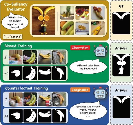
Figure 1: Conceptual illustration of counterfactual training versus biased training. Top block: Evaluations for the banana group in CoSOD3k (Fan et al. 2020); Middle block: Biased training samples from current co-saliency detection datasets; Bottom block: Samples generated under the idea of counterfactual training. GT denotes the ground-truth. Answers are generated by GICD (Zhang et al. 2020d).

Saliency detection attempts to mimic the human visual system by automatically detecting and segmenting out object regions that attract the most attention in an image (Borji et al. 2019). Today’s saliency detection systems, especially those equipped with deep neural networks (Wang et al. 2021) are good at identifying salient objects from images (Borji et al. 2019). However, the setting of detecting a single object is less practical. For real-world applications like image/video retrieval (Jerripothula, Cai, and Yuan 2019), surveillance (Gao et al. 2020), video analysis (Jerripothula, Cai, and Yuan 2016), etc., there are always scenes with multiple objects co-occurring in or across frames. This motivates our community to explore co-saliency detection (Jacobs, Goldman, and Shechtman 2010). Sharing a similar rationale with saliency detection, co-saliency detection automatically detects and segments out the common object regions that attract the most attention within image groups (Wang et al. 2021). Such an imitation can be achieved by the learning paradigm hiding behind artificial neural networks, especially convolutional neural networks (LeCun et al. 1998). However, “there is no such thing as a free lunch”. The success of deep learning systems depends heavily on large-scale datasets, which take huge effort and time to collect. The conventional way (Fan et al. 2020; Zhang et al. 2020d) of constructing a specialized co-saliency detection dataset involves time-consuming and labor-intensive data selection and pixel-level labeling. As shown in Figure 1, the uni-object distribution of the current training data (middle block) has deviated heavily from that of the evaluation data (top block), which consists of complex context with multiple foreground objects. Models encoded with such spurious variations and biases fail to capture the co-salient signals and thus make incorrect predictions (Torralba and Efros 2011; Herranz, Jiang, and Li 2016).

In the context of co-saliency detection, we denote the training, testing, and true (real-world) distributions as $\mathcal{D}$, $\mathcal{E}$, and $\mathcal{T}$, respectively. Recent works on evaluation (Fan et al. 2020; Zhang et al. 2020d) make $\mathcal{E}$ one-step closer towards $\mathcal{T}$ by identifying co-salient signals from multi-foreground clusters in a group-by-group manner. However, a dataset that can well-define $\mathcal{D}$ is still missing. As we will discuss in the next section, most recent works borrow semantic segmentation datasets like MS-COCO (Lin et al. 2014) and saliency detection datasets like DUTS (Wang et al. 2017) to train their models, which exacerbate the inconsistency among $\mathcal{D}$, $\mathcal{E}$, and $\mathcal{T}$. Not surprisingly, as models only see naive examples during training, they will inevitably cater to the seen idiosyncrasies, and thus are stuck in the unseen world with biased assumptions. In this paper, we aim at finding a “cost-free” way to handle the distribution inconsistency in co-saliency detection. Intrigued by causal effect (Pearl and Mackenzie 2018; Pearl, Glymour, and Jewell 2016) and its extensions in vision & language (Wang et al. 2020; Niu et al. 2021; Yue et al. 2020), we introduce counterfactual training with regard to the gap between current training distribution $\mathcal{D}$ and true distribution $\mathcal{T}$ as the direct cause (Pearl 2013; Tang, Huang, and Zhang 2020) of incorrect co-saliency predictions. As shown in Figure 2, the quality of prediction $\mathcal{P}$ made by a learning-based model is dependent on the quality of input data $\mathcal{I}$ under distribution $\mathcal{D}$. The goal of counterfactual training is to synthesize “imaginary” data sample $\hat{\mathcal{I}}$, whose distribution $\hat{\mathcal{D}}$ — also originates from $\mathcal{D}$ — can mimic $\mathcal{T}$. In this way, models can capture the true effect in terms of co-saliency from $\hat{\mathcal{I}}$ and make prediction $\hat{\mathcal{P}}$ properly.

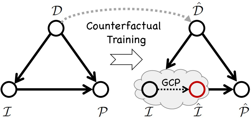
Figure 2: Causal graph for co-saliency detection. Circle nodes denote variables and arrows denote direct causal effects.

Under the instruction of counterfactual training, we propose using context adjustment (Divvala et al. 2009) to augment off-the-shelf saliency detection datasets, and introduce a novel group-cut-paste (GCP) procedure to improve the distribution of the training dataset. Taking a closer look at Figure 1. $\mathcal{M}$ and $\mathcal{Y}$ are the corresponding pixel-level annotation and category label of sample $\mathcal{I}$. GCP turns $\mathcal{I}$ into a canvas to be completed and paint the remaining part through the following steps: (1) classifying candidate images into a semantic group $\mathcal{Z}$ (e.g., banana) by reliable pretrained models; (2) cutting out candidate objects (e.g., baseball, butterfly, etc.); and (3) pasting candidate objects into image samples. We will revisit this procedure formally in the following sections. Different from the plain “observation” (e.g., different color from the background) made by biased training, counterfactual training opens the door of “imagination” and allows models to think comprehensively (Niu et al. 2021). A better prediction can be made possibly because of features, such as the elongated and curved shape (instead of the round shape of baseball and orange) or yellow-green color (instead of the dark color of remote control and avocado), are captured. In this way, models can focus more on the true causal effects rather than spurious variations and biases caused by the distribution gap (Chen et al. 2020).

Following GCP, we collect a novel dataset called Context Adjustment Training (CAT). Our dataset consists of $280$ subclasses affiliated to $15$ superclasses, which cover common items in daily life, as well as animals and plants in nature. While CAT is diverse in semantics, it also has a large scale. A total number of 33,500 training samples making it the current largest in co-saliency detection. Every sample in CAT is equipped with sophisticated mask annotation, category, and edge information. It is worth noting that, unlike expensive data selection and pixel-by-pixel labeling, all the images and their corresponding masks in our dataset are automatically synthesized and annotated, making the cost virtually “free”. Extensive experiments verify the effectiveness of our dataset. Without bells and whistles, CAT helps both one-stage and two-stage models to achieve significant improvements for on average 5$\%$ $\sim$ 25$\%$ in conventionally-adopted metrics on the challenging evaluation datasets CoSOD3k (Fan et al. 2020) and CoCA (Zhang et al. 2020d).

Related Work

#	Dataset	Year	#Img.	#Cat.	#Avg.	#Max.	#Min.	Mul.	Sal.	Larg.	H.Q.	Type	Inputs
1	MSRC	2005	240	8	30.0	30	30	✗	✓	✗	✗	CO	Group images
2	iCoseg	2010	643	38	16.9	41	4	✗	✓	✗	✓	CO	Group images
3	CoSal2015	2015	2,015	50	40.3	52	26	✓	✓	✗	✓	CO	Group images
4	DUTS-TR	2017	10,553	-	-	-	-	✗	✓	✓	✓	SD	Single image
5	COCO9213	2017	9,213	65	141.7	468	18	✓	✓	✗	✗	SS	Group images
6	COCO-GWD	2019	9,000	118	76.2	-	-	✓	✓	✗	✗	SS	Group images
7	COCO-SEG	2019	200,932	78	2576.1	49,355	201	✓	✗	✓	✗	SS	Group images
8	WISD	2019	2,019	-	-	-	-	✓	-	✗	-	CO	Single image
9	DUTS-Class	2020	8,250	291	28.3	252	5	✗	✓	✓	✓	CO	Group images
10	CAT (Ours)	2021	33,500	280	119.6	824	28	✓	✓	✓	✓	CO	Group images

Table 1: Datasets used for training co-saliency detection models. #Img.: Number of images; #Cat.: Number of categories; #Avg.: Average number of images per category; #Max.: Maximum number of images per group; #Min.: Minimum number of images per group. Mul.: Whether contains multiple foreground objects or not; Sal.: Whether maintains saliency or not; Larg.: Whether large-scale (more than 10k images) or not; H.Q.: Whether has high-quality annotations or not. CO: Co-saliency detection dataset; SD: Saliency detection dataset; SS: Semantic segmentation dataset. “-” denotes “not available”.

Context Adjustment. Modeling visual contexts liberates a lot of computer vision tasks from the impediment caused by the need for sophisticated annotations (Dwibedi, Misra, and Hebert 2017), such as bounding boxes and pixel-level masks. (Yun et al. 2019a) leverages training pixels and regularization effects of regional dropout by cutting and pasting image patches. To avoid overfitting, (DeVries and Taylor 2017) randomly masks out square regions of an image during training. The generic vicinal distribution introduced in (Zhang et al. 2018) helps to synthesize the groundtruth of new samples by the linear interpolation of one-hot labels. Unfortunately, the patches introduced by both (Yun et al. 2019a) and (DeVries and Taylor 2017) may cause severe occlusions for the original objects, which is not compatible with the idea of saliency detection (Fan et al. 2018a). For (Zhang et al. 2018), the local statistics and semantic are destroyed. Since the foreground and background are blended, the saliency cannot be appropriately defined anymore. (Hendrycks et al. 2020) fixes this problem by mixing several transformed versions of an image together, i.e., augmentation chain. Although such a composition improves the model robustness, it cannot introduce co-salient signals. (Zhang et al. 2020d) concatenates two samples together to form a multi-foreground image. However, for backbones that require fixed-size inputs (Simonyan and Zisserman 2015), the resize of such jigsawed images leads to severe shape distortion. In contrast, our GCP preserves both the multi-foreground requirement and object shapes and maintains saliency (Fan et al. 2018a).

Co-Saliency Detection. The origin of this task can be dated back to the last decade (Jacobs, Goldman, and Shechtman 2010), where co-saliency was defined as the regions of an object which occurs in a pair of images (Li and Ngan 2011). A more formal definition given in (Li, Meng, and Ngan 2013) exploits both intra- and inter-image saliency in a group-by-group manner. Since then, researchers in this area have been working on identifying co-salient signals across image groups (Cheng et al. 2014a). Representative works from early years (Chen 2010; Fu, Cao, and Tu 2013; Liu et al. 2014) rely on certain heuristics like background priors (Yao et al. 2017) and color contrasts (Cong et al. 2017). Let alone the post-processing like CRF (Krähenbühl and Koltun 2011), most modern co-saliency detection models can be divided into two-stage and one-stage models. Building upon saliency detection frameworks, two-stage models leverage the intra-saliency with inter-saliency generated by specially designed modules (Jin et al. 2020; Fan et al. 2021a). There are also some one-stage models which do not require saliency preparation. (Zhang et al. 2020c), (Zhang et al. 2020d), and (Fan et al. 2021b) introduce consensus embedding procedures to explore group representation and use it to guide soft attentions (Zhou et al. 2016). Associating with our dataset, both the state-of-the-art two-stage and one-stage models achieve better performances.

Datasets. Due to the lack of a suitable training dataset, most previous works use existing saliency detection datasets or semantic segmentation datasets for training. Table 1 summarizes datasets adopted to train co-saliency detection models. Small datasets (Winn, Criminisi, and Minka 2005; Batra et al. 2010; Dai et al. 2013) are popular among works in early years only. Some large-scale saliency detection datasets (Yang et al. 2013; Cheng et al. 2014b; Wang et al. 2017) are adopted by two-stage models to extract intra-saliency cues. However, such datasets do not have class information and multiple foreground objects, hence it is impossible for them to train end-to-end co-saliency detection models. Some works even borrow datasets from semantic segmentation, e.g., COCO-SEG (Wang et al. 2019) and COCO9213 (Lin et al. 2014). Unfortunately, although such datasets are large in scales, their annotations are coarse. Recently, DUTS-Class (Zhang et al. 2020d) and its jigsawed version (Zhang et al. 2020d) have been proposed as a “transition plan” towards co-saliency. However, the former is just a “grouped” saliency detection dataset, while the latter introduces issues like shape distortion and independent boundaries. Evidence shows that these inappropriate training paradigms have caused serious biases for co-saliency detection models (Fan et al. 2020; Zhang et al. 2020d). Our dataset addresses the aforementioned problems. CAT is currently the largest co-saliency detection dataset and offers diverse semantics and high-quality annotations.

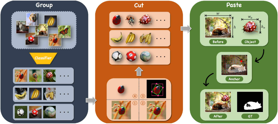
Figure 3: Overview of our group-cut-paste (GCP) procedure. Left block: Classifier $\mathcal{F(\cdot)}$ generates category label $\mathcal{Y}$ for all raw images and “group” them accordingly; Middle block: Object $o$ is “cut” out from the original image based on contours $\{(p,q)_{n}\}$ and bounding boxes; Right block: New sample $\hat{\mathcal{I}}$ is synthesized by “pasting” randomly sampled object $o$ into canvas $\mathcal{I}$.

Proposed Method

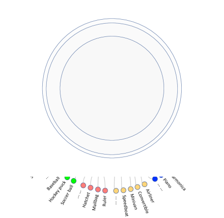
Figure 4: The taxonomic illustration for our dataset, of which consists of 15 superclasses and 280 subclasses. Zoom in for details.

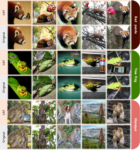
Figure 5: Samples from our dataset. Zoom in for details.

In this section, we first introduce the idea of counterfactual training in co-saliency detection. Under this high-level instruction, we propose a group-cut-paste (GCP) procedure to adjust visual context and generate training samples. Finally, we construct a novel dataset by following GCP.

Counterfactual Training

Let $\mathcal{I}\in\mathbb{R}^{w\times h\times c}$ and $\mathcal{M}\in\mathbb{R}^{w\times h}$ denote a training image and its mask annotation with width $w$, height $h$, and channel $c$. $\mathcal{Z}$ is an image group whose members include $\mathcal{I}$. $\mathcal{Y}$ denotes the category label which contains the semantic information for both $\mathcal{Z}$ and $\mathcal{I}$. The counterfactual (Pearl 2009) $\hat{\mathcal{I}}=\mathcal{I}_{\mathcal{M}}[\hat{\mathcal{Z}}(\hat{\mathcal{I}})]$ of sample $\mathcal{I}$, is read as:

         $\mathcal{I}$ would be $\hat{\mathcal{I}}$, had $\mathcal{M}$ been $\hat{\mathcal{M}}$,        given the fact that $\mathcal{Z}=\hat{\mathcal{Z}}(\mathcal{I}=\hat{\mathcal{I}})$.

where $\hat{\mathcal{Z}}\supset\hat{\mathcal{I}}$ denotes the new image group; New mask is restricted as $\hat{\mathcal{M}}\approx\mathcal{M}$ to maintain the saliency (Fan et al. 2018a) of the co-occurring object. In other words, label $\mathcal{Y}$ will not change during the whole process. The given “fact” $\mathcal{Z}=\hat{\mathcal{Z}}(\hat{\mathcal{I}})$ means that the group training paradigm remains the same, while the “counter-fact” (what if) $\mathcal{M}\neq\hat{\mathcal{M}}(\hat{\mathcal{I}})$ is indicating that the generated $\hat{\mathcal{M}}(\hat{\mathcal{I}})$ clashes with $\hat{\mathcal{M}}$.

The conceptual meanings of counterfactual training can be substantiated by the following instructions (Pearl, Glymour, and Jewell 2016):

Abduction - “Given the fact that $\mathcal{Z}=\hat{\mathcal{Z}}(\mathcal{I}=\hat{\mathcal{I}})$”. When constructing a new image group $\hat{\mathcal{Z}}$ for $\mathcal{Z}$, the co-saliency should remain unchanged. That is to say, the “fact” that the object in $\mathcal{I}\subset\mathcal{Z}$ is salient still holds for it in $\hat{\mathcal{I}}\subset\hat{\mathcal{Z}}$.

Action - “Had $\mathcal{M}$ been $\hat{\mathcal{M}}$”. After the “imagination”, the mask annotation $\hat{\mathcal{M}}$ should not have a significant change. Here we intervene $\mathcal{M}$ by keeping the semantic label $\mathcal{Y}$ the same both beforehand and afterhand.

Prediction - “$\mathcal{I}$ would be $\hat{\mathcal{I}}$”. Conditioning on the “fact” $\mathcal{Z}=\hat{\mathcal{Z}}(\hat{\mathcal{I}})$ and the intervention objective $\mathcal{M}\approx\hat{\mathcal{M}}$, we can generate the counterfactual sample $\hat{\mathcal{I}}$ and its mask $\hat{\mathcal{M}}$ from the following probability distribution function: $P(\mathcal{I}\mid\mathcal{Z}=\hat{\mathcal{Z}}(\hat{\mathcal{I}}),\mathcal{M}\approx\hat{\mathcal{M}})$.

Group-Cut-Paste

Following the counterfactual training instructions, we design the group-cut-paste (GCP) procedure. Specifically, the object map $\mathcal{O}\in\mathbb{R}^{w\times h\times c}$ for image $\mathcal{I}$ can be generated via $\mathcal{M}$, i.e., $\mathcal{O}=\mathcal{I}\odot\mathcal{M}$, where $\odot$ denote element-wise multiplication. The goal of GCP is to automatically generate new training sample $(\hat{\mathcal{I}},\hat{\mathcal{M}})$ by combing $\mathcal{I}_{a}$ and $\mathcal{M}_{a}$ with $\mathcal{O}_{b}$, where $a$ and $b$ are category indexes of the target and source groups, respectively. The generated sample $(\hat{\mathcal{I}},\hat{\mathcal{M}})$ is then used to train candidate models with their original loss functions. Figure 3 gives an overview of our method.

Group. The first step is to build image groups. To effectively classify candidate images, we adopt one of the current state-of-the-art classifiers WSL-Images (Mahajan et al. 2018), which achieves $85.4\%$ Top-1 accuracy on ImageNet (Deng et al. 2009). The category label $\mathcal{Y}$ can be generated via $\mathcal{Y}=\mathcal{F}(\mathcal{I})$, where $\mathcal{F(\cdot)}$ denotes the pretrained classifier. We manually pick out the misclassified examples after grouping. This results in $\{(\mathcal{I},\mathcal{Y}),\mathcal{M}\}$ sample pairs distributed in $z$ semantic groups.

Cut. Both object map $\mathcal{O}$ and mask $\mathcal{M}$ are used to prepare candidate object $o$. We adopt the border following algorithm (Suzuki 1985) to extract $n$ external contour points $\{(p,q)_{n}\}$ by mask $\mathcal{M}$. Based on contours, the bounding rectangle with minimum area can be drawn. The area to be cut can then be defined by the four vertices of this rotated box. This gives us the final object $o\in\mathbb{R}^{w_{o}\times h_{o}\times c}$.

Paste. Under the counterfactual training instructions, object $o$ can be pasted properly into $\mathcal{I}$ to form a new sample $\hat{\mathcal{I}}$. Here we maintain the “fact” by preserving group consistency, i.e., conduct this procedure in a group-by-group manner. Denote the regions outside $\mathcal{M}$ as $\bar{\mathcal{M}}$. To avoid severe occlusion, coordinate $(x,y)$ is randomly sampled in $\bar{\mathcal{M}}$ as the position to be pasted. The center of $o$ is chosen as the anchor for pasting. We execute the “action” by restricting the size of candidate object $o$ and maintaining label $\mathcal{Y}$ before and after paste. The mask annotations $\hat{\mathcal{M}}$ are automatically synthesized by dyadic operations between $o$ and $\mathcal{M}$. Finally, under uniform probability distribution $P=1/(z-1)$, “prediction” gives us $\{(\hat{\mathcal{I}},\mathcal{Y}),\hat{\mathcal{M}\}}$ pairs for further model training. Our GCP operation can be easily applied on CPUs in parallel with the main GPU training tasks, which hides the computation cost and boosts the performance for virtually free.

Constructing the Dataset

For the purpose of stabilization and to ensure high quality, we collect a dataset called Context Adjustment Training (CAT). We pick 8,375 images with clear saliency and sophisticated annotations as our canvas from existing saliency detection datasets (Wang et al. 2017; Fan et al. 2018a). Following GCP, 280 semantic groups affiliated to 15 superclasses are built after the “grouping”, i.e., aves, electronic product (elec.), food, fruit, insect, instrument (instru.), kitchenware (kitch.), mammal (mamm.), marine, other, reptile (rept.), sports, tool, transportation (trans.), and vegetable (vege.). See Figure 4 for the taxonomy. We then “cut” all the objects $o$ out and discard those with incomplete shapes. During the “paste” stage, the object size is restricted as $\frac{w_{o}}{w}=\frac{h_{o}}{h}=(0.1\sim 0.8)$. Candidate objects are randomly flipped horizontally to increase diversity. We sample twice for each candidate image to generate two samples and do a re-sample for unsatisfied cases. This gives us 16,750 augmented images. Their corresponding masks are automatically generated. As shown in Figure 5, samples synthesized by counterfactual training and GCP can model realistic visual context and offer proper co-salient signals. Following (Zhang et al. 2020d), we expand the scale of our dataset by supplementing twice as many samples without augmentation. In total, CAT consists of 33,500 images, which is ten times and four times bigger than the current largest co-saliency detection evaluation set and training set, respectively. See Table 1 for more dataset statistics. Several group patterns (calculated by averaging overlapping masks) of our dataset are shown in Figure 6. The overall pattern of our dataset tends to be a “round” shape, while categories with unique shapes (e.g., cello and limousine) result in shape-biased patterns, which is consistent with the definition of saliency (Fan et al. 2018a). More details of our dataset can be found in the supplementary material.

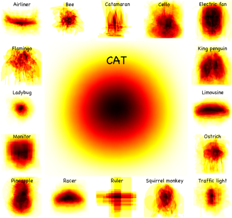
Figure 6: Patterns for representative groups and the overall dataset. Best viewed in color and zoomed-in for details.

Benchmark Experiment

In this section, we conduct a comprehensive benchmark study for co-saliency detection to verify the effectiveness and superiority of our proposed methods and dataset.

Implementation Details

Competitors. We compare our dataset with six representative datasets and four popular augmentation techniques, i.e., COCO-SEG (Wang et al. 2019), DUTS-TR (Wang et al. 2017), COCO9213 (Lin et al. 2014), CoSal2015 (Zhang et al. 2016), DUTS-Class (Zhang et al. 2020d), AutoAug (Cubuk et al. 2019), CutOut (DeVries and Taylor 2017), CutMix (Yun et al. 2019b), and Jigsaw (Zhang et al. 2020d).

Models. Five state-of-the-art models with open-sourced code are selected for our benchmark experiments, i.e., PoolNet (Liu et al. 2019), EGNet (Zhao et al. 2019), ICNet (Jin et al. 2020), GICD (Zhang et al. 2020d), and GCoNet (Fan et al. 2021b). All training configurations w.r.t. model architectures, hyperparameters, loss functions, and other tricks are kept default except for learning rate. For each dataset, we tune the learning rate a bit with multiple runs to ensure the convergence and report the average results to avoid extreme cases. NVIDIA GeForce RTX 2080Ti graphics cards are used through our experiments. Due to space limits, please refer to the supplementary for more configuration details.

Dataset	MAE $\downarrow$	$F_{max}$ $\uparrow$	$E_{avg}$ $\uparrow$	$S_{\alpha}$ $\uparrow$	MAE $\downarrow$	$F_{max}$ $\uparrow$	$E_{avg}$ $\uparrow$	$S_{\alpha}$ $\uparrow$
CoSal2015	0.181	0.510	0.629	0.578	0.199	0.315	0.577	0.508
DUTS-TR‡	0.209	0.518	0.646	0.620	0.235	0.299	0.558	0.525
DUTS-Class	0.205	0.508	0.649	0.591	0.210	0.323	0.594	0.535
COCO9213	0.225	0.488	0.639	0.601	0.256	0.283	0.541	0.509
mygrayCAT	mygray0.171	mygray0.561	mygray0.689	mygray0.636	mygray0.181	mygray0.346	mygray0.625	mygray0.561

Table 2: Benchmarking results of different datasets trained by PoolNet (Liu et al. 2019) and evaluated on CoSOD3k (left) and CoCA (right).

Dataset	MAE $\downarrow$	$F_{max}$ $\uparrow$	$E_{avg}$ $\uparrow$	$S_{\alpha}$ $\uparrow$	MAE $\downarrow$	$F_{max}$ $\uparrow$	$E_{avg}$ $\uparrow$	$S_{\alpha}$ $\uparrow$
CoSal2015	0.103	0.698	0.791	0.754	0.159	0.430	0.649	0.615
DUTS-TR‡	0.118	0.696	0.771	0.760	0.182	0.425	0.610	0.604
DUTS-Class	0.113	0.704	0.793	0.770	0.166	0.440	0.640	0.620
COCO9213	0.122	0.702	0.781	0.762	0.178	0.430	0.635	0.613
mygrayCAT	mygray0.088	mygray0.745	mygray0.830	mygray0.791	mygray0.143	mygray0.449	mygray0.678	mygray0.626

Table 3: Benchmarking results of different datasets trained by EGNet (Zhao et al. 2019) and evaluated on CoSOD3k (left) and CoCA (right).

Dataset	MAE $\downarrow$	$F_{max}$ $\uparrow$	$E_{avg}$ $\uparrow$	$S_{\alpha}$ $\uparrow$	MAE $\downarrow$	$F_{max}$ $\uparrow$	$E_{avg}$ $\uparrow$	$S_{\alpha}$ $\uparrow$
DUTS-Class	0.088	0.761	0.835	0.798	0.148	0.473	0.667	0.637
COCO9213‡	0.089	0.762	0.840	0.794	0.147	0.513	0.683	0.654
mygrayCAT	mygray0.068	mygray0.791	mygray0.866	mygray0.811	mygray0.108	mygray0.529	mygray0.734	mygray0.673
DUTS-Class	0.089	0.758	0.834	0.793	0.146	0.469	0.677	0.634
COCO9213‡	0.095	0.767	0.835	0.797	0.155	0.522	0.670	0.653
mygrayCAT	mygray0.067	mygray0.792	mygray0.867	mygray0.817	mygray0.101	mygray0.533	mygray0.743	mygray0.678

Table 4: Benchmarking results of different datasets trained by ICNet (Jin et al. 2020) and evaluated on CoSOD3k (left) and CoCA (right). Row 2-4: SISMs generated by EGNet with VGG backbone; Row 5-7: SISMs generated by EGNet with ResNet backbone.

Dataset	MAE $\downarrow$	$F_{max}$ $\uparrow$	$E_{avg}$ $\uparrow$	$S_{\alpha}$ $\uparrow$	MAE $\downarrow$	$F_{max}$ $\uparrow$	$E_{avg}$ $\uparrow$	$S_{\alpha}$ $\uparrow$
COCO-SEG	0.080	0.767	0.853	0.793	0.133	0.508	0.695	0.654
DUTS-Class‡	0.081	0.766	0.845	0.802	0.150	0.475	0.656	0.632
COCO9213	0.084	0.753	0.839	0.783	0.143	0.499	0.679	0.641
mygrayCAT	mygray0.070	mygray0.786	mygray0.863	mygray0.812	mygray0.116	mygray0.523	mygray0.716	mygray0.668

Table 5: Benchmarking results of different datasets trained by GICD (Zhang et al. 2020d) and evaluated on CoSOD3k (left) and CoCA (right).

Dataset	MAE $\downarrow$	$F_{max}$ $\uparrow$	$E_{avg}$ $\uparrow$	$S_{\alpha}$ $\uparrow$	MAE $\downarrow$	$F_{max}$ $\uparrow$	$E_{avg}$ $\uparrow$	$S_{\alpha}$ $\uparrow$
COCO-SEG	0.084	0.755	0.842	0.780	0.119	0.527	0.720	0.656
DUTS-Class	0.074	0.771	0.850	0.802	0.122	0.513	0.704	0.657
COCO9213	0.081	0.751	0.839	0.779	0.120	0.520	0.710	0.654
mygrayCAT	mygray0.065	mygray0.789	mygray0.862	mygray0.813	mygray0.089	mygray0.531	mygray0.728	mygray0.673

Table 6: Benchmarking results of different datasets trained by GCoNet (Fan et al. 2021b) and evaluated on CoSOD3k (left) and CoCA (right).

Method	MAE $\downarrow$	$F_{max}$ $\uparrow$	$F_{avg}$ $\uparrow$	$E_{max}$ $\uparrow$	$E_{avg}$ $\uparrow$	$S_{\alpha}$ $\uparrow$
RandomFlip	0.080	0.766	0.754	0.851	0.840	0.795
RandomRotate	0.103	0.729	0.718	0.831	0.819	0.767
AutoAug	0.098	0.732	0.723	0.836	0.821	0.779
CutOut	0.110	0.715	0.707	0.812	0.807	0.762
CutMix	0.087	0.745	0.739	0.839	0.836	0.772
Jigsaw	0.079	0.770	0.763	0.848	0.845	0.797
mygrayGCP	mygray0.073	mygray0.802	mygray0.785	mygray0.866	mygray0.849	mygray0.804

Table 7: Comparison among different augmentation techniques associated with GICD (Zhang et al. 2020d) and evaluated on CoSOD3k.

#	Group	Cut	Paste	MAE $\downarrow$	$F_{max}$ $\uparrow$	$F_{avg}$ $\uparrow$	$E_{max}$ $\uparrow$	$E_{avg}$ $\uparrow$	$S_{\alpha}$ $\uparrow$
A	$\diamond$			.203	.419	.413	.612	.601	.591
B	✓			.150	.472	.466	.679	.663	.633
C	$\diamond$		$\diamond$	.178	.408	.402	.631	.622	.582
D	$\diamond$	✓	$\diamond$	.173	.417	.411	.648	.635	.586
E	✓		$\diamond$	.139	.460	.456	.699	.691	.627
F	✓	✓	$\diamond$	.130	.474	.469	.700	.692	.638
Ours	✓	✓	✓	.102	.522	.510	.721	.711	.662

Table 8: Ablation study for our proposed GCP approach with GICD (Zhang et al. 2020d) on the CoCA dataset. Symbols ✓and $\diamond$ denote conduct and randomly conduct corresponding operations, respectively.

Evaluation. We adopt the two recent and popular evaluation datasets CoSOD3k (Fan et al. 2020) and CoCA (Zhang et al. 2020d) to evaluate model performances. Four conventional metrics are adopted: mean absolute error (MAE) (Cheng et al. 2013), F-measure (Achanta et al. 2009), E-measure (Fan et al. 2018b), and structure measure ($S_{\alpha}$) (Fan et al. 2017). For F-measure (Achanta et al. 2009), we follow the convention by setting weight ${\beta}^{2}=0.3$ and report both the maximum score ($F_{max}$) and the mean score ($F_{avg}$). We also report both $E_{max}$ and $E_{min}$ for E-measure (Fan et al. 2018b). We use symbols $\uparrow$ and $\downarrow$ to denote the metrics which are the higher and the lower the better, respectively. Superscript ^‡ denotes the reported results or results reproduced by public checkpoints.

Quantitative Analysis

Longitudinal Comparison. From Tables 2 - 6, we observe that all models trained on CAT achieve better results than other datasets in all metrics on both CoSOD3k and CoCA. This suggests that CAT is agnostic to models and backbones. Specifically, the improvements are typically larger in MAE. Significant boosts for on average more than $25\%$ are achieved on PoolNet, EGNet, ICNet, and GCoNet, as well as a gain around $18\%$ on GICD. Regarding the average improvements on other metrics, we observe that CAT improves more on $F$ ($\sim 9\%$), which shows that instead of radically regarding every foreground objects as salient, models trained on CAT tend to make relatively conservative predictions and focus more on regions with co-salient objects only. This supports our analysis in the previous sections. It also provides improvements in $E$ ($\sim 7\%$) and $S_{\alpha}$ ($\sim 5\%$). Indeed, $S_{\alpha}$ is the hardest among metrics which measures both accuracy and structural similarity. Although models are capable of making more confident predictions now, they cannot capture very detailed information like boundaries. Overall, we believe that the diversity and quality of CAT have laid a solid foundation for more in-depth works in the future.

Horizontal Comparison. Changing the direction of comparison, we notice that the evaluation scores on CoSOD3k are much higher than CoCA. This is in line with the characteristics of these two datasets: although the former is richer in scale, the latter has more complex context and more variant appearance, such as occlusion and object size. Besides, the performances of co-saliency detection models are much better than that of saliency detection models, which emphasize again the importance of specialized modules/techniques designed for identifying co-salient signals and suppressing non-salient ones. As for different augmentation techniques (see Table 7), they share a common problem during training: instability. For those without considerations of co-saliency like AutoAug, CutOut, and CutMix, the performances are degraded. Only Jigsaw and our GCP procedure surpass the baseline and the latter offers even larger improvements.

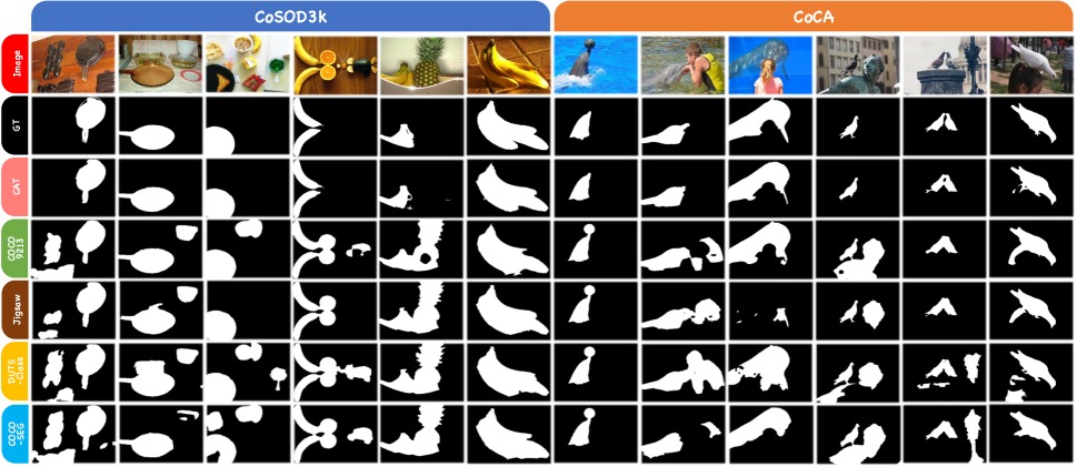
Figure 7: Qualitative results of different datasets trained by GICD (Zhang et al. 2020d). Left: results on CoSOD3k (Fan et al. 2020); Right: results on CoCA (Zhang et al. 2020d). Groups from left to right: frying pan, banana, dolphin, and pigeon.

Ablation Study. We conduct an ablation study to verify the effectiveness of our methods (see Table 8). The results for the original 8,375 images are shown in rows A and B. We also provide other combinations for comparisons, e.g., group images w/ classifiers (vs. randomly allocate images to the same number of groups), cut candidate objects out before paste (vs. do not cut and paste the sampled images directly), and paste objects/images under counterfactual rules (vs. no paste or randomly paste w/o limitations). Specifically, “Group” offers proper inter-saliency signals, which is essential for models to find the common salient objects between image groups (A vs. B, C vs. E). “Cut” gives fine-grained category information and further improves performance (C vs. D, E vs. F). As the key part, “Paste” provides intra-saliency signals, which determines the quality of the collaborative learning paradigm. A proper introduction of such signals significantly boosts the performance (Ours vs. F), and vice versa (A vs. C, B vs. E).

Qualitative Analysis

Figure 7 illustrates some visualizations among different competitors on CoSOD3k and CoCA generated by GICD. It can be easily observed that the quality of a dataset plays an important role for model training. Models encoded with features from high-quality dataset like CAT tends to focus more on the true co-salient signals while suppressing the non-salient ones. Taking the frying pan group as an example. Both semantic segmentation and saliency detection datasets fail to teach the model “what” and “where” to focus and thus let it mistakenly regards items besides frying pans as co-salient. In contrast, the model trained on CAT can well distinguish co-salient objects from non-salient clusters even when they share similar shapes, textures, colors, etc. We refer to the supplementary for more examples. Another point worthy of attention is that the existing models cannot well-restore the details (e.g., the boundaries) of objects, especially that of small objects. For example, the contours of the pigeons in the last two columns of Figure 7 are not well drawn. A possible reason for this is that most current co-saliency models adopt VGG-16 (Simonyan and Zisserman 2015) as their backbones and rely on low-resolution inputs (e.g., 224 $\times$ 224). Some minor but important features are missing during the down-sampling. With the emergence of more and more deep and efficient backbones, we encourage future works to explore more possibilities.

Conclusion

In this work, we addressed the inconsistency problem in co-saliency detection. Borrowing the idea from cause and effect, we proposed a counterfactual training framework to formalize the co-salient signals during training. A group-cut-paste procedure is introduced to leverage existing data samples and makes “cost-free” augmentation by context adjustment. Follow this procedure, we collected a large-scale dataset call Context Adjustment Training. The abundant semantics and high-quality annotations of our dataset liberates models from the impediment caused by spurious variations and biases and significantly improves model performances. As moving forward, we are going to take a deeper look at the co-salient signals both across image groups and within each sample, and improve the quality and scale of our dataset accordingly.

Appendix

In this appendix, we further detail the following aspects to supplement the main body of this paper.

• Section A: Dataset Characteristics, which includes additional characteristic details of our proposed dataset and more technical details of our GCP procedure.

• Section B: Experimental Details, which includes additional details for the training and evaluations and more qualitative results of our benchmark experiments.

• Section C: Benchmark Study, which includes the complete results and analysis of our benchmark experiments, more information for our benchmark study, and discussions for the future directions.

Dataset Characteristics

In this section, we further supplement additional statistical information and examples for the superclass and subclass of our dataset and extensive details for the data collection and cleaning of our GCP procedure.

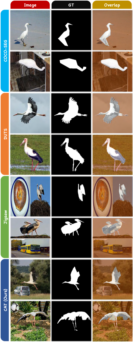
Figure 8: Comparison among different datasets. Semantic group: white stork.

Dataset Comparison

As mentioned in Sections 1 (Introduction) and 2 (Related Work) of the main body, current co-saliency detection models suffer from the inconsistency among training distribution $\mathcal{D}$, testing distribution $\mathcal{E}$, and true distribution $\mathcal{T}$. Although recent works (Fan et al. 2020; Zhang et al. 2020d) help $\mathcal{E}$ to move one-step closer towards $\mathcal{T}$, a dataset that can properly define $\mathcal{D}$ is still missing. Most works have to rely instead on semantic segmentation datasets (e.g., COCO-SEG (Wang et al. 2019) and COCO9213 (Lin et al. 2014)) and saliency detection datasets (e.g., DUTS (Wang et al. 2017)) for model training, which exacerbates the distribution gap.

Figures 8 and 9 show some typical examples from COCO-SEG (Wang et al. 2019), DUTS (Wang et al. 2017), Jigsaw (Zhang et al. 2020d), and our proposed dataset. Specifically, although there are rich contexts, the annotations of COCO-SEG (Wang et al. 2019) are coarse. Unlike pixel-by-pixel labeling, the annotations of COCO-SEG (Wang et al. 2019) are composed of polygons and triangles delimited by points. The fine-grained part of an object (e.g., the legs and tails of the while stork) and the object contours (e.g., the zebra behind shrubs and railings) cannot be appropriately depicted. In contrast, saliency detection datasets like DUTS (Wang et al. 2017) have sophisticated mask annotations. Parts such as the wingtip feathers and the slender legs of the white stork and the ears of the zebra are well-annotated. The reason why these examples are so different is that these two tasks have different purposes. While the former pays more attention to the segmentation of multiple objects in complex scenes, the latter emphasizes more on the high-precision detection of salient objects. However, the uni-object distribution of DUTS (Wang et al. 2017) is not in line with the objective of co-saliency detection (Fan et al. 2021a), i.e., to identify co-salient signals from multi-foreground visual contexts in a group-by-group manner.

Recent work (Zhang et al. 2020d) proposes to concatenate two images horizontally or vertically to form a multi-object jigsaw. This includes two resize processes: (1) resize candidate images to squares before concatenation; and (2) resize jigsawed images to squares before feeding into the network. Although this technique introduces co-salient signals, it also leads to severe distortion and incoherent concatenation boundaries. As shown in Figures 8 and 9, the jigsawed images become cluttered, and the objects in some examples (e.g., the zebra underneath the green apple and beside three dogs) are difficult to be recognized even by human eyes. This deviates from the original intention of co-saliency detection, i.e., to imitate human visual attentions (Jacobs, Goldman, and Shechtman 2010). On the contrary, the images in our dataset have clear visual contexts, carefully defined co-saliency, as well as high-quality annotations.

Data Collection

As mentioned in Section 3.2 (Group-Cut-Paste) of the main body, our GCP procedure leverages images from existing datasets for context adjustment. This means that the quality of the canvas determines the quality of the entire adjustment process. Therefore, we strictly followed the following criteria when selecting candidate images:

• Candidate images should have clear semantic meanings.

• Candidate images should have correct and sophisticated annotations.

Figures 10 and 11 show some discarded and passed cases (in terms of both image appearances and mask annotations). Specifically, we notice that there are cases that the key part of an object (e.g., the ears and nose of a cat) is missing or the corresponding mask annotation of an image is incorrect. This is because some samples in saliency detection datasets do not contain distinguished semantic information and thus treat all the regions in the foreground as salient and label them accordingly. Obviously, these examples do not meet our requirements, so we choose to pick them out of the candidate pool. Following the above criteria, we collected 8,375 candidate images with clear saliency (Fan et al. 2018a) and sophisticated annotations for further GCP processing.

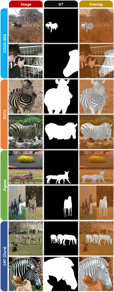
Figure 9: Comparison among different datasets. Semantic group: zebra.

More Superclass Details

As mentioned in Section 3.3 (Constructing the Dataset) of the main body, our dataset consists of 15 superclasses, i.e., aves, electronic product (elec.), food, fruit, insect, instrument (instru.), kitchenware (kitch.), mammal (mamm.), marine, other, reptile (rept.), sports, tool, transportation (trans.), and vegetable (vege.). Figure 14 shows the representative example of each superclass. It can be seen that our dataset is diverse in semantics, which covers a large number of categories. The superclass distribution is shown in the pie chart (see Figure 15) and tree chart (see Figure 16), respectively. Specifically, mammal occupies 73 of the 280 semantic groups (23$\%$), which is the largest among the 15 superclasses. The second-largest is the aves, which consists of 56 semantic groups (20$\%$). The remaining superclasses occupy a total of 54$\%$ subclasses, of which the smallest two are marine and vegetable, each containing four semantic groups. In general, the 15 superclasses in our dataset cover a large number of categories in different fields. We believe that such diversity and comprehensiveness can benefit future works in co-saliency detection and beyond.

More Subclass Details

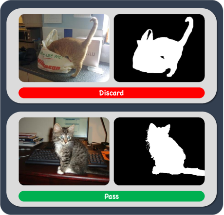
Figure 10: Data collection examples. Images with unclear/clear semantics are discarded/passed.

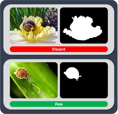
Figure 11: Data collection examples. Images with incorrect/correct annotations are discarded/passed.

As mentioned in Section 3.3 (Constructing the Dataset) of the main body, our dataset contains 280 subclasses (semantic groups), of which range from biological species and daily necessities. Specifically, as shown in Figure 17, each semantic group in our dataset is a collection of one specific species. These species usually have a uniform appearance, such as a specific shape, color, texture, etc. Thanks to the powerful pre-training model (Mahajan et al. 2018), these species are automatically classified to form diverse semantic groups. Figure 18 shows the distribution (w.r.t. the number of images per group) of all 280 semantic groups in CAT. The average number of images per group is 119.6. Among all the semantic groups, apple is the largest one with 824 images, while boston terrier and cell phone are the smallest, which contain 28 images. Such a distribution is in line with that of the recent evaluation datasets, i.e., CoSOD3k (Fan et al. 2020) and CoCA (Zhang et al. 2020d). The maximum/minimum numbers of images per group for these two datasets are 30/4 and 40/8, respectively. Another thing worth noting is the semantic hierarchy. Thanks to the abundant semantic information, our dataset offers diverse “semantic branches” (see Figure 13), which are similar to the “subtrees” of WordNet (Miller 1998).

Along the backbones of the “semantic tree”, such as dog, cat, and bird, our dataset has extended many “branches” that contain sophisticated species meanings. An example of the “branches” for dog is shown in Figure 19. Specifically, instead of regarding and aggregating every dog-related samples into a single group, we sincerely maintain their basic semantic hierarchy and divide them into different groups, i.e., golden retriever, staffordshire bull terrier, weimaraner, welsh springer spaniel, and yorkshire terrier. Our motives here are twofold. First of all, many current one-stage models rely too much on extracting high-level semantic information through pre-training and mapping this information into soft attention to achieve the extraction of co-salient signals. This solves the problem of “where to look” to a certain extent, but it is also restricted by the quality of pre-training and cannot make reasonable judgments about examples that have not been seen in the pre-training dataset. The second reason is that many potential application scenarios, such as online surveillance, have high requirements for the accuracy of identifying and distinguishing objects from the same roots. For example, continuously identifying the co-salient signal of a specific car from a surveillance video of the street scene requires the model to have the ability to distinguish it from other vehicles. Based on the above reasons, we construct these “semantic branches”. We hope that future models can consider both high-level semantic information and low-level appearance to achieve correct detection and segmentation of co-salient objects, especially those that have never been seen in the pre-training.

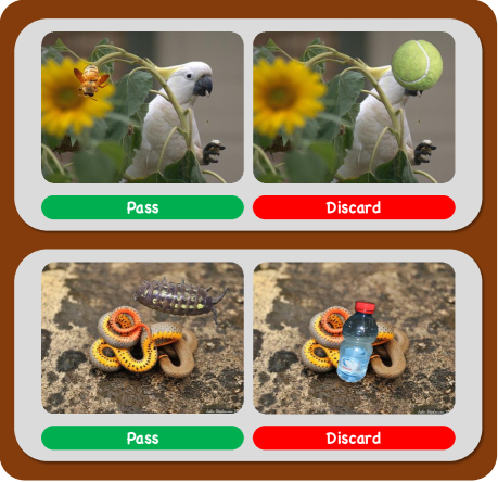
Figure 12: Quality control examples. Images with severe occlusions are discarded.

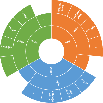
Figure 13: Examples of the “semantic branches” in our dataset. “lepid”: Lepidoptera; “testu”: Testudines; “prima”: Primates.

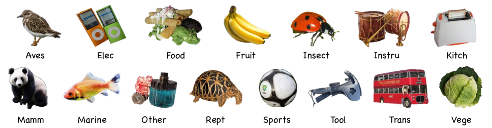
Figure 14: Representative example of each superclass in our dataset. Best viewed in color and zoomed-in for details.

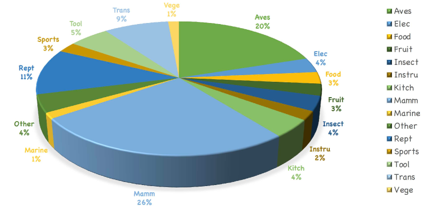
Figure 15: Pie chart for the superclass distribution of our dataset.

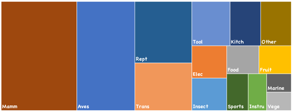
Figure 16: Tree chart for the superclass distribution of our dataset. The larger the area, the more semantic groups it contains.

Quality Control

As mentioned in Section 3.3 (Constructing the Dataset) of the main body, to ensure the high-quality of the dataset, we re-sampled some unsatisfactory examples (around 10$\%$). Here we give some examples of our selection criteria. As shown in Figure 12, objects with slender or meandering shapes, such as creatures like birds, centipedes, and snakes, and items like hammers, hatchets, and nails, can be occluded by objects pasted into the images, resulting in the loss of corresponding semantics. Therefore, we pick these examples out from the candidate pool and re-sample them via GCP.

Complete Group Patterns

As mentioned in Section 3.3 (Constructing the Dataset) of the main body, the patterns (calculated by averaging overlapping masks) of semantic groups in our dataset tend to have shape-biased appearances, which is consistent with the idea of saliency (Fan et al. 2018a). This is also the major difference between co-saliency detection (Fan et al. 2021a) and image co-segmentation (Liu and Duan. 2019). Here we show the complete group patterns for all 280 semantic groups in our dataset in Figures 20, 21, 22, and 23.

Summary

After supplementing more statistical and technical details, we hereby summarize the features of our dataset as follows.

• Scale. CAT aims to provide comprehensive coverage for co-saliency detection in the deep learning era. The current version of our dataset consists of 33,500 images with high-quality annotations, making it the largest specialized co-saliency detection dataset so far.

• Diversity. CAT organizes all image samples in a dense and diverse semantic hierarchy. Rooted from 15 superclasses, the 280 semantic groups in our dataset are like branches, which together construct a “data tree” covering a large number of categories.

• Uniqueness. CAT is constructed with the goal that images should have complex visual contexts with multiple foreground objects. To achieve this, we introduce the idea of counterfactual training and propose a GCP procedure to synthesize training samples without the need for labor-intensive pixel-level labeling.

• Quality. We would like to offer a clean dataset with diverse visual contexts and accurate annotations. Therefore, we have carefully considered the technical requirements in each step, formulated corresponding criteria, and strictly followed them. The experimental results also confirmed the reliability of our dataset.

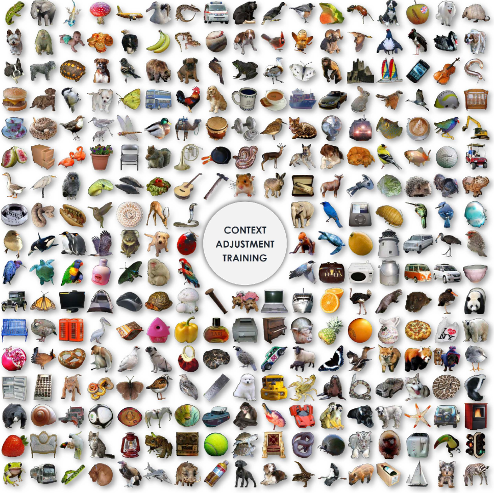
Figure 17: Representative example of each semantic group in our dataset. Best viewed in color and zoomed-in for details.

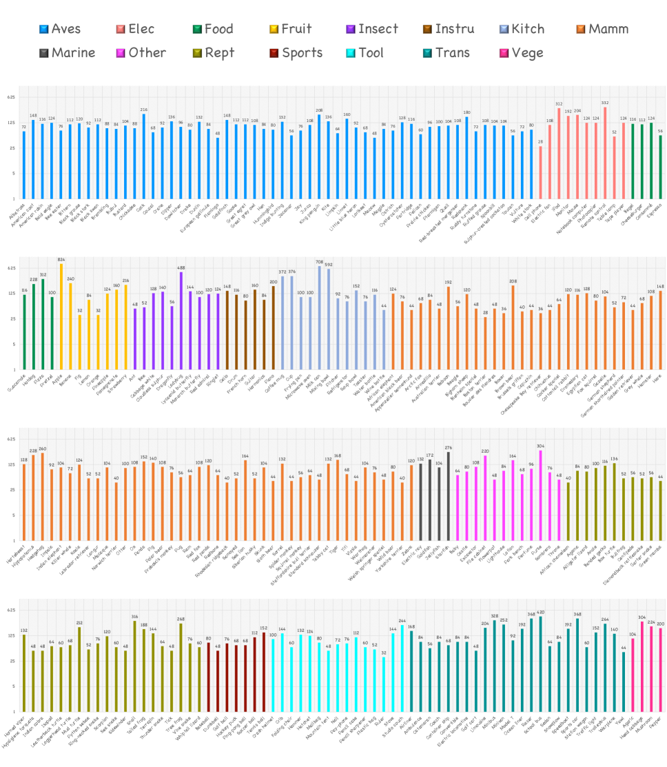
Figure 18: The distribution for the 280 semantic groups in CAT. Subclasses belong to the same superclass are highlighted with unified color. Best viewed in color and zoomed-in for details.

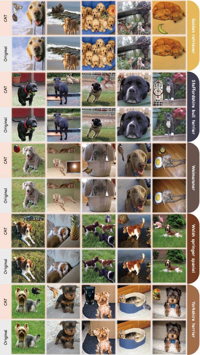
Figure 19: Examples of the “semantic branches” in our dataset. Best viewed in color and zoomed-in for details.

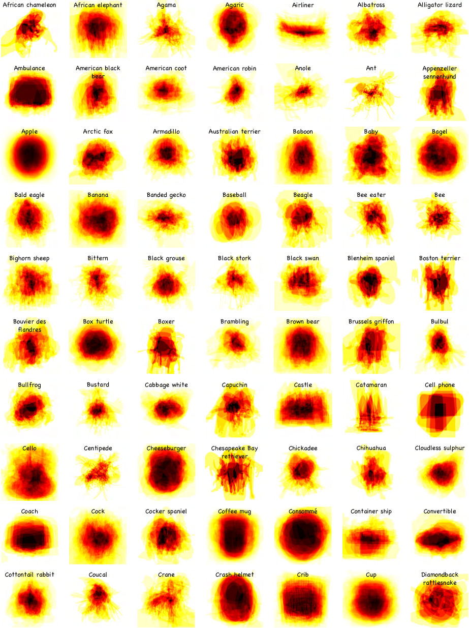
Figure 20: Patterns for the 280 groups in our dataset (1$\sim$70). Best viewed in color and zoomed-in for details.

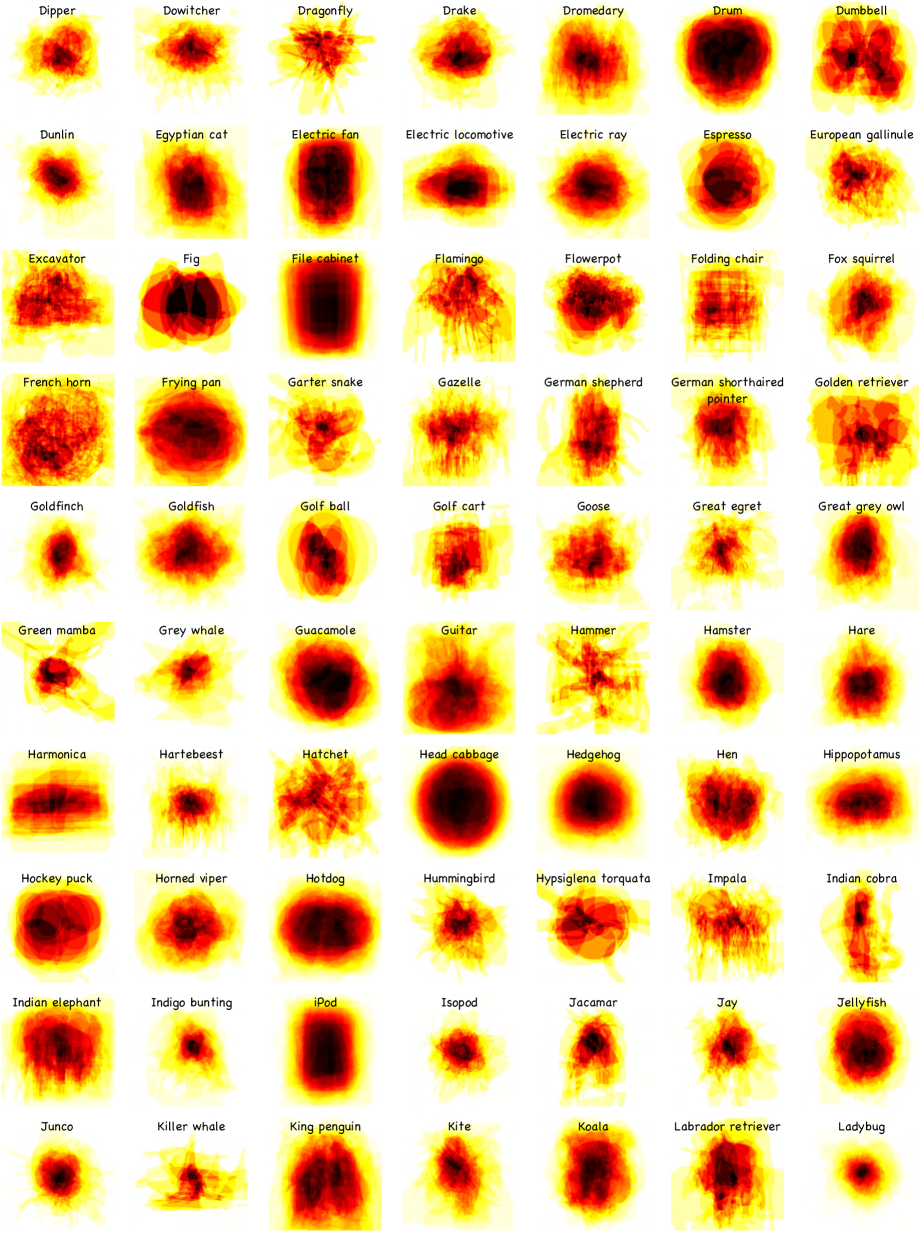
Figure 21: Patterns for the 280 groups in our dataset (71$\sim$140). Best viewed in color and zoomed-in for details.

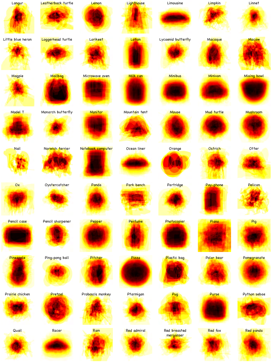
Figure 22: Patterns for the 280 groups in our dataset (141$\sim$210). Best viewed in color and zoomed-in for details.

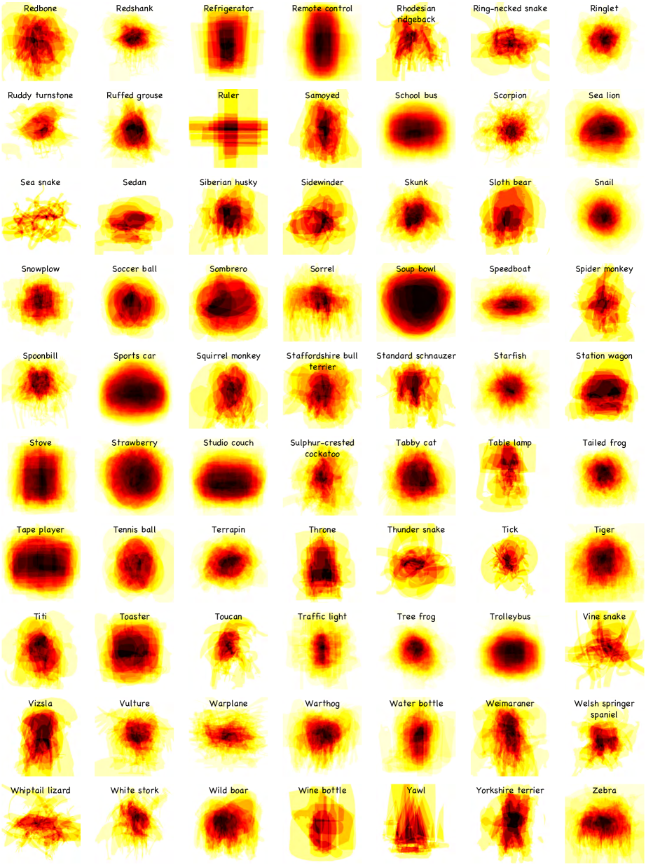
Figure 23: Patterns for the 280 groups in our dataset (211$\sim$280). Best viewed in color and zoomed-in for details.

Experimental Details

In this section, we further supplement some detailed information for our benchmark experiment and extensive qualitative results for a more comprehensive visual comparison.

Evaluation Metrics

As mentioned in Section 4.1 (Implementation Details) of the main body, we follow the convention by adopting the following four metrics to evaluate model performances in our benchmark experiment: mean absolute error (MAE) (Cheng et al. 2013), F-measure (Achanta et al. 2009), E-measure (Fan et al. 2018b), and structure measure ($S_{\alpha}$) (Fan et al. 2017). Denote $\mathcal{S}\in\mathbb{R}^{w\times h}$ and $\mathcal{G}\in\mathbb{R}^{w\times h}$ as the predicted saliency map and the ground-truth with width $w$ and height $h$, respectively. Here we further detail the characteristics of these metrics.

• Precision & Recall
  The basic building blocks for evaluations. Denote true-positive, true-negative, false-positive, and false-negative as TP, TN, FP, and FN, respectively. Precision ($\mathcal{P}$) and recall ($\mathcal{R}$) are calculated based on the binarized saliency map $\mathcal{S}$ and the ground-truth $\mathcal{G}$ as follows:

  $$\mathcal{P}=\frac{\textit{TP}}{\textit{TP}+\textit{FP}},~{}~{}~{}~{}~{}~{}~{}~{}\mathcal{R}=\frac{\textit{TP}}{\textit{TP}+\textit{FN}}.$$ (1)

• MAE (Cheng et al. 2013)
  Metric for measuring the average pixel-wise absolute error between saliency map $\mathcal{S}$ and ground-truth $\mathcal{G}$:

  $$\textit{MAE}=\frac{1}{w\times h}\sum_{i=1}^{w}\sum_{j=1}^{h}\mid\mathcal{S}(i,j)-\mathcal{G}(i,j)\mid,$$ (2)

  where $i$ and $j$ are the indexes.

• F-measure (Achanta et al. 2009)
  Metric for weighting precision ($\mathcal{P}$) and recall ($\mathcal{R}$), which is defined by the weighted harmonic mean as follows:

  $$F_{\beta}=\frac{(1+\beta^{2})\mathcal{P}\times\mathcal{R}}{\beta^{2}\mathcal{P}+\mathcal{R}},$$ (3)

  where coefficient $\beta^{2}$ is empirically set as $0.3$ to emphasize more on precision ($\mathcal{P}$) than recall ($\mathcal{R}$). Here we consider both the maximum value $F_{max}$ and the mean value $F_{avg}$, which is calculated by averaging the binarized saliency map $\mathcal{S}$ with an adaptive threshold.

• E-measure (Fan et al. 2018b)
  Metric for measuring both the pixel-level matching and the image-level statistics for the binarized saliency map $\mathcal{S}$, i.e.,

  $$Q_{\phi}=\frac{1}{w\times h}\sum_{i=1}^{w}\sum_{j=1}^{h}\phi(i,j),$$ (4)

  where $\phi$ denotes the enhanced alignment matrix (Fan et al. 2018b), which reflects the correlation between normalized saliency map $\mathcal{S}$ and ground-truth $\mathcal{G}$.

• Structure measure (Fan et al. 2017)
  Metric for measuring the structural similarity between saliency map $\mathcal{S}$ and ground-truth $\mathcal{G}$. Denote $S_{o}$ and $S_{r}$ as the object-aware similarity and the region-aware similarity (Fan et al. 2017), respectively. The structure measure is calculated as follows:

  $$S_{\alpha}=(1-\alpha)\times S_{o}+\alpha\times S_{r},$$ (5)

  where coefficient $\alpha$ is empirically set as $0.5$.

It worth noting that the aforementioned metrics are from saliency detection (Wang et al. 2021) and are widely adopted by co-saliency detection works (Fan et al. 2021a). Specifically, MAE (Cheng et al. 2013) and F-measure (Achanta et al. 2009) focus on measuring pixel-level errors, while E-measure (Fan et al. 2018b) and structure measure (Fan et al. 2017) consider structural similarities. Although F-measure (Achanta et al. 2009) fails to consider TN pixels, MAE (Cheng et al. 2013) makes up for this vacancy.

Overall, these metrics are complementary to each other. Together, they build a comprehensive assessment for evaluating model performances. However, so far there is no evaluation metric specifically designed for co-saliency detection. We hope that researchers in this area can design a suitable one that considers both co-saliency and group-wise effect in the near future.

Details of Loss Functions

As mentioned in Section 4.1 (Implementation Details) of the main body, we use five state-of-the-art models for the benchmark experiments, i.e., PoolNet (Liu et al. 2019), EGNet (Zhao et al. 2019), ICNet (Jin et al. 2020), GICD (Zhang et al. 2020d), and GCoNet (Fan et al. 2021b).

Specifically, PoolNet (Liu et al. 2019) adopts the standard binary cross-entropy loss for saliency detection and the balanced binary cross-entropy loss (Xie and Tu 2015) for edge detection. EGNet (Zhao et al. 2019) adopts the standard binary cross-entropy loss for both saliency detection and edge detection. ICNet (Jin et al. 2020) and GICD (Zhang et al. 2020d) adopt the IoU loss (Lin, Qi, and Jia 2019) and the soft IoU loss (Li, Chen, and Koltun 2018; Qin et al. 2019a) for co-saliency detection, respectively. For GCoNet (Fan et al. 2021b), three loss functions are aggregated, i.e., soft IoU loss (Li, Chen, and Koltun 2018; Qin et al. 2019a), focal loss (Lin et al. 2017), and cross-entropy loss. Several weights are applied to balance these three losses during training.

Details of Training Configurations

The detailed training configurations for models mentioned in Section 4.1 (Implementation Details) of the main body are summarized as follows.

• PoolNet (Liu et al. 2019)
  The Res2Net (Gao et al. 2021) version of PoolNet (Liu et al. 2019) is adopted in our experiments. The model is trained via the Adam optimizer (Kingma and Ba 2015) with learning rate $=4e-5$ and weight decay $=5e-4$. We run this model for 50 epochs and evaluate the checkpoints from the last three epochs.

• EGNet (Zhao et al. 2019)
  For this model, we adopt the one with the VGG backbone in our experiments. We follow the default setting by using the Adam optimizer (Kingma and Ba 2015) and assigning the learning rate as $2e-5$, weight decay as $5e-4$, and loss weight as $1$. Before the training, the edge maps for the training samples are prepared via the corresponding mask annotations of each dataset. We train EGNet (Zhao et al. 2019) for 30 epochs and divide the learning rate by 10 after 15 epochs. For each run, we evaluate the last three checkpoints of this model and report the average results.

• ICNet (Jin et al. 2020)
  For this model, we adopt both the VGG (Simonyan and Zisserman 2015) and ResNet (He et al. 2016) versions of EGNet (Zhao et al. 2019) to prepare the single-image-saliency-maps (SISMs). The Adam optimizer (Kingma and Ba 2015) with learning rate $=8e-6$ is adopted. In total, we run this model for 80 epochs and evaluate the checkpoints from the last three epochs.

• GICD (Zhang et al. 2020d)
  We keep the original training paradigm of GICD (Zhang et al. 2020d) in our experiments, which randomly selects at most 20 samples from each image group to extract the group saliency. Adam optimizer (Kingma and Ba 2015) is adopted. The initial learning rate is set as $2e-4$. We train this model for 100 epochs and reduce the learning to $80\%$ every 20 epochs. The CoSal2015 dataset (Zhang et al. 2016) is used as the validation set for picking the best possible checkpoints.

• GCoNet (Fan et al. 2021b)
  We adopt the default model architecture of GCoNet (Fan et al. 2021b), which is a VGG-based (Simonyan and Zisserman 2015) feature pyramid network. Similar to GICD (Zhang et al. 2020d), the group saliency is calculated by selecting and aggregating group samples. For each training episode, 16 samples from two different groups are picked. This model also uses the Adam optimizer (Kingma and Ba 2015) with learning rate $=2e-4$ and a total number of 50 epochs are trained. We use CoSal2015 (Zhang et al. 2016) as the validation set for picking the best possible checkpoints.

More Qualitative Results

In Section 4.3 (Qualitative Analysis) of the main body, we show some qualitative results of different training datasets on GICD (Zhang et al. 2020d). To offer a comprehensive and precise evaluation among different competitors, we show more visualization results here. The qualitative results for different datasets trained by ICNet (Jin et al. 2020) are shown in Figures 24, 25, 26, and 27. Furthermore, for EGNet (Zhao et al. 2019), the qualitative results are shown in Figures 28, 29, 30, and 31.

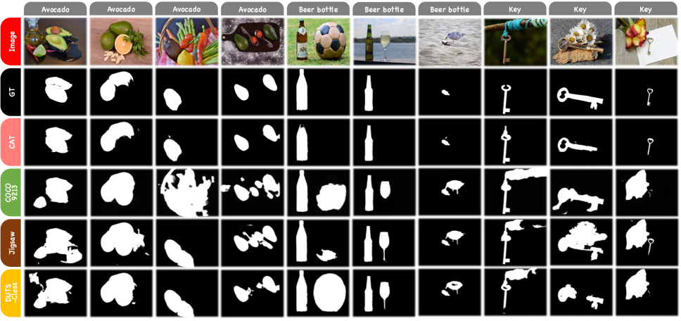
Figure 24: Qualitative comparison among different training datasets. Model: ICNet (Jin et al. 2020) (SISMs generated by pretrained EGNet with ResNet (He et al. 2016) backbone). Evaluation dataset: CoCA (Zhang et al. 2020d). Semantic groups from left to right: avocado, beer bottle, and key.

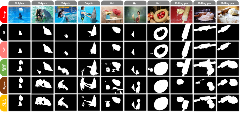
Figure 25: Qualitative comparison among different training datasets. Model: ICNet (Jin et al. 2020) (SISMs generated by pretrained EGNet with ResNet (He et al. 2016) backbone). Evaluation dataset: CoCA (Zhang et al. 2020d). Semantic groups from left to right: dolphin, hat, and rolling pin.

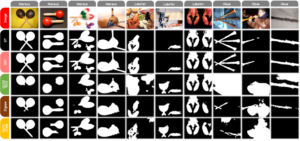
Figure 26: Qualitative comparison among different training datasets. Model: ICNet (Jin et al. 2020) (SISMs generated by pretrained EGNet with ResNet (He et al. 2016) backbone). Evaluation dataset: CoSOD3k (Fan et al. 2020). Semantic groups from left to right: maraca, lobster, and oboe.

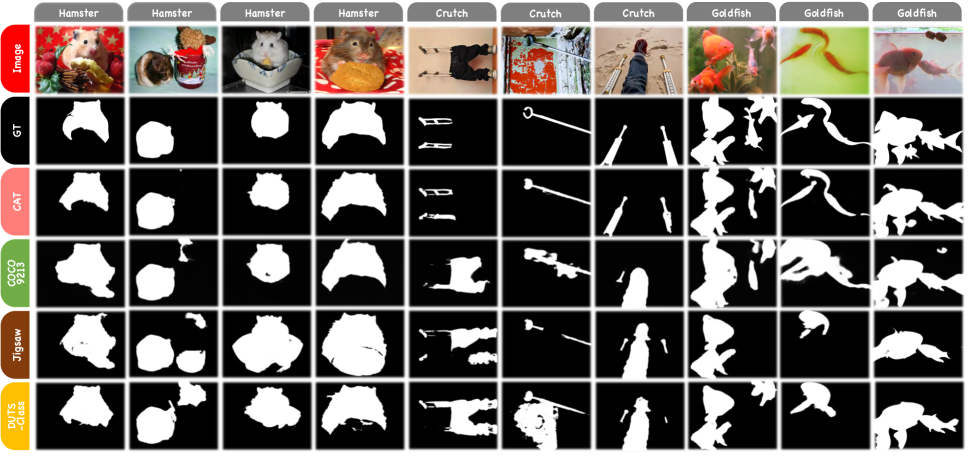
Figure 27: Qualitative comparison among different training datasets. Model: ICNet (Jin et al. 2020) (SISMs generated by pretrained EGNet with ResNet (He et al. 2016) backbone). Evaluation dataset: CoSOD3k (Fan et al. 2020). Semantic groups from left to right: hamster, crutch, and goldfish.

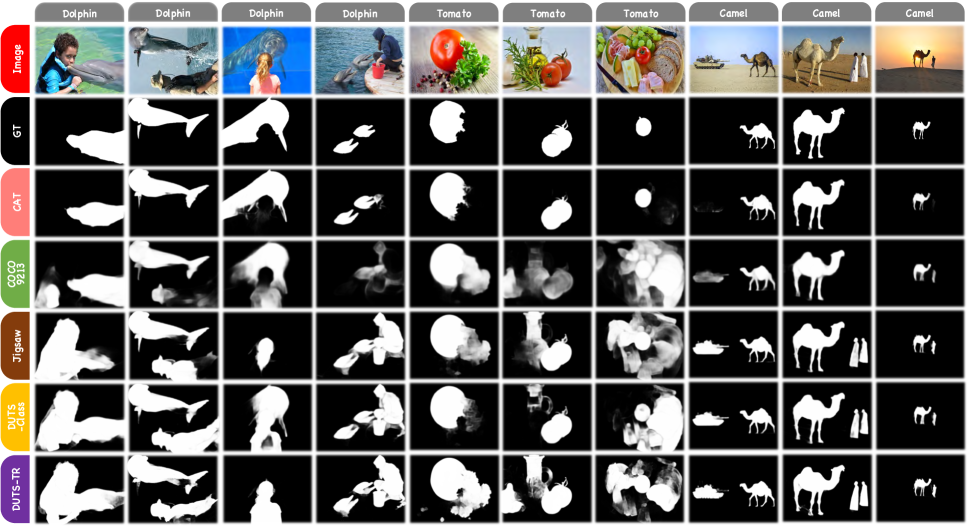
Figure 28: Qualitative comparison among different training datasets. Model: EGNet (Zhao et al. 2019). Evaluation dataset: CoCA (Zhang et al. 2020d). Semantic groups from left to right: dolphin, tomato, and camel.

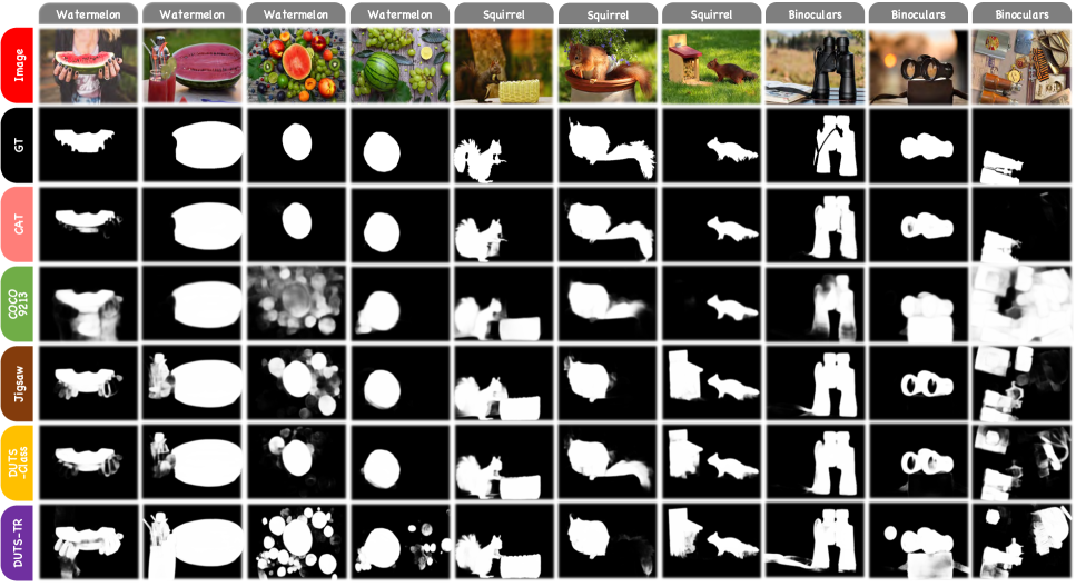
Figure 29: Qualitative comparison among different training datasets. Model: EGNet (Zhao et al. 2019). Evaluation dataset: CoCA (Zhang et al. 2020d). Semantic groups from left to right: watermelon, squirrel, and binoculars.

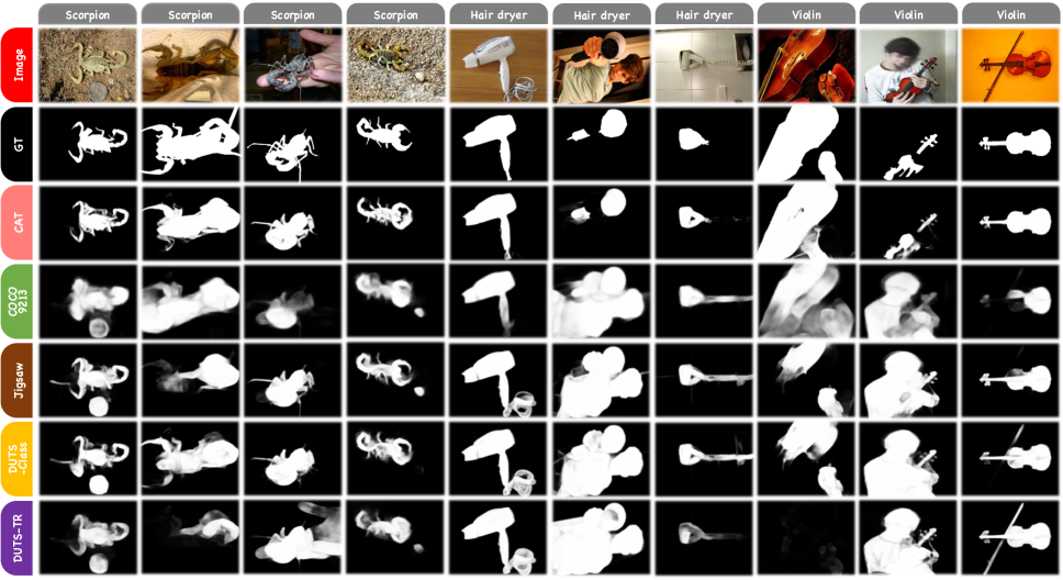
Figure 30: Qualitative comparison among different training datasets. Model: EGNet (Zhao et al. 2019). Evaluation dataset: CoSOD3k (Fan et al. 2020). Semantic groups from left to right: scorpion, hair dryer, and violin.

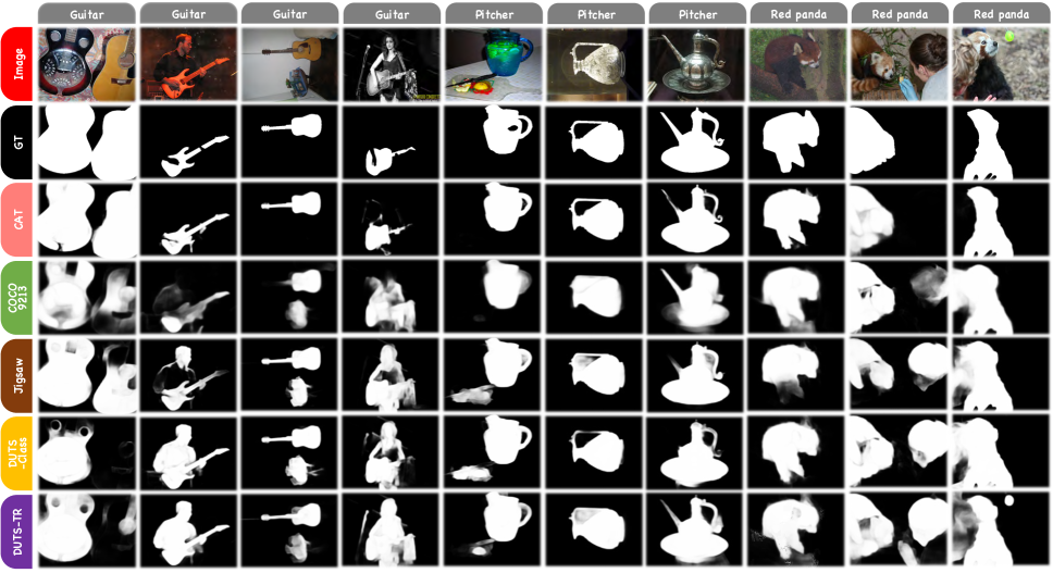
Figure 31: Qualitative comparison among different training datasets. Model: EGNet (Zhao et al. 2019). Evaluation dataset: CoSOD3k (Fan et al. 2020). Semantic groups from left to right: guitar, pitcher, and red panda.

Benchmark Study

In this section, to provide a more comprehensive benchmark study, we review the growth of co-saliency detection in chronological order and then discuss the corresponding works on datasets and models.

Chronology

Co-saliency detection is quite young compared to other conventional computer vision tasks like image classification and object detection, but more and more attention has been gained in recent years. As shown in Figure 32, there is a clear upward trend for research in co-saliency detection and its related fields.

Figure 34 shows the chronological structure of co-saliency detection. Specifically, Like most popular computer vision tasks, the evolution of co-saliency detection can be divided into two stages: traditional and modern. (Jacobs, Goldman, and Shechtman 2010) is the very beginning of this task. Since then, researchers have begun to pay attention to identify co-saliency signals in images groups. Traditional works (Chen 2010; Fu, Cao, and Tu 2013; Li, Meng, and Ngan 2013; Liu et al. 2014) depend on certain heuristics like the color contrast and background prior to extract intra-image and inter-image cues, while modern methods (Zhang et al. 2015; Yao et al. 2017; Cong et al. 2017) mainly adopt variant network structures to learn patterns from data, such as convolutional neural networks (ju Jeong, Hwang, and Cho 2018; Zhang et al. 2019, 2020d; Jin et al. 2020; Fan et al. 2021a, b), recurrent neural networks (Li et al. 2019a), graph neural networks (Zhang et al. 2020b), and generative adversarial networks (Qian et al. 2021).

Dataset Zoo

In Section 2 (Related Work) of the main body, we give a comprehensive analysis for the 10 training datasets in co-saliency detection. Here we adopt a similar procedure and show the characteristics of the datasets used to evaluate model performances, i.e., MSRC (Winn, Criminisi, and Minka 2005), iCoseg (Batra et al. 2010), ImagePair (Li and Ngan 2011), CoSal2015 (Zhang et al. 2016), WISD (Yue et al. 2019), COCO-SEG-Val (Wang et al. 2019), CoSOD3k (Fan et al. 2020), and CoCA (Zhang et al. 2020d). The statistics of these evaluation datasets are shown in Table 9 and Figure 33.

Specifically, small-scale datasets like MSRC (Winn, Criminisi, and Minka 2005) and iCoseg (Batra et al. 2010) are popular among works from early years only. COCO-SEG-Val (Wang et al. 2019) is the largest one among all nine datasets, which contains 8,662 images from 78 categories. However, as we mentioned before, the mask annotations for semantic segmentation datasets like COCO-SEG (Wang et al. 2019) are coarse compared with both saliency and co-saliency detection datasets; thus, it may not be accurate enough for model evaluations. CoSal2015 (Zhang et al. 2016) is a more reliable choice in recent years and has been adopted as both the training and evaluation dataset for different works. However, the context and diversity of this dataset are getting insufficient with the deepening of related research. Recent works (Fan et al. 2021b, a) have achieved nearly 0.85 in F-measure and structure measure and 0.9 in E-measure on CoSal2015 (Zhang et al. 2016). The two datasets proposed last year (i.e., CoSOD3k (Fan et al. 2020) and CoCA (Zhang et al. 2020d)) improved the quality of visual contexts, increased the dataset scales, and introduced more diversity. Therefore, we adopt them in our benchmark experiment to evaluate performances.

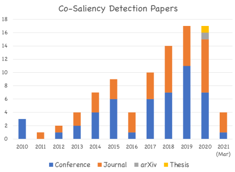
Figure 32: The number of co-saliency detection related papers published each year.

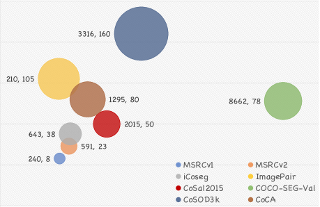
Figure 33: Bubble chart for evaluation datasets. Horizontal axis: number of images; Vertical axis: number of groups. The bigger the bubble, the more semantic groups it contains.

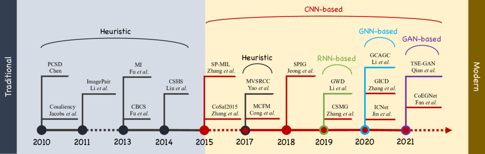
Figure 34: The chronology of co-saliency detection. Representative works for each year are listed and divided by types.

#	Dataset	Year	#Img.	#Cat.	#Avg.	#Max.	#Min.	Mul.	Sal.	Larg.	H.Q.	Inputs
1	MSRCv1	2005	240	8	30.0	30	30	✗	✓	✗	✗	Group images
2	MSRCv2	2005	591	23	25.7	34	21	✗	✓	✗	✗	Group images
3	iCoseg	2010	643	38	16.9	41	4	✗	✓	✗	✓	Group images
4	ImagePair	2011	210	105	2.0	2	2	✗	✓	✗	✗	Pair images
5	CoSal2015	2015	2,015	50	40.3	52	26	✓	✓	✓	✓	Group images
6	WISD	2019	2,019	-	-	-	-	✓	-	✓	-	Group images
7	COCO-SEG-Val	2019	8,662	78	111.1	2,107	6	✓	✗	✓	✗	Group images
8	CoSOD3k	2020	3,316	160	20.7	30	4	✓	✓	✓	✓	Group images
9	CoCA	2020	1,295	80	16.2	40	8	✓	✓	✓	✓	Group images

Table 9: Datasets used for evaluating co-saliency detection models. #Img.: Number of images; #Cat.: Number of categories; #Avg.: Average number of images per category; #Max.: Maximum number of images per group; #Min.: Minimum number of images per group. Mul.: Whether contains multiple foreground objects or not; Sal.: Whether maintains saliency or not; Larg.: Whether large-scale (more than 1k images) or not; H.Q.: Whether has high-quality annotations or not. “-” denotes “not available”.

#	Model	Venue	MAE $\downarrow$	$F_{max}$ $\uparrow$	$F_{avg}$ $\uparrow$	$E_{max}$ $\uparrow$	$E_{avg}$ $\uparrow$	$S_{\alpha}$ $\uparrow$
1	CBCS (Fu, Cao, and Tu 2013)	TIP’13	0.228	0.468	0.322	0.633	0.509	0.529
2	CSHS (Liu et al. 2014)	SPL’14	0.309	0.484	-	0.656	-	0.563
3	ESMG (Li et al. 2014)	SPL’14	0.239	0.364	-	-	0.615	0.532
4	CODR (Ye et al. 2015)	SPL’15	0.229	0.458	-	-	0.645	0.630
5	GW (Wei et al. 2017)	IJCAI’17	0.147	0.649	-	0.777	-	0.716
6	PoolNet (Liu et al. 2019)	CVPR’19	0.171	0.561	0.528	0.751	0.689	0.636
7	CSMG (Zhang et al. 2019)	CVPR’19	0.141	0.729	0.596	0.821	0.675	0.727
8	BASNet (Qin et al. 2019b)	CVPR’19	0.122	0.696	-	-	0.791	0.753
9	EGNet★ (Zhao et al. 2019)	ICCV’19	0.088	0.745	0.735	0.840	0.830	0.791
10	SCRN (Wu, Su, and Huang 2019)	ICCV’19	0.118	0.717	-	-	0.806	0.773
11	RCAN (Li et al. 2019b)	IJCAI’19	0.130	0.688	-	0.808	-	0.744
12	SSNM (Zhang et al. 2020a)	AAAI’20	0.120	0.675	-	-	0.756	0.726
13	F3Net (Wei, Wang, and Huang 2020)	AAAI’20	0.114	0.717	-	0.802	-	0.772
14	GCAGC (Zhang et al. 2020b)	CVPR’20	0.100	0.740	-	-	0.831	0.778
15	MINet (Pang et al. 2020)	CVPR’20	0.122	0.707	-	0.782	-	0.754
16	ICNet-V★ (Jin et al. 2020)	NeurIPS’20	0.068	0.791	0.782	0.870	0.866	0.811
17	ICNet-R★ (Jin et al. 2020)	NeurIPS’20	0.067	0.792	0.783	0.872	0.867	0.817
18	CoADNet (Zhang et al. 2020c)	NeurIPS’20	0.078	0.786	-	0.874	-	0.822
19	GICD★ (Zhang et al. 2020d)	ECCV’20	0.070	0.786	0.779	0.886	0.863	0.812
20	CoEGNet (Fan et al. 2021a)	TPAMI’21	0.092	0.736	-	0.825	-	0.762
21	DeepACG (Zhang et al. 2021)	CVPR’21	0.089	0.756	-	-	0.838	0.792
22	GCoNet★ (Fan et al. 2021b)	CVPR’21	0.065	0.789	0.784	0.865	0.862	0.813

Table 10: Benchmarking results on CoSOD3k (Fan et al. 2020). Symbols $\uparrow$ and $\downarrow$ denote the metrics which are the higher and the lower the better, respectively. Models trained by our CAT are highlighted with superscript ${\bigstar}$. “-V” and “-R” denote models with VGG and ResNet backbones, respectively. The best, second best, and third best results for each metric are highlighted with red, blue, and orange colors.

#	Model	Venue	MAE $\downarrow$	$F_{max}$ $\uparrow$	$F_{avg}$ $\uparrow$	$E_{max}$ $\uparrow$	$E_{avg}$ $\uparrow$	$S_{\alpha}$ $\uparrow$
1	CBCS (Fu, Cao, and Tu 2013)	TIP’13	0.180	0.313	0.230	0.641	0.531	0.523
2	CSHS (Liu et al. 2014)	SPL’14	-	-	-	-	-	-
3	ESMG (Li et al. 2014)	SPL’14	-	-	-	-	-	-
4	CODR (Ye et al. 2015)	SPL’15	-	-	-	-	-	-
5	GW (Wei et al. 2017)	IJCAI’17	0.166	0.408	-	0.701	-	0.602
6	PoolNet (Liu et al. 2019)	CVPR’19	0.181	0.346	0.323	0.707	0.625	0.561
7	CSMG (Zhang et al. 2019)	CVPR’19	0.124	0.508	-	0.735	-	0.632
8	BASNet (Qin et al. 2019b)	CVPR’19	0.195	0.397	-	-	0.623	0.589
9	EGNet★ (Zhao et al. 2019)	ICCV’19	0.143	0.449	0.439	0.691	0.678	0.626
10	SCRN (Wu, Su, and Huang 2019)	ICCV’19	0.166	0.416	-	-	0.658	0.610
11	RCAN (Li et al. 2019b)	IJCAI’19	0.160	0.422	-	0.702	-	0.616
12	SSNM (Zhang et al. 2020a)	AAAI’20	0.116	0.482	-	-	0.741	0.628
13	F3Net (Wei, Wang, and Huang 2020)	AAAI’20	0.178	0.437	-	0.678	-	0.614
14	GCAGC (Zhang et al. 2020b)	CVPR’20	0.111	0.523	-	-	0.754	0.669
15	MINet (Pang et al. 2020)	CVPR’20	0.221	0.387	-	0.634	-	0.550
16	ICNet-V★ (Jin et al. 2020)	NeurIPS’20	0.108	0.529	0.522	0.744	0.734	0.673
17	ICNet-R★ (Jin et al. 2020)	NeurIPS’20	0.101	0.533	0.526	0.751	0.743	0.678
18	CoADNet (Zhang et al. 2020c)	NeurIPS’20	-	-	-	-	-	-
19	GICD★ (Zhang et al. 2020d)	ECCV’20	0.116	0.523	0.516	0.727	0.716	0.668
20	CoEGNet (Fan et al. 2021a)	TPAMI’21	0.104	0.499	-	0.717	-	0.616
21	DeepACG (Zhang et al. 2021)	CVPR’21	0.102	0.552	-	-	0.771	0.688
22	GCoNet★ (Fan et al. 2021b)	CVPR’21	0.089	0.531	0.528	0.730	0.728	0.673

Table 11: Benchmarking results on CoCA (Zhang et al. 2020d). Symbols $\uparrow$ and $\downarrow$ denote the metrics which are the higher and the lower the better, respectively. Models trained by our CAT are highlighted with superscript ${\bigstar}$. “-V” and “-R” denote models with VGG and ResNet backbones, respectively. The best, second best, and third best results for each metric are highlighted with red, blue, and orange colors.

Model Zoo

In Section 4 (Benchmark Experiment) of the main body, we have evaluated five state-of-the-art co-saliency detection models in the benchmark experiment part of the main body, i.e., PoolNet (Liu et al. 2019), EGNet (Zhao et al. 2019), ICNet (Jin et al. 2020), GICD (Zhang et al. 2020d), and GCoNet (Fan et al. 2021b). A more comprehensive benchmarking study of 22 models are shown in Tables 10 and 11. For the continuous growth of this task, we will keep updating the evaluation results of more models to the benchmark.

References

- Achanta et al. (2009) Achanta, R.; Hemami, S.; Estrada, F.; and Susstrunk, S. 2009. Frequency-Tuned Salient Region Detection. CVPR, 1597–1604.
- Batra et al. (2010) Batra, D.; Kowdle, A.; Parikh, D.; Luo, J.; and Chen, T. 2010. iCoseg: Interactive Co-Segmentation with Intelligent Scribble Guidance. CVPR, 3169–3176.
- Borji et al. (2019) Borji, A.; Cheng, M.-M.; Hou, Q.; Jiang, H.; and Li, J. 2019. Salient Object Detection: A Survey. Comp. Visual Media, 5(2): 117–150.
- Chen (2010) Chen, H.-T. 2010. Preattentive Co-Saliency Detection. ICIP, 1117–1120.
- Chen et al. (2020) Chen, L.; Yan, X.; Xiao, J.; Zhang, H.; Pu, S.; and Zhuang, Y. 2020. Counterfactual Samples Synthesizing for Robust Visual Question Answering. CVPR, 10800–10809.
- Cheng et al. (2014a) Cheng, M.-M.; Mitra, N. J.; Huang, X.; and Hu, S.-M. 2014a. Salientshape: Group Saliency in Image Collections. Vis. Comput., 30(4): 443–453.
- Cheng et al. (2014b) Cheng, M.-M.; Mitra, N. J.; Huang, X.; Torr, P. H.; and Hu, S.-M. 2014b. Global contrast based salient region detection. IEEE Trans. Pattern Anal. Mach. Intell., 37(3): 569–582.
- Cheng et al. (2013) Cheng, M.-M.; Warrell, J.; Lin, W.-Y.; Zheng, S.; Vineet, V.; and Crook, N. 2013. Efficient Salient Region Detection with Soft Image Abstraction. ICCV, 1529–1536.
- Cong et al. (2017) Cong, R.; Lei, J.; Fu, H.; Huang, Q.; Cao, X.; and Hou, C. 2017. Co-Saliency Detection for RGBD Images based on Multi-Constraint Feature Matching and Cross Label Propagation. IEEE Trans. Image Process., 27(2): 568–579.
- Cubuk et al. (2019) Cubuk, E. D.; Zoph, B.; Mane, D.; Vasudevan, V.; and Le, Q. V. 2019. Autoaugment: Learning augmentation strategies from data. CVPR, 113–123.
- Dai et al. (2013) Dai, J.; Wu, Y. N.; Zhou, J.; and Zhu, S.-C. 2013. Cosegmentation and cosketch by unsupervised learning. ICCV, 1305–1312.
- Deng et al. (2009) Deng, J.; Dong, W.; Socher, R.; Li, L.-J.; Li, K.; and Fei-Fei, L. 2009. ImageNet: A Large-Scale Hierarchical Image Database. CVPR, 248–255.
- DeVries and Taylor (2017) DeVries, T.; and Taylor, G. W. 2017. Improved Regularization of Convolutional Neural Networks with Cutout. arXiv preprint arXiv:1708.04552.
- Divvala et al. (2009) Divvala, S. K.; Hoiem, D.; Hays, J. H.; Efros, A. A.; and Hebert, M. 2009. An Empirical Study of Context in Object Detection. CVPR, 1271–1278.
- Dwibedi, Misra, and Hebert (2017) Dwibedi, D.; Misra, I.; and Hebert, M. 2017. Cut, Paste and Learn: Surprisingly Easy Synthesis for Instance Detection. ICCV, 1301–1310.
- Fan et al. (2018a) Fan, D.-P.; Cheng, M.-M.; Liu, J.-J.; Gao, S.-H.; Hou, Q.; and Borji, A. 2018a. Salient Objects in Clutter: Bringing Salient Object Detection to the Foreground. ECCV, 186–202.
- Fan et al. (2017) Fan, D.-P.; Cheng, M.-M.; Liu, Y.; Li, T.; and Borji, A. 2017. Structure-Measure: A New Way to Evaluate Foreground Maps. ICCV, 4548–4557.
- Fan et al. (2018b) Fan, D.-P.; Gong, C.; Cao, Y.; Ren, B.; Cheng, M.-M.; and Borji, A. 2018b. Enhanced-Alignment Measure for Binary Foreground Map Evaluation. IJCAI.
- Fan et al. (2021a) Fan, D.-P.; Li, T.; Lin, Z.; Ji, G.-P.; Zhang, D.; Cheng, M.-M.; Fu, H.; and Shen, J. 2021a. Re-thinking Co-Salient Object Detection. IEEE Trans. Pattern Anal. Mach. Intell.
- Fan et al. (2020) Fan, D.-P.; Lin, Z.; Ji, G.-P.; Zhang, D.; Fu, H.; and Cheng, M.-M. 2020. Taking a Deeper Look at Co-Salient Object Detection. CVPR, 2919–2929.
- Fan et al. (2021b) Fan, Q.; Fan, D.-P.; Fu, H.; Tang, C.-K.; Shao, L.; and Tai, Y.-W. 2021b. Group Collaborative Learning for Co-Salient Object Detection. CVPR, 12288–12298.
- Fu, Cao, and Tu (2013) Fu, H.; Cao, X.; and Tu, Z. 2013. Cluster-based Co-Saliency Detection. IEEE Trans. Image Process., 22(10): 3766–3778.
- Gao et al. (2021) Gao, S.; Cheng, M.-M.; Zhao, K.; Zhang, X.-Y.; Yang, M.-H.; and Torr, P. H. 2021. Res2Net: A New Multi-Scale Backbone Architecture. IEEE Trans. Pattern Anal. Mach. Intell., 43(2): 652–662.
- Gao et al. (2020) Gao, Z.; Xu, C.; Zhang, H.; Li, S.; and de Albuquerque, V. H. C. 2020. Trustful Internet of Surveillance Things based on Deeply Represented Visual Co-Saliency Detection. IEEE Internet Things J., 7(5): 4092–4100.
- He et al. (2016) He, K.; Zhang, X.; Ren, S.; and Sun, J. 2016. Deep Residual Learning for Image Recognition. CVPR, 770–778.
- Hendrycks et al. (2020) Hendrycks, D.; Mu, N.; Cubuk, E. D.; Zoph, B.; Gilmer, J.; and Lakshminarayanan, B. 2020. Augmix: A Simple Data Processing Method to Improve Robustness and Uncertainty. ICLR.
- Herranz, Jiang, and Li (2016) Herranz, L.; Jiang, S.; and Li, X. 2016. Scene Recognition with CNNs: Objects, Scales and Dataset Bias. CVPR, 571–579.
- Jacobs, Goldman, and Shechtman (2010) Jacobs, D. E.; Goldman, D. B.; and Shechtman, E. 2010. Cosaliency: Where People Look when Comparing Images. UIST, 219–228.
- Jerripothula, Cai, and Yuan (2016) Jerripothula, K. R.; Cai, J.; and Yuan, J. 2016. CATS: Co-Saliency Activated Tracklet Selection for Video Co-localization. ECCV, 187–202.
- Jerripothula, Cai, and Yuan (2019) Jerripothula, K. R.; Cai, J.; and Yuan, J. 2019. Efficient Video Object Co-Localization With Co-Saliency Activated Tracklets. IEEE Trans. Circuits Syst. Video Technol., 29(3): 744–755.
- Jin et al. (2020) Jin, W.-D.; Xu, J.; Cheng, M.-M.; Zhang, Y.; and Guo, W. 2020. ICNet: Intra-Saliency Correlation Network for Co-Saliency Detection. NeurIPS.
- ju Jeong, Hwang, and Cho (2018) ju Jeong, D.; Hwang, I.; and Cho, N. I. 2018. Co-Salient Object Detection based on Deep Saliency Networks and Seed Propagation over an Integrated Graph. IEEE Trans. Image Process., 27(12): 5866–5879.
- Kingma and Ba (2015) Kingma, D. P.; and Ba, J. 2015. Adam: A Method for Stochastic Optimization. ICLR.
- Krähenbühl and Koltun (2011) Krähenbühl, P.; and Koltun, V. 2011. Efficient Inference in Fully Connected CRFs with Gaussian Edge Potentials. NeurIPS.
- LeCun et al. (1998) LeCun, Y.; Bottou, L.; Bengio, Y.; and Haffner, P. 1998. Gradient-based Learning Applied to Document Recognition. Proc. IEEE, 86(11): 2278–2324.
- Li et al. (2019a) Li, B.; Sun, Z.; Li, Q.; Wu, Y.; and Hu, A. 2019a. Group-Wise Deep Object Co-Segmentation with Co-Attention Recurrent Neural Network. ICCV, 8519–8528.
- Li et al. (2019b) Li, B.; Sun, Z.; Tang, L.; Sun, Y.; and Shi, J. 2019b. Detecting Robust Co-Saliency with Recurrent Co-Attention Neural Network. IJCAI.
- Li, Meng, and Ngan (2013) Li, H.; Meng, F.; and Ngan, K. N. 2013. Co-Salient Object Detection From Multiple Images. IEEE Trans. Multimedia, 15(8): 1896–1909.
- Li and Ngan (2011) Li, H.; and Ngan, K. N. 2011. A Co-Saliency Model of Image Pairs. IEEE Trans. Image Process., 20(12): 3365–3375.
- Li et al. (2014) Li, Y.; Fu, K.; Liu, Z.; and Yang, J. 2014. Efficient saliency-model-guided visual co-saliency detection. IEEE Signal Processing Letters, 7264–7273.
- Li, Chen, and Koltun (2018) Li, Z.; Chen, Q.; and Koltun, V. 2018. Interactive Image Segmentation with Latent Diversity. CVPR.
- Lin, Qi, and Jia (2019) Lin, H.; Qi, X.; and Jia, J. 2019. AGSS-VOS: Attention Guided Single-Shot Video Object Segmentation. ICCV.
- Lin et al. (2017) Lin, T.-Y.; Goyal, P.; Girshick, R.; He, K.; and Dollár, P. 2017. Focal loss for dense object detection. ICCV, 2980–2988.
- Lin et al. (2014) Lin, T.-Y.; Maire, M.; Belongie, S.; Hays, J.; Perona, P.; Ramanan, D.; Dollár, P.; and Zitnick, C. L. 2014. Microsoft COCO: Common Objects in Context. ECCV, 740–755.
- Liu et al. (2019) Liu, J.-J.; Hou, Q.; Cheng, M.-M.; Feng, J.; and Jiang, J. 2019. A Simple Pooling-based Design for Real-Time Salient Object Detection. CVPR, 3917–3926.
- Liu and Duan. (2019) Liu, X.; and Duan., X. 2019. Automatic Image Co-Segmentation: A Survey. arXiv preprint arXiv:1911.07685.
- Liu et al. (2014) Liu, Z.; Zou, W.; Li, L.; Shen, L.; and Meur, O. L. 2014. Co-Saliency Detection based on Hierarchical Segmentation. IEEE Signal Process. Lett., 21(1): 88–92.
- Mahajan et al. (2018) Mahajan, D.; Girshick, R.; Ramanathan, V.; He, K.; Paluri, M.; Li, Y.; Bharambe, A.; and Maaten, L. V. D. 2018. Exploring the Limits of Weakly Supervised Pretraining. ECCV, 181–196.
- Miller (1998) Miller, G. A. 1998. WordNet: An Electronic Lexical Database. MIT Press.
- Niu et al. (2021) Niu, Y.; Tang, K.; Zhang, H.; Lu, Z.; Hua, X.-S.; and Wen, J.-R. 2021. Counterfactual VQA: A Cause-Effect Look at Language Bias. CVPR, 12700–12710.
- Pang et al. (2020) Pang, Y.; Zhao, X.; Zhang, L.; and Lu, H. 2020. Multi-scale interactive network for salient object detection. CVPR.
- Pearl (2009) Pearl, J. 2009. Causality. Cambridge University Press.
- Pearl (2013) Pearl, J. 2013. Direct and Indirect Effects. arXiv preprint arXiv:1301.2300.
- Pearl, Glymour, and Jewell (2016) Pearl, J.; Glymour, M.; and Jewell, N. P. 2016. Causal Inference in Statistics: A Primer. John Wiley & Sons.
- Pearl and Mackenzie (2018) Pearl, J.; and Mackenzie, D. 2018. The Book of Why: The New Science of Cause and Effect. Basic Books.
- Qian et al. (2021) Qian, X.; Cheng, X.; Cheng, G.; Yao, X.; and Jiang, L. 2021. Two-Stream Encoder GAN With Progressive Training for Co-Saliency Detection. IEEE Signal Process. Lett., 28: 180–184.
- Qin et al. (2019a) Qin, X.; Zhang, Z.; Huang, C.; Gao, C.; Dehghan, M.; and Jagersand, M. 2019a. BASNet: Boundary-Aware Salient Object Detection. CVPR.
- Qin et al. (2019b) Qin, X.; Zhang, Z.; Huang, C.; Gao, C.; and Jagersand, M. 2019b. Basnet: Boundary-aware salient object detection. CVPR.
- Simonyan and Zisserman (2015) Simonyan, K.; and Zisserman, A. 2015. Very Deep Convolutional Networks for Large-Scale Image Recognition. ICLR.
- Suzuki (1985) Suzuki, S. 1985. Topological Structural Analysis of Digitized Binary Images by Border Following. Comput. Vis. Graphics Image Process., 30(1): 32–46.
- Tang, Huang, and Zhang (2020) Tang, K.; Huang, J.; and Zhang, H. 2020. Long-Tailed Classification by Keeping the Good and Removing the Bad Momentum Causal Effect. NeurIPS.
- Torralba and Efros (2011) Torralba, A.; and Efros, A. A. 2011. Unbiased Look at Dataset Bias. CVPR, 1521–1528.
- Wang et al. (2019) Wang, C.; Zha, Z.-J.; Liu, D.; and Xie, H. 2019. Robust Deep Co-Saliency Detection with Group Semantic. AAAI, 8917–8924.
- Wang et al. (2017) Wang, L.; Lu, H.; Wang, Y.; Feng, M.; Wang, D.; Yin, B.; and Ruan, X. 2017. Learning to Detect Salient Objects with Image-Level Supervision. CVPR, 136–145.
- Wang et al. (2020) Wang, T.; Huang, J.; Zhang, H.; and Sun, Q. 2020. Visual Commonsense R-CNN. CVPR, 10760–10770.
- Wang et al. (2021) Wang, W.; Lai, Q.; Fu, H.; Shen, J.; Ling, H.; and Yang, R. 2021. Salient Object Detection in the Deep Learning Era: An In-Depth Survey. IEEE Trans. Pattern Anal. Mach. Intell.
- Wei, Wang, and Huang (2020) Wei, J.; Wang, S.; and Huang, Q. 2020. F3Net: Fusion, feedback and focus for salient object detection. AAAI.
- Wei et al. (2017) Wei, L.; Zhao, S.; Bourahla, O. E. F.; Li, X.; and Wu, F. 2017. Group-Wise Deep Co-Saliency Detection. IJCAI.
- Winn, Criminisi, and Minka (2005) Winn, J.; Criminisi, A.; and Minka, T. 2005. Object Categorization by Learned Universal Visual Dictionary. ICCV, 1800–1807.
- Wu, Su, and Huang (2019) Wu, Z.; Su, L.; and Huang, Q. 2019. Stacked cross refinement network for edge-aware salient object detection. ICCV, 7264–7273.
- Xie and Tu (2015) Xie, S.; and Tu, Z. 2015. Holistically-Nested Edge Detection. ICCV.
- Yang et al. (2013) Yang, C.; Zhang, L.; Lu, H.; Ruan, X.; and Yang, M.-H. 2013. Saliency detection via graph-based manifold ranking. CVPR, 3166–3173.
- Yao et al. (2017) Yao, X.; Han, J.; Zhang, D.; and Nie, F. 2017. Revisiting Co-Saliency Detection: A Novel Approach based on Two-Stage Multi-View Spectral Rotation Co-Clustering. IEEE Trans. Image Process., 26(7): 3196–3209.
- Ye et al. (2015) Ye, L.; Liu, Z.; Li, J.; Zhao, W. L.; and Shen, L. 2015. Co-saliency detection via co-salient object discovery and recovery. IEEE Signal Processing Letters, 2073–2077.
- Yue et al. (2019) Yue, Y.; Zou, Q.; Yu, H.; Wang, Q.; and Wang, S. 2019. An End-to-End Network for Co-Saliency Detection in One Single Image. arXiv preprint arXiv:1910.11819.
- Yue et al. (2020) Yue, Z.; Zhang, H.; Sun, Q.; and Hua, X.-S. 2020. Interventional Few-Shot Learning. NeurIPS.
- Yun et al. (2019a) Yun, S.; Han, D.; Oh, S. J.; Chun, S.; Choe, J.; and Yoo, Y. 2019a. CutMix: Regularization Strategy to Train Strong Classifiers with Localizable Features. ICCV, 6023–6032.
- Yun et al. (2019b) Yun, S.; Han, D.; Oh, S. J.; Chun, S.; Choe, J.; and Yoo, Y. 2019b. CutMix: Regularization Strategy to Train Strong Classifiers with Localizable Features. ICCV, 6023–6032.
- Zhang et al. (2016) Zhang, D.; Han, J.; Li, C.; Wang, J.; and Li, X. 2016. Detection of Co-Salient Objects by Looking Deep and Wide. Int. J. Comput. Vis., 120(2): 215–232.
- Zhang et al. (2015) Zhang, D.; Meng, D.; Li, C.; Jiang, L.; Zhao, Q.; and Han, J. 2015. A Self-Paced Multiple-Instance Learning Framework for Co-Saliency Detection. ICCV, 594–602.
- Zhang et al. (2018) Zhang, H.; Cisse, M.; Dauphin, Y. N.; and Lopez-Paz, D. 2018. MixUp: Beyond Empirical Risk Minimization. ICLR.
- Zhang et al. (2020a) Zhang, K.; Chen, J.; Liu, B.; and Liu, Q. 2020a. Deep object co-segmentation via spatial-semantic network modulation. AAAI.
- Zhang et al. (2021) Zhang, K.; Dong, M.; Liu, B.; Yuan, X.-T.; and Liu, Q. 2021. DeepACG: Co-Saliency Detection via Semantic-Aware Contrast Gromov-Wasserstein Distance. CVPR, 13703–13712.
- Zhang et al. (2019) Zhang, K.; Li, T.; Liu, B.; and Liu, Q. 2019. Co-Saliency Detection via Mask-Guided Fully Convolutional Networks with Multi-Scale Label Smoothing. CVPR, 3095–3104.
- Zhang et al. (2020b) Zhang, K.; Li, T.; Shen, S.; Liu, B.; Chen, J.; and Liu, Q. 2020b. Adaptive Graph Convolutional Network with Attention Graph Clustering for Co-Saliency Detection. CVPR, 9050–9059.
- Zhang et al. (2020c) Zhang, Q.; Cong, R.; Hou, J.; Li, C.; and Zhao, Y. 2020c. CoADNet: Collaborative Aggregation-and-Distribution Networks for Co-Salient Object Detection. NeurIPS.
- Zhang et al. (2020d) Zhang, Z.; Jin, W.; Xu, J.; and Cheng, M.-M. 2020d. Gradient-Induced Co-Saliency Detection. ECCV, 455–472.
- Zhao et al. (2019) Zhao, J.-X.; Liu, J.-J.; Fan, D.-P.; Cao, Y.; Yang, J.; and Cheng, M.-M. 2019. EGNet: Edge Guidance Network for Salient Object Detection. ICCV, 8779–8788.
- Zhou et al. (2016) Zhou, B.; Khosla, A.; Lapedriza, A.; Oliva, A.; and Torralba, A. 2016. Learning Deep Features for Discriminative Localization. CVPR, 2921–2929.