Emergent universe revisited through the CSL theory
Abstract
In this work we analyze how the spectrum of primordial scalar perturbations is modified, within the emergent universe scenario, when a particular version of the Continuous Spontaneous Localization (CSL) model is incorporated as the generating mechanism of initial perturbations, providing also an explanation to the quantum-to-classical transition of such perturbations. On the other hand, a phase of super-inflation, prior to slow-roll inflation, is a characteristic feature of the emergent universe hypothesis. In recent works, it was shown that the super-inflation phase could generically induce a suppression of the temperature anisotropies of the CMB at large angular scales. We study here under what conditions the CSL maintains or modifies these characteristics of the emergent universe and their compatibility with the CMB observations.
I Introduction
The success of the standard CDM cosmological model in explaining the many accurate astronomical observations we have today (e.g. Ade et al. (2016a); Aghanim et al. (2020a, b); Scolnic et al. (2018); Alam et al. (2021)) includes inflation, a phase of accelerated expansion during the very early epoch of the universe Starobinsky (1979, 1980); Guth (1981); Mukhanov and Chibisov (1981); Linde (1982, 1983); Albrecht and Steinhardt (1982); Bardeen et al. (1983); Brandenberger (1984); Hawking (1982).
There are renowned merits attributed to the inflationary paradigm. In addition to solving the horizon problem, predictions from the simplest slow-roll inflationary model, such as a spatially flat geometry characterizing the universe and a quantum origin of the spectrum of primordial perturbations (i.e. a nearly scale-invariant power law), are some of them. Moreover, the predictions are extremely consistent with recent observations from the cosmic microwave background (CMB) radiation Akrami et al. (2020a). However, the exploration of some alternatives seems to be interesting, in the light of small features in the CMB power spectra that remain unexplained and also open discussions in some recent works, which we mention below.
Some studies have drawn attention to the lack of large-angle correlations and a weak power in the low- multipole moments of the angular power spectrum, in the observed CMB temperature anisotropies with respect to that predicted within the standard CDM model. This was first mentioned in the COBE results Hinshaw et al. (1996) and later confirmed in subsequent generations of satellites Spergel et al. (2003, 2007); Larson et al. (2011); Komatsu et al. (2011); Ade et al. (2014a, b, 2016b); Akrami et al. (2020b). This feature on the largest angular scales was analyzed, with some controversies included, by several authors (see for instance Copi et al. (2007, 2009, 2010, 2015); Sarkar et al. (2011); Efstathiou et al. (2010)). As is well known, the largest observable angular scales contain direct information on primordial physical processes that occurred during the inflationary era (or prior to it), and could only have undergone modifications by the physics involved in the relatively recent past, e.g. through the late-time integrated Sachs-Wolfe effect. In fact, several authors have shown that some of the observed CMB anomalies could be explained in this way, e.g. Rakic et al. (2006); Francis and Peacock (2010). However, there is still no verdict on whether it is just a statistical fluke or if there really is something new and interesting behind it. Today it constitutes one of the persistent large-angle anomalies in the CMB data that makes up the list of current challenges of the standard CDM model Schwarz et al. (2016); Perivolaropoulos and Skara (2021). In search of a convincing explanation, new theoretical ideas have been considered from different approaches. The results for the suppression of the low multipoles in the CMB spectrum can give us clues towards new physics that determined the initial conditions for slow-roll inflation or even tell us something about an earlier phase before slow-roll inflation Sokolov (1993); Stevens et al. (1993); Rocha et al. (2004); Campanelli et al. (2007); Bastero-Gil et al. (2003); Contaldi et al. (2003); Bridle et al. (2003); Feng and Zhang (2003); Piao et al. (2004); Boyanovsky et al. (2006); Cao et al. (2008); Destri et al. (2008, 2010); Handley et al. (2014); Gessey-Jones and Handley (2021); Ramirez and Schwarz (2012); Ramirez (2012); Biswas and Mazumdar (2014); Liu et al. (2013, 2014); Ashtekar et al. (2020); Agullo et al. (2021a, b).
As mentioned above, the prediction that our current universe is spatially flat is one of those that is often mentioned in relation to inflationary models, and the data seem to indicate that indeed the observed universe is very close to flat. However, it does not imply that the spatial sections are exactly flat. Cosmological models in the context of non-flat cases have also been explored with interesting results, see e.g. Tryon (1973); Vilenkin (1982); Ellis (1987, 1988); Ellis et al. (1991); Linde (1995); Linde and Mezhlumian (1995); White and Scott (1996); Linde (1998, 1999); Ellis et al. (2002); Linde (2003); Lasenby and Doran (2005); Uzan et al. (2003); Zhang and Sun (2004); Ratra (2017); Ooba et al. (2018a). Recently, in light of the analysis of some observational data, the debate about what is the spatial curvature of the universe has resurfaced, typically quantified via its fractional contribution to the cosmic energy budget today parameterized by Räsänen et al. (2015); Park and Ratra (2019a); Ryan et al. (2018); Yu et al. (2018); Ooba et al. (2018b); Park and Ratra (2019b); Ryan et al. (2019); Handley (2021); Efstathiou and Gratton (2019); Riess et al. (2019); Di Valentino et al. (2019); Di Valentino et al. (2021a); Efstathiou and Gratton (2020); Di Valentino et al. (2021b); Benisty and Staicova (2021); Vagnozzi et al. (2021a, b); Dhawan et al. (2021). This parameter has an important role in determining the evolution of the universe and is closely related with the early universe physics, because if the spatial curvature is positive, then the curvature term will always dominate at early enough times in a slow-rolling inflationary epoch. And indeed, some of these recent analyzes suggest that a small positive spatial curvature could be present favoring, perhaps, the case of a closed universe. It is also interesting to mention that the question of spatial curvature participates in the so-called “ tension” between sets of early time probes and a number of late time observational data (see e.g. Verde et al. (2019); Di Valentino et al. (2021c); Bolejko (2018); Collett et al. (2019)). Additionally, spatial curvature also affects the search for the nature of dark energy, an energy component to explain the current stage of accelerated expansion and that would constitute around 70% of the energy budget of the universe according to the CDM model Clarkson et al. (2007); Hlozek et al. (2008); Barenboim et al. (2010); Di Valentino et al. (2021d, a). In particular, it is known that by assuming flatness, when in fact , would induce critically large errors in reconstructing the dark energy equation of state, showing that including curvature as a free parameter is imperative in any future analyses that attempts to determine whether dark energy is a cosmological constant or is something more exotic. And, on the other hand, closed universe models can generally relax the Hubble tension between supernovae observations and the CMB. However, at this stage, there is no conclusive evidence for a positive curvature, but this is at least an attractive possibility supported by the data that warrants further exploration.
An important feature that was highlighted in Biswas and Mazumdar (2014), and of particular interest for the present work, is that a phase of super-inflation (i.e. a period where the Hubble parameter increases with time) prior to slow-roll inflation could be related to the suppression of power in the low CMB multipoles. Furthermore, any mechanism that attempts to solve the cosmological singularity problem, within a semiclassical spacetime description, will naturally contain such a phase.
Starting with the very known pioneering works on singularity theorems by Penrose and Hawking Penrose (1965); Hawking (1965); Hawking and Penrose (1970), other authors have made contributions extending their cosmological applications, including the case of inflationary models Hawking and Ellis (2011); Wald (1984); Borde and Vilenkin (1994a, b); Borde (1994); Borde and Vilenkin (1996, 1997); Guth (2001); Borde et al. (2003). To evade these singularity theorems, some works have studied and developed alternatives in the context of bouncing models, see e.g. Molina-Paris and Visser (1999); Kanekar et al. (2001); Khoury et al. (2001); Steinhardt and Turok (2002); Battefeld et al. (2004); Bojowald et al. (2004); Biswas et al. (2006); Peter and Pinto-Neto (2002); Battefeld and Peter (2015); Lilley and Peter (2015); Brandenberger and Peter (2017); Matsui et al. (2019); Barrau (2020). Another alternative that manages to escape these theorems is the recently developed framework of the emergent universe Ellis and Maartens (2004). The idea of an emergent universe is not new, it can be traced back to seminal works of Einstein and Eddington Einstein (1917); Eddington (1930).
The emergent universe (EU) of Ellis and Maartens (2004); Ellis et al. (2004) is one in which a spatially closed universe (based on General Relativity and dominated by a scalar field minimally coupled to gravity) emerges from an initially past-eternal Einstein static state (with a finite initial size), enters a phase of super-inflation and then evolves towards slow-roll inflation to finally give rise to the standard hot-Big Bang. Because of how it is built, there is neither a horizon problem nor singularity. This model has been studied in recent years through different approaches and variants, establishing its stability conditions, analyzing fine-tuning issues, its viability both theoretically and observationally and making it clear which questions are still open; see, for instance Mulryne et al. (2005); Gibbons (1987); Barrow et al. (2003); Mukherjee et al. (2005, 2006); Banerjee et al. (2007); Boehmer et al. (2007); Parisi et al. (2007); del Campo et al. (2007); Debnath (2008); Banerjee et al. (2008); Beesham et al. (2009); del Campo et al. (2009); Paul and Ghose (2010); Paul et al. (2010); Zhang et al. (2010); Paul et al. (2011); Chattopadhyay and Debnath (2011); del Campo et al. (2011, 2010); Labrana (2012); Cai et al. (2012); Rudra (2012); Ghose et al. (2012); Liu and Piao (2013); Aguirre and Kehayias (2013); Cai et al. (2014); Atazadeh et al. (2014); Zhang et al. (2014); Bag et al. (2014); Huang et al. (2015); Böhmer et al. (2015); Labraña (2015); Khodadi et al. (2016); Zhang et al. (2016); Ríos et al. (2016); Khodadi et al. (2018); Martineau and Barrau (2018); Labrana and Cossio (2019). Among the alternative scenarios of the early universe Brandenberger (2010, 2020), a recent realization of an emergent universe is the so-called string gas cosmology Brandenberger and Vafa (1989); Nayeri et al. (2006); Brandenberger (2008, 2011). In this model the universe begins in a long hot and almost static phase, dominated by a thermal gas of closed fundamental strings. Recently, some conjectures such as Swampland Obied et al. (2018) and Trans-Planckian Censorship (TCC) Bedroya and Vafa (2020) have put very strong constraints on possible inflationary models Garg and Krishnan (2019); Agrawal et al. (2018); Brandenberger and Martin (2013); Bedroya et al. (2020). However, alternative cosmologies such as bouncing and emergent models are consistent with these conjectures and trivially satisfied. A good understanding of the emerging phase is still missing, but there are some promising approaches Brandenberger (2021).
The next point to consider is the fact that any model that claims to provide a mechanism for the generation of the seeds of cosmic structure, must be able to give a convincing answer to the following issue. In the early stages at the beginning of the universe (and well after the Planck era has ended), the spacetime is assumed to be spatially isotropic and homogeneous. In addition, a standard assumption is that the perturbations of matter fields (e.g. the inflaton field) were in a quantum vacuum state also perfectly symmetric (the symmetry being spatial isotropy and homogeneity), usually described by the so-called Bunch-Davies vacuum. Then, an important puzzle arises, namely to explain the transition from a perfect symmetric state portraying the early universe to the non-symmetric state that characterizes the current universe, which cannot be attributed to quantum unitary evolution. The standard approach to address that issue is based on the study of the role of quantum fluctuations during, for instance, the inflationary epoch. However, since the evolution of any quantum state, according to standard quantum theory, is always dictated by the Schrödinger equation (which does not break any initial symmetry of the system or destroy quantum superpositions), the traditional early universe paradigm is incomplete in that sense. In other words, the solely existence of vacuum fluctuations is in no way sufficient to claim that there are actual inhomogeneities of any kind present in the universe. The aforementioned puzzle is usually referred in the literature as the quantum-to-classical transition of the primordial perturbations. In fact, this subject is closely related to what is known as the measurement problem in quantum physics Wigner (1963); Omnes (1994); Maudlin (1995); Becker (2018); Norsen (2017); Durr and Lazarovici (2020); Albert (1994); Okon (2014), and is notoriously exposed in the case of the quantum description of the primordial universe Bell (1981); Perez et al. (2006); Sudarsky (2011); Landau et al. (2013). This is because measuring devices and observers who decide when and how to perform some kind of measurements cannot be fundamental notions in a theory which seeks to describe the early universe where neither existed Hartle (1993). Cosmologists have tried to account for the quantum-to-classical transition by different types of arguments. A recent critique of different efforts at explaining this subject can be found in Berjon et al. (2021)111The reader interested in a pedagogical review on this subject, can find it in Bengochea (2020)..
In order to classify the possible alternatives to address the issue described above, in Maudlin (1995) the measurement problem was written in a elegant manner showing that there are three statements that are mutually inconsistent. In short: (A) the physical description provided by the quantum state is complete, (B) quantum states always evolve according to the Schrödinger equation, and (C) measurements always have definite results.
If statement (A) is denied, then the quantum state does not contain all the information necessary for the description of a quantum system. In this way, the addition of hidden variables and the equations that determine their evolution is required. The best known proposal for this case is the de Broglie-Bohm model Bohm (1952). Some applications to the cosmological case can be found in Valentini (2010); Pinto-Neto et al. (2012); Goldstein et al. (2015); Pinto-Neto and Struyve (2018); Vitenti et al. (2019).
Works based on decoherence Kiefer and Polarski (2009); Halliwell (1989); Kiefer (2000); Polarski and Starobinsky (1996) led to a partial understanding of the issue. Nevertheless, this argument by itself (i.e. without any extra assumptions) cannot address the fact that a single (classical) outcome emerges from the quantum theory. In other words, decoherence alone cannot solve the quantum measurement problem Okon and Sudarsky (2016); Adler (2003); Schlosshauer (2004). Other cosmologists seem to adopt the Everett “many-worlds” interpretation of quantum mechanics Everett (1957) plus the decoherence process when confronted with the quantum-to-classical transition in the inflationary universe, e.g. Mukhanov (2005). Regarding this point, we would like to refer the reader to Sudarsky (2011); Kent (1990); Stapp (2002) where arguments against decoherence and the Everett interpretation are also presented. This proposal and the Everettian interpretations are some of the approaches that somehow discard statement (C).
The last remaining choice is to negate statement (B). This path leads to non-standard quantum theories, i.e. theories where the collapse of the wave function is self-induced by some novel mechanism. Known as objective collapse theories, from the mid-1970s several authors began to develop modifications to the Schrödinger equation, with the aim to alter the evolution of the wave function. In this way, the collapse of the wave function would occur without any reference to external observers or devices present that should perform some sort of measurements Pearle (1976); Ghirardi et al. (1986); Pearle (1989); Diosi (1987, 1989); Penrose (1996). One virtue of collapse models is that they have shown in recent years to have the attractive feature of connecting plausible resolutions of other open problems in a single unified picture Okon and Sudarsky (2014). Reviews on these sort of theories can be found, for instance, in Bassi and Ghirardi (2003); Bassi et al. (2013).
In the present work, we will approach the emergent universe from the perspective of the Continuous Spontaneous Localization (CSL) model Pearle (1976, 1989), which will be incorporated into the situation at hand as a mechanism to break the original symmetries of the quantum vacuum state of the field driving the expansion of the early universe, and generating the primordial cosmological perturbations. In this manner, the CSL model naturally provides an explanation of the quantum-to-classical transition of such perturbations. The incorporation of objective collapse schemes and theories in the cosmological context has been studied since 2006 Perez et al. (2006). This has led to numerous investigations in recent years with varied proposals, particularly in the framework of semiclassical gravity (but also with exploratory works in the framework of standard quantization), with very encouraging results Leon and Sudarsky (2010); Sudarsky (2011); Diez-Tejedor and Sudarsky (2012); Diez-Tejedor et al. (2012); Cañate et al. (2013); Bengochea et al. (2015); León and Sudarsky (2015); Leon and Bengochea (2016); León (2017); Landau et al. (2012, 2013); Benetti et al. (2016); Bengochea and León (2017); Cañate et al. (2018); Juárez-Aubry et al. (2018); Piccirilli et al. (2019); León et al. (2015); Mariani et al. (2016); León et al. (2017, 2018, 2016); Josset et al. (2017); Leon and Piccirilli (2020). Other authors have investigated similar ideas and some of these works can be seen, for instance, in Martin et al. (2012); Das et al. (2013); Markkanen et al. (2015); Alexander et al. (2016); Drossel and Ellis (2018). The debate about the particular details involving the implementation of the CSL theory into the cosmological context is still open. In fact, there is an extensive landscape of possibilities, which constitutes an active line of research at the moment Martin and Vennin (2020); Bengochea et al. (2020a, b); Martin and Vennin (2021a); Gundhi et al. (2021); Martin and Vennin (2021b); León and Bengochea (2021).
In particular, a relevant aspect to examine is the following: when one decides to combine quantum field theory (QFT) with gravitation, one must choose the setting within which such a link is to be made. At the time of writing there is no complete and finished program merging successfully both theories, so a couple of options arise. In Ref. Bengochea et al. (2020b) some of these approaches were analyzed, evaluating their pros and cons. There, it was argued that the semiclassical gravity framework appears favored from a theoretical and conceptual point of view when one wants to incorporate collapse models. Therefore, our present analysis will be based on the semiclassical gravity (SCG) framework, in which gravity is treated classically and the matter fields are treated quantum mechanically Perez et al. (2006); Diez-Tejedor and Sudarsky (2012); Cañate et al. (2013, 2018); Juárez-Aubry et al. (2018, 2020). This approach accepts that gravity is quantum mechanical at the fundamental level, but considers that the characterization of gravity in terms of the metric is only meaningful when the spacetime can be considered classical. Namely, we will be dealing with the description of an epoch well after the full quantum gravity regime has ended (i.e. from when the emergent universe begins to evolve), where the energy scales involved allow one to suppose valid the consideration of the metric as classical and well described by semiclassical gravity equations. Therefore, semiclassical gravity can be treated as an effective description of quantum matter fields inhabiting a classical spacetime. While this approach has received some criticisms Eppley and Hannah (1977); Page and Geilker (1981), those arguments have been refuted Mattingly (2005, 2006); Kent (2018); Tilloy and Diósi (2016); Carlip (2008); Albers et al. (2008); Ford (2005, 2005). In the particular case of CSL theory, its first implementation into the primordial universe, based on the SCG framework, was done in Cañate et al. (2013), and some of us have continued to explore its consequences. For example, in León et al. (2015, 2017, 2018) it was shown that a strong suppression of primordial B-modes in the CMB is predicted generically. In addition, within that same framework, observational constraints were analyzed in Piccirilli et al. (2019), and in León (2017) it was found that the condition for eternal inflation can be bypassed. In the next section, some additional motivations for this choice in the present case of analysis will become apparent.
To finish this Introduction, let us mention that in some previous works León and Sudarsky (2015); Benetti et al. (2016); Bengochea and León (2017), where a spontaneous collapse of the wave function was implemented during a phase of slow-roll inflation, certain features on the low multipoles of the CMB were analyzed as consequence of the collapse. On the other hand, recently in Labraña (2015) the emergent universe model, originally put forward in Ellis and Maartens (2004); Ellis et al. (2004), was analyzed and it was shown that the super-inflation phase (a characteristic shared by all emergent universe models) could be responsible for part of the anomaly in the low multipoles of the CMB; in particular, for the observed lack of power at large angular scales. Motivated by these results, and under the same assumptions of Labraña (2015), here we calculate the primordial power spectrum of scalar perturbations, but incorporating a particular version of the CSL model for the situation at hand. We will analyze whether the super-inflation phase in the framework of the emergent universe plus CSL continues (or not) to produce the power suppression in the low multipoles. Lastly, we will study under what conditions the CSL maintains or modifies such characteristics and their compatibility with the CMB observations.
Our manuscript is divided as follows. We start in section II presenting the theoretical framework of the emergent universe plus the CSL proposal; we also obtain the predicted scalar power spectrum. Next, in section III we present and discuss our results; there, we also perform a further exploration of the corresponding parameter space. Finally, in section IV, we present our conclusions. Regarding conventions and notation, we use a signature for the spacetime metric and units where .
II Emergent universe in the CSL framework
In this section, we present the implementation of the CSL model into the emergent universe (EU) model.
II.1 Theoretical background
As we mentioned in the Introduction, many models of the emergent universe have been studied in recent years. Since we will be closely following the results of Ref. Labraña (2015), here we will do our analysis under the same assumptions considered there, which in turn are based on Ellis and Maartens (2004). In particular, we assume the action of General Relativity with a scalar field , which represents the dominant matter driving the universe early expansion, minimally coupled to gravity, with canonical kinetic term. The scalar potential employed (inspired by -inflation) takes the form as the one reconstructed in Ellis et al. (2004) (using techniques developed in Ellis et al. (1991)). In obtaining that potential, the evolution of the scalar factor was taken into account; where, is the (initial) radius of the Einstein static universe, , are positive constants, and is the Hubble parameter at the onset of slow-roll inflation222The type of potential is as the one shown in Figs. 1 of Refs. Ellis et al. (2004); Labraña (2015)..
In the EU model, after leaving its initial static state, the universe enters a slow-rolling regime (at a few e-foldings after leaving its initial static state) where the scale factor grows sufficiently quickly to mitigate neglecting the curvature effects. This period of a de Sitter type of inflation comes naturally to an end (as the scalar field starts oscillating around the minimum of the potential), it is then followed by a re-heating phase, and finally continues to the standard hot Big Bang expansion. In Ref. Ríos et al. (2016), it was shown that the temporal evolution, given by Friedmann equation along with the scalar field Klein-Gordon equation, leads the system towards an attractor where tends to a constant and ; this is, the system evolves from an Einstein static state to a de Sitter type of expansion.
The dynamics of this model is such that, prior to the traditional slow-roll inflation, there is a phase of super-inflation where the Hubble parameter increases with time, i.e. . The mechanism which generates this superinflationary period depends on the particular model under consideration, but it is a generic characteristic of the EU scenario. For example, in the models of Refs. Ellis and Maartens (2004); Ellis et al. (2004), it is considered a FLRW closed universe where the spatial curvature is responsible for the superinflationary period. However, let us note that we could have chosen another model from those mentioned in the Introduction, provided that the evolution of the background (given by the mentioned scale factor ) produces the phases of super-inflation and slow-roll inflation, in which the generation of curvature perturbations is analyzed here.
As discussed in depth in Ellis et al. (2004), even though the traditional emergent universe is with positive spatial curvature, it is quickly negligible in a few e-foldings and furthermore slow-roll inflation can always be made to end for some negative value of . On the other hand, it is also possible to find the (finite) number of e-foldings for the total slow-roll phase within the emergent universe. Analogously to Labraña (2015), we will now make a first approach to the problem at hand and therefore we will neglect the contributions of the space curvature to the primordial perturbation333See, for instance, Appendix A of Ref. Labraña (2015) for details about this point..
We follow the standard procedure and separate the scalar field and the metric into a homogeneous background plus small perturbations, i.e. and . We will now fix the gauge of the perturbations, and work in the so called longitudinal (or Newtonian) gauge. In this gauge, at first order in the scalar metric perturbations, and assuming no anisotropic stress components, the corresponding line element is
| (1) |
In these coordinates, the scale factor can be modeled by
| (2) |
We define ; the prime over variables denotes derivative with respect to conformal time .
The metric degrees of freedom will remain classical because of the semiclassical gravity approach, these include the background and the perturbation . In the matter fields sector, the background scalar field will be treated also in a classical fashion; however, the perturbed part will be subjected to quantization. Taking into account that the CSL theory modifies the Schrödinger equation, it will be convenient to carry out the quantization in the Schrödinger picture. Therefore, we focus on finding the total Hamiltonian of the system.
We introduce the (re-scaled) field variable . Expanding the action of the system (i.e. a single scalar field minimally coupled to gravity) up to second order in the perturbations, one can find the action associated to . In this way, the second order action is , where
| (3) |
We define the canonical momentum , in this way, the Hamiltonian density is given by
| (4) |
We now promote the fields and to quantum operators satisfying the following equal time commutator relation
| (5) |
Our next step is to decompose the field and the conjugated momentum in Fourier modes. This is justified by the fact that we work with a linear theory and, hence, all the modes evolve independently. In Fourier space, the total Hamiltonian corresponding to Eq. (4) takes the form
| (6) |
Furthermore, it will be convenient to work with real variables. In this way, we separate the canonical variables into their real and imaginary parts, i.e.
| (7) |
The quantum commutator in Eq. (5), implies
| (8) |
where R,I and is Kronecker’s delta. Using this separation the Hamiltonian becomes , with the following definitions
| (9) |
In order to apply the CSL model into the EU scenario, we will follow the approach first introduced in Cañate et al. (2013) for the inflationary regime. There, it was found that with an appropriate selection of the field collapse operators and using the corresponding CSL evolution law, it is possible to attain a “collapse” in the relevant operators corresponding to the Fourier components of the field. Furthermore, we will assume linearity in the collapse generating operator, therefore, the reduction mechanism will act on each mode of the field independently, i.e. there will be no mode mixing because of the CSL process.
In view of the above, the evolution of the state vector characterizing each mode of the quantum field as given by the CSL theory is:
| (10) | |||||
where is the time-ordering operator, and denotes the conformal time at the beginning of the EU regime. Note that the stochastic field depends on k and the conformal time. In other words, it is reasonable to introduce a stochastic function for each independent degree of freedom given that we are applying the CSL collapse dynamics to each mode of the field. Consequently, the stochastic field might be regarded as a Fourier transform on a stochastic spacetime field . The probability for the stochastic field is given by the second main CSL equation: the Probability Rule, i.e.
| (11) |
As can be seen from the CSL evolution equation (10), we have chosen the field variable as the collapse generating operator. Technically, this means that the CSL process will drive the initial state vector towards an eigenstate of . The motivation for this choice is based on the fact that when one implements the SCG formulation into cosmological perturbation theory, one obtains, at linear order in Fourier space, the following relation:
| (12) |
where . We observe in the above expression that the quantum expectation value acts as a source for the curvature perturbation. This might be interpreted as indicating that the collapse is tied with some aspect of the quantum matter that “gravitates” (i.e. that would characterize the interaction between gravitation and matter degrees of freedom). Moreover, this view is, in principle, consistent with the proposals by R. Penrose and L. Diosi suggesting that gravity might play a fundamental role in the so called collapse of the wave function Diosi (1987); Penrose (1996).
We denote by the wave functional characterizing the quantum state of the field. In Fourier space, the wave functional can be factorized into mode components .
It is known that the ground state of the Hamiltonian (9), characterized by a wave functional , is a Gaussian. Also, the Hamiltonian (9) and the CSL evolution equation (10) are quadratic in both and ; consequently, the wave functional at any time can be written in the form:
| (13) |
The initial state of the field will be the chosen as the standard Bunch-Davies (BD) vacuum. The corresponding wave functional for the BD vacuum is characterized by the initial conditions
| (14) |
II.2 Power spectrum
After having introduced the theoretical basis of our model, here we focus on deriving a prediction for the primordial spectrum, which is the observational quantity of interest. The standard expression of the primordial spectrum, associated to the curvature perturbation, is normally expressed in the so-called comoving gauge, while our main equations were obtained in the longitudinal gauge. For a single scalar field, the relation between the curvature perturbation in the comoving gauge and in the longitudinal gauge is given by Mukhanov and Chibisov (1981); Mukhanov (2005)
| (15) |
Let us note that, in cosmic time coordinates, can be expressed as . Given that the system has an attractor point such that constant and tends to an infinitesimal small number, then it follows that . Therefore, in Fourier space, Eq. (15) implies
| (16) |
where in the last equality we have used our main equation (12).
The scalar power spectrum associated to is defined as
| (17) |
where is the dimensionless power spectrum. The bar appearing in (17) denotes an ensemble average over possible realizations of the stochastic field . In the CSL model, each realization will be associated to a particular realization of the stochastic process characterizing the collapse. We can use approximation (16) to compute the spectrum associated to , i.e.
| (18) |
From definition (17) and Eq. (18), we can identify an equivalent scalar power spectrum as:
| (19) |
In terms of the Real and Imaginary parts of , the ensemble average in (19) is
| (20) |
Furthermore, , thus we will omit the indexes R,I from now on.
Using the main equations of the CSL model, Eqs. (10) and (11) one obtains:
| (21) |
Substituting Eqs. (20) and (21) into Eq. (19), we find that the power spectrum can be expressed as:
| (22) |
We observe that the prediction for the power spectrum depends on the terms and , which can be obtained from the CSL equations.
The quantity represents the variance of the field variable, which in turn is related to the width of the wave functional (13). The evolution equation for this quantity can be found by taking the time derivative of (10), and applying the resulting operator to the wave functional (13). Then, regrouping terms of order , and , the evolution equations corresponding to these terms become decoupled. In particular, the evolution equation associated to only contains , so it decouples from the other variables and . The evolution equation is then
| (23) |
Performing the change of variable , Eq. (23) can be expressed as
| (24) |
where:
| (25) |
The solution to Eq. (24), which satisfies the BD initial condition corresponding to , is
| (26) |
where is the hypergeometric function, and
| (27) |
| (28) |
With solution , one can return to the original variable and obtain the sought quantity . As a matter of fact, one has
| (29) |
where is the corresponding Wronskian. Note that if , then for all , and .
The other important term in the power spectrum is . In order to find this quantity, it will be useful to define the following objects: , and . The evolution equations for and obtained from the CSL equations are:
| (30) |
with . Therefore, we have a linear system of coupled differential equations, whose general solution is a particular solution to the system plus a solution to the homogeneous equation (with ). In this way, the solution can be written as:
| (31) |
where the constants and are found by imposing the initial conditions corresponding to the Bunch-Davies vacuum state: , . The functions and are two linearly independent solutions of , and the function is a particular solution of
| (32) |
The exact solutions and are
| (33) |
and , also and are defined in the same manner as in (27) (28) but replacing .
On the other hand, the exact solution of Eq. (32) is difficult to find, but we can find approximate solutions in the regimes of interest. In particular, we are interested in the static regime, which corresponds also to the regime where the BD initial conditions are imposed. The other regime involved is the de Sitter phase, where the power spectrum is evaluated for the purpose of comparing it with the standard prediction. Therefore, in the static regime while in the de Sitter phase . It is remarkable that, in these two regimes, can be approximated by the same solution, i.e.
| (34) |
Thus, the constants obtained from imposing the initial conditions are,
| (35) |
Now that we have all the elements needed for obtaining the power spectrum (22), it is straightforward to check first that if then , because exactly in that case. This result is also consistent with our view in which, if there is no collapse, then the metric perturbations are zero, i.e. there are no inhomogeneities in the spacetime.
On the other hand, considering the modes in the super-Hubble limit (), the power spectrum (22) can be approximated by
| (36) |
where
| (37) |
| (38) |
| (39) |
| (40) |
| (41) |
Note that in the definition of the amplitude , we have used that the quantity tends to a constant, given the existence of the aforementioned attractor point for the dynamical background variables in the limit .
Thus, we have found the main prediction of this section, namely the primordial scalar power spectrum originated by the CSL mechanism within the EU model.
III Results
In this section, we shall proceed to examine the observational effects of implementing the CSL model in the EU scenario. It will be useful to set as a reference model the one described in Labraña (2015), we will refer to it as the original model.
Furthermore, as also argued in Labraña (2015), we can generalize the power spectrum obtained in order to include the small scale dependence normally associated with the scalar spectral index . Thus, for the present section we will use the following expression for the primordial power spectrum (PPS):
| (42) |
where is a pivot scale, which is traditionally set as Mpc-1
The next step in our analysis is to introduce a parameterization of , in order to explore the possible observational features of our model. We propose the linear parameterization in given by
| (43) |
with acting as a proportionality constant plus a parameter . In fact, if , we recover a very similar expression for the PPS as the one obtained in the original model. In this way, quantifies small deviations from the original model reflecting the inclusion of the CSL model. A very similar parameterization was also implemented in a recent work involving the CSL proposal during inflation Leon and Piccirilli (2020). Also, we will fix the value of the proportionality constant as s-1. This choice is motivated by the fact that such a value is within the range allowed by laboratory experiments testing non-relativistic versions of the CSL model Piscicchia et al. (2017), where corresponds to the CSL parameter for these kind of models. In the units used in the present paper, the former choice is equivalent to . Given that has also units of , the constant has units of too. For ease of notation, from now on we will neglect the units of these quantities with the understanding that the corresponding units have been well established.
At this point, we would like to discuss the following issue. Numerical calculations set a restriction for implementing the exact formula (42). That is, as long as the value of increases, the Gamma functions become exponentially small beyond the capability of machine representation. This demands a cutoff value , which in principle we set it to , to be consistent with the value chosen in the original model Labraña (2015). On the other hand, we can also approximate expression (42), obtaining
| (44) |
The advantage of this approximation is that no numerical restrictions are imposed, hence it can be used in the numerical calculations up to the end of the observable window .
Consequently, we have two options for performing the analysis. The first one is to use the exact expression for the PPS (42) up to , and then perform an analytic continuation such that it approaches smoothly to the standard expression corresponding to the canonical model, i.e. to the PPS of the standard cosmological model. The second option we can consider is to use the approximate formula (44) for the whole range. Both alternatives can be seen in Fig. 1, which shows the PPS for different values of the parameter comparing both the exact and approximate expressions. After an exhaustive exploration, we find that the values and are representative to show the behavior of the power spectrum curve. For each case, both calculations, exact (solid line) and approximate (dashed line), are shown.
Moreover, we will include in each Figure a plot called canonical model, which is used as a second reference (in addition to the original model). As its name suggests, the canonical model corresponds to the standard CDM cosmological model, with the cosmological parameters determined by latest data from Planck collaboration Aghanim et al. (2020b). In particular, we focus on the angular spectrum corresponding to the temperature and E–mode polarization auto-correlation and cross correlation functions. These data leads to the following set of parameters at the confidence level: , , , , , (called the optical depth parameter), and considering no running of the scalar spectral index.
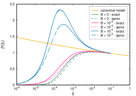
The canonical model plot will be useful not only as a guide to quickly spot the novel features introduced by our model, but also to confirm the fact that, for given a value of , a certain scale can be found where the PPS meets naturally the standard CDM model. This was the spirit in which the value of was adopted, as mentioned above.
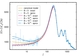
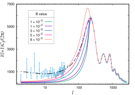
The next step is to analyze the effects of varying the model parameters in the angular power spectrum. To accomplish this, we perform the corresponding modifications in the Code for Anisotropies in the Microwave Background (CAMB) software Lewis et al. (2000). Figure 2 depicts the resulting angular spectrum for different values of .
In order to have a better visualization on the impact our model may have on observational signatures, we show the best–fit CDM prediction for the angular spectrum and the corresponding Planck data444These data points correspond to R3.01 baseline Planck TT, TE, EE+lowE+lensing for multipoles between . Considering lensing effects in our calculations did not show any difference in the result. Therefore, we consider that these data are adequate for making comparisons with our model. together with their error bars (shown in blue). The effect of varying is mainly seen in the low multipoles (). If tends to zero, the CSL spectrum approaches to the one of the original model, and at the same time, it separates from the canonical model at the bottom of the graph. On the contrary, if is increased, the CSL spectrum splits from the canonical model at the top part of the plot corresponding to the lowest multipoles.
The previous analysis indicates that our model has the potential to exhibit different features in the low– range, approaching the CDM angular spectrum from upwards or below, and having the original model as the lower limit. In other words, including the CSL mechanism in the EU model could result not only in a suppression of the temperature anisotropies of the CMB at large angular scales, but also in an excess.
III.1 Further parameter space exploration
From the previous discussion, it is clear that the implementation of the CSL model into the EU scenario could be in good agreement with observational data. However, it is also important to check whether one can, in principle, truly distinguish the predictions between the canonical model and the one proposed in this work. Recall that we have introduced a new parameter , while the combination comes from the original model. Therefore, we are interested in testing the robustness of and in the predicted angular spectrum. In other words, we will vary and enough to see how much our predicted spectrum deviates from the standard one.
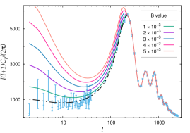
At first glance, one could argue that any well fitted value of would make the model consistent with observations, because any new features introduced in the spectrum could remain masked under the so called cosmic variance. However, exploring a wide range of the parameter space, shows that, even though highest multipoles are unaffected, the first acoustic peak is half missed for increasing values of , see Fig. 3. This suggests that has an upper limit and its value can be constrained with observational data; therefore, the model has predictability.
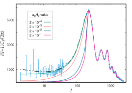
Up to this point, we have worked with the same fixed value of as the one considered in the original model Labraña (2015). Henceforth, it is interesting to explore the possibility to regard the combination as a free parameter. In Fig. 4, we vary along four orders of magnitude. Increasing , implies a strong suppression in the angular power spectrum. This fact indicates that not any value of would make the model consistent with the data. Furthermore, it also indicates that the suppression observed in the original model could be in part explained by a particular combination of the cosmological parameters that has been chosen there.
The final issue we want to address is: given a particular value of that is not compatible with observational data, could it be compensated in some way by varying the parameter introduced by the CSL model? Figure 5 encompasses this question by plotting different values of for a fixed (which has been previously seen not compatible with observational data). Even though the variation of introduces new features and the model predictions might approach to Planck’s data at one end, other sectors of the data are highly missed. Consequently, we can safely state that the parameter cannot compensate the suppression induced by a non-favoured value of .
IV Conclusions
In recent years, the emergent universe (EU) has been studied from different perspectives as a viable cosmological model, which could not only avoid the horizon problem and the initial singularity of the standard approach, but could also account for some anomalies in the observations of the CMB at large angular scales.
Motivated by the recent results of Labraña (2015), where it was shown that a phase of super-inflation prior to that of standard slow-roll inflation (originated in the context of the emergent universe presented in Ellis and Maartens (2004); Ellis et al. (2004)) could explain the power suppression observed in the low multipoles of the CMB, we decided to explore in this work the same emergent universe but within the framework of a particular objective collapse theory, known as Continuous Spontaneous Localization (CSL). The CSL theory has been studied with encouraging results in cosmological applications for several years, as a mechanism to break the original symmetries of the quantum vacuum state of the fields, generating the primordial cosmological perturbations and giving an explanation to the quantum-to-classical transition of such perturbations.
We obtained a prediction for the primordial power spectrum. The computed spectrum can be consistent with CMB observational data, if a particular parameterization for the collapse rate is assumed. The parametrization we considered was also proposed and analyzed in previous works but in the framework of standard inflation. Such a parameterization introduces an extra free parameter , in addition to the parameter of the emergent model studied in Labraña (2015). We also found that the predictions and results of such a work can be recovered, when is chosen.
From the analysis in Sec. III, we have found that implementing the CSL collapse proposal to the emergent universe scenario introduces extra modifications at the lowest multipoles. Specifically, through the CSL-parameter , the angular spectrum in the low multipoles sector, exhibits a suppression or an increment. This is a different feature from what is generically produced in models with a super-inflation phase which only decrease the curve spectrum at large angular scales. On the other hand, in the model proposed in this work, whether there is an excess or suppression, will be determined by a combination of the parameters derived from the original model and the novel one introduced by the collapse rate parameterization. This fact enables our model to introduce some new features in the angular spectrum, particularly in the sector of interest where the so-called low– anomaly is located.
On the other hand, increasing the value of the combination produces a suppression in the lowest multipoles. We have also seen that the variation of the parameter produces opposite (and similiar) effects to . Nevertheless, a suppression of the angular spectrum given by cannot be compensated with an increase of .
One important aspect of our model is that the primordial power spectrum obtained smoothly approaches to the one from the standard model within the observational range of interest. This characteristic constitutes a natural modification of the (temperature) angular spectrum, affecting mainly the lowest multipoles without altering the highest ones (which are already constrained by observations to a high degree of accuracy).
Exploration of the free parameters shows that not any value will make the proposed model consistent with observational data. This suggests that there are good opportunities of effectively constraining the parameter space with the full machinery of statistical analysis based on Monte Carlo–Markov chains for cosmology. Such a scenario gives good predictability to the CSL collapse proposal in the emergent universe model. In fact, we expect that the extra free parameter should take a small value (between and ) but not centered at , which clearly distinguishes our proposal from the one explored in Labraña (2015).
Acknowledgements.
G.R.B. is supported by CONICET (Argentina) and he acknowledges support from grant PIP 112-2017-0100220CO of CONICET (Argentina). G.L. and M.P.P. are supported by CONICET (Argentina), they also acknowledge support from the following project grants: Universidad Nacional de La Plata I+D G175 and PIP 112-2020-0100729CO of CONICET (Argentina). M.P.P. thanks Susana Landau for useful discussions regarding the impact of non–standard cosmological models on CMB angular power spectrum. The authors acknowledge the use of the supercluster MIZTLI of UNAM through project LANCAD-UNAM-DGTIC-132 and thank the people of DGTIC-UNAM for technical and computational support.References
- Ade et al. (2016a) P. A. R. Ade et al. (Planck), Astron. Astrophys. 594, A13 (2016a), eprint 1502.01589.
- Aghanim et al. (2020a) N. Aghanim et al. (Planck), Astron. Astrophys. 641, A1 (2020a), eprint 1807.06205.
- Aghanim et al. (2020b) N. Aghanim et al. (Planck), Astron. Astrophys. 641, A6 (2020b), eprint 1807.06209.
- Scolnic et al. (2018) D. M. Scolnic et al., Astrophys. J. 859, 101 (2018), eprint 1710.00845.
- Alam et al. (2021) S. Alam et al. (eBOSS), Phys. Rev. D 103, 083533 (2021), eprint 2007.08991.
- Starobinsky (1979) A. A. Starobinsky, JETP Lett. 30, 682 (1979).
- Starobinsky (1980) A. A. Starobinsky, Phys. Lett. B91, 99 (1980).
- Guth (1981) A. H. Guth, Phys. Rev. D23, 347 (1981).
- Mukhanov and Chibisov (1981) V. F. Mukhanov and G. V. Chibisov, JETP Lett. 33, 532 (1981), [Pisma Zh. Eksp. Teor. Fiz.33,549(1981)].
- Linde (1982) A. D. Linde, Phys. Lett. B108, 389 (1982).
- Linde (1983) A. D. Linde, Phys. Lett. B 129, 177 (1983).
- Albrecht and Steinhardt (1982) A. Albrecht and P. J. Steinhardt, Phys. Rev. Lett. 48, 1220 (1982).
- Bardeen et al. (1983) J. M. Bardeen, P. J. Steinhardt, and M. S. Turner, Phys. Rev. D28, 679 (1983).
- Brandenberger (1984) R. H. Brandenberger, Nuclear Physics B 245, 328 (1984).
- Hawking (1982) S. W. Hawking, Phys. Lett. 115B, 295 (1982).
- Akrami et al. (2020a) Y. Akrami et al. (Planck), Astron. Astrophys. 641, A10 (2020a), eprint 1807.06211.
- Hinshaw et al. (1996) G. Hinshaw, A. J. Banday, C. L. Bennett, K. M. Gorski, A. Kogut, C. H. Lineweaver, G. F. Smoot, and E. L. Wright, Astrophys. J. 464, L25 (1996), eprint astro-ph/9601061.
- Spergel et al. (2003) D. N. Spergel et al. (WMAP), Astrophys. J. Suppl. 148, 175 (2003), eprint astro-ph/0302209.
- Spergel et al. (2007) D. N. Spergel et al. (WMAP), Astrophys. J. Suppl. 170, 377 (2007), eprint astro-ph/0603449.
- Larson et al. (2011) D. Larson, J. Dunkley, G. Hinshaw, E. Komatsu, M. R. Nolta, C. L. Bennett, B. Gold, M. Halpern, R. S. Hill, N. Jarosik, et al., Astrophys. J. Suppl. 192, 16 (2011), eprint 1001.4635.
- Komatsu et al. (2011) E. Komatsu, K. M. Smith, J. Dunkley, C. L. Bennett, B. Gold, G. Hinshaw, N. Jarosik, D. Larson, M. R. Nolta, L. Page, et al., Astrophys. J. Suppl. 192, 18 (2011), eprint 1001.4538.
- Ade et al. (2014a) P. A. R. Ade et al. (Planck), Astron. Astrophys. 571, A1 (2014a), eprint 1303.5062.
- Ade et al. (2014b) P. A. R. Ade et al. (Planck), Astron. Astrophys. 571, A15 (2014b), eprint 1303.5075.
- Ade et al. (2016b) P. A. R. Ade et al. (Planck), Astron. Astrophys. 594, A16 (2016b), eprint 1506.07135.
- Akrami et al. (2020b) Y. Akrami et al. (Planck), Astron. Astrophys. 641, A7 (2020b), eprint 1906.02552.
- Copi et al. (2007) C. Copi, D. Huterer, D. Schwarz, and G. Starkman, Phys. Rev. D75, 023507 (2007), eprint astro-ph/0605135.
- Copi et al. (2009) C. J. Copi, D. Huterer, D. J. Schwarz, and G. D. Starkman, Mon. Not. Roy. Astron. Soc. 399, 295 (2009), eprint 0808.3767.
- Copi et al. (2010) C. J. Copi, D. Huterer, D. J. Schwarz, and G. D. Starkman, Adv. Astron. 2010, 847541 (2010), eprint 1004.5602.
- Copi et al. (2015) C. J. Copi, D. Huterer, D. J. Schwarz, and G. D. Starkman, Mon. Not. Roy. Astron. Soc. 451, 2978 (2015), eprint 1310.3831.
- Sarkar et al. (2011) D. Sarkar, D. Huterer, C. J. Copi, G. D. Starkman, and D. J. Schwarz, Astropart. Phys. 34, 591 (2011), eprint 1004.3784.
- Efstathiou et al. (2010) G. Efstathiou, Y.-Z. Ma, and D. Hanson, Mon. Not. Roy. Astron. Soc. 407, 2530 (2010), eprint 0911.5399.
- Rakic et al. (2006) A. Rakic, S. Rasanen, and D. J. Schwarz, Mon. Not. Roy. Astron. Soc. 369, L27 (2006), eprint astro-ph/0601445.
- Francis and Peacock (2010) C. L. Francis and J. A. Peacock, Mon. Not. Roy. Astron. Soc. 406, 14 (2010), eprint 0909.2495.
- Schwarz et al. (2016) D. J. Schwarz, C. J. Copi, D. Huterer, and G. D. Starkman, Class. Quant. Grav. 33, 184001 (2016), eprint 1510.07929.
- Perivolaropoulos and Skara (2021) L. Perivolaropoulos and F. Skara (2021), eprint 2105.05208.
- Sokolov (1993) I. Y. Sokolov, Soviet Journal of Experimental and Theoretical Physics Letters 57, 617 (1993).
- Stevens et al. (1993) D. Stevens, D. Scott, and J. Silk, Phys. Rev. Lett. 71, 20 (1993).
- Rocha et al. (2004) G. Rocha, L. Cayón, R. Bowen, A. Canavezes, J. Silk, A. J. Banday, and K. M. Górski, Monthly Notices of the Royal Astronomical Society 351, 769 (2004).
- Campanelli et al. (2007) L. Campanelli, P. Cea, and L. Tedesco, Phys. Rev. D 76, 063007 (2007).
- Bastero-Gil et al. (2003) M. Bastero-Gil, K. Freese, and L. Mersini-Houghton, Phys. Rev. D 68, 123514 (2003), eprint hep-ph/0306289.
- Contaldi et al. (2003) C. R. Contaldi, M. Peloso, L. Kofman, and A. D. Linde, JCAP 07, 002 (2003), eprint astro-ph/0303636.
- Bridle et al. (2003) S. L. Bridle, A. M. Lewis, J. Weller, and G. Efstathiou, Monthly Notices of the Royal Astronomical Society 342, L72 (2003).
- Feng and Zhang (2003) B. Feng and X. Zhang, Phys. Lett. B 570, 145 (2003), eprint astro-ph/0305020.
- Piao et al. (2004) Y.-S. Piao, B. Feng, and X. Zhang, Phys. Rev. D 69, 103520 (2004).
- Boyanovsky et al. (2006) D. Boyanovsky, H. J. de Vega, and N. G. Sanchez, Phys. Rev. D 74, 123007 (2006), eprint astro-ph/0607487.
- Cao et al. (2008) F. J. Cao, H. J. de Vega, and N. G. Sanchez, Phys. Rev. D 78, 083508 (2008), eprint 0809.0623.
- Destri et al. (2008) C. Destri, H. J. de Vega, and N. G. Sanchez, Phys. Rev. D 78, 023013 (2008), eprint 0804.2387.
- Destri et al. (2010) C. Destri, H. J. de Vega, and N. G. Sanchez, Phys. Rev. D 81, 063520 (2010), eprint 0912.2994.
- Handley et al. (2014) W. J. Handley, S. D. Brechet, A. N. Lasenby, and M. P. Hobson, Phys. Rev. D 89, 063505 (2014), eprint 1401.2253.
- Gessey-Jones and Handley (2021) T. Gessey-Jones and W. J. Handley, Phys. Rev. D 104, 063532 (2021), eprint 2104.03016.
- Ramirez and Schwarz (2012) E. Ramirez and D. J. Schwarz, Phys. Rev. D 85, 103516 (2012), eprint 1111.7131.
- Ramirez (2012) E. Ramirez, Phys. Rev. D 85, 103517 (2012).
- Biswas and Mazumdar (2014) T. Biswas and A. Mazumdar, Class. Quant. Grav. 31, 025019 (2014), eprint 1304.3648.
- Liu et al. (2013) Z.-G. Liu, Z.-K. Guo, and Y.-S. Piao, Phys. Rev. D 88, 063539 (2013).
- Liu et al. (2014) Z.-G. Liu, Z.-K. Guo, and Y.-S. Piao, Eur. Phys. J. C 74, 3006 (2014), eprint 1311.1599.
- Ashtekar et al. (2020) A. Ashtekar, B. Gupt, D. Jeong, and V. Sreenath, Phys. Rev. Lett. 125, 051302 (2020), eprint 2001.11689.
- Agullo et al. (2021a) I. Agullo, D. Kranas, and V. Sreenath, Gen. Rel. Grav. 53, 17 (2021a), eprint 2005.01796.
- Agullo et al. (2021b) I. Agullo, D. Kranas, and V. Sreenath, Class. Quant. Grav. 38, 065010 (2021b), eprint 2006.09605.
- Tryon (1973) E. P. Tryon, Nature (London) 246, 396 (1973).
- Vilenkin (1982) A. Vilenkin, Physics Letters B 117, 25 (1982).
- Ellis (1987) G. F. R. Ellis, Astrophys. J. 314, 1 (1987).
- Ellis (1988) G. F. R. Ellis, Classical and Quantum Gravity 5, 891 (1988).
- Ellis et al. (1991) G. F. R. Ellis, D. H. Lyth, and M. B. Mijić, Physics Letters B 271, 52 (1991).
- Linde (1995) A. D. Linde, Phys. Lett. B 351, 99 (1995), eprint hep-th/9503097.
- Linde and Mezhlumian (1995) A. D. Linde and A. Mezhlumian, Phys. Rev. D 52, 6789 (1995), eprint astro-ph/9506017.
- White and Scott (1996) M. J. White and D. Scott, Astrophys. J. 459, 415 (1996), eprint astro-ph/9508157.
- Linde (1998) A. D. Linde, Phys. Rev. D 58, 083514 (1998), eprint gr-qc/9802038.
- Linde (1999) A. D. Linde, Phys. Rev. D 59, 023503 (1999), eprint hep-ph/9807493.
- Ellis et al. (2002) G. F. R. Ellis, W. R. Stoeger, S. J., P. McEwan, and P. Dunsby, Gen. Rel. Grav. 34, 1445 (2002), eprint gr-qc/0109023.
- Linde (2003) A. D. Linde, JCAP 05, 002 (2003), eprint astro-ph/0303245.
- Lasenby and Doran (2005) A. Lasenby and C. Doran, Phys. Rev. D 71, 063502 (2005), eprint astro-ph/0307311.
- Uzan et al. (2003) J.-P. Uzan, U. Kirchner, and G. F. R. Ellis, Mon. Not. Roy. Astron. Soc. 344, L65 (2003), eprint astro-ph/0302597.
- Zhang and Sun (2004) D.-H. Zhang and C.-Y. Sun, Chinese Physics Letters 21, 1865 (2004).
- Ratra (2017) B. Ratra, Phys. Rev. D 96, 103534 (2017), eprint 1707.03439.
- Ooba et al. (2018a) J. Ooba, B. Ratra, and N. Sugiyama, Astrophys. J. 864, 80 (2018a), eprint 1707.03452.
- Räsänen et al. (2015) S. Räsänen, K. Bolejko, and A. Finoguenov, Phys. Rev. Lett. 115, 101301 (2015), eprint 1412.4976.
- Park and Ratra (2019a) C.-G. Park and B. Ratra, Astrophys. J. 882, 158 (2019a), eprint 1801.00213.
- Ryan et al. (2018) J. Ryan, S. Doshi, and B. Ratra, Mon. Not. Roy. Astron. Soc. 480, 759 (2018), eprint 1805.06408.
- Yu et al. (2018) H. Yu, B. Ratra, and F.-Y. Wang, Astrophys. J. 856, 3 (2018), eprint 1711.03437.
- Ooba et al. (2018b) J. Ooba, B. Ratra, and N. Sugiyama, Astrophys. J. 864, 80 (2018b), eprint 1707.03452.
- Park and Ratra (2019b) C.-G. Park and B. Ratra, Astrophys. Space Sci. 364, 134 (2019b), eprint 1809.03598.
- Ryan et al. (2019) J. Ryan, Y. Chen, and B. Ratra, Mon. Not. Roy. Astron. Soc. 488, 3844 (2019), eprint 1902.03196.
- Handley (2021) W. Handley, Phys. Rev. D 103, L041301 (2021), eprint 1908.09139.
- Efstathiou and Gratton (2019) G. Efstathiou and S. Gratton (2019), eprint 1910.00483.
- Riess et al. (2019) A. G. Riess, S. Casertano, W. Yuan, L. M. Macri, and D. Scolnic, Astrophys. J. 876, 85 (2019), eprint 1903.07603.
- Di Valentino et al. (2019) E. Di Valentino, A. Melchiorri, and J. Silk, Nature Astron. 4, 196 (2019), eprint 1911.02087.
- Di Valentino et al. (2021a) E. Di Valentino, A. Melchiorri, and J. Silk, Astrophys. J. Lett. 908, L9 (2021a), eprint 2003.04935.
- Efstathiou and Gratton (2020) G. Efstathiou and S. Gratton, Mon. Not. Roy. Astron. Soc. 496, L91 (2020), eprint 2002.06892.
- Di Valentino et al. (2021b) E. Di Valentino et al., Astropart. Phys. 131, 102607 (2021b), eprint 2008.11286.
- Benisty and Staicova (2021) D. Benisty and D. Staicova, Astron. Astrophys. 647, A38 (2021), eprint 2009.10701.
- Vagnozzi et al. (2021a) S. Vagnozzi, E. Di Valentino, S. Gariazzo, A. Melchiorri, O. Mena, and J. Silk, Phys. Dark Univ. 33, 100851 (2021a), eprint 2010.02230.
- Vagnozzi et al. (2021b) S. Vagnozzi, A. Loeb, and M. Moresco, Astrophys. J. 908, 84 (2021b), eprint 2011.11645.
- Dhawan et al. (2021) S. Dhawan, J. Alsing, and S. Vagnozzi, Mon. Not. Roy. Astron. Soc. 506, L1 (2021), eprint 2104.02485.
- Verde et al. (2019) L. Verde, T. Treu, and A. G. Riess, Nature Astron. 3, 891 (2019), eprint 1907.10625.
- Di Valentino et al. (2021c) E. Di Valentino, O. Mena, S. Pan, L. Visinelli, W. Yang, A. Melchiorri, D. F. Mota, A. G. Riess, and J. Silk, Class. Quant. Grav. 38, 153001 (2021c), eprint 2103.01183.
- Bolejko (2018) K. Bolejko, Phys. Rev. D 97, 103529 (2018), eprint 1712.02967.
- Collett et al. (2019) T. Collett, F. Montanari, and S. Rasanen, Phys. Rev. Lett. 123, 231101 (2019), eprint 1905.09781.
- Clarkson et al. (2007) C. Clarkson, M. Cortes, and B. A. Bassett, JCAP 08, 011 (2007), eprint astro-ph/0702670.
- Hlozek et al. (2008) R. Hlozek, M. Cortes, C. Clarkson, and B. Bassett, Gen. Rel. Grav. 40, 285 (2008), eprint 0801.3847.
- Barenboim et al. (2010) G. Barenboim, E. F. Martínez, O. Mena, and L. Verde, JCAP 03, 008 (2010), eprint 0910.0252.
- Di Valentino et al. (2021d) E. Di Valentino, A. Melchiorri, O. Mena, S. Pan, and W. Yang, Mon. Not. Roy. Astron. Soc. 502, L23 (2021d), eprint 2011.00283.
- Penrose (1965) R. Penrose, Phys. Rev. Lett. 14, 57 (1965).
- Hawking (1965) S. W. Hawking, Phys. Rev. Lett. 15, 689 (1965).
- Hawking and Penrose (1970) S. W. Hawking and R. Penrose, Proceedings of the Royal Society of London Series A 314, 529 (1970).
- Hawking and Ellis (2011) S. W. Hawking and G. F. R. Ellis, The Large Scale Structure of Space-Time, Cambridge Monographs on Mathematical Physics (Cambridge University Press, 2011).
- Wald (1984) R. M. Wald, General Relativity (Chicago Univ. Pr., Chicago, USA, 1984).
- Borde and Vilenkin (1994a) A. Borde and A. Vilenkin, Phys. Rev. Lett. 72, 3305 (1994a), eprint gr-qc/9312022.
- Borde and Vilenkin (1994b) A. Borde and A. Vilenkin, in 8th Nishinomiya-Yukawa Memorial Symposium: Relativistic Cosmology (1994b), eprint gr-qc/9403004.
- Borde (1994) A. Borde, Phys. Rev. D 50, 3692 (1994), eprint gr-qc/9403049.
- Borde and Vilenkin (1996) A. Borde and A. Vilenkin, Int. J. Mod. Phys. D 5, 813 (1996), eprint gr-qc/9612036.
- Borde and Vilenkin (1997) A. Borde and A. Vilenkin, Phys. Rev. D 56, 717 (1997), eprint gr-qc/9702019.
- Guth (2001) A. H. Guth, Annals N. Y. Acad. Sci. 950, 66 (2001), eprint astro-ph/0101507.
- Borde et al. (2003) A. Borde, A. H. Guth, and A. Vilenkin, Phys. Rev. Lett. 90, 151301 (2003), eprint gr-qc/0110012.
- Molina-Paris and Visser (1999) C. Molina-Paris and M. Visser, Phys. Lett. B 455, 90 (1999), eprint gr-qc/9810023.
- Kanekar et al. (2001) N. Kanekar, V. Sahni, and Y. Shtanov, Phys. Rev. D 63, 083520 (2001), eprint astro-ph/0101448.
- Khoury et al. (2001) J. Khoury, B. A. Ovrut, P. J. Steinhardt, and N. Turok, Phys. Rev. D 64, 123522 (2001), eprint hep-th/0103239.
- Steinhardt and Turok (2002) P. J. Steinhardt and N. Turok, Phys. Rev. D 65, 126003 (2002), eprint hep-th/0111098.
- Battefeld et al. (2004) T. J. Battefeld, S. P. Patil, and R. Brandenberger, Phys. Rev. D 70, 066006 (2004), eprint hep-th/0401010.
- Bojowald et al. (2004) M. Bojowald, R. Maartens, and P. Singh, Phys. Rev. D 70, 083517 (2004), eprint hep-th/0407115.
- Biswas et al. (2006) T. Biswas, A. Mazumdar, and W. Siegel, JCAP 03, 009 (2006), eprint hep-th/0508194.
- Peter and Pinto-Neto (2002) P. Peter and N. Pinto-Neto, Phys. Rev. D 66, 063509 (2002), eprint hep-th/0203013.
- Battefeld and Peter (2015) D. Battefeld and P. Peter, Phys. Rept. 571, 1 (2015), eprint 1406.2790.
- Lilley and Peter (2015) M. Lilley and P. Peter, Comptes Rendus Physique 16, 1038 (2015), eprint 1503.06578.
- Brandenberger and Peter (2017) R. Brandenberger and P. Peter, Found. Phys. 47, 797 (2017), eprint 1603.05834.
- Matsui et al. (2019) H. Matsui, F. Takahashi, and T. Terada, Phys. Lett. B 795, 152 (2019), eprint 1904.12312.
- Barrau (2020) A. Barrau, Eur. Phys. J. C 80, 579 (2020), eprint 2005.04693.
- Ellis and Maartens (2004) G. F. R. Ellis and R. Maartens, Class. Quant. Grav. 21, 223 (2004), eprint gr-qc/0211082.
- Einstein (1917) A. Einstein, Sitzungsberichte der Königlich Preußischen Akademie der Wissenschaften (Berlin pp. 142–152 (1917).
- Eddington (1930) A. S. Eddington, Mon. Not. Roy. Astron. Soc. 90, 668 (1930).
- Ellis et al. (2004) G. F. R. Ellis, J. Murugan, and C. G. Tsagas, Class. Quant. Grav. 21, 233 (2004), eprint gr-qc/0307112.
- Mulryne et al. (2005) D. J. Mulryne, R. Tavakol, J. E. Lidsey, and G. F. R. Ellis, Phys. Rev. D 71, 123512 (2005), eprint astro-ph/0502589.
- Gibbons (1987) G. W. Gibbons, Nuclear Physics B 292, 784 (1987).
- Barrow et al. (2003) J. D. Barrow, G. F. R. Ellis, R. Maartens, and C. G. Tsagas, Class. Quant. Grav. 20, L155 (2003), eprint gr-qc/0302094.
- Mukherjee et al. (2005) S. Mukherjee, B. C. Paul, S. D. Maharaj, and A. Beesham (2005), eprint gr-qc/0505103.
- Mukherjee et al. (2006) S. Mukherjee, B. C. Paul, N. K. Dadhich, S. D. Maharaj, and A. Beesham, Class. Quant. Grav. 23, 6927 (2006), eprint gr-qc/0605134.
- Banerjee et al. (2007) A. Banerjee, T. Bandyopadhyay, and S. Chakraborty, Grav. Cosmol. 13, 290 (2007), eprint 0705.3933.
- Boehmer et al. (2007) C. G. Boehmer, L. Hollenstein, and F. S. N. Lobo, Phys. Rev. D 76, 084005 (2007), eprint 0706.1663.
- Parisi et al. (2007) L. Parisi, M. Bruni, R. Maartens, and K. Vandersloot, Class. Quant. Grav. 24, 6243 (2007), eprint 0706.4431.
- del Campo et al. (2007) S. del Campo, R. Herrera, and P. Labrana, JCAP 11, 030 (2007), eprint 0711.1559.
- Debnath (2008) U. Debnath, Class. Quant. Grav. 25, 205019 (2008), eprint 0808.2379.
- Banerjee et al. (2008) A. Banerjee, T. Bandyopadhyay, and S. Chakraborty, Gen. Rel. Grav. 40, 1603 (2008), eprint 0711.4188.
- Beesham et al. (2009) A. Beesham, S. V. Chervon, and S. D. Maharaj, Class. Quant. Grav. 26, 075017 (2009), eprint 0904.0773.
- del Campo et al. (2009) S. del Campo, R. Herrera, and P. Labrana, JCAP 07, 006 (2009), eprint 0905.0614.
- Paul and Ghose (2010) B. C. Paul and S. Ghose, Gen. Rel. Grav. 42, 795 (2010), eprint 0809.4131.
- Paul et al. (2010) B. C. Paul, P. Thakur, and S. Ghose, Mon. Not. Roy. Astron. Soc. 407, 415 (2010), eprint 1004.4256.
- Zhang et al. (2010) K. Zhang, P. Wu, and H. W. Yu, Phys. Lett. B 690, 229 (2010), eprint 1005.4201.
- Paul et al. (2011) B. C. Paul, S. Ghose, and P. Thakur, Mon. Not. R. Astron. Soc. 413, 686 (2011), eprint 1101.1360.
- Chattopadhyay and Debnath (2011) S. Chattopadhyay and U. Debnath, Int. J. Mod. Phys. D 20, 1135 (2011), eprint 1105.1091.
- del Campo et al. (2011) S. del Campo, E. I. Guendelman, A. B. Kaganovich, R. Herrera, and P. Labrana, Phys. Lett. B 699, 211 (2011), eprint 1105.0651.
- del Campo et al. (2010) S. del Campo, E. I. Guendelman, R. Herrera, and P. Labrana, JCAP 06, 026 (2010), eprint 1006.5734.
- Labrana (2012) P. Labrana, Phys. Rev. D 86, 083524 (2012), eprint 1111.5360.
- Cai et al. (2012) Y.-F. Cai, M. Li, and X. Zhang, Phys. Lett. B 718, 248 (2012), eprint 1209.3437.
- Rudra (2012) P. Rudra, Mod. Phys. Lett. A 27, 1250189 (2012), eprint 1211.2047.
- Ghose et al. (2012) S. Ghose, P. Thakur, and B. C. Paul, Mon. Not. R. Astron. Soc. 421, 20 (2012), eprint 1105.3303.
- Liu and Piao (2013) Z.-G. Liu and Y.-S. Piao, Phys. Lett. B 718, 734 (2013), eprint 1207.2568.
- Aguirre and Kehayias (2013) A. Aguirre and J. Kehayias, Phys. Rev. D 88, 103504 (2013), eprint 1306.3232.
- Cai et al. (2014) Y.-F. Cai, Y. Wan, and X. Zhang, Phys. Lett. B 731, 217 (2014), eprint 1312.0740.
- Atazadeh et al. (2014) K. Atazadeh, Y. Heydarzade, and F. Darabi, Phys. Lett. B 732, 223 (2014), eprint 1401.7638.
- Zhang et al. (2014) K. Zhang, P. Wu, and H. Yu, JCAP 01, 048 (2014), eprint 1311.4051.
- Bag et al. (2014) S. Bag, V. Sahni, Y. Shtanov, and S. Unnikrishnan, JCAP 07, 034 (2014), eprint 1403.4243.
- Huang et al. (2015) Q. Huang, P. Wu, and H. Yu, Phys. Rev. D 91, 103502 (2015), eprint 1504.05284.
- Böhmer et al. (2015) C. G. Böhmer, N. Tamanini, and M. Wright, Phys. Rev. D 92, 124067 (2015), eprint 1510.01477.
- Labraña (2015) P. Labraña, Phys. Rev. D 91, 083534 (2015), eprint 1312.6877.
- Khodadi et al. (2016) M. Khodadi, Y. Heydarzade, F. Darabi, and E. N. Saridakis, Phys. Rev. D 93, 124019 (2016), eprint 1512.08674.
- Zhang et al. (2016) K. Zhang, P. Wu, H. Yu, and L.-W. Luo, Physics Letters B 758, 37 (2016).
- Ríos et al. (2016) C. Ríos, P. Labraña, and A. Cid, Journal of Physics: Conference Series 720, 012008 (2016).
- Khodadi et al. (2018) M. Khodadi, K. Nozari, and E. N. Saridakis, Class. Quant. Grav. 35, 015010 (2018), eprint 1612.09254.
- Martineau and Barrau (2018) K. Martineau and A. Barrau, Universe 4, 149 (2018), eprint 1812.05522.
- Labrana and Cossio (2019) P. Labrana and H. Cossio, Eur. Phys. J. C 79, 303 (2019), eprint 1808.09291.
- Brandenberger (2010) R. H. Brandenberger, PoS ICFI2010, 001 (2010), eprint 1103.2271.
- Brandenberger (2020) R. H. Brandenberger, Beyond Standard Inflationary Cosmology (2020), eprint 1809.04926.
- Brandenberger and Vafa (1989) R. Brandenberger and C. Vafa, Nuclear Physics B 316, 391 (1989).
- Nayeri et al. (2006) A. Nayeri, R. H. Brandenberger, and C. Vafa, Phys. Rev. Lett. 97, 021302 (2006), eprint hep-th/0511140.
- Brandenberger (2008) R. H. Brandenberger (2008), eprint 0808.0746.
- Brandenberger (2011) R. H. Brandenberger, Class. Quant. Grav. 28, 204005 (2011), eprint 1105.3247.
- Obied et al. (2018) G. Obied, H. Ooguri, L. Spodyneiko, and C. Vafa (2018), eprint 1806.08362.
- Bedroya and Vafa (2020) A. Bedroya and C. Vafa, JHEP 09, 123 (2020), eprint 1909.11063.
- Garg and Krishnan (2019) S. K. Garg and C. Krishnan, JHEP 11, 075 (2019), eprint 1807.05193.
- Agrawal et al. (2018) P. Agrawal, G. Obied, P. J. Steinhardt, and C. Vafa, Phys. Lett. B 784, 271 (2018), eprint 1806.09718.
- Brandenberger and Martin (2013) R. H. Brandenberger and J. Martin, Class. Quant. Grav. 30, 113001 (2013), eprint 1211.6753.
- Bedroya et al. (2020) A. Bedroya, R. Brandenberger, M. Loverde, and C. Vafa, Phys. Rev. D 101, 103502 (2020), eprint 1909.11106.
- Brandenberger (2021) R. Brandenberger (2021), eprint 2102.09641.
- Wigner (1963) E. P. Wigner, American Journal of Physics 31, 6 (1963).
- Omnes (1994) R. Omnes, The Interpretation of Quantum Mechanics (Princeton University Press, 1994).
- Maudlin (1995) T. Maudlin, Topoi 14, 7 (1995).
- Becker (2018) A. Becker, What is Real? The Unfinished Quest for the Meaning of Quantum Physics (Basic Books, New York, 2018).
- Norsen (2017) T. Norsen, Foundations of Quantum Mechanics (Springer International Publishing AG, 2017).
- Durr and Lazarovici (2020) D. Durr and D. Lazarovici, Understanding Quantum Mechanics (Springer International Publishing AG, 2020).
- Albert (1994) D. Z. Albert, Quantum Mechanics and Experience, (Harvard University Press) (1994).
- Okon (2014) E. Okon, Rev. Mex. Fis. E 60, 130 (2014).
- Bell (1981) J. S. Bell, Quantum Mechanics for cosmologists, Quantum Gravity 2 (eds. Isham, C., Penrose, R. and Sciama, D., Oxford University Press, 1981).
- Perez et al. (2006) A. Perez, H. Sahlmann, and D. Sudarsky, Class. Quant. Grav. 23, 2317 (2006), eprint gr-qc/0508100.
- Sudarsky (2011) D. Sudarsky, Int. J. Mod. Phys. D 20, 509 (2011), eprint 0906.0315.
- Landau et al. (2013) S. Landau, G. León, and D. Sudarsky, Phys. Rev. D 88, 023526 (2013), eprint 1107.3054.
- Hartle (1993) J. B. Hartle, arXiv e-prints gr-qc/9304006 (1993), eprint gr-qc/9304006.
- Berjon et al. (2021) J. Berjon, E. Okon, and D. Sudarsky, Phys. Rev. D 103, 043521 (2021), eprint 2009.09999.
- Bengochea (2020) G. R. Bengochea, Rev. Mex. Fis. E 17, 263 (2020), eprint 2007.03428.
- Bohm (1952) D. Bohm, Phys. Rev. 85, 166 (1952).
- Valentini (2010) A. Valentini, Phys. Rev. D 82, 063513 (2010), eprint 0805.0163.
- Pinto-Neto et al. (2012) N. Pinto-Neto, G. Santos, and W. Struyve, Phys. Rev. D 85, 083506 (2012), eprint 1110.1339.
- Goldstein et al. (2015) S. Goldstein, W. Struyve, and R. Tumulka, arXiv e-prints arXiv:1508.01017 (2015), eprint 1508.01017.
- Pinto-Neto and Struyve (2018) N. Pinto-Neto and W. Struyve, arXiv e-prints arXiv:1801.03353 (2018), eprint 1801.03353.
- Vitenti et al. (2019) S. D. P. Vitenti, P. Peter, and A. Valentini, Phys. Rev. D 100, 043506 (2019), eprint 1901.08885.
- Kiefer and Polarski (2009) C. Kiefer and D. Polarski, Adv. Sci. Lett. 2, 164 (2009), eprint 0810.0087.
- Halliwell (1989) J. J. Halliwell, Phys. Rev. D39, 2912 (1989).
- Kiefer (2000) C. Kiefer, Nucl. Phys. Proc. Suppl. 88, 255 (2000), eprint astro-ph/0006252.
- Polarski and Starobinsky (1996) D. Polarski and A. A. Starobinsky, Class. Quant. Grav. 13, 377 (1996), eprint gr-qc/9504030.
- Okon and Sudarsky (2016) E. Okon and D. Sudarsky, Found. Phys. 46, 852 (2016), eprint 1512.05298.
- Adler (2003) S. L. Adler, Studies in History and Philosophy of Modern Physics 34, 135 (2003), eprint quant-ph/0112095.
- Schlosshauer (2004) M. Schlosshauer, Rev. Mod. Phys. 76, 1267 (2004), eprint quant-ph/0312059.
- Everett (1957) H. Everett, Rev. Mod. Phys. 29, 454 (1957).
- Mukhanov (2005) V. Mukhanov, Physical Foundations of Cosmology (New York: Cambridge University Press, 2005).
- Kent (1990) A. Kent, International Journal of Modern Physics A 5, 1745 (1990), eprint gr-qc/9703089.
- Stapp (2002) H. P. Stapp, Canadian Journal of Physics 80, 1043 (2002), eprint quant-ph/0110148.
- Pearle (1976) P. Pearle, Phys. Rev. D 13, 857 (1976).
- Ghirardi et al. (1986) G. Ghirardi, A. Rimini, and T. Weber, Phys.Rev. D34, 470 (1986).
- Pearle (1989) P. M. Pearle, Phys.Rev. A39, 2277 (1989).
- Diosi (1987) L. Diosi, Phys.Lett. A120, 377 (1987).
- Diosi (1989) L. Diosi, Phys.Rev. A40, 1165 (1989).
- Penrose (1996) R. Penrose, Gen.Rel.Grav. 28, 581 (1996).
- Okon and Sudarsky (2014) E. Okon and D. Sudarsky, Found. Phys. 44, 114 (2014), eprint 1309.1730.
- Bassi and Ghirardi (2003) A. Bassi and G. Ghirardi, Phys. Rept. 379, 257 (2003), eprint quant-ph/0302164.
- Bassi et al. (2013) A. Bassi, K. Lochan, S. Satin, T. P. Singh, and H. Ulbricht, Reviews of Modern Physics 85, 471 (2013), eprint 1204.4325.
- Leon and Sudarsky (2010) G. Leon and D. Sudarsky, Class. Quant. Grav. 27, 225017 (2010), eprint 1003.5950.
- Diez-Tejedor and Sudarsky (2012) A. Diez-Tejedor and D. Sudarsky, JCAP 07, 045 (2012), eprint 1108.4928.
- Diez-Tejedor et al. (2012) A. Diez-Tejedor, G. León, and D. Sudarsky, General Relativity and Gravitation 44, 2965 (2012), eprint 1106.1176.
- Cañate et al. (2013) P. Cañate, P. Pearle, and D. Sudarsky, Phys.Rev. D 87, 104024 (2013), eprint 1211.3463.
- Bengochea et al. (2015) G. R. Bengochea, P. Cañate, and D. Sudarsky, Phys. Lett. B743, 484 (2015), eprint 1410.4212.
- León and Sudarsky (2015) G. León and D. Sudarsky, JCAP 06, 020 (2015), eprint 1503.01417.
- Leon and Bengochea (2016) G. Leon and G. R. Bengochea, Eur. Phys. J. C76, 29 (2016), eprint 1502.04907.
- León (2017) G. León, European Physical Journal C 77, 705 (2017), eprint 1705.03958.
- Landau et al. (2012) S. J. Landau, C. G. Scóccola, and D. Sudarsky, Physical Review D 85, 123001 (2012), eprint 1112.1830.
- Benetti et al. (2016) M. Benetti, S. J. Landau, and J. S. Alcaniz, JCAP 12, 035 (2016), eprint 1610.03091.
- Bengochea and León (2017) G. R. Bengochea and G. León, Phys. Lett. B 774, 338 (2017), eprint 1708.07527.
- Cañate et al. (2018) P. Cañate, E. Ramirez, and D. Sudarsky, JCAP 08, 043 (2018), eprint 1802.02238.
- Juárez-Aubry et al. (2018) B. A. Juárez-Aubry, B. S. Kay, and D. Sudarsky, Phys. Rev. D 97, 025010 (2018), eprint 1708.09371.
- Piccirilli et al. (2019) M. P. Piccirilli, G. León, S. J. Landau, M. Benetti, and D. Sudarsky, International Journal of Modern Physics D 28, 1950041 (2019), eprint 1709.06237.
- León et al. (2015) G. León, L. Kraiselburd, and S. J. Landau, Phys. Rev. D 92, 083516 (2015), eprint 1509.08399.
- Mariani et al. (2016) M. Mariani, G. R. Bengochea, and G. León, Physics Letters B 752, 344 (2016), eprint 1412.6471.
- León et al. (2017) G. León, A. Majhi, E. Okon, and D. Sudarsky, Phys. Rev. D 96, 101301 (2017), eprint 1607.03523.
- León et al. (2018) G. León, A. Majhi, E. Okon, and D. Sudarsky, Phys. Rev. D 98, 023512 (2018), eprint 1712.02435.
- León et al. (2016) G. León, G. R. Bengochea, and S. J. Landau, European Physical Journal C 76, 407 (2016), eprint 1605.03632.
- Josset et al. (2017) T. Josset, A. Perez, and D. Sudarsky, Phys. Rev. Lett. 118, 021102 (2017), eprint 1604.04183.
- Leon and Piccirilli (2020) G. Leon and M. P. Piccirilli, Phys. Rev. D 102, 043515 (2020), eprint 2006.03092.
- Martin et al. (2012) J. Martin, V. Vennin, and P. Peter, Phys. Rev. D 86, 103524 (2012), eprint 1207.2086.
- Das et al. (2013) S. Das, K. Lochan, S. Sahu, and T. P. Singh, Phys. Rev. D 88, 085020 (2013), eprint 1304.5094.
- Markkanen et al. (2015) T. Markkanen, S. Rasanen, and P. Wahlman, Phys. Rev. D 91, 084064 (2015), eprint 1407.4691.
- Alexander et al. (2016) S. Alexander, D. Jyoti, and J. Magueijo, Phys. Rev. D 94, 043502 (2016), eprint 1602.01216.
- Drossel and Ellis (2018) B. Drossel and G. Ellis, New Journal of Physics 20, 113025 (2018), eprint 1807.08171.
- Martin and Vennin (2020) J. Martin and V. Vennin, Phys. Rev. Lett. 124, 080402 (2020), eprint 1906.04405.
- Bengochea et al. (2020a) G. R. Bengochea, G. Leon, P. Pearle, and D. Sudarsky (2020a), eprint 2006.05313.
- Bengochea et al. (2020b) G. R. Bengochea, G. León, P. Pearle, and D. Sudarsky, Eur. Phys. J. C 80, 1021 (2020b), eprint 2008.05285.
- Martin and Vennin (2021a) J. Martin and V. Vennin, Eur. Phys. J. C 81, 64 (2021a), eprint 2010.04067.
- Gundhi et al. (2021) A. Gundhi, J. L. Gaona-Reyes, M. Carlesso, and A. Bassi, Phys. Rev. Lett. 127, 091302 (2021), eprint 2102.07688.
- Martin and Vennin (2021b) J. Martin and V. Vennin, Eur. Phys. J. C 81, 516 (2021b), eprint 2103.01697.
- León and Bengochea (2021) G. León and G. R. Bengochea, Eur. Phys. J. C 81, 1055 (2021), eprint 2107.05470.
- Juárez-Aubry et al. (2020) B. A. Juárez-Aubry, T. Miramontes, and D. Sudarsky, J. Math. Phys. 61, 032301 (2020), eprint 1907.09960.
- Eppley and Hannah (1977) K. Eppley and E. Hannah, Foundations of Physics 7, 51 (1977).
- Page and Geilker (1981) D. N. Page and C. D. Geilker, Phys. Rev. Lett. 47, 979 (1981).
- Mattingly (2005) J. Mattingly, Is Quantum Gravity Necessary? (2005), vol. 11, pp. 327–338.
- Mattingly (2006) J. Mattingly, Phys. Rev. D73, 064025 (2006), eprint gr-qc/0601127.
- Kent (2018) A. Kent, Class. Quant. Grav. 35, 245008 (2018), eprint 1807.08708.
- Tilloy and Diósi (2016) A. Tilloy and L. Diósi, Phys. Rev. D93, 024026 (2016), eprint 1509.08705.
- Carlip (2008) S. Carlip, Class. Quant. Grav. 25, 154010 (2008), eprint 0803.3456.
- Albers et al. (2008) M. Albers, C. Kiefer, and M. Reginatto, Phys. Rev. D78, 064051 (2008), eprint 0802.1978.
- Ford (2005) L. H. Ford, 100 Years Of Relativity : space-time structure: Einstein and beyond pp. 293–310 (2005), eprint gr-qc/0504096.
- Ford (2005) L. H. Ford, Spacetime in Semiclassical Gravity (2005), pp. 293–310.
- Piscicchia et al. (2017) K. Piscicchia, A. Bassi, C. Curceanu, R. Grande, S. Donadi, B. Hiesmayr, and A. Pichler, Entropy 19, 319 (2017), eprint 1710.01973.
- Lewis et al. (2000) A. Lewis, A. Challinor, and A. Lasenby, Astrophys. J. 538, 473 (2000), eprint astro-ph/9911177.