What’s inside a hairy black hole in massive gravity?

Abstract

In the context of massive gravity theories, we study holographic flows driven by a relevant scalar operator and interpolating between a UV 3-dimensional CFT and a trans-IR Kasner universe. For a large class of scalar potentials, the Cauchy horizon never forms in presence of a non-trivial scalar hair, although, in absence of it, the black hole solution has an inner horizon due to the finite graviton mass. We show that the instability of the Cauchy horizon triggered by the scalar field is associated to a rapid collapse of the Einstein-Rosen bridge. The corresponding flows run smoothly through the event horizon and at late times end in a spacelike singularity at which the asymptotic geometry takes a general Kasner form dominated by the scalar hair kinetic term. Interestingly, we discover deviations from the simple Kasner universe whenever the potential terms become larger than the kinetic one. Finally, we study the effects of the scalar deformation and the graviton mass on the Kasner singularity exponents and show the relationship between the Kasner exponents and the entanglement and butterfly velocities probing the black hole dynamics. Differently from the holographic superconductor case, we can prove explicitly that Josephson oscillations in the interior of the BH are absent.

1 Introduction

Understanding the interior of a black hole is an intriguing and fundamental problem from both theoretical and experimental perspectives. Due to the highly non-linear nature of the Einstein’s equations, it is typically difficult to obtain black hole solutions analytically. As a matter of fact, the structure and dynamics of the black hole interior, in particular, the region near the black hole singularity where the spacetime curvature becomes infinite, are still elusive concepts. Nevertheless, some analytical black hole solutions were found in the past. The first case is the neutral Schwarzschild black hole whose geometry displays an event horizon and a spacelike singularity within it Schwarzschild:1916uq . Other examples include Reissner- Nordstrom (RN) https://doi.org/10.1002/andp.19163550905 ; 1918KNAB…20.1238N and Kerr black holes  PhysRevLett.11.237 , corresponding to the cases with non-trivial electric charge and angular momentum, respectively. Both have an additional inner Cauchy horizon that represents a breakdown of predictability in general relativity and present a timelike singularity, appearing to violate the strong cosmic censorship (SCC) conjecture  1969NCimR…1..252P . More recently, in the framework of General Relativity, it has been shown that there is no Cauchy horizon for some kind of black holes with scalar hairs and symmetric horizons Hartnoll:2020rwq ; Cai:2020wrp ; Hartnoll:2020fhc ; Devecioglu:2021xug ; An:2021plu ; Grandi:2021ajl . Under quite general conditions, the authors of Yang:2021civ showed that the number of horizons is highly constrained by classical matter.

On the other side, Holography Maldacena:1997re provides some important and promising probes of the black hole interior, such as correlation functions Fidkowski:2003nf ; Festuccia:2005pi , entanglement entropy Hartman:2013qma and complexity Stanford:2014jda ; Brown:2015bva . Following this line of investigation, recently the authors of Frenkel:2020ysx considered a deformation of a thermal CFT state by a relevant scalar operator, which in the bulk yields a deformation of the Schwarzschild singularity, at late interior times, into a more general Kasner form.  This provides a first step beyond the non-generic and classically unstable black hole interiors which have been the main focus of previous holographic literature. At this point, it is imperative to extend such study to more general cases and to uncover possible novel features. One interesting case is that of massive gravity Hinterbichler:2011tt ; Rubakov:2008nh ; Dubovsky:2004sg in which the standard general relativity framework is modified by endowing the graviton with a nonzero mass. From the holographic perspective, massive gravity and the consequent (partial or not) breaking of diffeomorphisms invariance, realizes in a simple and effective way (in fact retaining the homogeneity of the background geometry) the breaking of translational invariance in the dual field theory Vegh:2013sk . In general, it is very helpful to write down the massive gravity theory in the so-called Stueckelberg form  Baggioli:2014roa ; Alberte:2015isw where it appears as a simple set of shift-invariant massless scalar coupled to canonical massless gravity. The usages of this class of models in the Holographic community are very vast, specially in view of the applications to strongly coupled matter Alberte:2016xja ; Alberte:2017cch ; Alberte:2017oqx ; Baggioli:2020edn . We refer the Reader to Baggioli:2021xuv for a complete and exhaustive review on the topic.

In the present work, in the context of the holographic massive gravity framework of  Baggioli:2014roa ; Alberte:2015isw , we study holographic renormalization group flows induced by a neutral scalar field $\phi$ and interpolating between a 3-dimensional UV CFT and a singular Kasner-like universe in the trans-IR . In contrast to the previous cases Frenkel:2020ysx ; Wang:2020nkd where the hairless background is given by the Schwarzschild solution lacking the Cauchy horizon, in the massive gravity case the black hole solution in the absence of the scalar hair $\phi$ can have an inner horizon due to the mass of graviton, which in some sense acts as a charge for the black hole. We consider a relevant deformation of the dual CFT thermal state leading to a holographic renormalization group (RG) flow at finite temperature. Although in our framework, in absence of scalar hair, the black hole presents an inner Cauchy due to the finite graviton mass, the deformation induced by a neutral scalar operator generically removes this Cauchy horizon such that the deformed black hole with non-trivial scalar hair approaches a spacelike singularity at late interior time. The instability of the Cauchy horizon triggered by the scalar field leads to a rapid collapse of the Einstein-Rosen bridge at the would-be Cauchy horizon. The asymptotic geometry near the spacelike singularity is shown to take a general Kasner form whenever the kinetic term of the scalar field $\phi$ dominates. On the contrary, when the potential terms for $\phi$ become important, we find novel and interesting deviations from the standard Kasner universe. Additionally, we prove analytically that, contrarily to the holographic superconductor case of Hartnoll:2020fhc , no Josephson oscillations are present in our case. Our findings suggest that such oscillations do not appear in the absence of background charge and a non-trivial bulk gauge field.

Given these general facts, we also present a more detailed analysis of the black hole interior geometry in function of the various parameters of the model such as the graviton mass. Finally, we probe the aforementioned black hole interior by computing the entanglement velocity and butterfly velocity for the deformed black holes displaying a Kasner singularity at late times.

The rest of the paper is organized as follows. In Section 2, we introduce the gravitational model used in this work, a general four dimensional massive gravity theory coupled to a neutral scalar field $\phi$. We present analytic black hole solutions without the scalar hair and prove the absence of a Cauchy-horizon for the hairy black holes. In Section 3 we discuss the collapse of the Einstein-Rosen bridge associated with the instability of the inner Cauchy horizon triggered by the scalar field. In Section 4, we construct the holographic flows from the AdS boundary to the Kasner singularity sourced by the scalar field. In Section 5, we prove analytically the absence of Josephson oscillations in our holographic model. The violation of the Kasner form near the spacelike singularity is also discussed. The probes of the Kasner exponent are considered in Section 6. We conclude with a brief discussion and some remarks for the future in Section 7.

2 Holographic setup

We consider the following 4-dimensional bulk action

$$S=\frac{1}{16\pi G}\int dx^{4}\sqrt{-g}\Big{[}(R-2\Lambda)-K(X)-\partial^{\mu}\phi\partial_{\mu}\phi-V(\phi^{2})\Big{]}\,,$$ (1)

where $G$ is the Newton constant, $R$ the Ricci scalar, $\Lambda$ the cosmological constant and $\phi$ a neutral bulk scalar field whose potential is denoted as $V$. Additionally, we have introduced a set of shift-invariant massless scalar fields $\Phi^{I}(I=x,y)$ via their kinetic term $X\equiv\frac{1}{2}\sum_{I=1}^{2}\partial_{\mu}\Phi^{I}\partial^{\mu}\Phi^{I}$. Here $K$ is a generic scalar function Baggioli:2014roa ; Baggioli:2016rdj which is sometimes labelled as K-essence Baggioli:2021ejg . The bulk solution for the axion fields $\Phi^{I}$ is taken to be

$$\Phi^{I}=\alpha\,x^{I},$$ (2)

with $\alpha$ a constant. In this sense, these scalars break translational invariance and they provide a mass for the graviton Hinterbichler:2011tt ; Rubakov:2008nh ; Dubovsky:2004sg ; they are indeed nothing else that the Stueckelberg fields which do restore diffeomorphism invariance in our massive gravity theory. In addition, the rest of the solution is parametrized as

$$ds^{2}=\frac{1}{r^{2}}\left(-f(r)e^{-\chi(r)}dt^{2}+\frac{dr^{2}}{f(r)}+dx^{2}+dy^{2}\right),\quad\phi=\phi(r)\,,$$ (3)

where, in our coordinate system, the AdS boundary is at $r=0$ and the black hole singularity locates at $r\to\infty$. Moreover, at the event horizon $r_{+}$, the blackening function $f(r_{+})$ vanishes. From (1), the independent equations of motion read

$$r^{4}e^{\frac{\chi}{2}}\left(\frac{e^{-\frac{\chi}{2}}f\phi^{\prime}}{r^{2}}\right)^{\prime} = \frac{\mathrm{d}{V}}{\mathrm{d}{\phi^{2}}}\phi\,,$$ (4)

$$\chi^{\prime} = r(\phi^{\prime})^{2}\,,$$ (5)

$$4e^{\frac{\chi}{2}}r^{4}\left(\frac{e^{-\frac{\chi}{2}}}{r^{3}}f\right)^{\prime} = 2V(\phi^{2})+2K(\alpha^{2}r^{2})-12\,,$$ (6)

with a prime denoting the derivative with respect to $r$. We have also chosen the cosmological constant $\Lambda=-3/L^{2}$ with the AdS radius $L$ set to one. In general, these coupled differential equations do not allow analytical solutions, thus one has to solve them numerically.

Depending on the choice of the potential $K(X)$, the model in Eq. (1) corresponds to different boundary field theories. In particular, the shape of the potential and its behaviour near the AdS boundary at $r=0$ determines whether translational invariance is broken explicitly or spontaneously in the dual field theory picture Baggioli:2021xuv ; Ammon:2019wci . In the present work, we are interested in the following two cases:

• Type I: $K(X)=X$, which corresponds to the well-known linear axion model  Andrade:2013gsa .

• Type II: $K(X)=a_{1}\sqrt{X}+a_{2}X$ with $a_{1}$ and $a_{2}$ two constants. This form of potential corresponds to the non-linear dRGT massive gravity model Vegh:2013sk as proven in Alberte:2015isw .

We stress that $K^{\prime}(X)>0$ to avoid ghost instability Alberte_2018 . Both type I and type II corresponds to the explicit breaking of translations in the dual field theory and their physics is that described by momentum dissipation.

To continue, near the AdS boundary $r\to 0$, the asymptotic expansion for the various fields $\{\phi,\chi,f\}$ is, respectively, given as follows:

$$\phi = \phi_{0}\,r+\left\langle O\right\rangle r^{2}+...\,,$$ (7)

$$\chi = \frac{\phi_{0}^{2}}{2}\,r^{2}+\frac{4\phi_{0}\left\langle O\right\rangle}{3}r^{3}+...\,,$$ (8)

$$f = \begin{cases}1-\frac{\alpha^{2}}{2}r^{2}+\phi_{0}^{2}r^{2}-\left\langle T_{tt}\right\rangle r^{3}+...\,,\hskip 59.75078pt\text{for type I}\\ 1-\frac{\alpha\,a_{1}}{4}r-\frac{\alpha^{2}\,a_{2}}{2}r^{2}+\phi_{0}^{2}r^{2}-\left\langle T_{tt}\right\rangle r^{3}+...\,,\hskip 14.22636pt\text{for type II}\end{cases}$$ (9)

where we have considered the scalar potential $V(\phi^{2})=m^{2}\phi^{2}$ with $m^{2}=-2$, and have taken the normalization of the time coordinate at the boundary such that $\chi(r=0)=0$. Here, $\phi_{0}$ is the source of the scalar operator of the boundary field theory and $\left\langle O\right\rangle$ the corresponding expectation value.  $\left\langle T_{tt}\right\rangle$ is the energy density of the thermal state in the boundary field theory, and the corresponding temperature reads

$$T=-\frac{f^{\prime}e^{-\frac{\chi}{2}}}{4\pi}\Big{|}_{r=r_{+}}\,.$$ (10)

After imposing regularity at the horizon, $r=r_{+}$, one can write down $\left\langle O\right\rangle$ and $\left\langle T_{tt}\right\rangle$ in terms of $T$, $\phi_{0}$ and $\alpha$. Nevertheless, our system enjoys the following scaling symmetry

$$r\rightarrow r/\lambda,\quad(\phi_{0},T,\alpha)\rightarrow\lambda(\phi_{0},T,\alpha),\quad\left\langle O\right\rangle\rightarrow\lambda^{2}\left\langle O\right\rangle,\quad\left\langle T_{tt}\right\rangle\rightarrow\lambda^{3}\left\langle T_{tt}\right\rangle\,,$$ (11)

with $\lambda$ a constant parameter. Therefore, without loss of generality, we shall work with dimensionless quantities in units of $T$. All in all, the final full solution is then parametrized solely by the dimensionless combinations $\phi_{0}/T$ and $\alpha/T$. For convenience, we fix $r_{+}=1$ in all the manuscript.

2.1 Black holes with no scalar hair

The black hole solutions of (4)-(6) in the absence of the scalar $\phi$ can be obtained analytically (see Baggioli:2014roa for the general solution). It is clear that the only non-trivial equation is (6) when $\phi=0$.

For the linear axion model (type I), from (6), we obtain

$$f(r)=1-\frac{\alpha^{2}r^{2}}{2}+\frac{r^{3}}{r_{+}}\left(\frac{\alpha^{2}}{2}-\frac{1}{r_{+}^{2}}\right)\,.$$ (12)

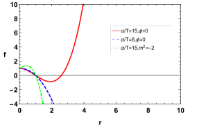
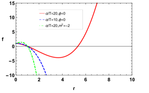
Figure 1: The blackening factor $f(r)$ as a function of $r$ from the boundary $r=0$ to near the black hole singularity $r=\infty$. The left panel refers to the type I linear axion case with $K=X$, while the right panel to the dRGT type II scenario $K=a_{1}\sqrt{X}+a_{2}X$ with $a_{1}=0.1$ and $a_{2}=0.3$.

The interior of the black hole depends on the choice of the parameter $\alpha$ which determines the size of the graviton mass and the rate of translations breaking in the dual field theory Davison:2013jba . When $0\leq\alpha<\sqrt{2}/r_{+}$, the black hole has no inner Cauchy horizon inside the event horizon $r_{+}$, and the interior geometry will end at a spacelike singularity. For other cases, there is typically an inner horizon, for which the singularity is timelike. See the left panel of Fig. 1 for an illustration.

For the dRGT case with $K=a_{1}\sqrt{X}+a_{2}X$ (type II), the black brane solution takes the form

$$f(r)=1-\left(\frac{r}{r_{+}}\right)^{3}-\frac{a_{1}\,\alpha}{4}\left(r-r_{+}\left(\frac{r}{r_{+}}\right)^{3}\right)-\frac{a_{2}\,\alpha^{2}}{2}\left(r^{2}-r_{+}^{2}\left(\frac{r}{r_{+}}\right)^{3}\right)\,.$$ (13)

In this case, the black hole has both an event horizon and an inner horizon, except when

$$a_{1}<\,\frac{4}{r_{+}\,\alpha}\,\quad\text{and}\,\quad a_{2}\,<\,\frac{4-a_{1}\,r_{+}\,\alpha}{2\,r_{+}^{2}\,\alpha^{2}}$$ (14)

for which the inner horizon is absent (see the right panel of Fig. 1).

2.2 Proof of no inner-horizon

Following Ref. Hartnoll:2020rwq , let’s prove the absence of an inner-horizon in the model defined in Eq. (1). Suppose the existence of an inner horizon at $r_{\mathcal{I}}>r_{+}$, for which one has $f(r_{\mathcal{I}})=f(r_{+})=0$. From Eq. (4), we obtain

$$\int_{r_{+}}^{r_{\mathcal{I}}}\left(\frac{fe^{-\frac{\chi}{2}}\phi\phi^{\prime}}{r^{2}}\right)^{\prime}dr=\int_{r_{+}}^{r_{\mathcal{I}}}e^{-\frac{\chi}{2}}{r^{-4}}\left(\frac{\mathrm{d}{V}}{\mathrm{d}{\phi^{2}}}\phi^{2}+r^{2}f(\phi^{\prime})^{2}\right)dr\,.$$ (15)

Clearly, the left hand side yields

$$\int_{r_{+}}^{r_{\mathcal{I}}}\left(\frac{fe^{-\frac{\chi}{2}}\phi\phi^{\prime}}{r^{2}}\right)^{\prime}dr=\frac{fe^{-\frac{\chi}{2}}\phi\phi^{\prime}}{r^{2}}\Big{|}_{r_{\mathcal{I}}}^{r_{+}}=0\,,$$ (16)

where we have used the fact that $f(r_{\mathcal{I}})=f(r_{+})=0$. On the other hand, since $f(r)$ is negative between the two horizons, when we take $\frac{\mathrm{d}{V}}{\mathrm{d}{\phi^{2}}}<0$ for every value of $\phi$, the integrand in the right hand is negative. Therefore, the only way there can be two horizons is for $\phi=0$. The presence of the scalar hair, $\phi\neq 0$, necessarily removes the inner horizon. For example, for the free scalar case with $V=m^{2}\phi^{2}$, the inner horizon will not appear when $m^{2}<0$ corresponding to relevant operators in the boundary theory. Notice that the cases of irrelevant operators $m^{2}>0$ or any other possible potential with $\frac{\mathrm{d}{V}}{\mathrm{d}{\phi^{2}}}$ positive evade this proof and therefore the inner horizon could appear again.

3 Collapse of the Einstein-Rosen bridge

As we have proved in the last section, the black hole with non-trivial scalar hair has no inner horizon, and the black hole interior ends at a spacelike singularity at $r\to\infty$. Following the spirit of Ref. Hartnoll:2020rwq , we do expect to see a crossover around $r_{\mathcal{I}}$, i.e. the position of the would-be inner horizon. In particular, in absence of scalar hair, $\phi=0$, there is typically an inner horizon at $r=r_{\mathcal{I}}$ for the black hole solutions (12) and (13) in the massive gravity theory considered. However, no matter how small the scalar hair is, it has strong non-linear effect closed to the would-be inner Cauchy horizon of  (12) and (13), triggering an instability of the latter.

This crossover can be obtained analytically when the scalar field is small. Note however that the spacetime dynamics is highly nonlinear in the small scalar field limit. This fact is associated with a collapse of the Einstein-Rosen bridge between the two asymptotic boundaries . The main idea of Ref. Hartnoll:2020rwq is that for vanishing small scalar field the instability becomes so fast that one can essentially keep the $r$ coordinate fixed. Let’s set $r=r_{\mathcal{I}}+\delta r$, so that $f$, $\chi$ and $\phi$ are now functions of $\delta r$, while any explicit factors of $r$ in the equations of motion (4)- (6) are set to $r_{\mathcal{I}}$.

For simplicity, we consider $V(\phi^{2})=m^{2}\phi^{2}$. Around the location of the would-be inner horizon, $r=r_{\mathcal{I}}$, the mass of the scalar field can be neglected in (4) and (6) Hartnoll:2020rwq . By using this approximation, one obtains

$$\left(e^{-\chi/2}f\phi^{\prime}\right)^{\prime}=0,\hskip 14.22636pt4r_{\mathcal{I}}f^{\prime}=2r_{\mathcal{I}}^{2}f(\phi^{\prime})^{2}+2K(\alpha^{2}r_{\mathcal{I}}^{2})-12,\hskip 14.22636pt\chi^{\prime}=r_{\mathcal{I}}(\phi^{\prime})^{2}\,.$$ (17)

Integrating the first equation and writing $\phi^{\prime}=-c_{1}(K(z_{\mathcal{I}}^{2}\alpha^{2})-6)^{1/2}e^{\chi/2}/f$ with $c_{1}$ an unspecified constant, one finds the general solution to above equations. In particular, the metric component $g_{tt}=-fe^{-\chi}/r_{\mathcal{I}}^{2}$ is found to obey Hartnoll:2020rwq

$$c_{1}^{2}\log(g_{tt})+g_{tt}=-\frac{r_{\mathcal{I}}}{2}\,c_{2}^{2}(\delta r+c_{3})\,,$$ (18)

with $c_{2}$ and $c_{3}$ two different constants. Making use of Eq. (17) and the above solution, one obtains

$$\phi=-\frac{2c_{1}}{r_{\mathcal{I}}c_{2}}\log\left(c_{4}\,g_{tt}\right)\,,\qquad e^{-\chi}=\frac{2z_{\mathcal{I}}^{4}}{c_{1}^{2}(K(r_{\mathcal{I}}^{2}\alpha^{2})-6)}(\phi^{\prime})^{2}g_{tt}^{2}\,.$$ (19)

Clearly, the scalar field shows a logarithmic growth as the metric component $g_{tt}$ becomes small close to the would-be inner horizon.

As pointed out in Hartnoll:2020rwq , the value of $c_{2}/c_{1}$ will be large when the boundary source for the scalar $\phi$ is small. We check numerically in Fig. 2 that indeed the ratio $c_{2}/c_{1}$ scales as $\sim T/\phi_{(0)}$ as the source $\phi_{(0)}/T\to 0$. Therefore, the term $(c_{2}/c_{1})^{2}\delta r$ in (18) can become very large, which in turn allows the metric component $g_{tt}$ to undergo a suddenly change in the vicinity of $r_{\mathcal{I}}$.

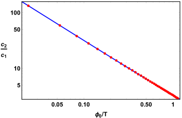
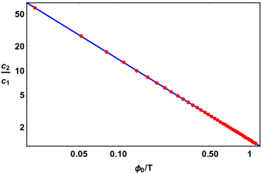
Figure 2: The ratio $c_{2}/c_{1}$ as a function of the dimensionless scalar source $\phi_{0}/T$. The blue lines show the theoretical prediction $c_{2}/c_{1}=a+bT/\phi_{0}$. Left panel: Type I model $K=X$ with $\alpha/T=19.8$. Right panel: Type II case with $K=0.1\sqrt{X}+0.3X$. We have fixed $\alpha/T=24.95$.

Near the would-be inner horizon, for $r<r_{\mathcal{I}}$ (or $\delta r<0$), $g_{tt}\propto\frac{r_{\mathcal{I}}c_{2}^{2}}{2}\delta r$ vanishes linearly towards $r_{\mathcal{I}}$, while for $r>r_{\mathcal{I}}$ (or $\delta r>0$) one observes a rapid collapse of $g_{tt}$ to an exponentially small value, i.e. $g_{tt}\propto e^{-(c_{2}/\sqrt{2}c_{1})^{2}r_{\mathcal{I}}\delta r}$. Note that this collapse occurs over a coordinate range $\Delta r=(c_{1}/c_{2})^{2}$ as illustrated in Hartnoll:2020fhc . This behavior is illustrated in Fig. 3 for a small value of the scalar source $\frac{\phi_{0}}{T}=0.5$ in both Type I and II cases. In addition, the scalar field derivative changes from $\phi^{\prime}=c_{1}/(c_{2}|\delta r|)$ for $r<r_{\mathcal{I}}$ to $\phi^{\prime}=c_{1}/c_{2}$ for $r>r_{\mathcal{I}}$, revealing the highly nonlinear nature of this rapid transition.

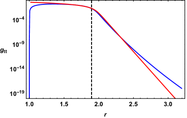
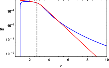
Figure 3: The sudden crossover of the metric component $g_{tt}$ at the would-be Cauchy horizon. The numerical solution of the equations of motion is depicted by the blue curve, while the red line is a fit to the analytic form (18) valid around $r\sim r_{\mathcal{I}}$. Left panel: The Type I model with $\alpha/T=19.8$. Right panel: The Type II case with $K=0.1\sqrt{X}+0.3X$. We have fixed $\alpha/T=24.95$. The location of the would-be inner horizon $r_{\mathcal{I}}$ is denoted by the dashed vertical line.

4 Thermal holographic flows and the Kasner singularity

After studying the internal structure of our hairy black holes as well as the the collapse of the Einstein-Rosen bridge that occurs at the location of $r_{\mathcal{I}}$ of the would-be inner horizon, we now construct the holographic flows sourced by the scalar field $\phi$ and analyze, in particular, the asymptotic behavior near the spacelike singularity.

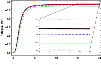
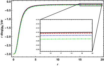
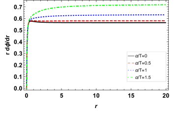
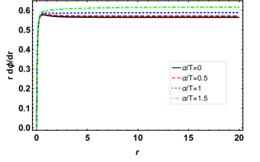
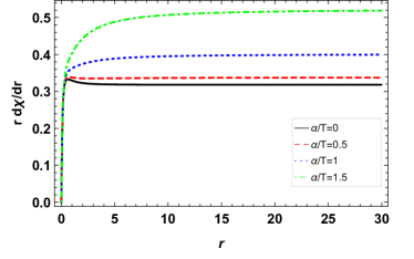
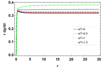
Figure 4: The functions $r\,dX/dr$ with $X=\{\phi,\chi,\log g_{tt}^{\prime}\}$. Left panel: Type I case. Right panel: Type II case with $a_{1}=0.1$ and $a_{2}=0.3$. The solid dark, dotted blue, dashed red, and dotted dashed green curves correspond to $\alpha/T=\{0,0.1,0.5,1\}$, respectively. For these cases, the functions $r\,dX/dr$ tend to be a constant at spacelike singularity. These constants will be determined by the Kasner exponents.

In Fig. 4 we present the behaviors of the various functions approaching the singularity and for different values of $\alpha/T$ by taking $\phi_{0}/T=12.5$ and $V(\phi^{2})=-2\phi^{2}$. The curves therein provide explicit examples of holographic flows that interpolate from a UV radial scaling to a timelike scaling towards a late time singularity behind the black hole event horizon, when the thermal state of the dual CFT is deformed by a relevant scalar operator.

Interestingly, we find that for both type I and type II models, all curves approach to constant values near the singularity as $r\rightarrow\infty$. Actually, we verify numerically (and validate a posteriori) that for our present cases the mass term of the scalar field and the potential $K$ in the equations of motion can be neglected. Assuming that the contributions from the graviton mass (i.e. $\alpha\neq 0$) are negligible, the resulting equations can be solved in generality and the solutions at large $r$ take the following form:

$$\phi=2c\log r+...,\hskip 14.22636pt\chi=4c^{2}\log r+...,\hskip 14.22636ptf=-f_{1}r^{3+2c^{2}}+...\,,$$ (20)

with $c$ and $f_{1}$ constants. Therefore, one finds that the geometry near the singularity takes a Kasner form

$$ds^{2}\sim-d\tau^{2}+\tau^{2p_{t}}dt^{2}+\tau^{2p_{x}}\left(dx^{2}+dy^{2}\right)\,,\hskip 14.22636pt\phi\sim-p_{\phi}\log\tau\,,$$ (21)

where we have traded the radial coordinate $r$ to the proper time $\tau$ via $d\tau=\frac{dr}{r\sqrt{f}}$. The Kasner exponents in Eq.(21) are given by

$$p_{x}=\frac{2}{3+2c^{2}},\hskip 14.22636ptp_{t}=\frac{2c^{2}-1}{3+2c^{2}},\hskip 14.22636ptp_{\phi}=\frac{4c}{3+2c^{2}}\,.$$ (22)

One can immediately verify that the above exponents obey

$$p_{t}+2p_{x}=1,\hskip 14.22636ptp_{\phi}^{2}+p_{t}^{2}+2p_{x}^{2}=1\,.$$ (23)

Before proceeding, let’s consider the case without scalar hair, $\phi=0$. Notice that for this case the contributions from the graviton mass are not negligible and therefore Eq. (20) is not applicable. As evident from Fig. 1, for $\phi=0$, the hairless black hole can have different internal structures, depending on the value of $\alpha$. Taking the Type I potential as an example, for $0\leq\alpha<\sqrt{2}/r_{+}$, the black hole (12) has no inner Cauchy horizon and the interior is similar to the Schwarzschild case with $p_{t}=-1/3$. For $\sqrt{2}/r_{+}<\alpha<\sqrt{6}/r_{+}$, there is a smooth inner horizon which has $p_{t}=1$ in Kasner coordinate. The extremal case $T=0$ is obtained at $\alpha=\sqrt{6}/r_{+}$. Another particular case is $\alpha=\sqrt{2}/r_{+}$ for which there is no inner horizon and $p_{t}=0$.

So far, Fig. 4 proves the existence of the already discussed holographic flows from the AdS boundary to an interior Kasner universe. The emergent Kasner scaling is determined by the two dimensionless CFT parameters $\phi_{0}/T$ and $\alpha/T$. The Kasner exponent $p_{t}$ as function of $\phi_{0}/T$ for different $\alpha/T$ is presented in Fig. 5 from which one can see that $p_{t}$ deviates from $-1/3$ as the source is increased. Therefore, a deformation triggered by the scalar operator changes the near-singularity scaling exponents, signifying a dynamical instability of the singularity for the hairless black hole at later interior time. The Kasner exponent $p_{t}$ with respect to $\alpha/T$ with $\phi_{0}/T$ fixed is shown in Fig. 6. One finds that $p_{t}$ increases monotonically as $\alpha/T$ is increased. Our numerical data can be fitted well by a quadratic form $c_{1}+c_{2}(\alpha/T)^{2}$ with $c_{1}$ and $c_{2}$ constants.

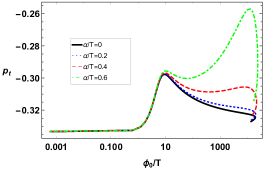
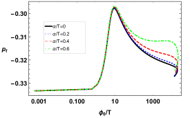
Figure 5: The Kasner exponent $p_{t}$ of the singularity as a function of the dimensionless scalar source $\phi_{0}/T$ for different values of $\alpha/T$. Left panel: Type I case. Right panel: Type II case with $a_{1}=0.1$ and $a_{2}=0.3$. As $\phi_{0}/T$ increases for fixed $\alpha/T$, $p_{t}$ deviates from the value $-1/3$.

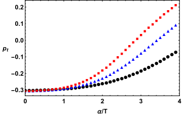
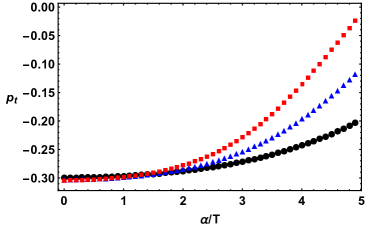
Figure 6: Diagram of the Kasner exponent $p_{t}$ as a function of the parameter $\alpha/T$ for $\phi_{0}/T=\{12.5,15,30\}$ from top to bottom, respectively. Note that the left panel is related to the Type I case with $K=X$, while the right panel is related to the Type II one with $K=a_{1}\sqrt{X}+a_{2}X$ and $a_{1}=0.1$, $a_{2}=0.3$.

In the above discussion, we have required the kinetic term of scalar field to be dominant with respect to the potential terms $V$ and $K$ of (1), or more precisely that

$$\lim_{r\to\infty}\frac{|V(\phi^{2})|}{r^{3+2c^{2}}}\ll 1\hskip 7.11317pt\text{and}\hskip 7.11317pt\lim_{r\to\infty}\frac{|K(\alpha^{2}r^{2})|}{r^{3+2c^{2}}}\ll 1\,.$$ (24)

In particular, the first condition allows the scalar potential to be an arbitrary polynomial functions of $\phi$. However, as pointed out in Cai:2020wrp ; An:2021plu , if one considers a case that diverges exponentially or even worse, the above condition can be violated and the Kasner form would break down.

Before ending this section, we discuss indeed a scenario in which the Kasner form (20) can be violated near the singularity. For illustration, we consider the following form of potentials:

$$V(\phi^{2})=-\phi^{2}-\cosh(\gamma\phi^{2})+1,\quad K(X)=X^{n}\,,$$ (25)

with $\gamma>0$ such that $\frac{\mathrm{d}{V}}{\mathrm{d}{\phi^{2}}}<0$ to remove any inner horizon, and $n>0$ to avoid the ghost and gradient instabilities Baggioli:2014roa . Following Cai:2020wrp , we assume we are in the Kasner regime where one has $\phi=2c\ln r$ at large $r$. For the potentials of (25), we have

$$\frac{|V(\phi^{2})|}{r^{3+2c^{2}}} \sim \frac{e^{4c^{2}\gamma(\ln r)^{2}}}{r^{3+2c^{2}}}>\frac{e^{4c^{2}\kappa\gamma\ln r}}{r^{3+2c^{2}}}=r^{4c^{2}\kappa\gamma-3-2c^{2}}\,,$$ (26)

$$\frac{|K(\alpha^{2}r^{2})|}{r^{3+2c^{2}}} \sim \frac{(\alpha^{2}r^{2})^{n}}{r^{3+2c^{2}}}=\alpha^{2n}r^{2n-3-2c^{2}}\,,$$ (27)

where $\kappa$ is a constant for which one only requires $\kappa<\ln r$. It is obvious that when $\kappa>\frac{3+2c^{2}}{4c^{2}\gamma}$ the the first constraint in Eq. (24) is no longer obeyed. In addition, when $n>\frac{3+2c^{2}}{2}$, the second constraint can be violated as well.

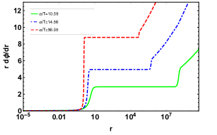
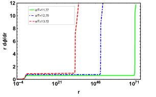
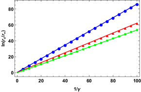
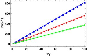
Figure 7: Top panel: The behavior of $rd\phi(r)/dr$ near the singularity for $V(\phi^{2})=-\phi^{2}-\cosh(0.05\phi^{2})+1$. Bottom panel: The relationship between $r_{c}$ and $\gamma$. Here, we select $\phi(r_{h})=0.5$ and $\chi(r_{h})=0$ with $r_{h}=1$ in both cases. Note that the left panels are related to the case Type I with $K=X$, while the right panels are related to the case Type II with $K=a_{1}\sqrt{X}+a_{2}X$ when one takes $a_{1}=0.1$ and $a_{2}=0.3$. The solid lines are the theoretical predictions presented in Eq. (28).

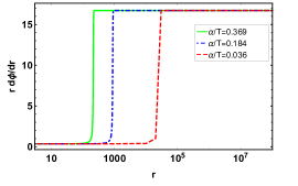
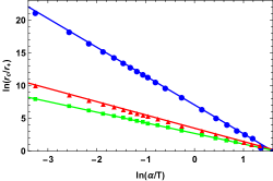
Figure 8: Left: The behavior of $rd\phi/dr$ near the singularity for $V(\phi^{2})=-2\phi^{2}$ and $K(X)=X^{3}$. Right: The relation between the critical point $r_{c}$ and $\ln\alpha$ for different types of massive gravity models $K(X)=\{X^{2},X^{3},X^{4}\}$ from top to bottom, respectively. In all cases, one finds numerically a value of the Kasner constant $c\approx 0.17$ . Here, we select $\phi(r_{h})=0.5$ and $\chi(r_{h})=0$ with $r_{h}=1$ in both cases. The solid lines show the analytical results in Eq. (29).

The above analysis predicts that, for the scalar potential $V$ of Eq. (25), the Kasner form should be violated no matter how small the value of $\gamma$ is. A deviation from the Kasner form is expected beyond a critical point $z_{c}$ given by

$$r_{c}\sim e^{\frac{3+2c^{2}}{4\gamma c^{2}}}\Rightarrow\ln(r/r_{+})=\frac{3+2c^{2}}{4c^{2}\gamma}+b_{\gamma}\,,$$ (28)

with $b_{\gamma}$ a constant. It is numerically challenging to verify the scaling law (28) for small $\gamma$, because one has to solve the equations of motion to sufficiently large $r$. Some examples are shown in Fig. 7 from which one observes a noticeable deviation from the asymptotic solution (20) towards the singularity. The relationship between $r_{c}$ at which the Kasner form is violated and $\gamma$ from our numerics is presented in the bottom of Fig. 7. We indeed verify the expected scaling behavior (28) for small $\gamma$.

We now turn to the role of $K(X)$. Note that for both Type I and Type II, the second constraint of Eq. (24) is always satisfied. In order to see the deviation from the Kasner form, one should consider other forms of $K(X)$. The analysis of (27) suggests to consider $K(X)=X^{n}$ with $n>\frac{3+2c^{2}}{2}$. Consequently, we find a deviation from the Kasner behavior (20) beyond a position $r_{c}$ that obeys

$$\ln\left(\frac{r_{c}}{r_{+}}\right)=-\frac{2n}{2n-(3+2c^{2})}\ln\left(\frac{\alpha}{T}\right)+b_{\alpha}$$ (29)

with $b_{\alpha}$ a constant that depends on the model we take. The case with $K(X)=X^{3}$ is presented in the left panel of Fig. 8 where we numerically show the behavior of $rd\phi/dr$ at the large $r$. As one can see, there exists a critical value $r_{c}$, beyond which the the Kasner behavior will be modified. In the right panel of Fig. 8, we compare the numerical data for $r_{c}$ versus $\alpha$ with our theoretical prediction (29). After fitting the coefficient $b_{\alpha}$, we find that the numerical results agree with the theoretical prediction quite well for all the cases considered, $K(X)=\{X^{2},X^{3},X^{4}\}$.

5 Absence of Josephson oscillations

After studying in detail the geometry and the gravitational dynamics inside the BH horizon in our model, it is time to compare our results with those obtained in Ref. Hartnoll:2020fhc . In their case, before reaching the singularity, strong Josephson oscillations in the condensate are observed. As evident from the previous Sections, this is not the case in our setup; let us explain why. In the previous analysis, we ignored the mass of the scalar field in (17). If we keep the mass term, then the first expression in Eq. (17) takes the following form:

$$\frac{e^{-\frac{\chi}{2}}f}{r^{2}}\Big{(}\frac{e^{-\frac{\chi}{2}}f\phi^{\prime}}{r^{2}}\Big{)}^{\prime}=\frac{|m^{2}g_{tt}|}{r^{4}}\phi\,.$$ (30)

As we have shown, the collapse of the ER brdige occurs in an extremely small range of the $r$ coordinate. Therefore, it is consistent to set $r=r_{\mathcal{I}}$ in Eq. (30). Using this approximation, we obtain the general solution for the scalar field to be

$$\phi=c_{1}e^{\beta\int_{r_{\mathcal{I}}}^{r}e^{\chi/2}/fdr}+c_{2}e^{-\beta\int_{r_{\mathcal{I}}}^{r}e^{\chi/2}/fdr}$$ (31)

where $\beta=\sqrt{|m^{2}g_{tt}(r_{\mathcal{I}})|}$ and $c_{1}$ and $c_{2}$ are integration constants. For the charged scalar case considered in Ref. Hartnoll:2020fhc and using the same coordinates system, the analogous equation of motion reads

$$\frac{e^{-\frac{\chi}{2}}f}{r^{2}}\Big{(}\frac{e^{-\frac{\chi}{2}}f\phi^{\prime}}{r^{2}}\Big{)}^{\prime}=-\frac{q^{2}\Phi^{2}}{r^{4}}\phi$$ (32)

where $q$ and $\Phi$ are respectively the charge of scalar field and the gauge potential. In contrast to (30), in which the coefficient of the right hand side is always positive, the one in Eq. (32) is negative. This is a fundamental difference which will lead to several consequences. In particular, we can solve Eq. (32) and find the oscillating solution discussed in Hartnoll:2020fhc

$$\phi=\phi_{0}\cos\left(|q\Phi(r_{\mathcal{I}})|\int_{r_{\mathcal{I}}}^{r}\frac{e^{\chi/2}}{f}dr+\varphi_{0}\right)\,,$$ (33)

where $\phi_{0}$ and $\varphi_{0}$ are two constants. As the Reader can notice, the difference sign in the r.h.s. of Eq. (30) and Eq. (32) has the important effect of modifying the oscillating solution $\sim e^{\pm ik_{r}r}$ into an exponential one $\sim e^{\pm k_{r}r}$ and therefore makes the Josephson oscillations to disappear.

Notice how the sign of the mass squared $m^{2}$ in our setup is fixed by the requirement of having no inner horizon as discussed in Section 2.2, which concludes our proof for the absence of Josephson oscillations in our case. For completeness, we have verified this fact numerically and we never observed oscillations as expected.

It would be interesting to extend our model by charging the bulk scalar field $\phi$ under a U(1) symmetry. In this case, we do expect a competition between the graviton mass and the effective mass coming from the gauge potential in the superconducting phase. Therefore, at least in some regimes, we do expect the Josephson oscillations to re-appear. In the massive gravity theories considered, holographic superconductor models have been already studied in Baggioli:2015zoa ; Baggioli:2015dwa and they can be directly exploited to answer this question in a more general framework. We leave this new analysis for the future.

6 Probes of the black hole interior and Kasner geometry

In the previous sections, we have shown a rich dynamics in the way the geometry of the BH interior can reach the singularity. For general potentials satisfying the constraint (24), we have found that the deformation of the thermal CFT by a relevant scalar operator leads to a general Kasner universe at late interior times. As these geometrical features should leave strong imprints to all the observable of the dual CFT probing such a region, in this section, we will use several field theory observables to probe the interior of the hairy black holes in the bulk and our previous findings.

The first probe considered is the entanglement entropy. The holographic formula for the entanglement entropy of the dual CFT was proposed in Ryu:2006bv ; Hubeny:2007xt . The entanglement entropy of a subregion $A$ in a $d$ dimensional CFT is given by the minimal area of a bulk co-dimension 2 surface $\gamma_{A}$ homologous to $A$ at the boundary $AdS_{d+1}$ geometry, i.e.

$$S_{A}=\underset{\gamma_{A}}{\text{min}}\frac{\text{Area}(\gamma_{A})}{4G_{N}}\,.$$ (34)

This concept has attracted enormous attention to probe various phase transitions e.g. in black holes Chaturvedi_2016 ; Li:2017gyc ; zeng2016holographic , holographic superconductors Albash:2012pd ; Cai:2012sk ; Cai:2012nm ; Dey_2014 metal-insulator transitions Ling_2016 ; Ling_2017 ; Li_2019 and topological transitions Baggioli:2020cld in the context of the gravity/condensed matter correspondence Takayanagi:2014rue . While formula (34) applies for time-independent case only, a covariant generalization of this formula to general time-dependent case was proposed in Hubeny:2007xt . In this respect, the authors of Hartman:2013qma demonstrated that the extremal surface passes through the interior region of the black brane for early times Hartman:2013qma . Consequently, the growth of the entanglement entropy is related to the growth of the extremal surface along the spacelike surfaces with small curvatures in the interior region of the black brane. At late times, the extremal surface eventually stops expanding on a specific critical surface inside the horizon and does not approach the singularity.

Hence, at late times there is a linear growth in the entanglement entropy with time, from which one defines the entanglement velocity $v_{E}$ Hartman:2013qma :

$$\frac{dS}{dt(0)}=v_{E}\mathcal{V}_{1}s,\quad v_{E}^{2}=r_{+}^{4}\frac{|f|e^{-\chi}}{r^{4}}|_{r=r_{crit}}\,,$$ (35)

where $t(0)$ is the boundary time, $\mathcal{V}_{1}$ is length of $y$ boundary direction  and $s$ is thermal entropy density. For our hairy black holes with a Kasner singularity, $-fe^{-\chi}/r^{4}$ has a maximum inside the horizon at the radius $r_{crit}$. For the black hole solutions (12) and (13), one can obtain $v_{E}$ at small $\alpha/T$ for which the inner horizon is absent and the interior is similar to the Schwarzschild case with $p_{t}=-1/3$.

$$v_{E}=\Bigg{\{}\begin{matrix}\frac{\sqrt{3}}{2\sqrt[3]{2}}-\frac{3\sqrt{3}}{64\pi^{2}}\left(\sqrt[3]{4}-1\right)\left(\frac{\alpha}{T}\right)^{2}+\mathcal{O}\left(\frac{\alpha}{T}\right)^{4}\,,&\hskip 14.22636pt\text{Type I}\\ \frac{\sqrt{3}}{2\sqrt[3]{2}}-a_{1}\frac{\sqrt{3}}{32\sqrt[3]{4}\pi}(2\sqrt[3]{2}-1)\frac{\alpha}{T}+\frac{\sqrt{3}}{4096\pi^{2}}\left(a_{1}^{2}(7-12\sqrt[3]{2}(1-\sqrt[3]{2})\right)\\ -192\,a_{2}(1-\sqrt[3]{4})\left(\frac{\alpha}{T}\right)^{2}+\mathcal{O}\left(\frac{\alpha}{T}\right)^{3}\,.&\hskip 14.22636pt\ \text{Type II}\end{matrix}$$ (36)

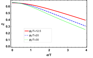
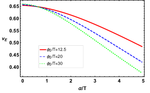
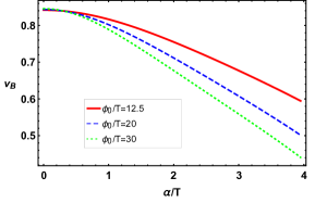
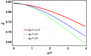
Figure 9: Top: Entanglement velocity $v_{E}$ as a function of $\alpha/T$. Bottom: Butterfly velocity $v_{B}$ as a function of $\alpha/T$. The left panel is for the Type I case with $K=X$, while the right panel for the Type II case $K=a_{1}\sqrt{X}+a_{2}X$ with $a_{1}=0.1$ and $a_{2}=0.3$.

On the other hand, in the context of the gauge/gravity duality, certain properties of quantum chaos in thermal $CFTs$ can be described by the propagation of shock waves near the event horizon of the $AdS$ black hole Shenker:2013pqa ; Roberts_2015 ; Leichenauer_2014 , More precisely, the propagation of the shock wave near the horizon provides a description of the butterfly effect in the dual field theory. The butterfly velocity in terms of bulk quantities is shown to be Shenker:2013pqa

$$v_{B}^{2}=r_{+}\frac{|f^{\prime}|}{4}e^{\chi}\Big{|}_{r=r_{+}}\,.$$ (37)

and it has as well considered as a probe for holographic quantum phase transitions Baggioli:2018afg . For small $\alpha/T$, the butterfly velocity for hairless black hole solutions (12) and (13) are, respectively, given by

$$v_{B}=\Bigg{\{}\begin{matrix}\frac{\sqrt{3}}{2}-\frac{3\sqrt{3}}{128\pi^{2}}\left(\frac{\alpha}{T}\right)^{2}+\mathcal{O}\left(\frac{\alpha}{T}\right)^{4}\,,&\hskip 14.22636pt\text{Type I}\\ \frac{\sqrt{3}}{2}-\frac{\sqrt{3}a_{1}}{32\pi}\frac{\alpha}{T}+\frac{3\sqrt{3}}{1024\pi^{2}}\left(a_{1}^{2}-8a_{2}\right)\left(\frac{\alpha}{T}\right)^{2}+\mathcal{O}\left(\frac{\alpha}{T}\right)^{3}\,,&\hskip 14.22636pt\text{Type II}\\ \end{matrix}$$ (38)

In the presence of the scalar field $\phi$, the black hole interior is deformed. We show the entanglement velocity $v_{E}$ and the butterfly velocity $v_{B}$ as a function of $\alpha/T$ in Fig. 9, and the case as a function of $\phi_{0}/T$ in Fig. 10. One can find that $v_{E}$ and $v_{B}$ display a similar behavior. Both velocities decrease by increasing $\alpha/T$ for given $\phi_{0}/T$. For small $\alpha/T$, both $v_{E}$ and $v_{B}$ as a function of $\phi_{0}/T$ first decrease and then increase, while both decrease monotonically when $\alpha/T$ is large.

Nevertheless, as shown in Fig. 11, the value of butterfly velocity is always bigger than the entanglement velocity, consistent with the result proved in Mezei:2016zxg . By setting $\alpha=0$, our model comes back to the one studied in Frenkel:2020ysx where the hairless background is given by Schwarzschild solution. We find that the ratio $v_{E}/v_{B}$ tends to the Schwarzschild value $v_{E}/v_{B}=1/\sqrt[3]{2}$ as $\phi_{0}/T\to\infty$, which is consistent with the expectation in Frenkel:2020ysx . In contrast, for the massive gravity case ,the ratio $v_{E}/v_{B}$ at large $\phi_{0}/T$ is significantly different from the Schwarzschild value $v_{E}/v_{B}=1/\sqrt[3]{2}$. This suggests that $v_{E}$ and $v_{B}$ can indeed probe the region behind the event horizon. As a property of the black hole interior, we show $v_{E}$ and $v_{B}$ as a function of the Kasner exponent in Fig. 12. For our solutions with a deformed interior, both velocities decrease away from the undeformed values at $-1/p_{t}=3$. As $-1/p_{t}$ is increased, the behaviors are sensitive to the value of $\alpha/T$.

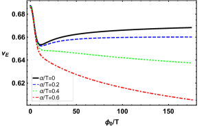
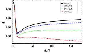
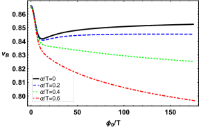
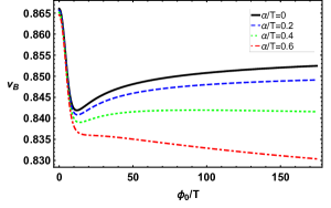
Figure 10: Left: Entanglement velocity $v_{E}$ as a function of $\phi_{0}/T$. Right: the butterfly velocity $v_{B}$ as a function of $\phi_{0}/T$. The left panel corresponds to the Type I case with $K=X$, while the right panel to the Type II case with $K=0.1\sqrt{X}+0.3X$.

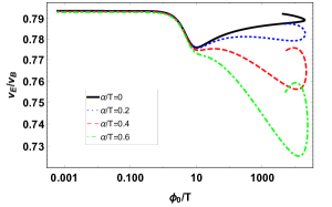
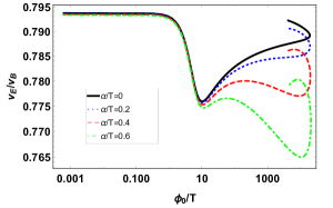
Figure 11: The ratio between $v_{E}$ and $v_{B}$ as a function of $\phi_{0}/T$ by dialing $\alpha/T$. The left panel is for $K=X$, and the right panel for $K=0.1\sqrt{X}+0.3X$.

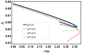
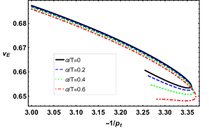
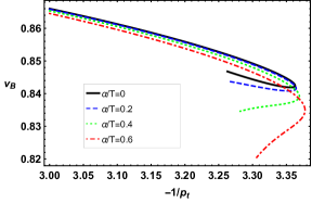
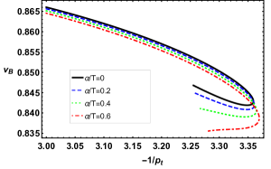
Figure 12: Top: Entanglement velocity $v_{E}$ as a function of $-1/p_{t}$. Bottom: Butterfly velocity $v_{B}$ as a function of $-1/p_{t}$. $K=X$ for the left panel and $K=0.1\sqrt{X}+0.3X$ for the right panel.

7 Conclusions

We have studied holographic RG flows from 3-dimensional UV CFTs to the Kasner universe in the trans-IR driven by a relevant scalar operator in massive gravity theories. In the bulk, this scenario corresponds to black hole solutions at finite temperature with a non-trivial scalar hair $\phi$. Due to the mass of graviton, the black hole in the absence of $\phi$ can have an inner Cauchy horizon, and thus has a similar internal structure of the RN black hole. Nevertheless, we have shown that the Cauchy horizon never develops for any scalar potential with $\frac{\mathrm{d}{V}}{\mathrm{d}{\phi^{2}}}<0$. Therefore, the hairy solution continues smoothly through the event horizon and ends in a spacelike singularity at later interior time. Moreover, we have shown that the instability of the inner horizon results in the collapse of the Einstein-Rosen bridge, for which $g_{tt}$ rapidly collapses to an exponential small value over a shot proper time. We have found that the spacelike singularity takes a general Kasner form as long as the the potentials terms can be neglected. We have also uncovered that the Kasner form can be violated when the potential terms become important to determine the resulting black hole geometry. Finally, we have used the entanglement velocity and butterfly velocity to probe of the black hole interior. In particular, we studied in detail the effect of the scalar deformation and the graviton mass on the Kasner exponents.

In the present work, we have limited ourselves to black holes with maximally symmetric horizons; it would be interesting to consider more general cases with inhomogeneous geometries and with additional matter fields, for example, the case of holographic superconductors. Interestingly, we have shown that the dynamics near the spacelike singularity allows for different behaviors with respect to the standard Kasner form, it is worth investigating this feature in the future in more detail. While both entanglement and butterfly velocities seem to be a property of the black hole interior, they are not able to probe the near-singularity region. It will be helpful to find other probes for the Kasner singularity. Finally, it would be desirable to consider quantum corrections to the interior of black holes, in particular, in the vicinity of the singularity. We hope to report on results in the above directions in the near future.

References

- (1) K. Schwarzschild, On the gravitational field of a mass point according to Einstein’s theory, Sitzungsber. Preuss. Akad. Wiss. Berlin (Math. Phys. ) 1916 (1916) 189–196, [physics/9905030].
- (2) H. Reissner, Über die eigengravitation des elektrischen feldes nach der einsteinschen theorie, Annalen der Physik 355 (1916) 106–120, [https://onlinelibrary.wiley.com/doi/pdf/10.1002/andp.19163550905].
- (3) G. Nordström, On the Energy of the Gravitation field in Einstein’s Theory, Koninklijke Nederlandse Akademie van Wetenschappen Proceedings Series B Physical Sciences 20 (Jan., 1918) 1238–1245.
- (4) R. P. Kerr, Gravitational field of a spinning mass as an example of algebraically special metrics, Phys. Rev. Lett. 11 (Sep, 1963) 237–238.
- (5) R. Penrose, Gravitational Collapse: the Role of General Relativity, Nuovo Cimento Rivista Serie 1 (Jan., 1969) 252.
- (6) S. A. Hartnoll, G. T. Horowitz, J. Kruthoff and J. E. Santos, Gravitational duals to the grand canonical ensemble abhor Cauchy horizons, JHEP 10 (2020) 102, [2006.10056].
- (7) R.-G. Cai, L. Li and R.-Q. Yang, No Inner-Horizon Theorem for Black Holes with Charged Scalar Hairs, JHEP 03 (2021) 263, [2009.05520].
- (8) S. A. Hartnoll, G. T. Horowitz, J. Kruthoff and J. E. Santos, Diving into a holographic superconductor, SciPost Phys. 10 (2021) 009, [2008.12786].
- (9) D. O. Devecioglu and M.-I. Park, No Scalar-Haired Cauchy Horizon Theorem in Einstein-Maxwell-Horndeski Theories, 2101.10116.
- (10) Y.-S. An, L. Li and F.-G. Yang, No Cauchy horizon theorem for nonlinear electrodynamics black holes with charged scalar hairs, Phys. Rev. D 104 (2021) 024040, [2106.01069].
- (11) N. Grandi and I. Salazar Landea, Diving inside a hairy black hole, JHEP 05 (2021) 152, [2102.02707].
- (12) R.-Q. Yang, R.-G. Cai and L. Li, Constraining the number of horizons with energy conditions, 2104.03012.
- (13) J. M. Maldacena, The Large N limit of superconformal field theories and supergravity, Adv. Theor. Math. Phys. 2 (1998) 231–252, [hep-th/9711200].
- (14) L. Fidkowski, V. Hubeny, M. Kleban and S. Shenker, The Black hole singularity in AdS / CFT, JHEP 02 (2004) 014, [hep-th/0306170].
- (15) G. Festuccia and H. Liu, Excursions beyond the horizon: Black hole singularities in Yang-Mills theories. I., JHEP 04 (2006) 044, [hep-th/0506202].
- (16) T. Hartman and J. Maldacena, Time Evolution of Entanglement Entropy from Black Hole Interiors, JHEP 05 (2013) 014, [1303.1080].
- (17) D. Stanford and L. Susskind, Complexity and Shock Wave Geometries, Phys. Rev. D 90 (2014) 126007, [1406.2678].
- (18) A. R. Brown, D. A. Roberts, L. Susskind, B. Swingle and Y. Zhao, Holographic Complexity Equals Bulk Action?, Phys. Rev. Lett. 116 (2016) 191301, [1509.07876].
- (19) A. Frenkel, S. A. Hartnoll, J. Kruthoff and Z. D. Shi, Holographic flows from CFT to the Kasner universe, JHEP 08 (2020) 003, [2004.01192].
- (20) Y.-Q. Wang, Y. Song, Q. Xiang, S.-W. Wei, T. Zhu and Y.-X. Liu, Holographic flows with scalar self-interaction toward the Kasner universe, 2009.06277.
- (21) K. Hinterbichler, Theoretical Aspects of Massive Gravity, Rev. Mod. Phys. 84 (2012) 671–710, [1105.3735].
- (22) V. A. Rubakov and P. G. Tinyakov, Infrared-modified gravities and massive gravitons, Phys. Usp. 51 (2008) 759–792, [0802.4379].
- (23) S. L. Dubovsky, Phases of massive gravity, JHEP 10 (2004) 076, [hep-th/0409124].
- (24) D. Vegh, Holography without translational symmetry, 1301.0537.
- (25) M. Baggioli and O. Pujolas, Electron-Phonon Interactions, Metal-Insulator Transitions, and Holographic Massive Gravity, Phys. Rev. Lett. 114 (2015) 251602, [1411.1003].
- (26) L. Alberte, M. Baggioli, A. Khmelnitsky and O. Pujolas, Solid Holography and Massive Gravity, JHEP 02 (2016) 114, [1510.09089].
- (27) L. Alberte, M. Baggioli and O. Pujolas, Viscosity bound violation in holographic solids and the viscoelastic response, JHEP 07 (2016) 074, [1601.03384].
- (28) L. Alberte, M. Ammon, M. Baggioli, A. Jiménez and O. Pujolàs, Black hole elasticity and gapped transverse phonons in holography, JHEP 01 (2018) 129, [1708.08477].
- (29) L. Alberte, M. Ammon, A. Jiménez-Alba, M. Baggioli and O. Pujolàs, Holographic Phonons, Phys. Rev. Lett. 120 (2018) 171602, [1711.03100].
- (30) M. Baggioli, S. Grieninger and L. Li, Magnetophonons & type-B Goldstones from Hydrodynamics to Holography, JHEP 09 (2020) 037, [2005.01725].
- (31) M. Baggioli, K.-Y. Kim, L. Li and W.-J. Li, Holographic Axion Model: a simple gravitational tool for quantum matter, Sci. China Phys. Mech. Astron. 64 (2021) 270001, [2101.01892].
- (32) T. Andrade and B. Withers, A simple holographic model of momentum relaxation, JHEP 05 (2014) 101, [1311.5157].
- (33) M. Baggioli, Gravity, holography and applications to condensed matter. PhD thesis, Barcelona, Autonoma U., 2016. 1610.02681.
- (34) M. Baggioli, A. Cisterna and K. Pallikaris, Exploring the black hole spectrum of axionic Horndeski theory, 2106.07458.
- (35) M. Ammon, M. Baggioli and A. Jiménez-Alba, A Unified Description of Translational Symmetry Breaking in Holography, JHEP 09 (2019) 124, [1904.05785].
- (36) L. Alberte, M. Ammon, A. Jiménez-Alba, M. Baggioli and O. Pujolàs, Holographic phonons, Physical Review Letters 120 (Apr, 2018) .
- (37) R. A. Davison, Momentum relaxation in holographic massive gravity, Phys. Rev. D 88 (2013) 086003, [1306.5792].
- (38) M. Baggioli and M. Goykhman, Phases of holographic superconductors with broken translational symmetry, JHEP 07 (2015) 035, [1504.05561].
- (39) M. Baggioli and M. Goykhman, Under The Dome: Doped holographic superconductors with broken translational symmetry, JHEP 01 (2016) 011, [1510.06363].
- (40) S. Ryu and T. Takayanagi, Holographic derivation of entanglement entropy from AdS/CFT, Phys. Rev. Lett. 96 (2006) 181602, [hep-th/0603001].
- (41) V. E. Hubeny, M. Rangamani and T. Takayanagi, A Covariant holographic entanglement entropy proposal, JHEP 07 (2007) 062, [0705.0016].
- (42) P. Chaturvedi, V. Malvimat and G. Sengupta, Entanglement thermodynamics for charged black holes, Physical Review D 94 (Sep, 2016) .
- (43) H.-L. Li, S.-Z. Yang and X.-T. Zu, Holographic research on phase transitions for a five dimensional AdS black hole with conformally coupled scalar hair, Phys. Lett. B 764 (2017) 310–317.
- (44) X.-X. Zeng and L.-F. Li, Holographic phase transition probed by non-local observables, 2016.
- (45) T. Albash and C. V. Johnson, Holographic Studies of Entanglement Entropy in Superconductors, JHEP 05 (2012) 079, [1202.2605].
- (46) R.-G. Cai, S. He, L. Li and Y.-L. Zhang, Holographic Entanglement Entropy in Insulator/Superconductor Transition, JHEP 07 (2012) 088, [1203.6620].
- (47) R.-G. Cai, S. He, L. Li and Y.-L. Zhang, Holographic Entanglement Entropy on P-wave Superconductor Phase Transition, JHEP 07 (2012) 027, [1204.5962].
- (48) A. Dey, S. Mahapatra and T. Sarkar, Very general holographic superconductors and entanglement thermodynamics, Journal of High Energy Physics 2014 (Dec, 2014) .
- (49) Y. Ling, P. Liu, C. Niu, J.-P. Wu and Z.-Y. Xian, Holographic entanglement entropy close to quantum phase transitions, Journal of High Energy Physics 2016 (Apr, 2016) 1–9.
- (50) Y. Ling, P. Liu, J.-P. Wu and Z. Zhou, Holographic metal-insulator transition in higher derivative gravity, Physics Letters B 766 (Mar, 2017) 41–48.
- (51) K. Li, M. Han, D. Qu, Z. Huang, G. Long, Y. Wan et al., Measuring holographic entanglement entropy on a quantum simulator, npj Quantum Information 5 (Apr, 2019) .
- (52) M. Baggioli and D. Giataganas, Detecting Topological Quantum Phase Transitions via the c-Function, Phys. Rev. D 103 (2021) 026009, [2007.07273].
- (53) T. Takayanagi, Entanglement entropy and gravity/condensed matter correspondence, Gen. Rel. Grav. 46 (2014) 1693.
- (54) S. H. Shenker and D. Stanford, Black holes and the butterfly effect, JHEP 03 (2014) 067, [1306.0622].
- (55) D. A. Roberts, D. Stanford and L. Susskind, Localized shocks, Journal of High Energy Physics 2015 (Mar, 2015) .
- (56) S. Leichenauer, Disrupting entanglement of black holes, Physical Review D 90 (Aug, 2014) .
- (57) M. Baggioli, B. Padhi, P. W. Phillips and C. Setty, Conjecture on the Butterfly Velocity across a Quantum Phase Transition, JHEP 07 (2018) 049, [1805.01470].
- (58) M. Mezei, On entanglement spreading from holography, JHEP 05 (2017) 064, [1612.00082].