Prospects for detecting exoplanets around double white dwarfs with LISA and Taiji

Abstract

Recently, Tamanini & Danielski (2019) discussed the possibility to detect circumbinary exoplanets (CBPs) orbiting double white dwarfs (DWDs) with the Laser Interferometer Space Antenna (LISA). Extending their methods and criteria, we discuss the prospects for detecting exoplanets around DWDs not only by LISA, but also by Taiji, a Chinese space-borne gravitational-wave (GW) mission which has a slightly better sensitivity at low frequencies. We first explore how different binary masses and mass ratios affect the abilities of LISA and Taiji to detect CBPs. Second, for certain known detached DWDs with high signal-to-noise ratios, we quantify the possibility of CBP detections around them. Third, based on the DWD population obtained from the Mock LISA Data Challenge, we present basic assessments of the CBP detections in our Galaxy during a 4-year mission time for LISA and Taiji. We discuss the constraints on the detectable zone of each system, as well as the distributions of the inner/outer edge of the detectable zone. Based on the DWD population, we further inject two different planet distributions with an occurrence rate of 50% and constrain the total detection rates. We finally briefly discuss the prospects for detecting habitable CBPs around DWDs with a simplified model. These results can provide helpful inputs for upcoming exoplanetary projects and help analyze planetary systems after the common envelope phase.

1 Introduction

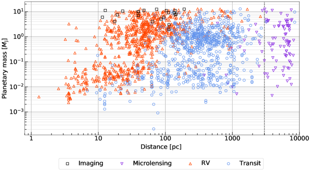
Figure 1: Distribution of planetary mass and distance of the confirmed exoplanets. The black dotted line marks a distance of 3 kpc away from our Solar system. Different markers correspond to the currently known exoplanets using different EM detection techniques. Note that we only plot exoplanets with masses below the deuterium burning limit, i.e. $M_{\mathrm{p}}=13\,M_{\mathrm{J}}$ (see Sec. 3.2). The data were obtained from the NASA Exoplanet Archive.

So far, more than 4,300 exoplanets have been discovered using electromagnetic (EM) techniques, but we know very little about planetary systems under extreme conditions, such as around white dwarfs (WDs). Theoretical works suggest that a planet can survive the host-star evolution (Livio & Soker, 1984; Duncan & Lissauer, 1998; Nelemans & Tauris, 1998), and the observational results also confirm that P-type exoplanets (Dvorak, 1986) can exist around stars after one or two common envelope (CE) phases, for example, around system NN Ser, which contains a WD and a low-mass star (Beuermann et al., 2010, 2011), and PSR B1620$-$26AB, which contains a WD and a millisecond pulsar (Sigurdsson, 1993; Thorsett et al., 1993). Nevertheless, no exoplanets have been discovered orbiting double WDs (DWDs) to date (Tamanini & Danielski, 2019). Given that more than $\sim 97\%$ of stars will become WDs (Althaus et al., 2010) and about 50% of Solar-type stars are not single (Raghavan et al., 2010; Duchêne & Kraus, 2013), there should be a considerable population of DWDs in our Galaxy. If exoplanets do exist around DWDs, the detection of such a population in the future would be very promising.

However, even if exoplanets can endure the CE phase(s), they may collide with each other or be ejected from evolving systems due to the complex orbital evolution (Debes & Sigurdsson, 2002; Veras et al., 2011; Veras & Tout, 2012; Veras, 2016; Mustill et al., 2018). Strong tidal forces can crush the planetary cores during their migration or scattering processes (Farihi et al., 2018), which may be associated with the WD pollution effect (Jura et al., 2009; Farihi, 2016; Brown et al., 2017; Smallwood et al., 2018). Therefore, as noted by Danielski et al. (2019), the detection and study of these objects can help analyze planetary systems after CE phases and the planetary formation processes.

Owing to the intrinsic faintness of DWDs and the sensitivity limits of the current EM methods, there are no more than 200 known detached DWD systems (Brown et al., 2020). The amount of known interacting (AM CVn) DWD systems is even fewer (Ramsay et al., 2018). A more frustrating fact is that most detected exoplanets are restricted to the Solar neighborhood ($\sim 3$ kpc) and discovered successfully by EM detection methods (see Fig. 1), such as radial velocity (RV) and transit measurements. Gravitational microlensing is capable of detecting exoplanets farther away ($\sim 8$ kpc) towards the Galactic bulge, but scarcity and unrepeatability can be two of the main restricting factors. All these show that it is hard to discover exoplanets orbiting DWDs using traditional EM techniques in the Milky Way (MW).

Differently, gravitational waves (GWs) can provide a powerful tool in the detection of exoplanets beyond our Solar system without the above selection problem (Seto, 2008; Wong et al., 2019). Recent studies have explored the prospects for detecting new circumbinary exoplanets (CBPs) around DWDs in our Galaxy by using the Laser Interferometer Space Antenna (LISA) mission (Tamanini & Danielski, 2019; Danielski et al., 2019). The method, measuring the perturbation on the GW signals due to CBPs, is conceptually similar to the RV technique. Compared to the traditional EM methods, GW detections are able to detect such a CBP population in principle everywhere in the MW without being affected by stellar activities, which, in contrast, should be considered rather carefully in EM observations. An even more exciting prospect is that space-borne GW detectors have the potential to detect DWDs in nearby galaxies (Korol et al., 2020; Roebber et al., 2020), up to the border of the Local Group (Korol et al., 2018). From these we can see that in the near future, considering the rapid development of GW astronomy, the first ever extra-galactic planetary system might be detected by the space-borne GW detectors (Danielski & Tamanini, 2020).

In this paper, firstly, we followed the method and procedure presented in Tamanini & Danielski (2019) to discuss the prospects for detecting CBPs around DWDs by using two different space-borne GW detectors, LISA and Taiji. We give a complementary discussion on the possibility of CBP detections around some known detached DWDs with high signal-to-noise ratios (SNRs). Secondly, based on the DWD population from the Mock LISA Data Challenge (MLDC) Round 4 (Babak et al., 2010), we explore the population of CBP detections in our Galaxy during a 4-year mission time for GW detectors. For comparison, recent work has used dedicated binary synthesis simulations for the DWD population (Korol et al., 2017; Lamberts et al., 2019), and our results are remarkably consistent with them, yet providing a faster way for assessments. Thirdly, we introduce detectable zone for each promising detectable system and discuss the distributions of the inner/outer edge of this area. Fourthly, we inject two different planet distributions with an occurrence rate of 50% for DWDs to constrain the total detection rate during a 4-year mission time. Finally, we briefly discuss the prospects for detecting habitable CBPs around DWDs with a simplified model by assuming that the habitable zone boundary criteria for main-sequence (MS) stars also apply to DWDs. These results can provide a crude benchmark for upcoming exoplanetary projects and help analyze planetary systems after CE phases.

The organization of this paper is as follows. We briefly introduce the two space-borne GW detectors that we use and the construction of their sensitivity curves in Sec. 2. In Sec. 3, we overview the method proposed in Tamanini & Danielski (2019), and present the characteristics of DWD populations and CBP models used in our work for LISA and Taiji. Using the above ingredients, we report detailed analyses and our results on various aspects of CBP detections in Sec. 4. Finally, we present a conclusion in Sec. 5.

2 Detectors

The era of GW astronomy has begun since the first direct detection of GWs, namely GW150914 (Abbott et al., 2016). Generally, the ground-based GW detectors are sensitive to frequencies between $\sim 10$ Hz and a few of kHz, which has made them succeed in “listening” to numerous GWs from merging stellar-mass sources, like binary black holes and binary neutron stars (Abbott et al., 2017). For the space-borne detectors, such as LISA and Taiji, the sensitive frequency band ranges from 0.1 mHz to 1 Hz due to their much longer arm lengths and specific optics. In such a frequency range, the potential GW signals come from different sources, and are considered to have great astronomical and cosmological significances (Cutler & Thorne, 2002; Berti et al., 2005; Klein et al., 2016; Shi et al., 2019). In particular, Galactic binaries including DWDs are one class of the prominent sources emitting continuous GWs in this frequency band.

2.1 LISA and Taiji

LISA mission, proposed by an international collaboration of scientists called the LISA Consortium, is an ESA-led L3 mission, with NASA as a junior partner, to record and study gravitational radiation in the millihertz frequency band (Amaro-Seoane et al., 2017). It consists of three spacecrafts with $2.5\times 10^{6}$ km arm-lengths trailing the Earth and moving in the Earth orbit around the Sun. In the sensitive frequency range of LISA, the dominant GW sources by numbers will be Galactic DWDs in the MW (Lamberts et al., 2019). So for any CBPs orbiting DWDs, LISA would be a promising tool to indirectly detect them. As mentioned in Sec. 1, the potential of LISA to detect the first extra-galactic planetary was discussed by Danielski & Tamanini (2020).

On the other hand, Taiji, whose prototype was started in 2008, is a Chinese space-borne GW mission similar to LISA. It also consists of three satellites forming a giant equilateral triangle, but with $3\times 10^{6}$ km arm-lengths, slightly longer than that of LISA (Luo et al., 2020; Ruan et al., 2020; Wang & Han, 2021). These satellites are planned to orbit the Sun in the Earth orbit with approximately 20 degrees ahead of the Earth. Taiji also aims to detect low-frequency GW sources in the frequency band between 0.1 mHz to 1 Hz. Its sensitivity curve at the lower frequency range performs slightly better than LISA, thus, as we will see, it has advantages on the detection of DWDs and CBPs.

2.2 Sensitivity curves

When it comes to GW detectors, sensitivity curves are important performance guidelines. We can use them as a tool to evaluate what types of sources can be detected during the mission. As described in Robson et al. (2019), we know that the sensitivity of GW detectors depends on the GW frequency $f$, as given by

$$\begin{split}S_{n}(f)=&\frac{10}{3L^{2}}\left[P_{\mathrm{OMS}}+2\left(1+\cos^{2}\left(f/f_{*}\right)\right)\frac{P_{\mathrm{acc}}}{(2\pi f)^{4}}\right]\\ &\times\left[1+\frac{6}{10}\big{(}\frac{f}{f_{*}}\big{)}^{2}\right]+S_{c}(f)\,,\end{split}$$ (1)

where $S_{n}(f)$ is referred to as the effective noise power spectral density; $L$ is the arm length of space-borne GW detector; $f_{*}=c/(2\pi L)$ is called the transfer frequency. Due to the longer arm length of Taiji ($L=3\times 10^{6}$ km), $f_{*}$ is a little smaller for Taiji than for LISA ($L=2.5\times 10^{6}$ km). In the expression above, the single-link optical metrology noise is quoted as $P_{\mathrm{acc}}$, while the single test-mass acceleration noise $P_{\mathrm{OMS}}$ is slightly different between the two missions. More details and analyses of these parameters can be found in Robson et al. (2019) and Wang & Han (2021).

Besides the instrument noise, estimates for the confusion noise $S_{c}(f)$ are also very important. $S_{c}(f)$ is caused by the unresolved Galactic binaries, and it is associated with the design of the space-borne detectors. As described in Robson et al. (2019), estimates for $S_{c}(f)$ are well fit by

$$\begin{split}S_{c}(f)=&A_{\mathrm{fix}}f^{-7/3}\mathrm{e}^{-f^{\alpha}+\beta f\sin(\kappa f)}\\ &\times\big{[}1+\tanh\big{(}\gamma(f_{k}-f)\big{)}\big{]}\mathrm{Hz}^{-1}\,,\end{split}$$ (2)

where the fixed amplitude $A_{\mathrm{fix}}=9\times 10^{-45}$, the knee frequency $f_{k}=0.00113$ and other fit parameters are given for a 4-year observational time as $\alpha=0.138$, $\beta=-221$, $\kappa=521$, and $\gamma=1680$. We plot the sensitivity curves of LISA and Taiji in terms of their characteristic strain, $\sqrt{fS_{n}(f)}$, in Fig. 2. Note that we have assumed a 4-year nominal mission duration for all the discussions throughout this paper. The curve of Taiji taken from Luo et al. (2020) is combined with $S_{c}(f)$, which we assume to be approximately the same for LISA and Taiji due to their similar designs and configurations. In reality, as the noise in the low-frequency band for Taiji is slightly better for LISA, such an assumption puts us being conservative for Taiji’s performance, as Taiji will be able to distinguish more Galactic binaries at these frequencies. Future studies could refine this point.

3 method

As mentioned in the Introduction, the GW method for detections of CBPs was firstly proposed by Tamanini & Danielski (2019). This approach relies on the large DWD population with orbital periods $\lesssim 1$ hour, which are expected to be the most numerous GW sources for space-based mHz GW detectors (Nelemans et al., 2001; Yu & Jeffery, 2010; Amaro-Seoane et al., 2017; Lamberts et al., 2018; Breivik et al., 2020). Because of the richness of potential sources, GWs could be a powerful tool to detect CBPs around DWDs. In this section, we will present our methodology to analyze the problem, which extends the original one in Tamanini & Danielski (2019). In Sec. 3.1, we describe how we obtain the DWD population with some reasonable assumptions. In Sec. 3.2, we provide some details about the CBP injection process. The method for the GW detection of CBPs is discussed in Sec. 3.3.

3.1 DWD population

We consider systems that compose of an exoplanet around a DWD. For such three-body systems, there is no doubt that the gravity of DWDs dominate the GW signal when compared with that of exoplanets. Therefore, we provide quantitative estimates and constraints for the detection of CBPs in our Galaxy based mainly on the population of DWDs. To give quick assessments, we obtain the DWD population from the MLDC Round 4, which is designed to demonstrate and encourage the analysis of different GW sources (Babak et al., 2010). MLDC Round 4 includes a Galactic DWD population with $\sim 3.4\times 10^{7}$ interacting binaries and $\sim 2.6\times 10^{7}$ detached ones. We abandon the population of the interacting systems mainly for two reasons: (i) the chirp masses of the accreting systems are hard to obtain with GW observations only, and (ii) accreting effects would complicate our analysis of CBPs. Such a treatment was adopted in previous work as well (Tamanini & Danielski, 2019; Danielski et al., 2019), and we leave the accreting systems for future studies.

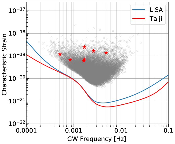
Figure 2: Characteristic strains of the detached DWD population, whose SNR $>10$ for Taiji, are plotted with grey circles. The known detached DWDs with high SNRs (listed in Table 3 and discussed in Sec. 4.2.1) are highlighted with red stars. Note that the DWD population is plotted based on a crude assumption that two WDs are equal in mass. We also plot the sensitivity curves of LISA (blue line) and Taiji (red line) as given in Sec. 2.2.

Different values of DWD parameters not only lead to different SNRs, but also change the estimations of detecting abilities. This was analyzed in Tamanini & Danielski (2019). We will also discuss the detecting abilities with different values of mass and mass ratio in Sec. 4.1. When we perform the calculations to assess the prospects of the final CBP detections in the MW, we acquire the parameters of each binary from the dataset, including the GW frequency $f$, the frequency derivative $\dot{f}$, the ecliptic latitude $\beta$, the ecliptic longitude $\lambda$, the GW amplitude $\mathcal{A}$, the inclination $\iota$, and the polarization phase $\psi$. More details of the population and the parameters are presented in Babak et al. (2008, 2010). As we will see later in Sec. 3.3.1, we can derive the chirp mass $\mathcal{M}$ of each system through the use of observed GW frequency $f$ and its time derivative $\dot{f}$. By assuming that the two WDs are almost equal in mass, we can then acquire the mass of each WD pair, ($m_{1}$,$m_{2}$), and their total mass $M_{\mathrm{b}}\equiv m_{1}+m_{2}$. We regard this as a crude but reasonable treatment because the mass ratio $q=m_{1}/m_{2}$ ($m_{1}>m_{2}$) under discussion is often considered lower than 3 for detected DWDs (for example, see e.g. Korol et al., 2017). In Sec. 4.1, we will show little differences in detecting abilities when realistic mass ratio is considered.

With the above consideration, we re-calculate the SNRs of 31,530 “bright” detached Galactic binaries from MLDC Round 4 for the two detectors. We find that approximately $2.9\times 10^{4}$ ($2.2\times 10^{4}$) detached DWDs have $\mathrm{SNR}>7$ for Taiji (LISA) during a 4-year mission. The number becomes $2.5\times 10^{4}$ ($1.6\times 10^{4}$) for $\mathrm{SNR}>10$. For the following, we filter out all detached binaries with $\mathrm{SNR}<10$, for both LISA and Taiji, to get more reliable estimations and striking contrasts between the two missions in detecting abilities. Also, a high SNR is generally needed in order to have CBP detections around DWDs. In Fig. 2 we show the dimensionless characteristic strain of the detached DWD population with $\mathrm{SNR}>10$ for Taiji. Because of the direct use of the DWD catalog, we could provide faster assessments for comparisons which are consistent with previous work within an order of magnitude (Korol et al., 2017; Lamberts et al., 2019; Danielski et al., 2019).

3.2 Injection of CBP models

When we consider CBPs around a DWD, there is no evidence to claim that every DWD should have such an exoplanet. Given that no planets have been discovered orbiting DWDs so far, we take a bold approach, following Danielski et al. (2019), and set 50% as the occurrence rate for our synthetic population of CBPs around DWDs, which is obtained according to the observed frequency of WD pollution effect (Koester et al., 2014). Note also that even if such CBPs exist, we may miss these exoplanets using space-borne GW detectors for a variety of reasons. Therefore, a combination of diverse semi-major axis ($a$) and CBP mass ($M_{\mathrm{p}}$) distributions have been tested in Danielski et al. (2019), from which we adopt the optimistic and the pessimistic cases as reference points. Notice that there is a difference between the distributions in Danielski et al. (2019) and ours in the planet’s orbital inclination $i$. Instead of setting a uniform distribution in $\cos i$, we inject CBPs into the DWD systems by assuming coplanar circular orbits. There are theoretical indications that CBPs prefer to be coplanar with their central binaries (Kennedy et al., 2012; Foucart & Lai, 2013), and coplanar orbits have been considered in various other work as well (Dvorak, 1986; Holman & Wiegert, 1999; Eberle et al., 2008; Hong & van Putten, 2021). It is certainly advantageous to refine the currently quite uncertain CBP population models in future for more accurate predictions, in particular for a realistic estimate via the GW method. We will show more details and our detection rates in Sec. 4.2.3.

3.3 Detection of CBPs around DWDs

This subsection briefly introduces the method for the GW detection of a CBP using space-borne GW detectors. We follow Tamanini & Danielski (2019) to model the perturbation induced by CBPs around DWDs. We first describe some characteristics of the three-body system in Sec. 3.3.1, and then provide more details about the parameter estimation process in Sec. 3.3.2.

3.3.1 Perturbation due to a CBP

Considering a three-body system composed of a DWD emitting GWs with an exoplanet on the outer orbit (P-type system), we assume that the separation between the planet and the DWD is much greater than the separation between the two WDs. For simplicity, we also consider both these orbits as circular Keplerian orbits. This could root in the binary evolution scenarios. Based on these assumptions, we obtain the radial velocity of the DWD with respect to the common center of mass (CoM),

$$v_{\mathrm{rad}}(t)=-K\cos\varphi(t)\,.$$ (3)

We have defined,

$$K =\Big{(}\frac{2\pi G}{P}\Big{)}^{1/3}\frac{M_{\mathrm{p}}}{\left(M_{\mathrm{b}}+M_{\mathrm{p}}\right)^{2/3}}\sin i\,,$$ (4)

$$\quad\varphi(t) =\frac{2\pi t}{P}+\varphi_{0}\,,$$ (5)

where $P$ and $i$ are respectively the orbital period and inclination of the CBP, $\varphi(t)$ is the outer orbital phase, and $\varphi_{0}$ is its initial value at $t=0$.

Through the Doppler effect, the observed GW frequency changes in the Earth reference frame to,

$$f_{\mathrm{obs}}(t)=\left(1+\frac{v_{\mathrm{rad}}(t)}{c}\right)f_{\mathrm{GW}}(t)\,,$$ (6)

where $f_{\mathrm{GW}}(t)$ is the GW frequency in the DWD reference frame (twice the DWD orbital frequency). Galactic binaries take much longer than the mission time of GW detectors to merge, and their frequencies are changing very slowly. We can then describe their time evolution with a Taylor expansion and neglect the second and higher-order terms by using,

$$f_{\mathrm{GW}}(t)=f+\dot{f}t+O\left(t^{2}\right)\,,$$ (7)

where $f$ is the initial observed GW frequency, and $\dot{f}$ is its time derivative, which are related to the chirp mass $\mathcal{M}=(m_{1}m_{2})^{3/5}/(m_{1}+m_{2})^{1/5}$ of the DWD system via,

$$\dot{f}=\frac{96}{5}\pi^{8/3}f^{\ 11/3}\left(\frac{G\mathcal{M}}{c^{3}}\right)^{5/3}\,.$$ (8)

Finally, by integrating the observed GW frequency $f_{\mathrm{obs}}(t)$, we can obtain the phase at the observer of the GWs,

$$\Psi_{\mathrm{obs}}(t)=2\pi\int f_{\mathrm{obs}}\left(t^{\prime}\right)dt^{\prime}+\Psi_{0}\,,$$ (9)

where $\Psi_{0}$ is the constant initial phase. The final form of the observed phase is given by,

$$\begin{split}\Psi_{\mathrm{obs}}(t)=&2\pi\Big{(}f+\frac{1}{2}\dot{f}t\Big{)}t-\frac{Pf}{c}K\sin\varphi(t)\\ &-\frac{P\dot{f}t}{c}K\sin\varphi(t)-\frac{P^{2}\dot{f}}{2\pi c}K\cos\varphi(t)\,.\end{split}$$ (10)

With all the equations above, the parameters characterizing the DWD and the perturbation induced by a CBP can thus be extracted from the GW phase evolution.

3.3.2 Parameter estimation for LISA and Taiji

In low frequency range, LISA and Taiji each can be effectively seen as a pair of two-arm GW detectors like LIGO and Virgo, and output two linearly independent signals, $h_{\mathrm{I}}(t)$ and $h_{\mathrm{II}}(t)$. We often assume that the noise is stationary and Gaussian, and then the two signals in each independent channel can be written as (Cutler, 1998),

$$h_{\mathrm{I,II}}(t)=\frac{\sqrt{3}}{2}A_{\mathrm{I,II}}(t)\cos\big{[}\Psi_{\mathrm{obs}}(t)+\Phi_{\mathrm{I,II}}^{\mathrm{p}}(t)+\Phi_{\mathrm{D}}(t)\big{]}\,,$$ (11)

where $A_{\mathrm{I,II}}(t)$ are amplitudes of GW signals that contain the constant intrinsic amplitudes of the waveform and the antenna pattern functions of the detector. In our case the waveform is approximated by a circular Newtonian binary. The antenna pattern functions are related to geometric parameters, including the location of the source ($\theta_{S},\phi_{S}$), the orientation of the DWD orbit ($\theta_{L},\phi_{L}$), and the configuration of the space-borne detector. In Eq. (11), $\Phi_{\mathrm{I,II}}^{\mathrm{p}}(t)$ are the waveform’s polarization phases induced by the change of the orientation of the detector. The Doppler phase $\Phi_{\mathrm{D}}(t)$ is the difference between the phase of the wavefront at the detector and the phase of the wavefront at the Sun. It is further related to the Earth-Sun distance and the orbital period of the Earth. The full expressions for all above quantities can be found in Cutler (1998), Cornish & Larson (2003), and Korol et al. (2017).

Based on the above analysis, our next step is to simulate the response of LISA and Taiji and perform parameter estimation. We use the Fisher information approach, as was employed by Tamanini & Danielski (2019). For each DWD, there are 11 parameters, $\boldsymbol{\lambda}=\big{\{}\ln(A),\Psi_{0},f,\dot{f},\theta_{S},\phi_{S},\theta_{L},\phi_{L},K,P,\varphi_{0}\big{\}}$, characterizing the observed GW waveform. The Fisher matrix can be written as

$$\Gamma_{ij}=\frac{2}{S_{n}\left(f\right)}\sum_{\alpha=\mathrm{I,II}}\int_{0}^{T_{\mathrm{obs}}}\left(\frac{\partial h_{\alpha}(t)}{\partial\lambda_{i}}\cdot\frac{\partial h_{\alpha}(t)}{\partial\lambda_{j}}\right)dt\,.$$ (12)

We use the one-sided noise power spectral density $S_{n}(f)$ of the detector from Eq. (1). For each DWD, it is merely a constant in Eq. (12) because the binary is quasi-monochromatic during the observational time $T_{\mathrm{obs}}$ as long as $\dot{f}T_{\mathrm{obs}}\ll f$.

Similarly, the SNR of the signal can be written as,

$$\mathrm{SNR}=\bigg{(}\frac{2}{S_{n}\left(f\right)}\sum_{\alpha=\mathrm{I,II}}\int_{0}^{T_{\rm obs}}h_{\alpha}(t)h_{\alpha}(t)\,dt\bigg{)}^{1/2}\,.$$ (13)

This allows us to scale all results with the SNR by rescaling $S_{n}(f)$ (Tamanini & Danielski, 2019). From the inverse of the Fisher matrix, we can obtain the uncertainties and correlations of parameters as the elements of the variance-covariance matrix $\Sigma_{ij}$,

$$\Sigma_{ij}=\left\langle\Delta\lambda_{i}\Delta\lambda_{j}\right\rangle=\left(\Gamma^{-1}\right)_{ij}\,.$$ (14)

Cutler (1998) has studied the uncertainties for binary parameters. We follow his method and determine different partial derivatives of $\Psi_{\mathrm{obs}}(t)$. Since the error $\Delta\dot{f}$ would be much larger than the signal’s $\dot{f}$ itself, we adopt a treatment to simply set the fiducial value $\dot{f}=0$ without introducing noticeable changes (Takahashi & Seto, 2002). Here we only show expressions of the partial derivatives differing from the equations in the Sec. IV of Cutler (1998),

$$\begin{split}\partial_{K}\Psi_{\mathrm{obs}}(t)&=-\frac{Pf}{c}\sin\varphi(t)\,,\\ \partial_{P}\Psi_{\mathrm{obs}}(t)&=-\frac{f}{c}K\sin\varphi(t)+\frac{2\pi ft}{cP}K\cos\varphi(t)\,,\\ \partial_{f}\>\Psi_{\mathrm{obs}}(t)&=2\pi t-\frac{P}{c}K\sin\varphi(t)\,,\\ \partial_{\dot{f}}\>\Psi_{\mathrm{obs}}(t)&=\pi t^{2}-\frac{Pt}{c}K\sin\varphi(t)-\frac{P^{2}}{2\pi c}K\cos\varphi(t)\,,\\ \partial_{\varphi_{0}}\Psi_{\mathrm{obs}}(t)&=-\frac{Pf}{c}K\cos\varphi(t)\,.\end{split}$$ (15)

To measure the additional perturbation due to an exoplanet, Tamanini & Danielski (2019) paid more attention to the three parameters associated with the CBP, namely $K,P,\varphi_{0}$. Since the value of $\varphi_{0}$ is not important for our final results, we fix $\varphi_{0}=\pi/2$. We set 30% to be the detection criterion on both $\Delta K/K$ and $\Delta P/P$, meaning that a detectable CBP is defined with estimated parameter precision being better than this value.

4 Results

Now we give detailed analyses and discuss the prospects for detecting exoplanets around DWDs. Using Taiji as a demonstration, we first give some complementary discussion on the detecting abilities with different values of masses in Sec. 4.1. We compare our final results of the CBP detection between LISA and Taiji in Sec. 4.2.

4.1 Effects of masses

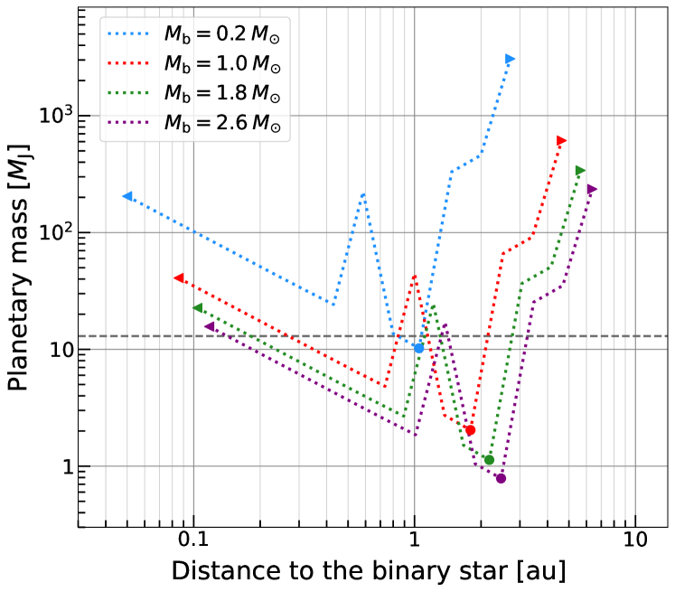
Figure 3: Selection functions of Taiji in the mass-separation parameter space for exoplanets. Four dotted lines in different colors denote systems with different total masses. The dashed horizontal grey line corresponds to the deuterium burning limit $M_{\mathrm{p}}=13$ $M_{\mathrm{J}}$. Circles are the detectable minimum planetary masses for each system, and left/right triangles denote the boundary values we set. The peak of each three-body system is caused by the degeneracy between the motion of Taiji and the motion of the DWD around the three-body CoM.

From Eq. (4), we can see that when other parameters related to the CBP are fixed, such as its angular position and the distance, the perturbation $K$ caused by the exoplanet is getting smaller with the increase of the total mass $M_{\mathrm{b}}$. Meanwhile, the SNR will be in contrast higher when we only increase the total mass of the DWD. Therefore, to give a quantitative evaluation, we perform parameter estimation on the same set of systems except that their total masses are ranging from 0.2 ${M}_{\odot}$ to 2.8 ${M}_{\odot}$. We assume two WDs are equal in mass and fix the other parameters of the DWD as

$$\Psi_{0}=0\,,\quad\theta_{S}=1.27\,,\quad\varphi_{S}=5\,,\quad i=\iota=\frac{\pi}{3}\,.$$ (16)

The frequency and distance of the system are fixed to $f=5$ $\mathrm{mHz}$ and $d_{\mathrm{DWD}}$ = 10 kpc respectively. Note that we derive the orientation of its orbit ($\theta_{L},\varphi_{L}$) by inversing Eq. (39) and Eq. (40) in Cornish & Larson (2003).

We plot for comparison in Fig. 3 the selection functions of Taiji based on these values. The four dotted lines in different colors denote DWDs with different total masses, and the dashed horizontal grey line denotes the deuterium burning limit $M_{\mathrm{p}}=13$ $M_{\mathrm{J}}$, which is considered to be the upper limit of the CBP mass (Danielski et al., 2019). Therefore, it is the area above the dotted lines and below the dashed line that delimits the detectable mass-separation parameter space of the CBP for Taiji. The peak of each line is caused by the degeneracies between the motion of Taiji, and the motion of the DWD in the three-body system around its common CoM (see the section “Methods” in Tamanini & Danielski, 2019). Sharp peaks appear at $P=1$ yr (the orbital period of Taiji), while there are also other smaller peaks at higher harmonics of it.

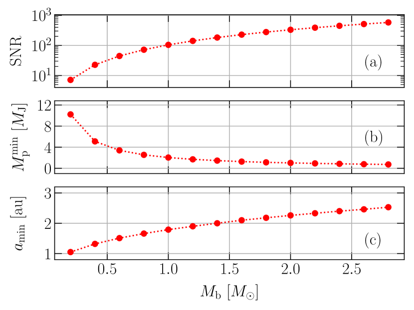
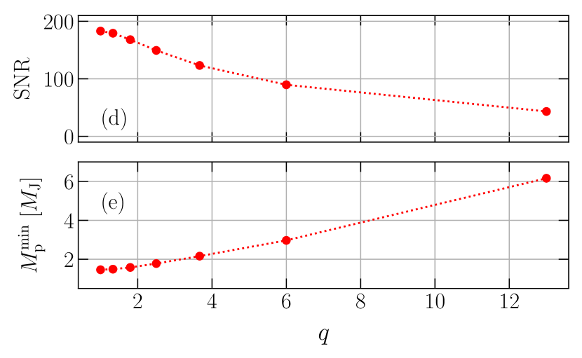
Figure 4: (a) The SNR, (b) the detectable minimum planetary mass, and (c) its corresponding orbital size, as functions of the total mass for equal-mass DWDs. (d) The SNR and (e) the detectable minimum planetary mass, as functions of the mass ratio $q$ for DWDs with a total mass $M_{\rm b}=1.4\,M_{\odot}$. More details about the parameters are given in Sec. 4.1.

For each system, we have fixed the range of the CBP orbital period to $P=0.025$–$10$ yr, and calculated the CBP’s distance to the CoM by Kepler’s third law,

$$a^{3}=\frac{GP^{2}}{4\pi^{2}}(M_{\mathrm{b}}+M_{\mathrm{p}})\,.$$ (17)

We mark the distance boundaries as the left and right triangles in Fig. 3. When the period of the CBP is set to a same value, the planetary orbital size gets larger with the increase of the total mass of the DWD. We find that detecting abilities of each system are gradually getting better with the increasing CBP period before becoming worse near the period of one year. There must be a minimum value $M_{\mathrm{p}}^{\mathrm{min}}$ that corresponds to the detectable minimum planetary mass for each system, which we denote by circles in Fig. 3.

Table 1: Possible detections of CBPs around known DWDs. For each system, $a_{\mathrm{min}}$ is the detectable minimum planetary orbital size based on our parameter estimation. Through the comparative results of LISA and Taiji, we list the detectable minimum planetary mass $M_{\mathrm{p}}^{\mathrm{min}}$ with the SNR for each DWD. For each promising system, we calculate the IDZ and ODZ. Other relevant properties of these known detached DWDs are in the Appendix.

			Taiji					LISA
Source	$a_{\mathrm{min}}$		$M_{\mathrm{p}}^{\mathrm{min}}$		IDZ	ODZ	SNR		$M_{\mathrm{p}}^{\mathrm{min}}$		IDZ	ODZ	SNR
	[au]		[$M_{\mathrm{J}}$]		[au]	[au]			[$M_{\mathrm{J}}$]		[au]	[au]
ZTF J153932.16+502738.8	1.	53	1.	39	0.20	2.20	124.	51	2.	11	0.32	2.12	81.	89
SDSS J065133.34+284423.4	1.	79	2.	34	0.31	2.04	117.	18	2.	95	0.49	2.00	92.	83
SDSS J093506.92+441107.0	2.	03	4.	76	0.73	2.21	139.	66	9.	50	1.40	2.12	70.	02
SDSS J232230.20+050942.06	1.	59	10.	47	1.35	1.66	70.	72	21.	27	–	–	34.	82
PTF J053332.05+020911.6	1.	63	17.	94	–	–	29.	09	37.	69	–	–	13.	84
SDSS J163030.58+423305.7	1.	72	104.	33	–	–	12.	38	283.	92	–	–	4.	55
SDSS J092345.59+302805.0	2.	06	179.	01	–	–	11.	61	412.	89	–	–	5.	03

Moreover, we can see that the detectable parameter space is getting wider with the increase of the total mass of a binary, and the detectable minimum planetary mass is getting smaller. We point out that this can be explained by the parameter estimation criterion on $K$, since in most cases the 30% criterion is not applicable for $\Delta P/P$, as we can see in the Fig. 2 of Tamanini & Danielski (2019). Eq. (4) tells us that the amplitude $K\propto M_{\mathrm{b}}^{-2/3}$. After plugging it into Eq. (12) and Eq. (14), we get $\Delta K\propto M_{\mathrm{b}}^{-5/3}$. Therefore, the detectable minimum planetary masses limited by $\Delta K/K$ are inversely proportional to the total masses of DWDs. We also find similar results in the upper panels of Fig. 4 with a wider range of $M_{b}$ from 0.2 $M_{\odot}$ to 2.8 $M_{\odot}$. From these we conclude that SNR is the dominating factor in detecting abilities when we change the total mass of the DWD. Note that we choose 2.8 $M_{\odot}$ to be the upper limit in this section because we notice that the maximum total mass can reach 2.8 $M_{\odot}$ when we considered a Galactic DWD population from MLDC Round 4 with an equal-mass assumption in the following sections. Although 2.8 $M_{\odot}$ may be too high to be the upper limit for most DWDs, whose total masses usually do not exceed 2 $M_{\odot}$ (Lamberts et al., 2019), it would not alter the qualitative conclusions derived here.

Similarly, by changing the mass ratio $q$ with a fixed total mass $M_{\rm b}=1.4\,M_{\odot}$ of the DWD, we illustrate our results in the lower panels of Fig. 4. It supports that the detecting abilities are not weakened too much if the deviation of $q$ from our assumption (equal mass) is reasonable, say, $q\lesssim 3$. Based on this, we claim with confidence that our main results have captured the major features of CBP detections.

4.2 Comparison between LISA and Taiji

Now we compare our results about the detections of CBPs orbiting DWDs between LISA and Taiji. We first discuss the possible detections around known DWDs in Sec. 4.2.1. We find the detectable minimum planetary mass $M_{\mathrm{p}}^{\mathrm{min}}$ of each system to see if it is below the deuterium burning limit $M_{\mathrm{p}}=13$ $M_{\mathrm{J}}$. If so, we will define this system as the promising system. In Sec. 4.2.2, we show the distribution of the promising systems in our Galaxy and discuss the constraint on their detectable zones (DZs), which are described as the circumbinary distances where the space-borne GW detector has the possibility to detect CBPs with $M_{\mathrm{p}}\leq 13\,M_{\mathrm{J}}$. The distributions of the inner/outer edge of the DZ (referred to as IDZ/ODZ) and their dependence on the GW frequency are plotted for comparison between LISA and Taiji. In Sec. 4.2.3, we analyze the detection rates during 4 years by injecting different planet distributions. Finally, we discuss the prospects for the detection of CBPs in habitable zones (HZ) around DWDs in Sec. 4.2.4.

4.2.1 Possible detections of CBPs around known DWDs

We first discuss possible detections of CBPs around the known detached DWDs with high SNRs. Danielski et al. (2019) have analyzed one DWD in detail (ZTF J153932.16+502738.8). Here we calculate the expected SNRs for all DWDs in Huang et al. (2020) for LISA and Taiji, and list the results of the ones with high SNRs ($\mathrm{SNR}>10$ for Taiji) in Table 1. We can see that there are four promising systems for Taiji: ZTF J153932.16+502738.8, SDSS J065133.34+284423.4, SDSS J093506.92+441107.0, and SDSS J093506.92+441107.0, of which the first three are also promising systems for LISA. Comparing the results in Table 1, Taiji obviously has a better performance on detecting abilities from two aspects: (i) the smaller detectable minimum planetary masses $M_{\mathrm{p}}^{\mathrm{min}}$, and (ii) the wider DZs. This mainly comes from the noticeable differences in SNRs between the two missions.

As mentioned in Sec. 3.2, we consider coplanar circular orbit for the CBP in a three-body system. Therefore, despite it seems likely that LISA and Taiji can detect exoplanets down to $\sim 1$ $M_{\mathrm{J}}$ around these known detached DWDs, the planetary orbital inclinations can in fact deviate from the DWD inclination $\iota$, which may lead to a raise in $M_{\mathrm{p}}^{\mathrm{min}}$. This could happen due to the degeneracy between the planetary mass and inclination. On the other hand, if complementary EM observations in the future could constrain the planetary inclination well, we can then derive bounds for the mass of the CBP. Conversely, space-borne GW detectors could also give constraints in the mass-separation parameter space (see e.g., Fig. 3), and our results can provide inputs for the EM exoplanetary projects, which are especially desirable for the study on possible synergy between GW and EM observations.

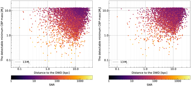
Figure 5: The relationship between the distance and the detectable minimum CBP mass for Taiji (left) and LISA (right) for promising systems in MLDC Round 4 during a nominal 4-year mission. The color represents the SNR of each system, and the dashed horizontal grey line corresponds to the deuterium burning limit.

4.2.2 Constraints on the promising systems in our Galaxy

We mentioned in Sec. 3.1 that $\mathrm{SNR}>10$ is chosen to be the threshold for our work, and in MLDC Round 4 there are 25,016 (15,903) detached DWDs satisfying this criterion for Taiji (LISA). Based on these populations, we find a total of 9,053 (6,718) promising systems at most during a 4-year observation for Taiji (LISA). Figure 5 shows that most systems are clustered together in the 1–13 $M_{\mathrm{J}}$ mass range and at about 10 kpc from our Solar system, which is consistent with the distance to the Galactic center. Generally, nearby DWDs could have lower $M_{\mathrm{p}}^{\mathrm{min}}$ than distant systems due to their higher SNRs. This also explains why the promising systems are mainly distributed in the top right of Fig. 5.

To go a step further, we plot the distributions of the detectable minimum (maximum) period and corresponding IDZ (ODZ) in Fig. 6. We see that some valleys appear at multiples of one year, which correspond to the peaks in Fig. 3, caused by the degeneracies between source and detector parameters (see Sec. 4.1). From the bottom panels, we see that Taiji is expected to detect CBPs with the planetary orbital size smaller than 5 au, which is about the distance from the Sun to the Jupiter (5.2 au), while it is a little smaller (4.4 au) for LISA. The constraints on DZs actually reflect the detecting ability of the space-borne GW detector we choose, because these results are based on the population of DWDs without injecting any CBP models. It shows that the best range of detection is between 0.1 au to 3 au for both LISA and Taiji.

For each promising system, the dependence of IDZ and ODZ on the GW frequency are illustrated in Fig. 7. Our results seem to suggest that systems with higher GW frequencies tend to have wider DZs. An explanation for this may come from the higher SNRs in the sensitive frequency band, namely 0.1 mHz to 1 Hz for LISA and Taiji (see Sec. 2.1 and Fig. 2). Note that there are some gaps at distance $\lesssim 1$ au in Fig. 7, which is due to our sample intervals in the parameter estimation process and would not alter the qualitative conclusion derived here.

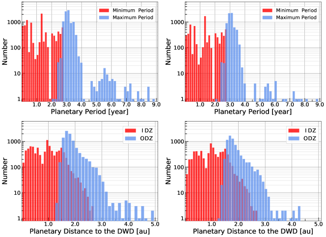
Figure 6: The distributions of detectable minimum and maximum period (top panels), and corresponding IDZ and ODZ (bottom panels). Left panels are for Taiji while right panels are for LISA.

4.2.3 Detection rates for different CBP models

As mentioned in Sec. 3.2, we only consider the coplanar orbits and the occurrence rate is set to 50% for the promising detectable systems. Based on the catalog of approximately $2.5\times 10^{4}$ ($1.6\times 10^{4}$) detectable detached DWDs for Taiji (LISA) in total (see Sec. 4.2.2), our model predicts that the total number of the injected CBP population is 4,507 (3,322) during the nominal mission span.

Following Danielski et al. (2019), we consider two scenarios in our sub-stellar object (SSO) injection processes:

1. an optimistic case where $a$ follows a log-uniform distribution in the range of $0.1$ – $200\,\mathrm{au}$, and $M_{\mathrm{p}}$ is uniformly distributed in the range of $1\,{M}_{\oplus}$ – $0.08\,{M_{\odot}}$, and

2. a pessimistic scenario where $a$ is uniformly distributed in the range of $0.1$ – $200\,\mathrm{au}$, and $M_{\mathrm{p}}$ is uniformly distributed in the range of $1\,{M}_{\oplus}$ – $0.08\,{M_{\odot}}$.

Note that samples with an injected SSO mass $13\,M_{\mathrm{J}}<M<0.08\,{M_{\odot}}$ are discarded because we only focus on the CBPs with mass $M_{\mathrm{p}}\leq 13\,M_{\mathrm{J}}$ in this work. More discussions on brown dwarfs with mass $13\,M_{\mathrm{J}}<M<0.08\,{M_{\odot}}$ can be found in Danielski et al. (2019)

We find a total of 40 (16) detected CBPs for (A), 2 (0) for (B), corresponding to 0.16% (0.10%) and 0.008% (0%) of the total population of detected DWDs over the 4-year mission of Taiji (LISA). From these we conclude that the detection rates in our work are essentially in agreement with the results in Danielski et al. (2019), but a little bit more pessimistic as a whole due to the different underlying models and assumptions. Therefore, it is advantageous to improve CBP models in future for more comparisons. Although there seems like no detection in scenario (B) for LISA, Taiji can still has a non-zero result on CBP detections. These data again suggest that Taiji has a better performance on detecting abilities.

4.2.4 Prospects for detections of CBPs in habitable zone around DWDs

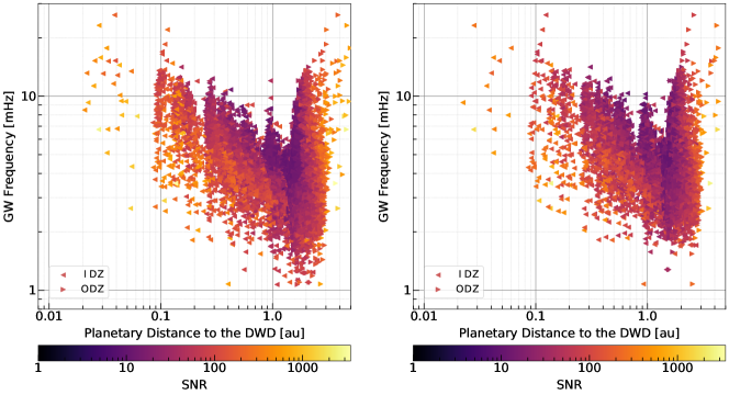
Figure 7: Dependence of IDZ and ODZ on the GW frequency of each promising system. The color represents the SNR of each system for Taiji (left) and LISA (right). We use the left and right triangles to denote the IDZ and ODZ respectively. Notice that for each system, its IDZ and ODZ are located in the same horizontal line (i.e. they have the same GW frequency).

The discovery of thousands of exoplanets in past decades has been promoting the study of habitability and the search for extraterrestrial life (Cockell et al., 2016; Kaltenegger, 2017; Lingam & Loeb, 2018), which encompass various research methods within the physical, biological, and environmental sciences. Among many contemporary habitability metrics, the habitable zone (HZ) forms a fundamental component to assess the potential habitability of newly discovered exoplanets. It describes the circumstellar distance where water at the surface of an exoplanet would be in the liquid phase (Kasting et al., 1993), mainly because all life on the Earth requires liquid water directly or indirectly. Given that the Earth is the only known planet with life on it, it is reasonable to suppose that such a concept also applies to exoplanets beyond the Earth.

Most research about HZ has focused on MS stars that are similar to the Sun (Kasting et al., 1993; Selsis et al., 2007; Lunine et al., 2008; Rushby et al., 2013). But recent studies start to discuss the HZ of WDs (Monteiro, 2010; Agol, 2011; Fossati et al., 2012; Barnes & Heller, 2013). Although, unlike hydrogen-burning stars, the WD cooling makes the HZ moves inwards with time, WDs are still expected to provide a source of energy for planets in HZ for giga-year (Gyr) durations. As the remnants of MS stars, WDs are as abundant as Sun-like stars in our Galaxy. Most of them are close in size to our Earth with a characteristic luminosity of $\sim 10^{-4}\,L_{\odot}$ (Agol, 2011). So the HZ around WDs is located within $\sim 0.01$ au where planets must have migrated inwards after the CE phases (Debes & Sigurdsson, 2002; Livio et al., 2005; Faedi et al., 2011). As noted by Tamanini & Danielski (2019), the detection of such an exoplanet would help to provide crucial information on migration theories, especially around post-CE binaries.

We assume that the HZ boundary estimations for MS stars also apply to DWD systems. Thus we can determine the inner/outer edge of the HZ (referred to as IHZ/OHZ) via equations in Selsis et al. (2007),

$$\begin{split}\mathrm{IHZ}&=(\mathrm{IHZ}_{\odot}-a_{\mathrm{in}}T_{\star}-b_{\mathrm{in}}T_{\star}^{2})\big{(}\frac{L}{L_{\odot}}\big{)}^{1/2}\,,\\ \mathrm{OHZ}&=(\mathrm{OHZ}_{\odot}-a_{\mathrm{out}}T_{\star}-b_{\mathrm{out}}T_{\star}^{2})\big{(}\frac{L}{L_{\odot}}\big{)}^{1/2}\,,\end{split}$$ (18)

where $\mathrm{IHZ}_{\odot}$ and $\mathrm{OHZ}_{\odot}$ are the boundaries in our Solar system depending on different fractional cloud cover on the day side of an exoplanet (see Table 2). As noted in the Sec. 2 of Selsis et al. (2007), clouds can increase the planetary albedo and reduce the greenhouse warming, which thus moves $\mathrm{IHZ}_{\odot}$ closer to the star. But for $\mathrm{OHZ}_{\odot}$ associated with $\mathrm{CO_{2}}$-ice clouds, which differ significantly from $\mathrm{H_{2}O}$-ice particles in the optical properties, the cooling effect caused by the increase of albedo is weaker than the warming effect caused by the backscattering of the infrared surface emission (Lunine et al., 2008). As a result, the theoretical $\mathrm{OHZ}_{\odot}$ should be farther for a 100% cloud cover. Other empirically determined constants in Eq. (18) are,

$$a_{\mathrm{in}} =2.7619\times 10^{-5}\,{\rm au\,K^{-1}}\,,$$

$$b_{\mathrm{in}} =3.8095\times 10^{-9}\,\mathrm{au\,K^{-2}}\,,$$

$$a_{\mathrm{out}} =1.3786\times 10^{-4}\,{\rm au\,K^{-1}}\,,$$

$$b_{\mathrm{out}} =1.4286\times 10^{-9}\,\mathrm{au\,K^{-2}}\,.$$ (19)

In Eq. (18), $L$ and $L_{\odot}$ are the primary’s and Solar luminosity, respectively, and $T_{\star}=T_{\mathrm{eff}}-5700$ K, where the effective temperature of the primary $T_{\mathrm{eff}}$ is given according to the Stefan-Boltzmann law via,

$$T_{\mathrm{eff}}=\left(\frac{L}{4\pi\sigma R^{2}}\right)^{1/4}\,,$$ (20)

with $\sigma$ being the Stefan-Boltzmann constant and $R$ being the primary’s radius.

Table 2: Detection numbers and percentages of habitable CBPs around the promising systems for LISA and Taiji. We have mentioned in Sec. 4.2.2 that the total number of promising systems is 9,053 for Taiji, and 6,718 for LISA for a 4-yr mission.

Clouds 0%

Clouds 50%

Clouds 100%

Detector

$\mathrm{IHZ}_{\odot}$

$\mathrm{OHZ}_{\odot}$

IHZ

OHZ

$\mathrm{IHZ}_{\odot}$

$\mathrm{OHZ}_{\odot}$

IHZ

OHZ

$\mathrm{IHZ}_{\odot}$

$\mathrm{OHZ}_{\odot}$

IHZ

OHZ

[au]

[au]

[au]

[au]

[au]

[au]

[au]

[au]

[au]

[au]

[au]

[au]

0.895

1.67

0.013

0.024

0.72

1.95

0.010

0.028

0.485

2.4

0.0069

0.034

Taiji

$3\quad(0.033\%)$

$5\quad(0.055\%)$

$13\quad(0.14\%)$

LISA

$1\quad(0.015\%)$

$1\quad(0.015\%)$

$3\quad(0.45\%)$

As noted by Barnes & Heller (2013), WDs cool rapidly for about 3 Gyr, and then maintain a relatively constant temperature before falling off again at about 7 Gyr. As a rough estimation, we neglect the distributions of cooling time and assume that each WD has the same fixed luminosity value for which we set it to $1\times 10^{-4}$ $L_{\odot}$, with a total luminosity $2\times 10^{-4}$ $L_{\odot}$. Through the mass-radius relation for WDs in the Newtonian case, as provided in Fig. 4 of Ambrosino (2020), we calculate $T_{\mathrm{eff}}$ of each promising system. Based on our assumption, the two WDs have the same mass in the DWD system, therefore their $T_{\mathrm{eff}}$ values are the same as well. We plug $T_{\mathrm{eff}}$ into Eq. (18) to obtain the IHZ and OHZ of each promising system. We verify that ODZ is much farther than OHZ for each system due to the low luminosities of WDs, which means that we only need to compare the limits between OHZ and IDZ. If the IDZ lies closer to the DWD than the OHZ, we can say that LISA and Taiji are possible to detect a habitable CBP around this system.

We list our results in Table 2 for LISA and Taiji during a 4-year observation. Note that for each cloud cover scheme, we take the same values of IHZ and OHZ as a criterion because the boundary values of HZ are insensitive to $T_{\mathrm{eff}}$ in our simplified model. Although the detection numbers do not seem many, it still shows that such a possibility exists. We also have verified that the detection number would not increase by more than one order of magnitude if we set the total luminosity to $2\times 10^{-3}\,L_{\odot}$, which is larger than what they really are when the WD cooling is considered (see e.g. Fig. 1 in Barnes & Heller, 2013).

5 Conclusion

In this work, we introduce the two space-borne GW detectors, LISA and Taiji, and discuss the use of them to detect exoplanets. For the GW detection method originally proposed by Tamanini & Danielski (2019), we give some complementary calculations on the detecting abilities with different values of binary mass and mass ratio. The conceptual idea using LISA/Taiji to detect exoplanets is similar to the RV technique but has unique advantages, compared to the traditional EM methods. Before quantitatively analyzing the prospects for detecting CBPs around DWDs in the whole Galaxy by using LISA and Taiji, we show that there is a possibility to detect CBPs around four known detached DWDs with high SNRs using Taiji, while three systems are also promising for LISA. The minimum detectable masses around these DWDs can be as small as a few of the Jupiter mass. Moreover, if EM observations can give more constraints on these systems in the meantime, e.g. inferring the orbital inclination of the CBP, GWs may place more restrictions on the mass of the CBP and the existence of such a population.

Based on the DWD population from MLDC Round 4, we give quick assessments of CBP detections in the whole Galaxy during a 4-yr mission time of LISA/Taiji. Our results show that LISA can detect $\sim 6,000$ promising systems, while the number rises to $\sim 9,000$ for Taiji. From the distributions of DZs, we show that the best range of CBP detections is between 0.1 au to 3 au around DWDs for both LISA and Taiji. Furthermore, we inject two different planet distributions with an occurrence rate of 50%, following Danielski et al. (2019), to constrain the total detection rates. Our results are in bold agreement with previous studies, but seem slightly more pessimistic as a whole due to the different models and assumptions we adopted. By assuming that the HZ boundary estimations for MS stars also apply to DWDs, we briefly discuss the prospects for detecting habitable CBPs around detached DWDs in a simplified model. It shows that such a possibility exists though the detection rates are not large during 4-yr observations.

In addition to the planetary migration theories (Turrini et al., 2015), there are also some studies about the second-generation formation process which can be used to explain the existence of nearby exoplanets in these systems (Zorotovic & Schreiber, 2013; Völschow et al., 2014; Schleicher & Dreizler, 2014). All our results can actually help analyze planetary systems after CE phases and provide a useful input for exoplanetary projects. With a rapid development of GW astronomy in the past 5 years, we look forward to the synergy with EM observations and the full investigation of such a GW detection method of exoplanets in the near future.

Table 3: Properties of the selected known detached DWDs (Huang et al., 2020). Some inclination angles are given with a square bracket due to lack of direct measurements of them. These estimated values are assigned based on the evolutionary stage and the mass ratio of the system. The asterisk marks a corrected distance from Burdge et al. (2019).

Source	$m_{1}$		$m_{2}$		$f$	$d_{\mathrm{DWD}}$	$\lambda$		$\beta$		$\iota$
	[$\mathrm{M_{\odot}}$]		[$\mathrm{M_{\odot}}$]		[mHz]	[kpc]	[deg]		[deg]		[deg]
ZTF J153932.16+502738.8	0.	61	0.	21	4.82	2.34*	205.	03	66.	16	84.	0
SDSS J065133.34+284423.4	0.	49	0.	247	2.61	0.933	101.	34	5.	80	86.	9
SDSS J093506.92+441107.0	0.	75	0.	312	1.68	0.645	130.	98	28.	09	[60.	0]
SDSS J232230.20+050942.06	0.	27	0.	24	1.66	0.779	353.	44	8.	46	27.	0
PTF J053332.05+020911.6	0.	65	0.	167	1.62	1.253	82.	91	$-21$.	12	72.	8
SDSS J163030.58+423305.7	0.	76	0.	298	0.84	1.019	231.	76	63.	05	[60.	0]
SDSS J092345.59+302805.0	0.	76	0.	275	0.51	0.299	133.	72	14.	43	[60.	0]

References

- Abbott et al. (2016) Abbott, B. P., et al. 2016, PhRvL, 116, 061102, doi: 10.1103/PhysRevLett.116.061102
- Abbott et al. (2017) —. 2017, PhRvL, 119, 161101, doi: 10.1103/PhysRevLett.119.161101
- Agol (2011) Agol, E. 2011, ApJL, 731, L31, doi: 10.1088/2041-8205/731/2/L31
- Althaus et al. (2010) Althaus, L. G., Corsico, A. H., Isern, J., & a Berro, E. G. 2010, A&ARv, 18, 471, doi: 10.1007/s00159-010-0033-1
- Amaro-Seoane et al. (2017) Amaro-Seoane, P., et al. 2017. https://arxiv.org/abs/1702.00786
- Ambrosino (2020) Ambrosino, F. 2020. https://arxiv.org/abs/2012.01242
- Babak et al. (2008) Babak, S., et al. 2008, CQGra, 25, 184026, doi: 10.1088/0264-9381/25/18/184026
- Babak et al. (2010) —. 2010, CQGra, 27, 084009, doi: 10.1088/0264-9381/27/8/084009
- Barnes & Heller (2013) Barnes, R., & Heller, R. 2013, AsBio, 13, 279, doi: 10.1089/ast.2012.0867
- Berti et al. (2005) Berti, E., Buonanno, A., & Will, C. M. 2005, PhRvD, 71, 084025, doi: 10.1103/PhysRevD.71.084025
- Beuermann et al. (2010) Beuermann, K., et al. 2010, A&A, 521, L60, doi: 10.1051/0004-6361/201015472
- Beuermann et al. (2011) —. 2011, A&A, 526, A53, doi: 10.1051/0004-6361/201015942
- Breivik et al. (2020) Breivik, K., et al. 2020, ApJ, 898, 71, doi: 10.3847/1538-4357/ab9d85
- Brown et al. (2017) Brown, J. C., Veras, D., & Gänsicke, B. T. 2017, MNRAS, 468, 1575, doi: 10.1093/mnras/stx428
- Brown et al. (2020) Brown, W. R., Kilic, M., Kosakowski, A., et al. 2020, ApJ, 889, 49, doi: 10.3847/1538-4357/ab63cd
- Burdge et al. (2019) Burdge, K. B., et al. 2019, Natur, 571, 528, doi: 10.1038/s41586-019-1403-0
- Cockell et al. (2016) Cockell, C. S., Bush, T., Bryce, C., et al. 2016, AsBio, 16, 89, doi: 10.1089/ast.2015.1295
- Cornish & Larson (2003) Cornish, N. J., & Larson, S. L. 2003, PhRvD, 67, 103001, doi: 10.1103/PhysRevD.67.103001
- Cutler (1998) Cutler, C. 1998, Phys. Rev. D, 57, 7089, doi: 10.1103/PhysRevD.57.7089
- Cutler & Thorne (2002) Cutler, C., & Thorne, K. S. 2002, in General Relativity and Gravitation, ed. N. T. Bishop & S. D. Maharaj, 72–111, doi: 10.1142/9789812776556_0004
- Danielski et al. (2019) Danielski, C., Korol, V., Tamanini, N., & Rossi, E. M. 2019, A&A, 632, A113, doi: 10.1051/0004-6361/201936729
- Danielski & Tamanini (2020) Danielski, C., & Tamanini, N. 2020, IJMPD, 29, 2043007, doi: 10.1142/S0218271820430075
- Debes & Sigurdsson (2002) Debes, J. H., & Sigurdsson, S. 2002, ApJ, 572, 556, doi: 10.1086/340291
- Duchêne & Kraus (2013) Duchêne, G., & Kraus, A. 2013, ARA&A, 51, 269, doi: 10.1146/annurev-astro-081710-102602
- Duncan & Lissauer (1998) Duncan, M. J., & Lissauer, J. J. 1998, Icar, 134, 303, doi: 10.1006/icar.1998.5962
- Dvorak (1986) Dvorak, R. 1986, A&A, 167, 379
- Eberle et al. (2008) Eberle, J., Cuntz, M., & Musielak, Z. E. 2008, A&A, 489, 1329, doi: 10.1051/0004-6361:200809758
- Faedi et al. (2011) Faedi, F., West, R. G., Burleigh, M. R., Goad, M. R., & Hebb, L. 2011, MNRAS, 410, 899, doi: 10.1111/j.1365-2966.2010.17488.x
- Farihi (2016) Farihi, J. 2016, New A Rev., 71, 9, doi: 10.1016/j.newar.2016.03.001
- Farihi et al. (2018) Farihi, J., van Lieshout, R., Cauley, P. W., et al. 2018, MNRAS, 481, 2601, doi: 10.1093/mnras/sty2331
- Fossati et al. (2012) Fossati, L., Bagnulo, S., Haswell, C. A., et al. 2012, ApJL, 757, L15, doi: 10.1088/2041-8205/757/1/L15
- Foucart & Lai (2013) Foucart, F., & Lai, D. 2013, ApJ, 764, 106, doi: 10.1088/0004-637X/764/1/106
- Holman & Wiegert (1999) Holman, M. J., & Wiegert, P. A. 1999, AJ, 117, 621, doi: 10.1086/300695
- Hong & van Putten (2021) Hong, C., & van Putten, M. H. P. M. 2021, New A, 84, 101516, doi: 10.1016/j.newast.2020.101516
- Huang et al. (2020) Huang, S.-J., Hu, Y.-M., Korol, V., et al. 2020, PhRvD, 102, 063021, doi: 10.1103/PhysRevD.102.063021
- Jura et al. (2009) Jura, M., Farihi, J., & Zuckerman, B. 2009, AJ, 137, 3191, doi: 10.1088/0004-6256/137/2/3191
- Kaltenegger (2017) Kaltenegger, L. 2017, ARA&A, 55, 433, doi: 10.1146/annurev-astro-082214-122238
- Kasting et al. (1993) Kasting, J. F., Whitmire, D. P., & Reynolds, R. T. 1993, Icar, 101, 108, doi: 10.1006/icar.1993.1010
- Kennedy et al. (2012) Kennedy, G. M., Wyatt, M. C., Sibthorpe, B., et al. 2012, MNRAS, 426, 2115, doi: 10.1111/j.1365-2966.2012.21865.x
- Klein et al. (2016) Klein, A., Barausse, E., Sesana, A., et al. 2016, Phys. Rev. D, 93, 024003, doi: 10.1103/PhysRevD.93.024003
- Koester et al. (2014) Koester, D., Gänsicke, B. T., & Farihi, J. 2014, A&A, 566, A34, doi: 10.1051/0004-6361/201423691
- Korol et al. (2018) Korol, V., Koop, O., & Rossi, E. M. 2018, ApJL, 866, L20, doi: 10.3847/2041-8213/aae587
- Korol et al. (2017) Korol, V., Rossi, E. M., Groot, P. J., et al. 2017, MNRAS, 470, 1894, doi: 10.1093/mnras/stx1285
- Korol et al. (2020) Korol, V., et al. 2020, A&A, 638, A153, doi: 10.1051/0004-6361/202037764
- Lamberts et al. (2019) Lamberts, A., Blunt, S., Littenberg, T. B., et al. 2019, MNRAS, 490, 5888, doi: 10.1093/mnras/stz2834
- Lamberts et al. (2018) Lamberts, A., Garrison-Kimmel, S., Hopkins, P., et al. 2018, MNRAS, 480, 2704, doi: 10.1093/mnras/sty2035
- Lingam & Loeb (2018) Lingam, M., & Loeb, A. 2018, JCAP, 05, 020, doi: 10.1088/1475-7516/2018/05/020
- Livio et al. (2005) Livio, M., Pringle, J. E., & Wood, K. 2005, ApJL, 632, L37, doi: 10.1086/497577
- Livio & Soker (1984) Livio, M., & Soker, N. 1984, MNRAS, 208, 763, doi: 10.1093/mnras/208.4.763
- Lunine et al. (2008) Lunine, J. I., et al. 2008. https://arxiv.org/abs/0808.2754
- Luo et al. (2020) Luo, Z., Guo, Z., Jin, G., Wu, Y., & Hu, W. 2020, ResPh, 16, 102918, doi: 10.1016/j.rinp.2019.102918
- Monteiro (2010) Monteiro, H. 2010, BASBr, 29, 22
- Mustill et al. (2018) Mustill, A. J., Villaver, E., Veras, D., Gänsicke, B. T., & Bonsor, A. 2018, MNRAS, 476, 3939, doi: 10.1093/mnras/sty446
- Nelemans & Tauris (1998) Nelemans, G., & Tauris, T. M. 1998, A&A, 335, L85. https://arxiv.org/abs/astro-ph/9806011
- Nelemans et al. (2001) Nelemans, G., Yungelson, L. R., & Portegies Zwart, S. F. 2001, A&A, 375, 890, doi: 10.1051/0004-6361:20010683
- Raghavan et al. (2010) Raghavan, D., McAlister, H. A., Henry, T. J., et al. 2010, ApJS, 190, 1, doi: 10.1088/0067-0049/190/1/1
- Ramsay et al. (2018) Ramsay, G., Green, M. J., Marsh, T. R., et al. 2018, A&A, 620, A141, doi: 10.1051/0004-6361/201834261
- Robson et al. (2019) Robson, T., Cornish, N. J., & Liu, C. 2019, CQGra, 36, 105011, doi: 10.1088/1361-6382/ab1101
- Roebber et al. (2020) Roebber, E., et al. 2020, ApJL, 894, L15, doi: 10.3847/2041-8213/ab8ac9
- Ruan et al. (2020) Ruan, W.-H., Liu, C., Guo, Z.-K., Wu, Y.-L., & Cai, R.-G. 2020, NatAs, 4, 108, doi: 10.1038/s41550-019-1008-4
- Rushby et al. (2013) Rushby, A. J., Claire, M. W., Osborn, H., & Watson, A. J. 2013, AsBio, 13, 833, doi: 10.1089/ast.2012.0938
- Schleicher & Dreizler (2014) Schleicher, D. R. G., & Dreizler, S. 2014, A&A, 563, A61, doi: 10.1051/0004-6361/201322860
- Selsis et al. (2007) Selsis, F., Kasting, J. F., Levrard, B., et al. 2007, A&A, 476, 1373, doi: 10.1051/0004-6361:20078091
- Seto (2008) Seto, N. 2008, Astrophys. J. Lett., 677, L55, doi: 10.1086/587785
- Shi et al. (2019) Shi, C., Bao, J., Wang, H.-T., et al. 2019, Phys. Rev. D, 100, 044036, doi: 10.1103/PhysRevD.100.044036
- Sigurdsson (1993) Sigurdsson, S. 1993, ApJ, 415, L43, doi: 10.1086/187028
- Smallwood et al. (2018) Smallwood, J. L., Martin, R. G., Livio, M., & Lubow, S. H. 2018, MNRAS, 480, 57, doi: 10.1093/mnras/sty1819
- Takahashi & Seto (2002) Takahashi, R., & Seto, N. 2002, ApJ, 575, 1030, doi: 10.1086/341483
- Tamanini & Danielski (2019) Tamanini, N., & Danielski, C. 2019, NatAs, 3, 858, doi: 10.1038/s41550-019-0807-y
- Thorsett et al. (1993) Thorsett, S. E., Arzoumanian, Z., & Taylor, J. H. 1993, ApJ, 412, L33, doi: 10.1086/186933
- Turrini et al. (2015) Turrini, D., Nelson, R. P., & Barbieri, M. 2015, ExA, 40, 501, doi: 10.1007/s10686-014-9401-6
- Veras (2016) Veras, D. 2016, RSOS, 3, 150571, doi: 10.1098/rsos.150571
- Veras & Tout (2012) Veras, D., & Tout, C. A. 2012, MNRAS, 422, 1648, doi: 10.1111/j.1365-2966.2012.20741.x
- Veras et al. (2011) Veras, D., Wyatt, M. C., Mustill, A. J., Bonsor, A., & Eldridge, J. J. 2011, MNRAS, 417, 2104, doi: 10.1111/j.1365-2966.2011.19393.x
- Völschow et al. (2014) Völschow, M., Banerjee, R., & Hessman, F. V. 2014, A&A, 562, A19, doi: 10.1051/0004-6361/201322111
- Wang & Han (2021) Wang, G., & Han, W.-B. 2021, PhRvD, 103, 064021, doi: 10.1103/PhysRevD.103.064021
- Wong et al. (2019) Wong, K. W. K., Berti, E., Gabella, W. E., & Holley-Bockelmann, K. 2019, MNRAS, 483, L33, doi: 10.1093/mnrasl/sly208
- Yu & Jeffery (2010) Yu, S., & Jeffery, C. S. 2010, A&A, 521, A85, doi: 10.1051/0004-6361/201014827
- Zorotovic & Schreiber (2013) Zorotovic, M., & Schreiber, M. R. 2013, A&A, 549, A95, doi: 10.1051/0004-6361/201220321