Comparison of planetary H $\alpha$-emission models: A new correlation with accretion luminosity

Abstract

Accreting planets have been detected through their hydrogen-line emission, specifically H $\alpha$. To interpret this, stellar-regime empirical correlations between the H $\alpha$ luminosity $L_{\mathrm{H\,\alpha}}$ and the accretion luminosity $L_{\mathrm{acc}}$ or accretion rate $\dot{M}$ have been extrapolated to planetary masses, however without validation. We present a theoretical $L_{\mathrm{acc}}$–$L_{\mathrm{H\,\alpha}}$ relationship applicable to a shock at the surface of a planet. We consider wide ranges of accretion rates and masses and use detailed spectrally-resolved, non-equilibrium models of the postshock cooling. The new relationship gives a markedly higher $L_{\mathrm{acc}}$ for a given $L_{\mathrm{H\,\alpha}}$ than fits to young stellar objects, because Ly $\alpha$, which is not observable, carries a large fraction of $L_{\mathrm{acc}}$. Specifically, an $L_{\mathrm{H\,\alpha}}$ measurement needs ten to 100 times higher $L_{\mathrm{acc}}$ and $\dot{M}$ than previously predicted, which may explain the rarity of planetary H $\alpha$ detections. We also compare the $\dot{M}$–$L_{\mathrm{H\,\alpha}}$ relationships coming from the planet-surface shock or implied by accretion-funnel emission. Both can contribute simultaneously to an observed H $\alpha$ signal but at low (high) $\dot{M}$ the planetary-surface shock (heated funnel) dominates. Only the shock produces Gaussian line wings. Finally, we discuss accretion contexts in which different emission scenarios may apply, putting recent literature models in perspective, and also present $L_{\mathrm{acc}}$–$L_{\mathrm{line}}$ relationships for several other hydrogen lines.

1 Introduction

Recent observations have detected H $\alpha$ emission from planets around young accreting stars (Wagner et al., 2018; Haffert et al., 2019, hereafter H19; Hashimoto et al., 2020; Eriksson et al., 2020). For stars, sufficiently strong H $\alpha$ indicates gas accretion (Hartmann et al., 2016), and empirical relationships between H $\alpha$ luminosity and accretion luminosity exist, where the latter is estimated from UV continuum observations (e.g., Fang et al., 2009). Because initially no $L_{\mathrm{H}\,\alpha}$–$L_{\mathrm{acc}}$ correlations were available for the planetary case, these stellar scalings have been extrapolated to analyse individual detections or surveys results (Sallum et al., 2015; Wagner et al., 2018; H19; Cugno et al., 2019; Zurlo et al., 2020; Xie et al., 2020). However, verifying whether these correlations hold also at planetary masses was not yet possible.

Following the reports on planetary H $\alpha$ detection, theoretical work has attempted to reproduce and interpret the observations. Thanathibodee et al. (2019, hereafter Th19) applied a magnetospheric accretion model developed for T Tauri stars (Muzerolle et al., 2001) to planetary masses and radii, and could reproduce the H $\alpha$ line of PDS 70 b. They assumed a strong magnetic field able to truncate the accretion disc (Christensen et al., 2009; Batygin, 2018) and hot gas ($T\sim 10^{4}$ K) in the accretion funnel.

In another direction, Aoyama et al. (2018, hereafter AIT18) constructed the first emission model of shock-heated gas for planetary masses, focusing on hydrogen lines. There, the H $\alpha$ comes from the postshock gas and not the accretion flow. This can reproduce the observations if a strong shock of preshock velocity $v\gtrsim 30~{}\mathrm{km}\,\mathrm{s^{-1}}$ occurs on the circumplanetary disc (CPD) surface or on the planetary surface (Aoyama & Ikoma, 2019, hereafter AI19). The former is suggested by isothermal 3D hydrodynamic simulations (Tanigawa et al., 2012), in which the gas flows almost vertically in free-fall onto the CPD. A planetary-surface shock can occur when the gas falls directly from the upper layers of the protoplanetary disc (PPD), for instance, from meridional circulation (Szulágyi et al., 2014; Teague et al., 2019) or through magnetospheric accretion columns originating at the inner edge of the CPD (e.g., Lovelace et al., 2011; Batygin, 2018). Such flow patterns need non-isothermal or magnetic effects, respectively.

In this Letter, we derive new theoretical $L_{\mathrm{acc}}$–$L_{\mathrm{H}\,\alpha}$ and $\dot{M}$–$L_{\mathrm{H}\,\alpha}$ relationships from our shock emission model for planetary-surface accretion. We compare them with correlations measured for stars. Afterward, we discuss the differences among theoretical models and predictions, including Szulágyi & Ercolano (2020, hereafter SzE20). We also comment in Appendix B on the $L_{\mathrm{H}\,\alpha}$ estimate by Zhu (2015), and present correlations for several other lines in Appendix C.

2 Stellar and planetary accretion relationships

2.1 Comparison of $L_{\mathrm{acc}}$–$L_{\mathrm{H}\,\alpha}$ relationships

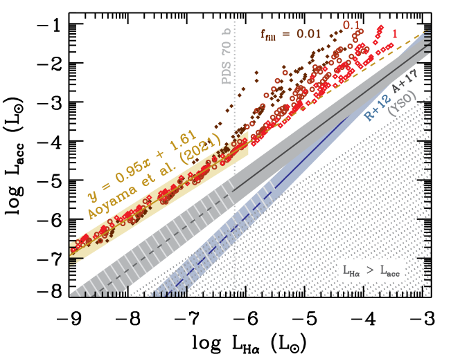
Figure 1: Theoretical relationships between accretion luminosity, $L_{\mathrm{acc}}$ and H $\alpha$ luminosity, $L_{\mathrm{H}\,\alpha}$. The symbols show our model results for a wide range of accretion rates $\dot{M}=3\times 10^{-10}$–$3\times 10^{-5}~{}M_{\mathrm{J}}/\mathrm{yr}$ and masses $M_{\mathrm{p}}=2$–20 $M_{\mathrm{J}}$, with filling factor $f_{\mathrm{fill}}=0.01$ (filled diamonds), $0.1$ (circles), and $1$ (open diamonds). The golden line indicates Equation (1) which fits our results up to $\log(L_{\mathrm{acc}}/L_{\odot})=-4$; the dashed line is an extrapolation. The shaded golden region shows the spread $\pm\sigma=\pm 0.3$ dex. Fits by Rigliaco et al. (2012, blue) and Alcalá et al. (2017, gray) for stellar-mass objects are also shown by the blue and gray lines, respectively. The shaded regions reflect the formal errors (Equation (A1), with $\sigma_{\log L_{\mathrm{H}\,\alpha}}=0$), which corresponds to the usual approach but ignores the spread of their data ($\pm\sigma\approx\pm 0.5$–0.7 dex). The dashed lines indicate extrapolations. Extinction by material around the planet (not included) would only move the points to the left, away from the stellar relationships. Already without considering extinction, our relationship differs clearly from the stellar fits, by up to 2.5 dex here. The dotted region has $L_{\mathrm{H}\,\alpha}>L_{\mathrm{acc}}$, which could be unlikely (see text).

In stellar observations, UV/optical continuum measurements (e.g., Gullbring et al., 1998) have been used to estimate the accretion luminosity $L_{\mathrm{acc}}$ by modeling the emission from the shock-heated photosphere (e.g., Calvet & Gullbring, 1998). However, for distant objects, interstellar extinction prevents the detection of such continua. On the other hand, H $\alpha$ is brighter and less extincted. Thus, empirical $L_{\mathrm{acc}}$–$L_{\mathrm{H}\,\alpha}$ relationships derived for nearby stars are used to estimate $L_{\mathrm{acc}}$ from the observed $L_{\mathrm{H}\,\alpha}$. Then, assuming a mass and radius or using known estimates from photometry, $\dot{M}$ is estimated for distant accretors.

In Figure 1, we show the $L_{\mathrm{acc}}$–$L_{\mathrm{H}\,\alpha}$ correlation from AI19’s models, detailed in Aoyama et al. (2020, hereafter AMMI21). They simulated the radiative transfer of hydrogen lines in the 1D plane-parallel flow of the shock-heated gas. Since the timescale of temperature change is comparable to that of line emission process, they numerically calculated the time-evolving electron transitions via collision and radiation. This model estimates the hydrogen line intensity for two input parameters of pre-shock gas velocity $v_{0}$ and number density $n_{0}$. Assuming the accreting gas falls onto the planetary surface with the free-fall velocity, the model estimates the hydrogen line luminosity as a function of the planetary mass $M_{\mathrm{p}}$ and the accretion rate $\dot{M}$. As in AMMI21, $L_{\mathrm{acc}}=GM_{\mathrm{p}}\dot{M}(R_{\mathrm{p}}^{-1}-R_{\mathrm{in}}^{-1})$, where $G$ is the gravitational constant, $R_{\mathrm{p}}$ is the planetary radius and $R_{\mathrm{in}}$ is the radius from which the gas starts at rest. We consider a wide range of mass accretion rates $\dot{M}=3\times 10^{-10}$–$3\times 10^{-5}~{}M_{\mathrm{J}}/\mathrm{yr}$ and masses $M_{\mathrm{p}}=2$–20 $M_{\mathrm{J}}$, and consider a filling factor $f_{\mathrm{fill}}=0.01$, $0.1$, or $1$, where the H $\alpha$ emission comes from the area of the shock of $f_{\mathrm{fill}}4\pi R_{\mathrm{p}}^{2}$. For $f_{\mathrm{fill}}=1$, $R_{\mathrm{in}}=\infty$ (since $R_{\mathrm{in}}\approx 1/4R_{\mathrm{Hill}}\gg R_{\mathrm{p}}$, where $R_{\mathrm{Hill}}$ is the Hill radius; Mordasini et al., 2012), and $R_{\mathrm{in}}=5R_{\mathrm{p}}$ for $f_{\mathrm{fill}}\leqslant 0.1$ as for magnetospheric accretion (Hartmann et al., 2016). We use fits by AMMI21 of $R_{\mathrm{p}}(\dot{M},M_{\mathrm{p}})$ from the Mordasini et al. (2012) planet-structure model, which predicts $R_{\mathrm{p}}\approx 1.5$–5 $R_{\mathrm{J}}$.

For $L_{\mathrm{acc}}\lesssim 10^{-4}~{}L_{\odot}$, $L_{\mathrm{acc}}$ and $L_{\mathrm{H}\,\alpha}$ correlate well with each other. The spread in $L_{\mathrm{acc}}$ ($\lesssim 1.5$ dex) at higher $L_{\mathrm{acc}}$ reflects the large optical depth at H $\alpha$. In high-$L_{\mathrm{acc}}$ (or higher-density) cases, H $\alpha$ from optically thick regions hardly escapes, and other lines take over the energy transfer. Decreasing $f_{\mathrm{fill}}$ increases the (pre- and) postshock density and thus the postshock optical thickness (AIT18). Thus, decreasing $f_{\mathrm{fill}}$ also increases $L_{\mathrm{acc}}$ at a given $L_{\mathrm{H}\,\alpha}$, and $f_{\mathrm{fill}}=1$ yields the minimal $L_{\mathrm{acc}}$ for a given $L_{\mathrm{H}\,\alpha}$. Also, lower masses sit towards higher $L_{\mathrm{acc}}$ for a given $L_{\mathrm{H}\,\alpha}$ because $v_{0}$ is lower, causing a lower excitation degree and less effective hydrogen line emission.

We fit our $L_{\mathrm{acc}}$–$L_{\mathrm{H}\,\alpha}$ relationship in the form of $y=ax+b$ for $L_{\mathrm{acc}}\leqslant 10^{-4}~{}L_{\odot}$:

$$\log_{10}\left(L_{\mathrm{acc}}/L_{\odot}\right)=0.95\times\log_{10}\left(L_{\mathrm{H}\,\alpha}/L_{\odot}\right)+1.61,$$ (1)

where $L_{\odot}=3.84\times 10^{26}$ erg s^-1. The upward spread due to high optical depths barely affects the fit because optically thin cases are much more frequent for a uniform sampling of $M_{\mathrm{p}}$ and $\dot{M}$. The formal errorbars are $\sigma_{a}=0.006$ and $\sigma_{b}=0.04$, with the root-mean square residual $\mathrm{rms}=0.11$ dex, but the half-spread at a given $L_{\mathrm{H}\,\alpha}$ is $\sigma\approx 0.3$ dex (shaded region in Figure 1). We recommend using $\sigma=0.30$ as the uncertainty when determining $L_{\mathrm{acc}}$ from $L_{\mathrm{H}\,\alpha}$ and propagating errors (Appendix A).

We compare our fit to two empirical relationships derived for stars. The blue region in Figure 1 shows the relationship of Rigliaco et al. (2012, hereafter R12). To explain a given $L_{\mathrm{H}\,\alpha}$, R12’s fit requires an $L_{\mathrm{acc}}$ smaller than our estimate by up to two orders of magnitude. Since, in the shock model, the accretion energy is partitioned into the Ly $\alpha$ emission more by a factor of several tens than into the H $\alpha$ emission, such a high $L_{\mathrm{H}\,\alpha}/L_{\mathrm{acc}}$ ratio cannot be achieved. In contrast, in the magnetospheric accretion model used for interpreting the H $\alpha$ emission in the stellar regime, Ly $\alpha$ emission should be less efficient than in the planetary shock model due to, for example, large optical thickness. Also, we note that a part of stellar H $\alpha$ energy (i.e., the energy heating the accretion column) might come from the stellar interior energy through the magnetic field, in addition to the accretion energy. R12’s fit also differs greatly in slope from ours. This is because R12’s empirical relationship was derived using stellar objects of higher $\dot{M}$ (or $L_{\mathrm{acc}}$) than studied here; for more massive stars, more energy is emitted in the UV continuum rather than in optical lines such as H $\alpha$ (Zhou et al., 2014). This is also the reason why the $L_{\mathrm{acc}}$ estimated in Zhou et al. (2021) via UV continuum is lower than ours. For stellar cases with stronger shock, Ly $\alpha$ should be much weaker than UV continuum and negligible, and $L_{\mathrm{acc}}$ is well estimated only via UV continuum. But in the planetary shock emission, Ly $\alpha$ carries a large fraction of the energy, while this line is not observable due to strong circumstellar extinction. Even at TW Hya, one of the closest young stellar objects, the interstellar hydrogen column density is $\approx 10^{19.5}$ cm^-2 (Herczeg et al., 2004). Combined with the narrowness of the planetary Ly $\alpha$ line for low planet masses (full width at half maximum $\sim 0.3$ Å), this lets at most a percent of the Ly $\alpha$ reach us (Landsman & Simon, 1993). Thus, the flux ratio of Ly $\alpha$ to H $\alpha$ is around 0.1 or likely less, even at such a favourable target. For an object of $\gtrsim 20$ MJ, roughly ten times more Ly $\alpha$ passes through the ISM due to the greater line width.

Also, for $L_{\mathrm{H}\,\alpha}\lesssim 10^{-6}~{}L_{\odot}$, R12’s extrapolated fit suggests $L_{\mathrm{H}\,\alpha}>L_{\mathrm{acc}}$: more energy is emitted in H $\alpha$ than is brought in by the accreting gas. This is not necessarily unphysical, since the H $\alpha$ does not have to originate from the accretion shock, but seems unlikely since here the only other energy source is the interior luminosity (usually smaller than $L_{\mathrm{acc}}$; Mordasini et al., 2017).

The gray band in Figure 1 is from Alcalá et al. (2017, hereafter Al17), who extended the sample of Alcalá et al. (2014). Since Al17 fit only to very-low-mass stars, their slope should apply to planets presumably better more than R12. However, also Al17’s fitted line differs from ours by an order of magnitude. This reflects the contrasting H $\alpha$ emission mechanisms. Our model calculates H $\alpha$ from the shock-heated gas, while the stellar H $\alpha$ is thought to come (mainly) from an accretion funnel (Hartmann et al., 2016). Section 3.1 discusses this more extensively.

Our $L_{\mathrm{acc}}$–$L_{\mathrm{H}\,\alpha}$ relationship yields a higher $L_{\mathrm{acc}}$, for an observed $L_{\mathrm{H}\,\alpha}$, than both Al17, $y=1.13x+1.74$, and shallower R12, $y=1.49x+2.99$ do. Our curve also lies above those stellar correlations. Therefore, a measurement of (or upper limit on) $L_{\mathrm{H}\,\alpha}$ corresponds to a much higher accretion luminosity than inferred from the stellar fits. Since $\dot{M}$ is unknown within several orders of magnitude, whereas the mass and radius uncertainties are much smaller, $L_{\mathrm{acc}}$ should be set mostly by $\dot{M}$. Thus, an observed $L_{\mathrm{H}\,\alpha}$ corresponds to a higher $\dot{M}$ than inferred previously, suggesting that only strong accretors produce H $\alpha$ bright enough for detection. This might help explain the low yields of recent H $\alpha$ surveys (Cugno et al., 2019; Zurlo et al., 2020; Xie et al., 2020).

In Figure 1, a range of $L_{\mathrm{H}\,\alpha}$ values is covered both by the Al17 data and our model points (especially for $f_{\mathrm{fill}}\gtrsim 0.1$), at $L_{\mathrm{H}\,\alpha}\gtrsim 5\times 10^{-7}~{}L_{\odot}$. The two are separated by 1–2.5 dex at a given $L_{\mathrm{H}\,\alpha}$. However, the emission mechanisms likely differ (Section 3). Therefore, the two relationships need not match. Also, if at a given $L_{\mathrm{acc}}$ there are contributions from the shock and the accretion column, the latter probably dominates at high $\dot{M}$ (Section 2.2). If however the temperature in the accretion column is below $T\approx 10^{4}$ K or $\dot{M}$ is low, the surface shock more likely dominates.

Figure 1 shows the observed $L_{\mathrm{H}\,\alpha}$ value of PDS 70 b (vertical dotted line; Zhou et al., 2021) as a typical planetary $L_{\mathrm{H}\,\alpha}$ (cf. PDS 70 c and Delorme 1 (AB)b; Haffert et al., 2019; Eriksson et al., 2020). Our fit implies $L_{\mathrm{acc}}\approx 5\times 10^{-5}~{}L_{\odot}$, which is respectively about ten and 100 times larger than for Al17 and R12, with the latter in the $L_{\mathrm{H}\,\alpha}>L_{\mathrm{acc}}$ region. Our predicted $L_{\mathrm{acc}}$ is a lower limit if, as Hashimoto et al. (2020) infer, there is extinction.

2.2 Comparison of $\dot{M}$–$L_{\mathrm{H}\,\alpha}$ relationships

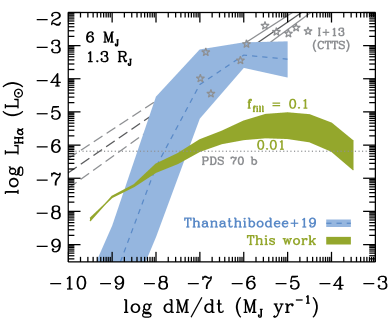
Figure 2: Restricted comparison of the $\dot{M}$–$L_{\mathrm{H}\,\alpha}$ relations for fixed $M_{\mathrm{p}}=6~{}M_{\mathrm{J}}$ and $R_{\mathrm{p}}=1.3~{}R_{\mathrm{J}}$ (only here) from Thanathibodee et al. (2019, blue band: 1 $\sigma$) and this work (green band). The bottom (top) border of our region is for $f_{\mathrm{fill}}=0.01$ (0.1), with Th19 finding $f_{\mathrm{fill}}=0.01$–0.1. Gray stars and lines show the Ingleby et al. (2013) data and fit ($\pm\sigma$) for CTTSs ($M\approx M_{\odot}$) for comparison. PDS 70 b is highlighted (gray dotted line; Zhou et al., 2021). For a version of this figure with extinction, see Marleau et al. (subm.).

A common approach in the literature is to use empirical $\dot{M}$–$L_{\mathrm{H}\,\alpha}$ correlations to infer $\dot{M}$. This approach hides the possibly complex dependence of $L_{\mathrm{H}\,\alpha}$ on several parameters into a best-fitting coefficient. Nevertheless, it is useful because $\dot{M}$ can vary by several orders of magnitude between objects while $M_{\mathrm{p}}/R_{\mathrm{p}}$ by much less, with $L_{\mathrm{H}\,\alpha}$ correlating with $L_{\mathrm{acc}}\propto M_{\mathrm{p}}\dot{M}/R_{\mathrm{p}}$ roughly.

We present in Figure 2 our $\dot{M}$–$L_{\mathrm{H}\,\alpha}$ relationship. To compare to Th19, we fix $M_{\mathrm{p}}=6~{}M_{\mathrm{J}}$ and $R_{\mathrm{p}}=1.3~{}R_{\mathrm{J}}$. Since Th19 assume magnetospheric accretion, we take $f_{\mathrm{fill}}=0.1$ and 0.01. Figure 2 shows that the dependence of $L_{\mathrm{H}\,\alpha}$ on $\dot{M}$ differs greatly between the surface shock (this work) and the heated accretion column (Th19). The latter has some overlap with the Classical T Tauri Stars (CTTSs) relationship of Ingleby et al. (2013), who fitted higher-mass objects than R12. Both in Th19 and here no extinction is considered. In our shock model, the emitted $L_{\mathrm{H}\,\alpha}$ less steeply depends on the $\dot{M}$ relative to the model of Th19.

The key point of Figure 2 is that the emission from the heated accretion column and that from the surface shock dominate in different regimes. Below a crossover value $\dot{M}_{\mathrm{cross}}$, the surface shock yields most of the H $\alpha$ luminosity, whereas at $\dot{M}\gtrsim\dot{M}_{\mathrm{cross}}$ the accretion column dominates. The Th19 models were fitted to a specific observation of a single object, and we too considered only one $(M_{\mathrm{p}},R_{\mathrm{p}})$ combination here. While $\dot{M}_{\mathrm{cross}}$ presumably depends on these parameters, the qualitative result that there is an $\dot{M}_{\mathrm{cross}}$ should be general.

If planets accrete mostly at $\dot{M}>\dot{M}_{\mathrm{cross}}$, the surface shock will not dominate $L_{\mathrm{H}\,\alpha}$. However, it is unclear how high $\dot{M}/\dot{M}_{\mathrm{cross}}$ can be. For PDS 70 b, Th19 fit a maximum temperature in the accretion column $T_{\mathrm{max}}\approx 10^{4}$ K. If $T_{\mathrm{max}}$ is significantly lower because accretion is less energetic for planets, $\dot{M}_{\mathrm{cross}}$ could become very high and thus irrelevant in practice and the shock emission would dominate the $L_{\mathrm{H}\,\alpha}$. Also, it has not (yet) been shown that magnetospheric accretion onto planets can occur at all. Finally, if planets have short phases of high $\dot{M}$ (e.g., Lubow & Martin, 2012; Brittain et al., 2020) but accrete mostly at low $\dot{M}<\dot{M}_{\mathrm{cross}}$ (e.g., Tanigawa & Ikoma, 2007), observing them in a phase when the surface shock dominates is more likely.

That both models cross near the $L_{\mathrm{H}\,\alpha}$ of PDS 70 b seems fortuitous. The only other securely detected accreting planetary-mass objects, PDS 70 c and Delorme 1 (AB)b, are fainter (Haffert et al., 2019; Eriksson et al., 2020). Thus no planetary-mass observation has yet probed the regime where emission from an accretion column would clearly dominate.

2.3 Which model is appropriate to estimate $\dot{M}$ from $L_{\mathrm{H}\,\alpha}$?

For planetary-mass objects, neither the shock model nor the magnetospheric accretion model indicate that the empirical relationships derived for accreting stars are applicable for planetary-mass objects. Thus, $\dot{M}$ should rather be estimated by using the relationship presented here or the modeling of planetary magnetospheric accretion as Th19 did. As discussed in Section 2.2, for lower $\dot{M}$ (or lower $L_{\mathrm{H}\,\alpha}$), the shock-induced emission dominates over that from the magnetospheric accretion, and PDS 70 b is located near the threshold. As of writing, surveys have found no planetary H $\alpha$ other than PDS 70 b and c (Zurlo et al., 2020; Xie et al., 2020). When H $\alpha$ emission that was not detected due to its faintness is finally detected, we recommend using our relationship for such lower $L_{\mathrm{H}\,\alpha}$. For PDS 70 b or planets as bright in H $\alpha$ as PDS 70 b, we discuss the way to distinguish the H $\alpha$ source in Section 3.1.

3 Discussion: comparison of emission models

In this section, we discuss which source of H $\alpha$ is expected for different assumptions, taking the planetary-surface shock as the fiducial case, and address how these mechanisms can be distinguished. Appendix B reviews the upper limit on $L_{\mathrm{H}\,\alpha}$ by Zhu (2015).

3.1 H $\alpha$ from accretion funnels

An accretion shock is a general and efficient way to heat gas. However, stellar-mass objects have a large free-fall velocity $v_{\mathrm{ff}}\approx 300~{}\mathrm{km}\,\mathrm{s^{-1}}$, which leads to too strong a shock for hydrogen-line emission (Hartmann et al., 2016). Indeed, the shock-heated gas reaches $T\gg 10^{5}$ K, stifling significant line emission: neutral hydrogen is rare and frequent electron–neutral collisions prevent (hydrogen-line-emitting) radiative cascades. Also, the observed stellar H $\alpha$ line is wide and comparable with the free-fall velocity. Since an unrealistically high temperature ($T\sim 10^{7}$ K) would be required to explain this width by thermal broadening, the H $\alpha$ is thought to come from the accreting gas. Namely, strongly magnetized protostars create an inner cavity in their protoplanetary disk and funnel the accreting gas along magnetic field lines (e.g., Gravity Collaboration et al., 2020), with a velocity distribution from $-v_{\mathrm{ff}}$ to $+v_{\mathrm{ff}}$ (back to front side; Königl, 1991). Combined with appropriate radiative structures and inclinations, the mechanical Doppler shift from this velocity distribution can reproduce observed H $\alpha$ widths (Hartmann et al., 1994).

On the other hand, $v_{\mathrm{ff}}$ for planets is much lower than for stars, with $v_{\mathrm{ff}}\approx 100\,\sqrt{M_{5}/R_{2}}~{}\mathrm{km}\,\mathrm{s^{-1}}$ (where $X_{n}\equiv X/[n~{}X_{\mathrm{J}}]$) for planets. Such a shock generates a propitious environment ($T\sim 10^{5}$ K) for H $\alpha$ emission (AIT18) and can reproduce the observed H $\alpha$ line width (AI19). Therefore, for planetary H $\alpha$, the shock-heated gas is a strong candidate, unlike in the stellar case.

Th19 modeled the H $\alpha$ from a planetary accretion funnel by extending models of stellar emission (Muzerolle et al., 2001). If such accretion funnels exist for planets, the free-falling gas will be shock-heated at the planetary surface and emit non-negligible H $\alpha$. Then, the observed H $\alpha$ should be a mixture of two components: from the funnel and from the shock.

Non-Gaussian line wings would suggest a contribution from funnels. In funnel emission, the line broadening comes from the bulk (not thermal) velocity. Therefore, the line is a superposition of narrow ($T\approx 10^{4}$ K) Gaussians and therefore not necessarily Gaussian. For shock emission, the post-shock gas exhibits a range of temperatures and velocities. Thus, the profile is also a superposition of Gaussians, but each component is much wider ($T\gtrsim 10^{5}$ K). Also, the velocity change in the emitting layers is much less than the highest thermal velocity that determines the widest profile. Therefore, the line is nearly Gaussian, especially in the wings. Self-absorption likely makes the H $\alpha$ line center non-Gaussian (AIT18), but optically thinner lines from shocks could be completely Gaussian. From funnels, also the thinner lines are non-Gaussian.

The asymmetry across the line center can help to distinguish shock from funnel emission. The shock emission necessarily has a wider red-side profile because of the receding emitting gas, while the funnel emission is freer and can have a broader blue side. Distinguishing this requires resolving the line ($R\gtrsim 10^{4}$).

Also, it is difficult to make the accretion funnel hot enough to produce observable H $\alpha$ even in stellar cases (Martin, 1996), and the heating mechanism, possibly magnetic in nature, remains an open question. Accordingly, Th19 used a parametrized temperature structure. For young, luminous planets, even though the Christensen et al. (2009) scaling predicts a strong magnetic field, the accretion funnel could have a lower temperature (due somehow to the shallower potential) and emit weaker H $\alpha$ than in the stellar case. Thus the emission of H $\alpha$ by planetary accretion funnels is an interesting but currently difficult-to-assess possibility.

3.2 H $\alpha$ from a strong shock on the CPD surface

The gas that enters the inner parts of the planetary Hill sphere falls onto the circumplanetary disk (CPD) roughly vertically (see e.g. Schulik et al., 2019, 2020 for $M_{\mathrm{p}}\lesssim 1~{}M_{\mathrm{J}}$). Three-dimensional isothermal hydrodynamic simulations showed that the velocity just above the CPD surface is comparable to the free-fall velocity (e.g., Tanigawa et al., 2012). Therefore, the shock-heated gas can get hot enough to emit observable H $\alpha$ (Szulágyi & Mordasini, 2017; AIT18). However, in this case, most of the gas falls far from the planet, where H $\alpha$ emission hardly occurs due to the low free-fall velocity of the accreting gas (AIT18; Section 5.2 of AMMI21). Thus, only a small fraction of the accreting gas can contribute to the H $\alpha$ emission.

Consequently, if the gas entering the Hill sphere undergoes shocks on both the CPD and the planet, the former is likely negligible, unless only a small fraction hits the planet. If the CPD connects continuously to the planetary surface (Owen & Menou, 2016; Dong et al., 2020) and/or the CPD gas flows outward rather than towards the planet (Szulágyi et al., 2014), existing models show that the CPD surface shock would be the only H $\alpha$ source because there would be no strong shock on the planet. However, to reproduce a given H $\alpha$ luminosity, the CPD surface shock requires a higher mass influx rate onto the CPD than the planetary surface shock case, because most of accreting gas hardly contribute to the H $\alpha$ flux. If the shock is at a large distance above the planet, no strong shock is predicted (see Section 3.3).

In the CPD shock case, the H $\alpha$ spectral profile is similar to the case of the planetary surface shock, and it is hard to distinguish the two cases with current instrumental resolution (e.g., $R\approx 2500$ with MUSE/VLT). Instead, most of the gas undergoes a weak shock in the far regions of the CPD, and there is much more cool ($<10^{4}$ K) gas, which emits molecular lines, than in the case of the planetary surface shock. Also, the higher mass influx needed to reproduce a given $L_{\mathrm{H}\,\alpha}$ should lead to a higher temperature for the planetary photosphere and the CPD midplane, making both easier to observe.

3.3 H $\alpha$ from an extremely large planet

Some global 3D radiative-hydrodynamic simulations for $M_{\mathrm{p}}\sim 1$–$10~{}M_{\mathrm{J}}$ have obtained a roughly spherically symmetric accretion front $\approx 55~{}R_{\mathrm{J}}$ large in radius (Szulágyi & Mordasini, 2017). Interpreted as the planet radius, this size is unexpected at those masses of several Jupiter masses in classical planet modeling. With the density–temperature structure around the gravitational-potential point mass from their simulation, SzE20 integrated the radiative-transfer equation, using the Storey & Hummer (1995, hereafter SH95) emissivities in the source term and the gas and dust opacity in the absorption term. This yielded hydrogen-line luminosities.

We discuss two critical aspects of SzE20’s approach:

• The use of SH95. This model was originally derived in the context of photoionization by, e.g., Wolf–Rayet stars. As detailed in AMMI21, these tables do not apply here mainly because they neglect the ground-state population and, therefore, collisional excitations from that state. Especially for a moderate shock (e.g., Figures 2 and 3 in AIT18 shows the case of $v_{0}=40~{}\mathrm{km}\,\mathrm{s^{-1}}$), the low ionization fraction makes the ground state be the most populated state. This contradicts the assumption of SH95 (see also Section 4 in Hummer & Storey, 1987 ). Thus, line emissivities based on SH95 differ fundamentally from the ones from a direct non-equilibrium calculation.

• The thickness of the cooling region. For relevant densities, its thickness in our models is (much) less than the planetary radius ($\sim 10^{10}$ cm), as expected. For example, in Figure 6 of AMMI21, the characteristic thickness is $10^{7}$ cm. Currently, our model does not include all coolants, in particular metals; if we did, the region would become even thinner (Aoyama et al., 2018, 2020). In SzE20, however, the grid cells at the shock are at least of order $\sim R_{\mathrm{J}}$, much larger than the physical size of the cooling region. Since the emission of a cell is the product of its volume and emissivity, which depends strongly on temperature, the size of the highest-$T$ cells directly influences SzE20’s predicted line intensities. This might explain why, in some of their cases, the H $\alpha$ line luminosity is much larger than the total accretion luminosity ($L_{\mathrm{H}\,\alpha}\gg L_{\mathrm{acc}}$). This means the radiative cooling and emission are not consistently treated.

These points demonstrate that the hydrogen-line emission from a planetary shock cannot be calculated by combining SH95 with the output of radiation-hydrodynamical simulations. Especially concerning the thickness of the cooling region, this approach could keep the gas temperature high for longer than in reality and lead to overestimate of the line luminosity. This holds for SzE20 even though their simulations are highly resolved for a global 3D simulation with an impressive dynamic range of $\sim 10^{4}$ in lengthscale and thus capture the general dynamics. The issue is that 3D simulations necessarily remain low-resolution compared to the postshock cooling, which acts on a very different (microphysical) scale than the hydrodynamical processes. This challenge holds for the 1D simulations of Marleau et al. (2017, 2019) too, despite their higher resolution.

A shock at tens of $R_{\mathrm{J}}$ is distinguishable spectroscopically, assuming that any H $\alpha$ is emitted (which requires $v_{\mathrm{ff}}\gtrsim 30~{}\mathrm{km}\,\mathrm{s^{-1}}$; AIT18). The H $\alpha$ profile is narrower than in the other cases (Sections 3.1 and 3.2) because the gas is slower than in an accretion funnel in which the gas accelerates until the planet’s surface at a few $R_{\mathrm{J}}$, and cooler than when heated by a strong shock, for which $T>10^{5}$ K. The half-width at half-maximum is narrower than the shock velocity $v_{\mathrm{ff}}\leqslant 35\,\sqrt{M_{10}/R_{30}}~{}\mathrm{km}\,\mathrm{s^{-1}}$ because the infall is supersonic. Also, the photospheric component has a lower effective temperature $T_{\mathrm{eff}}\propto R_{\mathrm{p}}^{-1/2}$.

Could this apply to PDS 70 b? H19 reported a spectral width slightly above $100~{}\mathrm{km}\,\mathrm{s^{-1}}$. The H $\alpha$ from a weak shock is at least three times narrower, which seems inconsistent with these observations, but the measured width might be overestimated because it is comparable to the instrumental resolution (Th19; Hashimoto et al., 2020). However, Wang et al. (2021) obtained a photospheric radius $R_{\mathrm{p}}\approx 2~{}R_{\mathrm{J}}$. Therefore, a very weak shock seems unlikely for PDS 70 b.

4 Summary and discussion

We have considered the predictions of the H $\alpha$ flux from sophisticated non-LTE models of the postshock emission from Aoyama et al. (2018) as applied to the scenario that the shock occurs on the planet surface, as in Aoyama & Ikoma (2019). Using a broad range of $\dot{M}$ and $M_{\mathrm{p}}$ relevant for forming planets, we have shown for the first time the $L_{\mathrm{acc}}$–$L_{\mathrm{H}\,\alpha}$ relation for the planetary-surface shock, comparing to previously-used stellar relationships (Figure 1). Appendix C extends this to other hydrogen lines. We then compared our $\dot{M}$–$L_{\mathrm{H}\,\alpha}$ relationship to that of Thanathibodee et al. (2019). Finally, we put in perspective accretion contexts that can lead to H $\alpha$ emission (Section 3).

In summary:

1. The relationship $\log(L_{\mathrm{acc}}/L_{\odot})=0.95\log(L_{\mathrm{H}\,\alpha}/L_{\odot})+1.61$ (Equation (1)) is markedly higher at a given $L_{\mathrm{H}\,\alpha}$ than extrapolating the stellar relationships from Rigliaco et al. (2012) and Alcalá et al. (2014, 2017). Thus H $\alpha$ production is less efficient for planets (Figure 1).

2. For magnetospheric accretion, the contribution of heated accretion columns (Thanathibodee et al., 2019) dominates at high $\dot{M}$, whereas the surface-shock contribution is larger at low $\dot{M}$. Whether for realistic $\dot{M}$ the emission from the column will ever dominate, however, depends on the highly uncertain temperature in that model, and presumably also on mass and radius. PDS 70 b happens to be in the intermediate-$\dot{M}$ regime (Figure 2), if the accretion funnels are hot enough to emit H $\alpha$.

3. A non-Gaussian H $\alpha$ wing or a wider profile on the blue side indicates that a hot accretion funnel (Thanathibodee et al., 2019) contributes to the line, in addition to the shock-heated gas on the planetary surface (Aoyama & Ikoma, 2019; Aoyama et al., 2020) (Section 3.1). A weak shock on a large planet (tens of $R_{\mathrm{J}}$) should have a narrow line (Section 3.3).

4. Importantly, we have argued (Section 3.3) that the hydrogen-line emission from large planets cannot be calculated by applying Storey & Hummer (1995) on the output of LTE, relatively low-resolution (compared to the disequilibrium microphysical processes in the postshock cooling region) radiation-hydrodynamical simulations such as those of Marleau et al. (2017, 2019) or Szulágyi & Ercolano (2020).

The new $L_{\mathrm{acc}}$–$L_{\mathrm{H}\,\alpha}$ relationship has important implications. One is that PDS 70 b is now predicted to have $L_{\mathrm{acc}}\approx 5\times 10^{-5}~{}L_{\odot}$ (see Figure 1) instead of ten to 100 times smaller using the extrapolated stellar relationships. Also, Zurlo et al. (2020) reached an average H $\alpha$ upper limit of $L_{\mathrm{H}\,\alpha}\approx 5\times 10^{-7}~{}L_{\odot}$ beyond $\approx 0\farcs 1$ in their survey. Using the Rigliaco et al. (2012) relationship, this would translate to $L_{\mathrm{acc}}<4\times 10^{-7}~{}L_{\odot}$, while we find instead $L_{\mathrm{acc}}<3\times 10^{-5}~{}L_{\odot}$, a much looser constraint. Finally, Close (2020) estimated the future observability of H $\alpha$-emitting planets but based on the R12 scaling. Using instead ours, we estimate from his Figure 8 that a large fraction of the planets should remain detectable thanks to the high assumed $\dot{M}$, where both scalings differ only by $\lesssim 1$ dex.

Finally, some words about extinction. Apart from the ISM, the matter either in the accretion flow onto the planet or in the PPD layers above the planet can contribute to the extinction. Szulágyi et al. (2019) and Sanchis et al. (2020) argued that extinction by circumstellar and circumplanetary materials could make planets or their CPDs more challenging to detect. This seems qualitatively realistic, but the extent depends strongly on the details of the accretion flow, which are heavily influenced by the numerical resolution, and on the uncertain dust properties.

We did not consider extinction by the gas nor the dust around the planet. This should be justified towards low $\dot{M}$, and for the dust it will hold especially if accreting planets are found in gaps (Close, 2020), where the local dust-to-gas ratio is much lower than the global average (e.g., Drążkowska et al., 2019). Since extinction decreases the observed flux, the true $L_{\mathrm{H}\,\alpha}$ is higher than the $L_{\mathrm{H}\,\alpha}$ estimated from the observed flux. Therefore, our relationship is robustly a lower bound on the $L_{\mathrm{acc}}$ implied by the observed H $\alpha$ flux. Depending on the details of the accretion and viewing geometries, heavy extinction could be avoided. To assess this observationally, comparing theoretical predictions of line ratios to simultaneous observations of several accretion tracers (Hashimoto et al., 2020) seems a promising avenue.

Appendix A Errorbars on the relationships

The formal statistical errorbars on the fit parameters $a$ and $b$ are usually taken to derive errorbars on the derived $L_{\mathrm{acc}}$ (or $\dot{M}$; see below). For a general fit $\log\left(L_{\mathrm{acc}}/L_{\odot}\right)=a\log\left(L_{\mathrm{H}\,\alpha}/L_{\odot}\right)+b$, the spread $\sigma_{\log L_{\mathrm{acc}}}$ for the underlying distribution of parameters is given by the standard propagation of errors:

$$\sigma_{\log L_{\mathrm{acc}}}=\sqrt{\sigma_{a}^{2}\log(L_{\mathrm{H}\,\alpha})^{2}+\sigma_{b}^{2}+a^{2}\sigma_{\log L_{\mathrm{H}\,\alpha}}^{2}},$$ (A1)

where $\sigma_{a,~{}b,~{}L_{\mathrm{H}\,\alpha}}$ are respectively the uncertainties on $a$, $b$, and $L_{\mathrm{H}\,\alpha}$. With this, $L_{\mathrm{acc}}\times 10^{\pm\sigma_{\log L_{\mathrm{acc}}}}$ gives the 1-$\sigma$ range of values at a given $L_{\mathrm{H}\,\alpha}$.

The use of $\sigma_{a,~{}b}$ implicitly assumes that the underlying relationship between $L_{\mathrm{H}\,\alpha}$ and $L_{\mathrm{acc}}$ has no intrinsic spread, with some unknown, nuisance parameter(s) leading to noise in the ‘observed’ (from data or models) $L_{\mathrm{acc}}$. Our $\sigma_{a,~{}b}$ are much smaller than those of the literature relationships only because we use more model points for the fit than data points were used. However, in reality the spread arises because both $L_{\mathrm{H}\,\alpha}$ and $L_{\mathrm{acc}}$ depend on a number of physical parameters ($\dot{M}$, $M_{\mathrm{p}}$, $R_{\mathrm{p}}$) in general in a different way. Thus it would be more appropriate to use the spread of the points $\sigma$ than the formal error, contrary to what has been done up to now.

As an example, for the Al17 fit, the formal uncertainty on $L_{\mathrm{acc}}$ from $\log(L_{\mathrm{H}\,\alpha}/L_{\odot})=-6.805\pm 0.095$ (for PDS 70 b; H19) is $\sigma^{\mathrm{form}}=0.11$ dex, with the contributions from the formal errors on $a$ and $b$ dominating. Meanwhile, the spread in the original data, which reaches down only to $\log(L_{\mathrm{H}\,\alpha}/L_{\odot})\approx-6$, is rather $\sigma\approx 0.5$ dex at the low end, and mostly $\sigma\approx 0.7$ dex over the whole range. Thus using only the formal errorbars strongly underestimates the uncertainty in the derived $L_{\mathrm{acc}}$. The same conclusion is reached when considering R12 and Alcalá et al. (2014), for both of which the spread of $L_{\mathrm{acc}}$ is $\sigma\approx 0.5$ dex over their range.

Appendix B A comment on Zhu (2015)

Zhu (2015) presented an expression for the H $\alpha$ luminosity from accreting planets in the context of magnetospheric accretion (his Equation (21)):

$$L_{\mathrm{H}\,\alpha}=4\pi R_{\mathrm{trunc}}^{2}\times\pi B_{\nu}(8000~{}\mathrm{K},\nu_{\mathrm{H}\,\alpha})\times\frac{v_{\mathrm{ff}}}{c}\nu_{\mathrm{H}\,\alpha},$$ (B1)

where $B_{\nu}(T,\nu)$ is the Planck function, $R_{\mathrm{trunc}}$ is the magnetospheric truncation radius (Königl, 1991), $\nu_{\mathrm{H}\,\alpha}$ is the H $\alpha$ frequency, and $c$ is the speed of light. This is meant not as a precise calculation but as a rough upper limit. Still, we comment on its applicability to put it in context.

Equation (B1) assumes that the surface of the magnetosphere is covered by an optically thick layer of hot ($T\approx 8000$ K) gas, and that the atomic hydrogen level populations are in thermal collisional equilibrium, i.e., given by the Boltzmann distribution at the gas temperature $T$. This will likely hold since the free-fall time is long compared to the thermal timescale, so that the radiation and gas temperatures become equal. Then if the emitting region is optically thick, the sphere of radius $R_{\mathrm{trunc}}$ emits H $\alpha$ following the Planck function at this $T$. The densities could be such that the gas is optically thick (Zhu, 2015), but a realistic geometry should lead to a smaller emitting area. Thus the first two factors of Equation (B1) are upper limits.

The last factor in Equation (B1) assumes that the line width is equal to the infall velocity, as the magnetospheric accretion model (e.g., Hartmann et al., 1994) suggests, and assumes a top-hat line shape, i.e., that the gas is optically thick (so that the line is saturated) within $\sim v_{\mathrm{ff}}$ of $\nu_{\mathrm{H}\,\alpha}$ and thin outside. While this line width is consistent with the velocity distribution of the accretion funnel, the width from each region is represented by the thermal Doppler width rather than $v_{\mathrm{ff}}$. Therefore, the Doppler width is more realistic, while $v_{\mathrm{ff}}$ is better to make sure the estimate is truly an upper limit.

In summary, Equation (22) of Zhu (2015) represents a very conservative upper limit to the H $\alpha$ flux expected from magnetospherically-accreting planets. In our model, most H $\alpha$ emission does typically come from regions at $T\approx(1$–$2)\times 10^{4}$ K. However, the H $\alpha$ is usually optically thin there, making Equation (B1) really an upper limit. Indeed, for the input grid of models in Figure 1, it predicts $L_{\mathrm{H}\,\alpha}\lesssim 10^{-3}~{}L_{\odot}$, independently of $\dot{M}$. Comparing to Figure 1, this certainly holds.

Finally, based on their non-detections, Zurlo et al. (2020) derived an upper limit on the planetary mass from the upper limit of $v_{\mathrm{ff}}$ derived with Equation (B1) but not the gas temperature near the planet; for the latter, see Equation (33) of Marleau et al. (2019). . However, while Equation (B1) gives an upper limit of $L_{\mathrm{H}\,\alpha}$ for a given planetary mass, the equation does not necessarily give an upper limit of planetary mass for a given $L_{\mathrm{H}\,\alpha}$. It would be interesting to repeat their analysis using more detailed models.

Appendix C Correlation between the line and accretion luminosities for other lines

As in Appendix E of Alcalá et al. (2017), we provide fits to the relationship between the line luminosity $L_{\mathrm{line}}$ and the accretion luminosity $L_{\mathrm{acc}}$ in our model for several hydrogen lines other than H $\alpha$, including near-infrared lines. We consider Ly $\alpha$, Ly $\beta$, Ly $\gamma$, and the transitions up to an upper level $n_{\mathrm{up}}=8$ in the Balmer (H), Paschen (Pa), and Brackett (Br) series. Given that we include in our model lines only up to $n_{\mathrm{up}}=10$ (Aoyama et al., 2018), these fluxes should be reliable. As in Equation (1), we write

$$\log_{10}\left(L_{\mathrm{acc}}/L_{\odot}\right)=a\times\log_{10}\left(L_{\mathrm{line}}/L_{\odot}\right)+b.$$ (C1)

We use the same grid of $(\dot{M},M_{\mathrm{p}},f_{\mathrm{fill}})$ values as in Section 2.1, and also perform straightforward least-squares fitting with gnuplot’s built-in fit function. As for H $\alpha$, we use for the fit for each line the points at $L_{\mathrm{acc}}\leqslant 10^{-4}~{}L_{\odot}$. For the Lyman-series lines and the $\alpha$ lines of the other series, this excludes the region with a large spread in $L_{\mathrm{acc}}$ at a given $L_{\mathrm{line}}$. For the other lines, which are optically thinner, this restriction does not change the fit much and only effectively adds some statistical weight to the lower luminosities.

Table 1: Relationships between line and accretion luminosities

		PMCs (this work)				CTTSs
Line	$\lambda$	$a$	$b$	$s$		$a$	$b$	$s$
	($\upmu$m)		(dex)	(dex)			(dex)	(dex)
Ly $\alpha$	0.121	0.90	0.43	0.24		—	—	—
Ly $\beta$	0.103	0.86	0.83	0.21		—	—	—
Ly $\gamma$	0.097	0.86	1.17	0.21		—	—	—
H $\alpha$	0.656	0.95	1.61	0.11		1.13	1.74	0.41
H $\beta$	0.486	0.87	1.47	0.12		1.14	2.59	0.30
H $\gamma$	0.434	0.85	1.60	0.14		1.11	2.69	0.29
H $\delta$	0.410	0.84	1.77	0.15		1.07	2.64	0.32
H 7	0.397	0.83	1.91	0.15		1.06	2.69	0.32
H 8	0.389	0.83	2.04	0.16		1.06	2.73	0.30
Pa $\alpha$	1.875	0.93	2.49	0.10		—	—	—
Pa $\beta$	1.282	0.86	2.21	0.12		1.06	2.76	0.45
Pa $\gamma$	1.094	0.85	2.28	0.14		1.24	3.58	0.36
Pa $\delta$	1.005	0.84	2.38	0.15		1.22	3.74	0.40
Pa 8	0.954	0.83	2.49	0.15		1.09	3.19	0.42
Br $\alpha$	4.051	0.94	3.32	0.10		1.81	6.45	0.1
Br $\beta$	2.625	0.87	2.88	0.12		—	—	—
Br $\gamma$	2.166	0.85	2.84	0.14		1.19	4.02	0.45
Br $\delta$	1.944	0.84	2.88	0.15		—	—	—

Note. — Coefficients pertain to $\log_{10}\left(L_{\mathrm{acc}}/L_{\odot}\right)=a\times\log_{10}\left(L_{\mathrm{line}}/L_{\odot}\right)+b$ as in Equation (1). PMCs: planetary-mass companions. CTTSs: Classical T Tauri Stars. Air wavelengths are reported, except for Lyman lines (vacuum). The CTTS fits are from Alcalá et al. (2017), except for Br $\alpha$, from KF20. The $s$ values are the standard deviations of the linear fits (estimated by eye for KF20; $N=7$ data points). This is not the spread of the data, which is for example $\pm\sigma=\pm 0.3$ dex for our H $\alpha$ line and at most 0.5 dex for some of the other lines (see Figures 3–5).

The fit coefficients are reported in Table 1 and compared to the stellar case. Where available, the latter are from Alcalá et al. (2017) with the exception of Br $\alpha$, from Komarova & Fischer (2020, hereafter KF20). Our coefficients are mostly slightly sub-linear ($a\approx 0.9$), with a flattening (smaller $a$) towards higher-energy transitions within each series. This holds also in the Balmer series for stars but not in the Paschen series. The $\sigma$’s give the standard deviation of the model points (or the data, for the CTTS column) with respect to the fit, but note that the spread of the points is larger (see discussion in Appendix A).

All these lines should trace accretion, contrary to the case for CTTSs, where other processes can alter several lines (including, in fact, H $\alpha$, which led Alcalá et al. (2017) not to recommend it as an accretion tracer). However, for any line to be observable as a shock excess, it must be stronger than the local (pseudo)continuum if the observations do not resolve it, or higher than the “noise” (i.e., the room-mean-square level) of the (pseudo)continuum for spectrally-resolved observations. Being at short wavelengths $\lambda\approx 300$–400 nm, lines such as H $\gamma$ and higher-order Balmer lines are difficult to observe with existing instruments but they are included for completeness. The Ly $\alpha$ line is also not likely to be observed but is relevant in thermochemical models (e.g., Rab et al., 2019). The James Webb Space Telescope (JWST) should observe Br $\alpha$ as KF20 pointed out, and Integral Field Unit (IFU) of the planned second-generation High Resolution Spectrograph (HIRES) on the Extremely Large Telescope (ELT), expected to come online in the next decade, will cover 1.0–1.8 $\upmu$m, which includes several of the other lines. Its tremendous resolution of $R\approx 100,000$–$150,000$ should allowed detailed studies of the kinematics of the infalling gas.

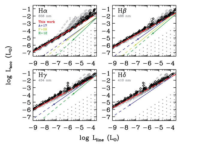
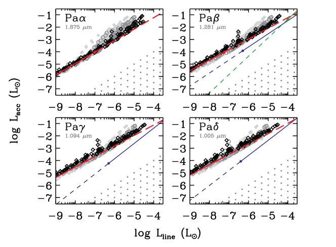
Figure 3: Correlation between line and accretion luminosities for hydrogen lines (see labels). Symbols show our model for the same $\dot{M}$ and $M_{\mathrm{p}}$ as in Figure 1 for $f_{\mathrm{fill}}=1$, 0.1, and 0.01 (black, dark gray, and pale gray symbols respectively) along with the fit (red line; Table 1) from the points with $L_{\mathrm{acc}}\leqslant 10^{-4}~{}L_{\odot}$ (solid). Where available, the fits of Alcalá et al. (2017, blue), Fang et al. (2009, lime), and Rigliaco et al. (2012, green) are shown (solid: where their data exists; dashed: extrapolation). A dot marks the transition between fits and extrapolations but in our case the latter hold everywhere as a lower limit. In the dotted region, $L_{\mathrm{line}}>L_{\mathrm{acc}}$, which is likely unphysical (see Section 2.1).

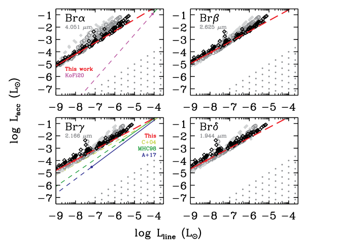
Figure 4: As in Figure 3 but for the first Brackett-series lines. The fit of Komarova & Fischer (2020, purple) is shown for Br $\alpha$ (observable with JWST), and those of Calvet et al. (2004, lime) and Muzerolle et al. (1998, green) for Br $\gamma$.

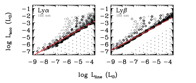
Figure 5: As in Figure 3 but for Ly $\alpha$ and Ly $\beta$. Lyman-series lines are less reliable than the others but are shown for completeness.

Figures 3–5 show our model results and the fits for several lines from the Balmer (H $\alpha$, H $\beta$, H $\gamma$, H $\delta$), Paschen (Pa $\alpha$, Pa $\beta$, Pa $\gamma$, Pa $\delta$), and Brackett (Br $\alpha$, Br $\beta$, Br $\gamma$, Br $\delta$) series, and also from the Lyman series (Ly $\alpha$, Ly $\beta$). In all cases, the fit to our results (red line) is roughly a lower limit. For the chosen range of input planet masses (2–20 $M_{\mathrm{J}}$) and excluding the Lyman-series lines, the half-spread in $L_{\mathrm{acc}}$ at a given $L_{\mathrm{line}}$ is often relatively small, with $\sigma\approx 0.3$ dex, but can reach $\sigma\approx 0.5$ dex. For the Lyman lines, the high optical depth of the upper layers of the postshock region lead to strong self-absorption. This is especially true for the points for lower planet masses, which have a higher density at a given $\dot{M}$ since $\rho\propto 1/v_{\mathrm{ff}}$.

For all transitions, our data is above the stellar relationship, for the $L_{\mathrm{line}}$ values covered both by their data and our model results, as well as where the stellar fit is extrapolated. The difference reaches up to 1–2 dex for the Balmer lines, especially compared to Rigliaco et al. (2012), and 2–3 dex for Paschen lines. For Br $\alpha$, the difference is extreme (2–4 dex) compared to the fit of Komarova & Fischer (2020). This is however not surprising because there is barely an overlap in $L_{\mathrm{acc}}$ between their data and our models, and their fit does not cover at all the $L_{\mathrm{line}}$ values relevant to planetary accretion ($L_{\mathrm{line}}\lesssim 10^{-5.5}~{}L_{\odot}$). In general, as discussed in Section 2.1, we do not expect the $L_{\mathrm{acc}}$–$L_{\mathrm{line}}$ relationships to match between the stellar and planetary regimes because the generating mechanisms probably differ significantly. Note that, except for the H $\alpha$ fit of Rigliaco et al. (2012), none of the extrapolations of the stellar fits reaches into the $L_{\mathrm{line}}>L_{\mathrm{acc}}$ region, which would be likely unphysical (Section 2.1).

References

- Alcalá et al. (2014) Alcalá, J. M., Natta, A., Manara, C. F., et al. 2014, A&A, 561, A2
- Alcalá et al. (2017) Alcalá, J. M., Manara, C. F., Natta, A., et al. 2017, A&A, 600, A20
- Aoyama & Ikoma (2019) Aoyama, Y., & Ikoma, M. 2019, ApJ, 885, L29
- Aoyama et al. (2018) Aoyama, Y., Ikoma, M., & Tanigawa, T. 2018, ApJ, 866, 84
- Aoyama et al. (2020) Aoyama, Y., Marleau, G.-D., Mordasini, C., & Ikoma, M. 2020, arXiv e-prints, arXiv:2011.06608
- Batygin (2018) Batygin, K. 2018, AJ, 155, 178
- Brittain et al. (2020) Brittain, S. D., Najita, J. R., Dong, R., & Zhu, Z. 2020, ApJ, 895, 48
- Calvet & Gullbring (1998) Calvet, N., & Gullbring, E. 1998, ApJ, 509, 802
- Calvet et al. (2004) Calvet, N., Muzerolle, J., Briceño, C., et al. 2004, AJ, 128, 1294
- Christensen et al. (2009) Christensen, U. R., Holzwarth, V., & Reiners, A. 2009, Nature, 457, 167
- Close (2020) Close, L. M. 2020, AJ, 160, 221
- Cugno et al. (2019) Cugno, G., Quanz, S. P., Hunziker, S., et al. 2019, A&A, 622, A156
- Dong et al. (2020) Dong, J., Jiang, Y.-F., & Armitage, P. 2020, arXiv e-prints, arXiv:2012.06641
- Drążkowska et al. (2019) Drążkowska, J., Li, S., Birnstiel, T., Stammler, S. M., & Li, H. 2019, ApJ, 885, 91
- Eriksson et al. (2020) Eriksson, S. C., Asensio Torres, R., Janson, M., et al. 2020, A&A, 638, L6
- Fang et al. (2009) Fang, M., van Boekel, R., Wang, W., et al. 2009, A&A, 504, 461
- Gravity Collaboration et al. (2020) Gravity Collaboration, Garcia Lopez, R., Natta, A., et al. 2020, Nature, 584, 547
- Gullbring et al. (1998) Gullbring, E., Hartmann, L., Briceño, C., & Calvet, N. 1998, ApJ, 492, 323
- Haffert et al. (2019) Haffert, S. Y., Bohn, A. J., de Boer, J., et al. 2019, Nature Astronomy, 329
- Hartmann et al. (2016) Hartmann, L., Herczeg, G., & Calvet, N. 2016, ARA&A, 54, 135
- Hartmann et al. (1994) Hartmann, L., Hewett, R., & Calvet, N. 1994, ApJ, 426, 669
- Hashimoto et al. (2020) Hashimoto, J., Aoyama, Y., Konishi, M., et al. 2020, AJ, 159, 222
- Herczeg et al. (2004) Herczeg, G. J., Wood, B. E., Linsky, J. L., Valenti, J. A., & Johns-Krull, C. M. 2004, ApJ, 607, 369
- Hummer & Storey (1987) Hummer, D. G., & Storey, P. J. 1987, MNRAS, 224, 801
- Ingleby et al. (2013) Ingleby, L., Calvet, N., Herczeg, G., et al. 2013, ApJ, 767, 112
- Komarova & Fischer (2020) Komarova, O., & Fischer, W. J. 2020, Research Notes of the American Astronomical Society, 4, 6
- Königl (1991) Königl, A. 1991, ApJ, 370, L39
- Landsman & Simon (1993) Landsman, W., & Simon, T. 1993, ApJ, 408, 305
- Lovelace et al. (2011) Lovelace, R. V. E., Covey, K. R., & Lloyd, J. P. 2011, AJ, 141, 51
- Lubow & Martin (2012) Lubow, S. H., & Martin, R. G. 2012, ApJ, 749, L37
- Marleau et al. (2017) Marleau, G.-D., Klahr, H., Kuiper, R., & Mordasini, C. 2017, ApJ, 836, 221
- Marleau et al. (2019) Marleau, G.-D., Mordasini, C., & Kuiper, R. 2019, ApJ, 881, 144
- Marleau et al. (subm.) Marleau, G.-D., Aoyama, Y., Kuiper, R., et al. subm., A&A
- Martin (1996) Martin, S. C. 1996, ApJ, 470, 537
- Mordasini et al. (2012) Mordasini, C., Alibert, Y., Georgy, C., et al. 2012, A&A, 547, A112
- Mordasini et al. (2017) Mordasini, C., Marleau, G.-D., & Mollière, P. 2017, A&A, 608, A72
- Muzerolle et al. (1998) Muzerolle, J., Calvet, N., & Hartmann, L. 1998, ApJ, 492, 743
- Muzerolle et al. (2001) Muzerolle, J., Calvet, N., & Hartmann, L. 2001, ApJ, 550, 944
- Owen & Menou (2016) Owen, J. E., & Menou, K. 2016, ApJ, 819, L14
- Rab et al. (2019) Rab, C., Kamp, I., Ginski, C., et al. 2019, A&A, 624, A16
- Rigliaco et al. (2012) Rigliaco, E., Natta, A., Testi, L., et al. 2012, A&A, 548, A56
- Sallum et al. (2015) Sallum, S., Follette, K. B., Eisner, J. A., et al. 2015, Nature, 527, 342
- Sanchis et al. (2020) Sanchis, E., Picogna, G., Ercolano, B., Testi, L., & Rosotti, G. 2020, MNRAS, 492, 3440
- Schulik et al. (2019) Schulik, M., Johansen, A., Bitsch, B., & Lega, E. 2019, A&A, 632, A118
- Schulik et al. (2020) Schulik, M., Johansen, A., Bitsch, B., Lega, E., & Lambrechts, M. 2020, A&A, 642, A187
- Storey & Hummer (1995) Storey, P. J., & Hummer, D. G. 1995, MNRAS, 272, 41
- Szulágyi et al. (2019) Szulágyi, J., Dullemond, C. P., Pohl, A., & Quanz, S. P. 2019, MNRAS, 487, 1248
- Szulágyi & Ercolano (2020) Szulágyi, J., & Ercolano, B. 2020, ApJ, 902, 126
- Szulágyi et al. (2014) Szulágyi, J., Morbidelli, A., Crida, A., & Masset, F. 2014, ApJ, 782, 65
- Szulágyi & Mordasini (2017) Szulágyi, J., & Mordasini, C. 2017, MNRAS, 465, L64
- Tanigawa & Ikoma (2007) Tanigawa, T., & Ikoma, M. 2007, ApJ, 667, 557
- Tanigawa et al. (2012) Tanigawa, T., Ohtsuki, K., & Machida, M. N. 2012, ApJ, 747, 47
- Teague et al. (2019) Teague, R., Bae, J., & Bergin, E. A. 2019, Nature, 574, 378
- Thanathibodee et al. (2019) Thanathibodee, T., Calvet, N., Bae, J., Muzerolle, J., & Hernández, R. F. 2019, ApJ, 885, 94
- Wagner et al. (2018) Wagner, K., Follete, K. B., Close, L. M., et al. 2018, ApJ, 863, L8
- Wang et al. (2021) Wang, J. J., Vigan, A., Lacour, S., et al. 2021, AJ, 161, 148
- Xie et al. (2020) Xie, C., Haffert, S. Y., de Boer, J., et al. 2020, A&A, 644, A149
- Zhou et al. (2014) Zhou, Y., Herczeg, G. J., Kraus, A. L., Metchev, S., & Cruz, K. L. 2014, ApJ, 783, L17
- Zhou et al. (2021) Zhou, Y., Bowler, B. P., Wagner, K. R., et al. 2021, AJ, 161, 244
- Zhu (2015) Zhu, Z. 2015, ApJ, 799, 16
- Zurlo et al. (2020) Zurlo, A., Cugno, G., Montesinos, M., et al. 2020, A&A, 633, A119