Probing Operator Spreading via Floquet Engineering in a Superconducting Circuit

Abstract

Operator spreading, often characterized by out-of-time-order correlators (OTOCs), is one of the central concepts in quantum many-body physics. However, measuring OTOCs is experimentally challenging due to the requirement of reversing the time evolution of systems. Here we apply Floquet engineering to investigate operator spreading in a superconducting 10-qubit chain. Floquet engineering provides an effective way to tune the coupling strength between nearby qubits, which is used to demonstrate quantum walks with tunable couplings, reversed time evolution, and the measurement of OTOCs. A clear light-cone-like operator propagation is observed in the system with multiple excitations, and has a nearly equal velocity as the single-particle quantum walk. For the butterfly operator that is nonlocal (local) under the Jordan-Wigner transformation, the OTOCs show distinct behaviors with (without) a signature of information scrambling in the near integrable system.

Introduction.—Spreading of quantum operators, probed by out-of-time-order correlators (OTOCs) [2, 3, 4, 5, 6, 7, 8, 9], is a new viewpoint to study the dynamics of quantum many-body systems. For instance, it is closely related to the Lieb-Robinson bound [10, 11] in local quantum systems and information scrambling in quantum chaotic systems  [2, 3, 4, 12, 13, 14, 15]. Given two local operators $\hat{W}$ and $\hat{V}$, the OTOC with a pure state $\ket{\psi_{0}}$ is defined as [6]

$$C(t)=\bra{\psi_{0}}\hat{W}(t)\hat{V}\hat{W}^{\dagger}(t)\hat{V}^{\dagger}\ket{\psi_{0}},$$ (1)

where $\hat{W}(t)=e^{i\hat{H}t}\hat{W}e^{-i\hat{H}t}$ is the butterfly operator, and $\hat{H}$ is the system Hamiltonian. The OTOC is related to the commutator between $\hat{W}(t)$ and $\hat{V}$. In a dynamical process, it usually starts from unity where two operators fully commute, and decays when they no longer commute and the system may become scrambled [7, 8]. To probe $C(t)$, one generally needs to reverse the time evolution of the system [5, 16, 17, 18, 19, 20, 12], which is experimentally very challenging [22]. In the digital quantum simulation paradigm [23, 24], the dynamics of quantum many-body systems can be digitalized via a series of quantum gates according to the Trotter-Suzuki decomposition, and the reversed time evolution can be easily implemented in a similar way. These have been investigated in various physical systems such as nuclear magnetic resonance  [16, 17], trapped ions [18, 19], and superconducting circuits [20]. On the other hand, it is efficient to encode the reversed dynamics of the target system with a fully-controllable quantum simulator, which is a task of analog quantum simulations [23, 24]. In the system with special symmetry, the reversal of time evolution is realized with a combined digital-analog scheme in superconducting circuits [12], which nevertheless cannot be simply generalized to other systems without the corresponding symmetry. Hence a method to encode the reversed time evolution of a quantum many-body system in a full analog quantum simulation paradigm is highly desirable.

Floquet engineering, using time-periodic driving, is a powerful tool for the coherent manipulation of quantum many-body states and the control of their dynamics. It has achieved a great success in cold atom systems [25] for a number of studies [26, 27, 28, 29, 30]. It has also been applied in superconducting circuits for realizing qubit switch [31], high-fidelity quantum gates [32], quantum state transfer [33], and the model of topological magnon insulators [34]. Floquet driving can be used to tune both the magnitude and phase of the coupling between nearby qubits, thus offering a possible way for reversing the dynamics of a quantum system [25], measuring OTOCs [5], and probing operator spreading.

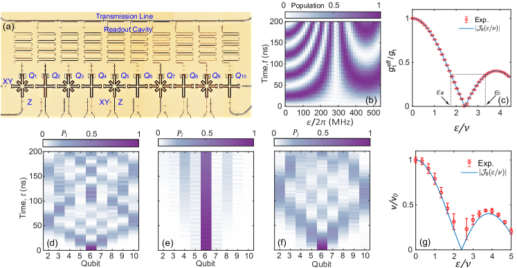
Figure 1: Device and quantum walk with tunable coupling. (a) Optical micrograph of the superconducting processor containing 10 transmon qubits arranged into a chain. Each qubit has a microwave line for the $XY$ control, a flux bias line for the $Z$ control, and a readout resonator for measurement. The NN qubits are coupled capacitively with almost the same strength [50]. The parameters of the device are presented in the Supplemental Material (SM) in detail [50]. (b) Experimental results of excitation oscillation between $Q_{1}$ and $Q_{2}$. The two qubits are prepared in the initial state of $\ket{01},$ and ac magnetic flux is applied on $Q_{1}$ with an amplitude $\varepsilon$. The color bar represents the expectation value of the photon number of $Q_{1}$. (c) Experimental coupling strength $g_{1}^{\text{eff}}$ versus ac magnetic flux amplitude $\varepsilon$, which satisfies $g_{j}^{\text{eff}}/g_{1}\approx\mathcal{J}_{0}(\varepsilon/\nu)$. Two arrows indicate the values, $\varepsilon_{a}$ and $\varepsilon_{b}$, used in the measurement of OTOCs for the forward and backward time evolution, respectively. Single-photon quantum walks for (d) $\varepsilon/2\pi=120$ MHz, (e) $\varepsilon/2\pi=288.6$ MHz, and (f) $\varepsilon/2\pi=400$ MHz, observed on $Q_{2}$-$Q_{10}$ with the initial state $\ket{000010000}$. (g) Normalized group velocity $v/v_{0}$ of photon propagation versus $\varepsilon/\nu$, where $v_{0}=117\pm 4$ sites/$\mu$s corresponds to the value with $\varepsilon=0$ [50]. The error bar is estimated by fitting errors. Each point is the average result of $8,000$ single-shot readouts.

In this Letter, we present a systematic study of operator spreading using Floquet engineering in a 1D array of 10 superconducting qubits. By precisely adjusting the ac magnetic flux at specific qubits, we are able to tune the coupling strength of nearby qubits and demonstrate the single-photon quantum walk with varying coupling, reversed time evolution, and the measurement of OTOCs. The Pauli operators $\hat{\sigma}^{z}$ and $\hat{\sigma}^{x}$ are taken as butterfly operators, which are local and nonlocal under the Jordan-Wigner transformation, respectively. We show that, with multiple excitations, a clear light-cone-like operator propagation can be observed with a velocity nearly equal to the group velocity of single-photon quantum walks. The OTOC with $\hat{W}$ = $\hat{\sigma}^{z}$ shows a revival to the initial value after a quick decay and finally approaches zero, which characterizes the nonthermalized process in the absence of scrambling. In contrast, no such revival is observed for the OTOC with $\hat{W}$ = $\hat{\sigma}^{x}$, showing a signature of scrambling. Our results demonstrate distinct behaviors of OTOCs in the nearly integrable system, some of which resemble those in nonintegrable chaotic systems [7, 8].

Experimental setup and protocol.—Superconducting qubits can be manipulated individually as well as simultaneously, which provide a convenient platform for simulating quantum many-body systems [40, 39, 35, 36, 37, 38, 41, 43, 6, 10, 45, 46, 47, 5, 49]. Our experiment is performed on a 1D array of 10 coupled transmon qubits, shown in Fig. 1(a). In the rotating frame with a common frequency, the system is described by the 1D Bose-Hubbard model [39, 6, 10]

$$\hat{H}(t)= \sum_{j=1}^{9}g_{j}(\hat{a}^{\dagger}_{j}\hat{a}_{j+1}+\text{h.c.})+\sum_{j=1}^{10}\omega_{j}(t)\hat{n}_{j}~{}~{}$$

$$+\sum_{j=1}^{10}\frac{U_{j}}{2}\hat{n}_{j}(\hat{n}_{j}-1),$$ (2)

where $\hat{a}^{\dagger}_{j}$ ($\hat{a}_{j}$) is the bosonic creation (annihilation) operator, $\hat{n}_{j}$ = $\hat{a}^{\dagger}_{j}\hat{a}_{j}$ is the number operator, $U_{j}$ is the on-site interaction, and $g_{j}$ is the nearest-neighbor (NN) coupling strength. In our experiment, we bias the qubit frequency with ac magnetic flux, i.e., we have $\omega_{j}(t)=\varepsilon_{j}\cos(\nu t)$, with $\nu$ and $\varepsilon_{j}$ being the ac frequency and amplitude, respectively. Thus $\hat{H}(t)$ describes a Floquet system satisfying $\hat{H}(t)=\hat{H}(t+T)$ with a period of $T=2\pi/\nu$  [50]. When $\nu\gg g_{j}$, under the hard-core boson approximation with $|U|\gg g_{j}$, we obtain an effective time-independent Hamiltonian [25]

$$\hat{H}_{\text{eff}}= \sum_{j=1}^{9}g_{j}^{\text{eff}}(\hat{\sigma}^{+}_{j}\hat{\sigma}^{-}_{j+1}+\hat{\sigma}^{+}_{j+1}\hat{\sigma}^{-}_{j})~{},$$ (3)

where $\hat{\sigma}^{\pm}=(\hat{\sigma}^{x}\pm i\hat{\sigma}^{y})/2$ with $\hat{\sigma}^{x,y,z}$ being Pauli matrices. The effective coupling strength has the form [25]

$$g_{j}^{\text{eff}}\approx g_{j}\mathcal{J}_{0}\big{(}\frac{\varepsilon_{j}-\varepsilon_{j+1}}{\nu}\big{)},$$ (4)

where $\mathcal{J}_{0}\big{(}x\big{)}$ is the Bessel function of order zero.

We tune the effective coupling strength between NN qubits by changing $\varepsilon_{j}$ with fixing $\nu/2\pi$ = 120 MHz. Figure 1(b) shows the experimental results of the excitation oscillation between $Q_{1}$ and $Q_{2}$, where the $\varepsilon$-dependent oscillation period can be seen. Using the Fourier transformation, we obtain the effective coupling strength as a function of $\varepsilon$, plotted in Fig. 1(c), which fits well with Eq. (4). In order to have a common coupling strength between each NN qubit pair, we only drive the odd qubits with the same amplitude $|\varepsilon_{j}|=\varepsilon$, so the coupling strength approximates $g_{j}\mathcal{J}_{0}(\varepsilon/\nu)$. In addition, we stagger the phase of the applied flux with $\varepsilon_{1},\varepsilon_{5},\varepsilon_{9}=\varepsilon$ and $\varepsilon_{3},\varepsilon_{7}=-\varepsilon$ to partly reduce the unwanted next-nearest-neighbor (NNN) coupling [50]. Hence we are able to set identical coupling strength for each NN qubit pair with adjustable values from positive to negative.

Quantum walks with tunable coupling.—The quantum walk is a fundamental process for quantum simulation and computation [6, 10, 51, 52, 53]. Figures 1(d)-(f) show the experimental observation in a 9-qubit system ($Q_{2}-Q_{10}$) with varying effective coupling strength. The experiment starts with all qubits biased at their idle points, and the central qubit $Q_{6}$ is excited from the ground state $\ket{0}$ to the first-excited state $\ket{1}$ by an $X_{\pi}$ gate to prepare an initial state $\ket{000010000}$ [50]. Afterwards, they are biased to the same frequency and the periodic driving is applied. The system then evolves with almost homogeneous coupling strength between NN qubits. The photon density distribution $P_{j}$ is measured after the system’s evolving for a time $t$, where $P_{j}(t):=\bra{\psi(t)}\hat{\sigma}^{+}_{j}\hat{\sigma}^{-}_{j}\ket{\psi(t)}$ with $\ket{\psi(t)}$ being the wave function at time $t$. Figure 1(d) shows the result for $\varepsilon/2\pi=120$ MHz, which displays a single-photon light-cone-like propagation [6, 10] in both the left and right directions.

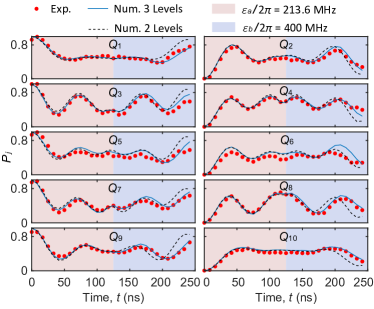
Figure 2: Reversed time evolution of the 10-qubit chain with the initial state $\ket{1010101010}$, realized by using $\varepsilon_{a}$ and $\varepsilon_{b}$ for the time before and after 125 ns, respectively. Symbols are the experimental results. Solid and dashed lines are the calculated results based on the Hamiltonian in Eq. (Probing Operator Spreading via Floquet Engineering in a Superconducting Circuit) by considering three and two energy levels for each qubit, respectively.

We find that the propagation velocity $v$ decreases with increasing $\varepsilon$ and vanishes at about $\varepsilon/2\pi\approx 288.6$ MHz ($\varepsilon/\nu\approx 2.4$), corresponding to the first zero of $\mathcal{J}_{0}$. At this point, the effective NN coupling reduces to zero, leading to dynamic localization [26, 27, 28] as illustrated in Fig. 1(e). Further increasing $\varepsilon$ results in reappearing of the linear propagation, see Fig. 1(f) for the case of $\varepsilon/2\pi=400$ MHz. In Fig. 1(g), we show the normalized group velocity $v/v_{0}$ versus $\varepsilon/\nu$, where $v_{0}$ = 117$\pm 4$ sites/$\mu$s is the value at $\varepsilon=0$. It can be seen that the data are also well described by the 0-th Bessel function, and the difference mainly originates from the unwanted NNN coupling [50]. Specifically, the group velocity for $\varepsilon/2\pi=400$ MHz is $v=46\pm 4$ sites/$\mu$s, which will be compared with the operator spreading velocity below. These results indicate a free single-photon propagation [6, 10] that is limited by the Lieb-Robinson bound [10, 11].

Reversed time evolution.—Reversing the dynamics of a quantum many-body system is of great interest and facilitates the OTOC measurement [6, 12]. Equation (4) indicates that the effective coupling $g_{j}^{\text{eff}}$ can be positive or negative. For single-photon quantum walks, the last term in Eq. (Probing Operator Spreading via Floquet Engineering in a Superconducting Circuit) vanishes, so the system is governed by the Hamiltonian (3). In this case, the time evolution can be precisely reversed by changing the sign of the Hamiltonian. However, OTOCs provide a technique for studying operator spreading and quantum information propagation in systems with multi-particle filling, which cannot be probed via single-particle propagation. Hence we will focus on the multi-photon system and discuss the effect of high-level occupations.

To observe the reversed time evolution, we choose the initial state as the Néel state $\ket{1010101010}$. The system evolves with a driving amplitude $\varepsilon=\varepsilon_{a}=213.6$ MHz for the first 125 ns and with $\varepsilon=\varepsilon_{b}=400$ MHz for the last 125 ns. Here we have $\mathcal{J}_{0}(\varepsilon_{a}/\nu)=-\mathcal{J}_{0}(\varepsilon_{b}/\nu)$, corresponding to $g_{j}^{\text{eff}}\approx\pm 4$ MHz for $\varepsilon_{a}$ and $\varepsilon_{b}$, respectively, as indicated by arrows in Fig. 1(c). The experimental results, plotted in Fig. 2 as symbols, are fairly reproduced by numerical simulations (lines). We can see that $P_{j}(t)$ is nearly symmetric about $t=125$ ns during the time evolution, demonstrating that two effective time-independent Hamiltonians are almost opposite in sign.

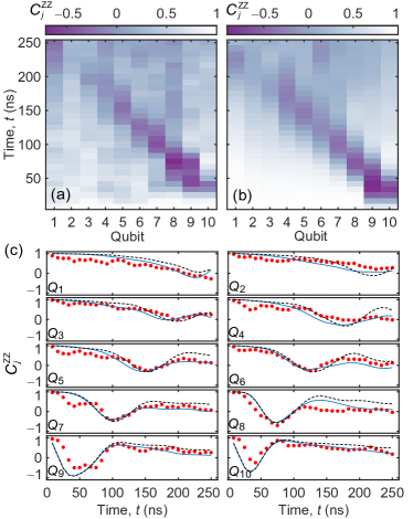
Figure 3: (a) Experimental results of $C_{j}^{\text{ZZ}}$, with the initial state $\ket{0101010101}$ and operators $\hat{W}=\hat{\sigma}^{z}_{10}$, $\hat{V}=\hat{\sigma}^{z}_{j}$ ($j$ = 1, …, 10). The post-selection is applied due to the $U(1)$ symmetry, i.e., only the single-shot results that have the same number of bosons as the initial state are considered. (b) Numerical results considering ZZ interaction between NN qubits. (c) Comparison between experimental $C_{j}^{\text{ZZ}}$ (symbols) and two calculated results using $\hat{H}_{\text{eff}}$ (dashed lines) and considering ZZ interaction (solid lines).

OTOCs and operator spreading.—To measure OTOCs and probe operator spreading, we consider two cases [7, 8]. First, we choose $\hat{W}=\hat{\sigma}^{z}_{10}$, $\hat{V}=\hat{\sigma}^{z}_{j}$ ($j$ = 1,…,10), and the initial state is $\ket{\psi_{1}}=\ket{0101010101}$. Since $\hat{V}\ket{\psi_{1}}=\hat{\sigma}^{z}_{j}\ket{\psi_{1}}=-(-1)^{j}\ket{\psi_{1}}$, from Eq. (1), the corresponding OTOC reads $C_{j}^{\text{ZZ}}(t)=-(-1)^{j}\bra{\phi_{z}(t)}\hat{\sigma}^{z}_{j}\ket{\phi_{z}(t)}$, where $\ket{\phi_{z}(t)}=\hat{\sigma}^{z}_{10}(t)\ket{\psi_{1}}$ [17]. Second, we let $\hat{W}=\hat{\sigma}^{x}_{10}$, $\hat{V}=\hat{\sigma}^{x}_{j}$ ($j$ = 1,…,10), and the initial state is $\ket{\psi_{2}}=\ket{++++++++++}$, where $\ket{+}$ is the eigenstate of $\hat{\sigma}^{x}$ with an eigenvalue $+1$. Similarly, the OTOC is measured as $C_{j}^{\text{XX}}(t)=\bra{\phi_{x}(t)}\hat{\sigma}^{x}_{j}\ket{\phi_{x}(t)}$, where $\ket{\phi_{x}(t)}=\hat{\sigma}^{x}_{10}(t)\ket{\psi_{2}}$ [17]. In the experiment, we first set $\varepsilon=\varepsilon_{a}$ and let the system evolve for a time $t$ from the initial state. Then we apply a $Z$ (or $X$) gate on $Q_{10}$ and let the system evolve reversely for time $t$ by setting $\varepsilon=\varepsilon_{b}$. Finally, we measure the observable $\hat{\sigma}^{z}_{j}$ (or $\hat{\sigma}^{x}_{j}$) to evaluate OTOC.

The experimental and numerical results of $C_{j}^{\text{ZZ}}$ are presented in Fig. 3. We can observe a clear light-cone-like operator propagation in Fig. 3(a). The velocity of operator spreading is calculated to be $40\pm 7$ sites$/\mu$s [50], which almost equals to the group velocity of single-photon quantum walks with the identical coupling strength. The small difference between these two velocities mainly comes from the NNN coupling, which enlarges the group velocity of single-photon quantum walks [50]. These results demonstrate that operator spreading with the local Hamiltonian is also limited by the Lieb-Robinson bound. The measured OTOCs are also plotted in Fig. 3(c) as symbols. They show a clear decay at the early stage and then revive almost back to the initial value of +1 for qubits near $Q_{10}$, which implies the absence of information scrambling. This can be explained considering that the effective Hamiltonian in Eq. (3) is integrable [4, 16]. It maps to free fermions under the Jordan-Wigner transformation and the $\hat{\sigma}^{z}$ operator does not change under the map. Finally, $C_{j}^{\text{ZZ}}$ gradually decays to zero at later time, indicating that $\ket{\phi_{z}(t)}$ tends to a steady state. Since the initial state is in the half-filling sector and $\ket{\phi_{z}(t)}$ is spin conserved, $C_{j}^{\text{ZZ}}$ represented by spin distribution will finally stabilize at zero.

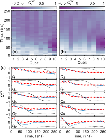
Figure 4: (a) Experimental results of $C_{j}^{\text{XX}}$ with the initial state $\ket{++++++++++}$ and operators $\hat{W}=\hat{\sigma}^{x}_{10}$, $\hat{V}=\hat{\sigma}^{x}_{j}$ ($j$ = 1, …, 10). (b) Numerical results considering the qubit third energy level. (c) Comparison between experimental $C_{j}^{\text{XX}}$ (symbols) and two numerical results using two (dashed lines) and three (solid lines) qubit levels.

These results show that OTOCs can well characterize the nonthermalized process and operator spreading in the multi-particle system. The effect of the last term in Eq. (Probing Operator Spreading via Floquet Engineering in a Superconducting Circuit) can also be seen, where it is not time reversible under the Floquet driving leading to a discrepancy from ideal time reversal [12]. For the results in Fig. 2, numerical simulations show that the population of the second-excited state varies with a maximum value up to 10$\%$, as compared to those of the first-excited state around 50$\%$. In Fig. 2, we present two results calculated by three- and two-level approximation of $\hat{H}(t)$, respectively. The result considering three levels is closer to experimental data. For the OTOC results in Fig. 3, where the post-selection is used, we take into account the influence of the third level through ZZ interaction [11, 12]. In Fig. 3(c), we can find that this numerical result is closer to experimental data than those calculated using $\hat{H}_{\text{eff}}$ in Eq. (3) [50].

The corresponding results of $C_{j}^{\text{XX}}$ are shown in Fig. 4. A significant difference from $C_{j}^{\text{ZZ}}$ is that no similar revival back to +1 is observed, which suggests the presence of scrambling with the $\hat{\sigma}^{x}$ butterfly operator [7, 8]. In the results, several features are blurred due to the high level participation [12]. The solid lines in Fig. 4(c) are the results calculated by considering the qubit third level [50], showing a satisfactory fit to experimental data. In addition, the results calculated by using two levels (dashed lines) demonstrate clear properties that $C_{j}^{\text{XX}}$ would have: First, the wavefront of OTOC can be better defined and propagates to the other edge of the qubit chain at a time nearly equal to that for $C_{j}^{\text{ZZ}}$. Second, $C_{j}^{\text{XX}}$ decreases at early times from +1 to -1 and almost retains in the rest of time range up to 250 ns. Here, the difference between butterfly operators $\hat{\sigma}^{z}$ and $\hat{\sigma}^{x}$ is that the former is local under the Jordan-Wigner transformation, whereas the latter maps to nonlocal Pauli-string operators giving rise to the behavior characteristic of scrambling [7, 8]. We emphasize that the scrambling here is fundamentally different from that in nonintegrable systems, in which it persists in a long timescale [4]. For both integrable and nonintegrable systems, the length of the string operators would increase linearly until approaching the system size. Afterwards, it will start to decrease and saturate for the two systems, respectively [3]. In SM [50], we show the periodic behavior of $C_{j}^{\text{XX}}$ by numerical simulation in a larger timescale, which demonstrates the existence of string operator shrinking in our near integrable system.

Summary and outlook.—We have used Floquet engineering, a full analog method, for probing operator spreading. Quantum walks with tunable coupling, reversed time evolution, and the measurement of OTOCs were demonstrated in a superconducting qubit chain. We observed a linear propagation of quantum operator with a velocity nearly equal to the group velocity of single-photon quantum walk, and also found that the OTOCs behave differently between $\hat{\sigma}^{z}$ and $\hat{\sigma}^{x}$ butterfly operators. The method may have further applications for the simulation of quantum many-body physics, e.g., quantum information scrambling and thermalization in nonintegrable systems  [2, 3, 4, 12, 13, 14, 15], dynamics of systems with weak integrability breaking  [55, 56], artificial gauge field  [29], topological band theory [57], and topological edge mode [50] in the Su-Schrieffer-Heeger model [13].

I Supplemental Material for
Probing Operator Spreading via Floquet Engineering in a Superconducting Circuit

This Supplemental Material contains four sections. In the first section, we present further experimental details of this work, including device information, measurement setup and method, readout calibration, single-qubit gate fidelity, and Z pulse and phase calibrations. Then we discuss some nonideal aspects and calculational details of our system, and their influence on the velocities of single-photon quantum walk and operator spreading. The experimental observation of the topologically protected edge mode in the Su-Schrieffer-Heeger model using Floquet engineering will be demonstrated in the last section.

II Experimental Details

II.1 Device information

Our superconducting 10-qubit sample is shown in Fig. S1 at the bottom (see also Fig. 1(a) in the main text), in which the qubits are transmons in the Xmon form [2, 3]. The device was fabricated on a $10\times 10$ mm² sapphire substrate with a 430 $\mu$m thickness. An Al base layer of 100 nm in thickness covering the whole substrate surface was first e-beam evaporated and photolithographically patterned. Using the wet etching method, the base-layer structures, including transmission lines, microwave coplanar waveguide resonators, XY and Z control lines, and qubit capacitors were defined. Josephson junctions in the dc-SQUID loops for tuning the critical current and qubit frequency were fabricated by e-beam lithography and double-angle evaporations. A 65 nm thick Al bottom electrode was evaporated at an angle of $60^{\circ}$, and after oxidation in pure oxygen, a 100 nm thick Al counter electrode was deposited at $0^{\circ}$. Finally, after lift-off, airbridges [4] were fabricated to suppress parasitic modes as well as the crosstalk among the control lines. Similar device fabrication processes have been described elsewhere [5].

In the 10-qubit chain, the nearby qubits are capacitively coupled with approximately the same capacitance. The odd-number qubits have larger capacitance due to an additional small cross-shaped area of the capacitor electrodes (see Fig. 1(a) in the main text), so the maximum frequencies of the odd- and even-number qubits stagger. The basic device parameters are listed in Tab. 1. The frequency of the readout resonator $f_{\text{r}}$ ranges from 6.545 to 6.729 GHz, well located within the bandwidth of our Josephson parametric amplifier (JPA). The maximum qubit frequency $f_{\text{m}}$ varies between 5.097 and 5.895 GHz, and $f_{\text{i}}$ is the qubit frequency at idle point. The energy relaxation time $T_{1}$ and the dephasing time $T_{2}^{*}$ are both measured at the idle point. The coupling strength between two nearby qubits is measured by vacuum Rabi oscillation at the working point. The nearest-neighbor (NN) coupling strength $g_{j,j+1}$ is almost equal while the next-nearest-neighbor (NNN) coupling strength $g_{j,j+2}$ of the odd- and even-number qubits are different as a result of the different qubit capacitance. The anharmonicity $U$ of odd- and even-number qubits are also different. In the table, $F_{\text{g}}$ and $F_{\text{e}}$ are the readout fidelities of the ground and first-excited states, respectively.

II.2 Measurement setup and method

Our experimental setup is shown in Fig. S1, in which from left to right are the Z control (fast and dc), XY control, qubit readout (input and output), and Josephson parametric amplifier (JPA) control lines, respectively. The circuits include a series of attenuators, filters, dc-blocks, bias-Tees, circulators, and amplifiers. The Z control lines provide dc and fast signals for tuning the qubit frequency. The XY control lines send microwave pulses for the manipulation of the qubit state. For the simultaneous state readout of all 10 qubits, ten-tone microwave pulse signals targeting the 10 readout resonators can be sent through the transmission line and amplified successively by the JPA, high electron mobility transistor (HEMT), and room-temperature microwave amplifier, which are finally demodulated by the analog digital converter.

The qubit readout resonator frequencies are displayed in Fig. S2, together with the qubit maximum frequencies and the frequencies at the idle and working points. In our experiment, the single-photon quantum walk, reversed time evolution, and OTOCs are measured. For each measurement, all qubits are first biased at their respective idle points for sufficiently long time during which single gate operations are performed on certain qubits to prepare an initial state of the system. Then all qubits are brought to their common working point and Floquet driving is applied. The Floquet driving amplitude can be the same (for single-photon quantum walk) or different (for reversed time evolution and OTOC measurements) in this time evolution period or a Z-gate (or X-gate) operation is performed in the middle of the period (for OTOC measurements). At the end of this period, all qubits are brought back to their idle points for the final-state readout. The pulse sequences used for different experiments are presented in Fig. S3, in which three main steps for the implementation of the experiments, namely the initial-state preparation, Floquet driving and free evolution, and state readout, can be seen.

II.3 Readout calibration

The readout of the qubit state is performed at the qubit’s idle point with the duration time of demodulation 1.2 $\mu$s. Fig. S4(a) shows the gain profile of the JPA used in the experiment to improve the signal-to-noise ratio for the state readout. In our experiment, the idle point of each qubit is chosen in the vicinity of the qubit sweet point in order to have a longer dephasing time, which is also well away from the frequencies of other unwanted two-level systems to avoid their couplings. Meanwhile, the frequency difference between the nearest-neighbor qubits is set as large as possible to reduce their XY crosstalk. For the present study, simultaneous readout of all 10 qubits in the chain is required. In Fig. S4(b), we show the IQ data of such joint readout of the qubit states with high fidelities (see Tab. 1). In order to correct the errors from initial state preparation and decoherence during measurement, we use the calibration matrix to reconstruct the readout results, defined as

$$T_{j}=\left(\begin{array}[]{cc}F_{g,j}&1-F_{e,j}\\ 1-F_{g,j}&F_{e,j}\\ \end{array}\right)~{},$$ (S1)

where $F_{g,j}$ and $F_{e,j}$ are the readout fidelities of the $j$-th qubit after being well initialized in the ground and first-excited states, respectively (see Tab. 1). With the calibration matrix, the correct probability of different qubit states can be found [6]. Finally, in the experiment of OTOCs, the post selection is applied for the readout results based on the conservation of photon number and the constraint of the qubit computational subspace.

II.4 Single-qubit gate fidelity

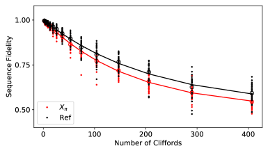
Figure S5: Randomized benchmarking result for $X_{\pi}$ gate measured on $Q_{2}$ with a gate fidelity of 99.93$\%$.

We use $X_{\pi}$ gate for the preparation of the excited state $\ket{1}$ for the selected qubits. Each $X_{\pi}$ gate contains two $X_{\pi/2}$ gates, which are accomplished by Gaussian-enveloped sinusoidal pulses with the length of 20 ns. The corresponding amplitude is optimized by repeating multiple sequences. The qubit frequencies are accurately determined by Ramsey interferometry measurement. In order to eliminate the phase error induced by the XY drive, we use AllXY sequence to optimize the DRAG factor [7]. Using the randomized benchmarking method (see Fig. S5 for the result of $Q_{2}$ as an example), we obtain the single-qubit gate fidelities, some of which are listed in Tab. 2.

II.5 Z pulse calibration and correction

In our experiment, various Z control line signals are required for different purposes for setting fixed qubit frequencies, performing gate operations, and producing a cosine-form oscillation for the qubit frequency with $\nu$=120 MHz. Below we describe the calibration of the Z pulse crosstalk, Z pulse shape correction, and optimized Z-gate operation, which are necessary for the precise qubit manipulations in the present experiment.

Due to the existing mutual inductance among the qubit control lines, the bias current applied on one qubit will also affect other qubits. In order to calibrate this Z pulse crosstalk, we first use dc bias to set a qubit $Q_{i}$ at a point in the energy spectrum that is sensitive to the flux, and excite it with a resonant microwave for 19 $\mu$s. At the same time, we scan the Z pulse amplitudes for $Q_{i}$ and another qubit $Q_{j}$ with the same pulse length of 20 $\mu$s. Since the qubit frequency changes linearly with respect to small offset, we expect that the position of the resonance peak also changes linearly with these two offsets. Hence the crosstalk matrix element for these two qubits can be found from the slope of the resonance peak plotted against the two offsets

$$c_{ij}=-\frac{\Delta f_{i}}{\Delta f_{j}},$$ (S2)

where $\Delta f_{i}$ is the frequency offset of $Q_{i}$. The measured crosstalk matrix is shown in Fig. S6(a).

As is shown in Fig. S1, starting from the DAC outputs, our Z control lines consist of differential amplifiers, bias-Tees, filters, and attenuators. Their limited bandwidth distorts the shape of Z pulse signals, which will in turn accumulate the unwanted phase error, as can be seen in the left panel of Fig. S6(b). We use the deconvolution method to correct the distortion. By scanning the shape of the Z pulse with $X_{\pi}$ gate, we can fit the peak to get the response function with respect to the control system. We predistort the shape of Z pulse on the basis of the response function for the correction [5]. In the right panel of Fig. S6(b), we show the shape of the Z pulse, which becomes flat, after the correction.

In the measurement of OTOCs, we need to perform a Z gate (phase-flip gate) or an X gate (bit-flip gate) operation on the tenth qubit $Q_{10}$, which is done at the idle point. At the same time, the phase accumulation for the other qubits during the operation should be avoided. This is realized by applying a Z gate to $Q_{10}$ and identity gates to the other qubits by Z pulses having the same duration as that of the Z gate pulse. To calibrate the different Z pulse amplitudes, we insert a Z pulse between two $X_{\frac{\pi}{2}}$ gates, change the amplitude (voltage) of the Z pulse, and readout the qubit population. The voltages of the Z pulse corresponding to the populations of 0 and 1 in the oscillating dependence reflect the Z pulse amplitudes required for the Z gate and identity, respectively. For more accurate determination, we insert an odd-number of identical Z pulses and readout the population again. The results for $Q_{1}$ are shown in Fig. S6(c) as an example. We choose the voltage indicated by the white (red) line as the parameter for the Z (identity) gate.

II.6 Calibration and correction of initial state phase and dynamical phase

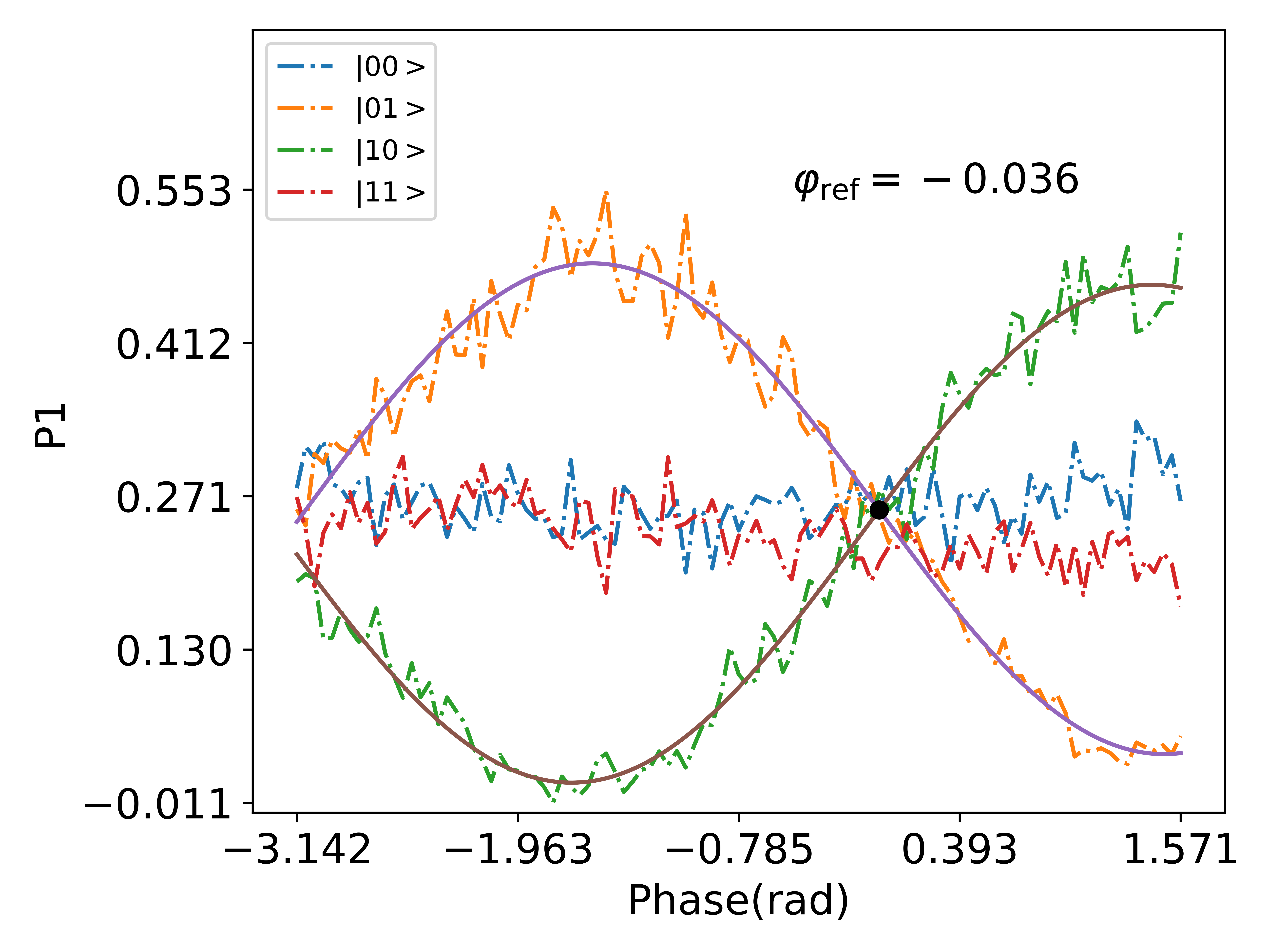
Figure S7: Calibration of the phase of the initial state. Curves with different colors label probabilities of four two-qubit computational basis. The solid lines are fits with cosine function. The black dot indicates the final reference phase $\varphi_{\rm ref}$ = -0.036.

In the preparation of the initial state $\ket{++++++++++}$ for the measurement of $C_{j}^{\text{XX}}$, we use a set of idle points ($f^{\prime}_{i}$) shown as dashed lines in Fig. S2, with larger separations between nearby qubits to reduce the effect of ZZ interaction, which is evaluated by Ramsey interference experiment [8]. The 10-qubit product state is prepared by $Y_{\frac{\pi}{2}}$ gates, see Fig. S3(d), where $\ket{+}=\frac{1}{\sqrt{2}}(\ket{0}+\ket{1})$. To make the $x$-axis of each Bloch sphere align, we calibrate and correct the phase of each XY driving with respect to the rotating frame of frequency $f^{\prime}_{i}$ [9]. For instance, we prepare the initial state of $Q_{1}$ and $Q_{2}$ as $\frac{1}{\sqrt{2}}(\ket{0}+e^{i\varphi_{\rm ref}}\ket{1})\otimes\frac{1}{\sqrt{2}}(\ket{0}+e^{i(\varphi+\varphi_{0})}\ket{1})$, where $\varphi_{0}$ originates from the phase difference between the two XY drivings. We choose $Q_{1}$ as the reference and fix $\varphi_{\rm ref}=0$. Then we set the two qubits at resonance at the working point $f_{w}$ for time $t=\frac{\pi}{4g_{j,j+1}}$. The two-qubit state will become $\frac{1}{2}\ket{00}+\frac{e^{i(\varphi+\varphi_{0})}+i}{2\sqrt{2}}\ket{01}+\frac{ie^{i(\varphi+\varphi_{0})}+1}{2\sqrt{2}}\ket{10}+\frac{e^{i(\varphi+\varphi_{0})}}{2}\ket{11}$. We adjust the phase $\varphi$ to have $\varphi+\varphi_{0}=0$, which gives equal probabilities of the four two-qubit computational basis. Finally, we choose $-\varphi_{0}$ as new $\varphi_{\rm ref}$ (black dot in Fig. S7) for correcting the phase between $Q_{2}$ and $Q_{3}$. The procedure is repeated pairwisely and successively to correct phases for all qubits in the initial state.

When the qubit frequency is biased away from the idle point by a Z pulse in the experiment, it deviates from the microwave frame and accumulates extra dynamical phase. We perform Ramsey-like measurement to determine the dynamical phase and make the compensation [5].

III Velocities of single-photon quantum walk and operator spreading

In the main text, we have mentioned that the group velocity of single-photon quantum walk is $\varepsilon$-dependent and equals the velocity of the operator spreading seen from $C_{j}^{\text{ZZ}}$ with the same coupling strength. Here we present the details for the evaluations of both velocities together with their error analysis.

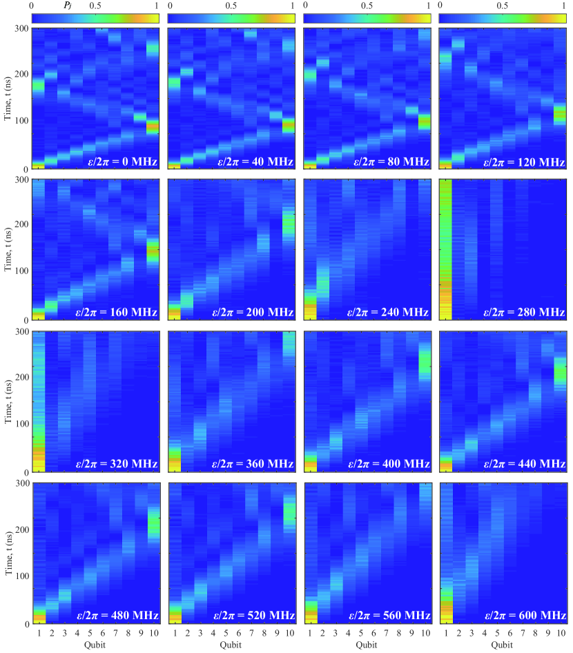
Figure S8: Experimental results of single-photon quantum walk of the 10-qubit chain under periodic driving with different $\varepsilon$. The initial state is $\ket{1000000000}$. Each point is the average result of $8,000$ single-shot readouts.

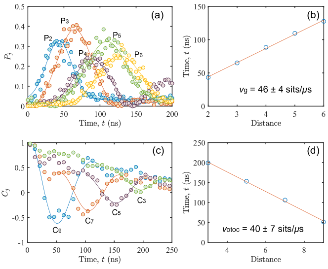
Figure S9: Fitting velocities of (a, b) single-photon quantum walk with $\varepsilon/2\pi=400$ MHz and corresponding coupling strength of 4 MHz, and (c,d) operator spreading with the same coupling strengths in absolute values.

In Fig. S8, we show the experimental results of single-photon quantum walks in the 10-qubit chain with varying $\varepsilon$ and an initial state of $\ket{1000000000}$. To obtain the group velocities [6, 10], we perform Gaussian fit to the data of $P_{2}(t)$–$P_{6}(t)$ and find the corresponding times of the first front of the fitting curves. Through a linear fit between the front time and qubit number, the group velocities can be obtained. In Fig. S9(a–b), we show an example for the result with $\varepsilon/2\pi=400$ MHz, for which the group velocity is calculated to be $v_{g}=46\pm 4$ sites/$\mu$s. For the experimental results of $C_{j}^{\text{ZZ}}$, the Gaussian fit is not applicable and the polynomial fit is used. Fig. S9(c) shows the experimental and fitting $C_{3}(t)$, $C_{5}(t)$, $C_{7}(t)$, $C_{9}(t)$. The front time of $C_{j}$ is plotted against qubit number in Fig. S9(d), from which the operator spreading velocity of $v_{\text{otoc}}=40\pm 7$ sites/$\mu$s is found.

For an isotropic $XY$ model in Eq. (3) with only NN coupling, one expects that the dynamics of the system can be perfectly reversed. Now we consider the influence of the existing nonideal NNN coupling and the high-level occupation that leads the system away from the ideal isotropic $XY$ model. We discuss how these two limitations affect the velocities of single-photon quantum walk and operator spreading seen from $C_{j}^{\text{ZZ}}$.

Tab. 1 shows that the NNN coupling strengths are about $1\times 2\pi$ MHz and $0.5\times 2\pi$ MHz for the odd- and even-site qubits, respectively. In order to partly suppress the NNN coupling, we apply ac magnetic flux on odd qubits with staggered phase, i.e., $\varepsilon_{1},\varepsilon_{5},\varepsilon_{9}=\varepsilon$ while $\varepsilon_{3},\varepsilon_{7}=-\varepsilon$. In this case, the effective coupling strength for the odd qubits becomes $\mathcal{J}_{0}(2\varepsilon/\nu)\times 2\pi$ MHz, while it does not change for the even qubits. This results in the reduced NNN coupling strength for the odd qubits. For instance, we have $\mathcal{J}_{0}(2\varepsilon/\nu)\approx-0.388$ for $\varepsilon/2\pi=213.6$ MHz and $\mathcal{J}_{0}(2\varepsilon/\nu)\approx 0.282$ for $\varepsilon/2\pi=400$ MHz, so the NNN coupling strength for the odd qubits becomes smaller compared to the original values.

For the discussion of $C_{j}^{\text{ZZ}}$ and operator spreading, we consider the qubit two-level subspace and take into account the influence of the second-excited state via the so-called ZZ interaction [11, 12]. Experimentally the post selection is applied for the measurement of OTOCs, where the high-level occupations of the final states are neglected. The Hamiltonian considering the ZZ interaction reads

$$\hat{H}^{\prime}=\hat{H}_{\text{eff}}+\epsilon\hat{H}_{\text{zz}}~{},$$

$$\hat{H}_{\text{zz}}=-\frac{1}{2}\sum_{j=1}^{9}(1+\hat{\sigma}^{z}_{j}\hat{\sigma}^{z}_{j+1})~{},$$ (S3)

where $\epsilon\sim g^{2}_{\text{eff}}/U\sim 0.065\times 2\pi$ MHz.

In Tab. 3, we compare the experimental velocities of single-photon quantum walk and operator spreading with the numerical ones with or without considering the NNN coupling and ZZ interaction. We can find that NNN coupling tends to enlarge the velocity of single-photon quantum walk, while the velocity of operator spreading is robust to the NNN coupling and ZZ interaction. In the last column of the table, a homogeneous XY chain with 25 spins and common NN coupling strength of $g$ MHz are considered. In this case, the two velocities are identical.

IV Numerical Calculation of $C_{j}^{\text{XX}}$

To explain experimental results of $C_{j}^{\text{XX}}$, we find that the qubit third level must be considered in numerical calculations during the entire dynamical process. Here, we replace the Pauli operator $\hat{\sigma}^{x}_{j}$ with

$$\hat{\Sigma}^{x}_{j}=\left(\begin{array}[]{ccc}0&1&0\\ 1&0&0\\ 0&0&\eta\\ \end{array}\right)~{}$$ (S4)

for the butterfly operator ($\eta$=1) and the measurement operator ($\eta$=0) in Eq. (6) in the main text. This implies that we neglect the third-level influence only in the readout. This treatment provides a reasonable description for the experimental $C_{j}^{\text{XX}}$.

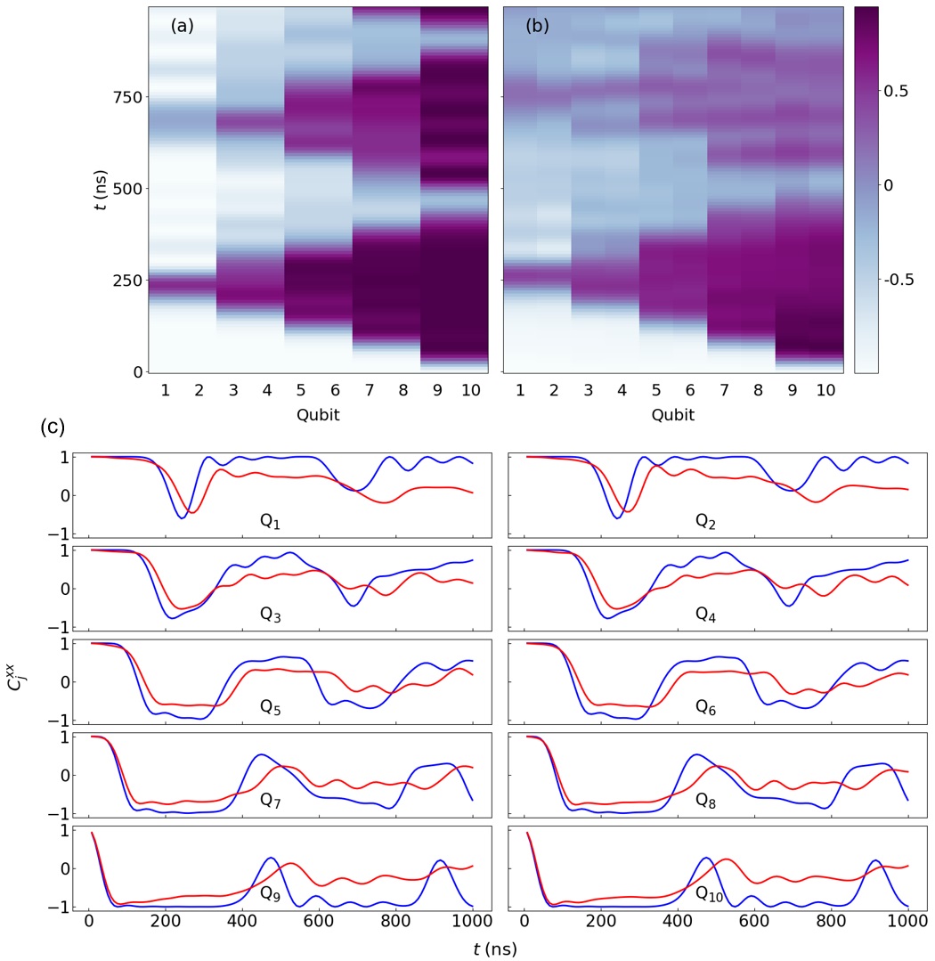
Figure S10: Numerical results of $C_{j}^{\text{XX}}$ by considering two levels. (a) Homogeneous NN coupling of 4 MHz without NNN coupling are considered, and time reversal is realized by directly changing the sign of NN coupling without Floquet driving. (b) With Floquet driving and using experimental parameters as described in the main text. The blue and red lines in (c) are the corresponding data in (a) and (b), in which the blurring of propagation features arising from NNN coupling and Floquet driving can be seen more clearly.

We also present the numerical result of $C_{j}^{\text{XX}}$ in a larger time scale without considering the qubit third level, see Fig. S10. The result without using Floquet driving or considering NNN coupling is also shown for comparison. These results demonstrate a nearly periodic behavior of $C_{j}^{\text{XX}}$ for the near integrable system and the blurring of propagation features arising from Floquet driving and NNN coupling.

V Su-Schrieffer-Heeger model and topologically protected edge mode

In the main text, we have used Floquet engineering to realize the homogeneous NN coupling for different studies. Here we demonstrate that the spatially periodic coupling strength in the qubit chain can be realized using the method for the study of the spin Su-Schrieffer-Heeger 1D compound lattice model [13] and its topological properties. To this end, we divide the 10-qubit chain into two sublattices labelled by $A$ and $B$, of which the Hamiltonian reads

$$\hat{H}_{\text{SSH}}=\sum_{j}(g_{o}^{\text{eff}}\hat{\sigma}^{+}_{A,j}\hat{\sigma}^{-}_{B,j}+g_{e}^{\text{eff}}\hat{\sigma}^{+}_{B,j}\hat{\sigma}^{-}_{A,j+1}+\text{H.c.}),$$ (S5)

where we label the odd-site qubit $Q_{2j-1}$ as site $(A,j)$ and even-site qubit $Q_{2j}$ as site $(B,j)$. We find that when the effective intracell coupling strength is larger than intercell coupling, i.e., $|g_{o}^{\text{eff}}|>|g_{e}^{\text{eff}}|$, the system is topologically trivial. On the other hand, when $|g_{o}^{\text{eff}}|<|g_{e}^{\text{eff}}|$, the system becomes topologically nontrivial with the emergence of topological edge modes.

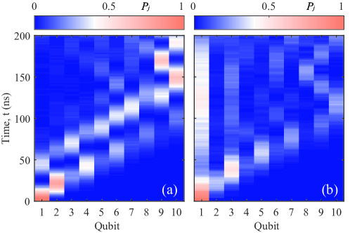
Figure S11: Quench dynamics of the SSH model. A driving amplitude $\varepsilon/2\pi=156$ MHz is used, and the photon is initially placed at the leftmost qubit $Q_{1}$. (a) The ac magnetic flux is applied on $Q_{3},\ Q_{4},\ Q_{7}$, and $Q_{8}$, where the effective time-independent Hamiltonian is topologically trivial. The photon can almost propagate freely. (b) The ac magnetic flux is applied on $Q_{2},\ Q_{3},\ Q_{6}$, $Q_{7}$, and $Q_{9}$, where the effective time-independent Hamiltonian is topologically nontrivial. The photon remains localized at the left edge. Each point is the average result of $8,000$ single-shot readouts.

Experimentally we Floquet drive $Q_{3},\ Q_{4},\ Q_{7}$, and $Q_{8}$ with the amplitude $\varepsilon/2\pi=156$ MHz, so the effective intracell coupling $g_{o}^{\text{eff}}=g_{2j-1,2j}$, and intercell coupling $g_{e}^{\text{eff}}\approx 0.5g_{2j,2j+1}<g_{o}^{\text{eff}}$. In Fig. S11(a), we present the measured quench dynamics of single excitation in this case. We can see that the single excitation is delocalized when initially placed at the left-most qubit $Q_{1}$, so the system is topologically trivial. Figure S11(b) shows the case when ac magnetic flux is applied on $Q_{2},\ Q_{3},\ Q_{6}$, $Q_{7}$, and $Q_{9}$ with the amplitude $\varepsilon/2\pi=156$ MHz. The system becomes topologically nontrivial in this case since the single excitation initially placed at the edge remains localized, which is a strong dynamical signature of the existence of topologically protected edge mode.

Supplemental Tables

	$Q_{1}$	$Q_{2}$	$Q_{3}$	$Q_{4}$	$Q_{5}$	$Q_{6}$	$Q_{7}$	$Q_{8}$	$Q_{9}$	$Q_{10}$
$f_{\text{r}}$ (GHz)	6.545	6.563	6.587	6.609	6.630	6.648	6.642	6.689	6.709	6.729
$f_{\text{m}}$ (GHz)	5.308	5.896	5.387	5.097	5.144	5.395	5.327	5.804	5.389	5.726
$f_{\text{i}}$ (GHz)	4.454	5.455	4.688	5.018	4.520	5.334	4.944	5.556	5.186	4.820
$f^{\prime}_{\text{i}}$ (GHz)	4.518	5.100	4.282	5.018	4.247	5.200	4.323	5.127	4.268	5.060
$U/2\pi$ (MHz)	-212	-264	-210	-268	-212	-268	-214	-264	-214	-264
$T_{1}$ ($\mu$s)	47.6	26.3	40.4	17.5	23	29.3	46	30.8	38.2	29.3
$T_{2}^{*}$ ($\mu$s)	1.97	2.34	1.74	6.36	2.12	36.7	2.63	3.79	3.51	1.54
$F_{\text{g}}$ (%)	97.2	99.2	99.2	99.7	98.1	99.4	99.3	99.4	99.3	99.3
$F_{\text{e}}$ (%)	90.4	92.6	92.4	90.7	90.3	91.7	89.9	91.7	92.5	85.6
$g_{j,j+1}/2\pi$ (MHz)	10.72     10.73     10.99     11.05     10.88     10.48     10.86     10.79     10.78
$g_{j,j+2}/2\pi$ (MHz)		0.98	0.49	0.96	0.49	0.96	0.49	0.97	0.48

Table 1: Basic device parameters. $f_{\text{r}}$ is the readout resonator frequency, $f_{\text{m}}$ is the qubit maximum frequency, and $f_{\text{i}}$ is the qubit idle frequency ($f^{\prime}_{\text{i}}$ is the idle frequency used only for the measurement of $C_{j}^{\text{XX}}$). $U$ is the qubit anharmonicity. $T_{1}$ and $T_{2}^{*}$ are the energy relaxation time and dephasing time of the qubit at idle point. $F_{\text{g}}$ and $F_{\text{e}}$ are the readout fidelities for the ground and first-excited states, respectively. $g_{j,j+1}$ and $g_{j,j+2}$ are the coupling strengths of nearest-neighbor (NN) and next-nearest-neighbor (NNN) qubits, respectively.

	$Q_{1}$	$Q_{2}$	$Q_{3}$	$Q_{4}$	$Q_{5}$	$Q_{6}$	$Q_{7}$	$Q_{8}$	$Q_{9}$	$Q_{10}$
$X_{\pi}(\%)$	99.81	99.93	99.91	99.89	99.84	99.92	99.76	99.96	99.88	99.59
$X_{\frac{\pi}{2}}(\%)$	99.91	99.95	99.89	99.97	99.87	99.98	99.40	99.87	99.71	99.81
$Y_{\frac{\pi}{2}}(\%)$	99.89	99.95	99.90	99.93	99.89	99.97	99.24	99.77	99.77	99.79

Table 2: Fidelities of single-qubit gates measured by the randomized benchmarking method. $X_{\theta}$ ($Y_{\theta}$) represents a rotation around the $x$- ($y$-) axis for an angle of $\theta$.

Velocity(sites/$\mu$s)	Exp.	NNN coupling	ZZ coupling	No NNN or ZZ coupling	Homogeneous
Quantum walk	$46\pm 4$	$50\pm 5$	$42\pm 2$	$42\pm 2$	$(1.85\pm 0.02)g$
Operator spreading	$40\pm 7$	$39\pm 9$	$39\pm 10$	$39\pm 10$	$(1.85\pm 0.02)g$

Table 3: Comparison of the velocities of single-photon quantum walk and operator spreading. In the last column, a homogeneous $XY$ chain with 25 spins and an NN coupling of $g_{j}=g$ MHz are considered.

Figure S1: Experimental setup. From left to right are the Z control (fast and dc), XY control, qubit readout (input and output), and JPA control lines, respectively. The XY and Z control lines are shown only for the third qubit $Q_{3}$ for simplicity.

Figure S2: Device frequency diagram. The green, blue, and red lines represent the readout resonator frequency $f_{r}$, qubit maximum frequency $f_{m}$, and qubit idle frequency $f_{i}$, respectively.The red dashed lines represent the idle frequency used only for the measurement of $C_{j}^{\text{XX}}$. The frequency of the qubit working point($f_{w}$) is shown with a long black dash-dotted line.

Figure S3: Pulse sequences for the experiments of (a) single-photon quantum walk, (b) reversed time evolution, (c) ZZ OTOC, and (d) XX OTOC. The orange, blue, and red pulses represent XY, Z, and readout drives, respectively.

Figure S4: Qubit-state readout. (a) The transmission spectra of the readout signals with JPA on (blue) and off (orange). (b) IQ data of the readout signals of the ground (blue) and first-excited (orange) states, where 10 qubits are measured simultaneously.

Figure S6: Z pulse calibration and correction. (a) Z pulse crosstalk matrix of the 10-qubit chain. (b) The original distorted Z pulse (left panel) and the one after correction (right panel). (c) Measured populations of $Q_{1}$ as functions of the amplitude and the number of Z pulses inserted between two $X_{\pi/2}$ gates. We choose the voltages indicated by the white (red) line as the pulse amplitude for the Z (identity) gate.

References

- [1]
- [2] J. Koch, T. M. Yu, J. Gambetta, A. A. Houck, D. I. Schuster, J. Majer, A. Blais, M. H. Devoret, S. M. Girvin, and R. J. Schoelkopf, “Charge-insensitive qubit design derived from the cooper pair box,” Phys. Rev. A 76, 042319 (2007).
- [3] R. Barends, J. Kelly, A. Megrant, D. Sank, E. Jeffrey, Y. Chen, Y. Yin, B. Chiaro, J. Mutus, C. Neill, P. O’Malley, P. Roushan, J. Wenner, T. C. White, A. N. Cleland, and J. M. Martinis, Coherent Josephson qubit suitable for scalable quantum integrated circuits, Phys. Rev. Lett. 111, 080502 (2013).
- [4] Z. Chen, A. Megrant, J. Kelly, R. Barends, J. Bochmann, Y. Chen, B. Chiaro, A. Dunsworth, E. Jeffrey, J. Y. Mutus, P. J. J. O‘Malley, C. Neill, P. Roushan, D. Sank, A. Vainsencher, J. Wenner, T. C. White, A. N. Cleland, and J. M. Martinis, Fabrication and characterization of aluminum airbridges for superconducting microwave circuits, Appl. Phys. Lett. 104, 052602 (2014).
- [5] X.-Y Guo, Z.-Y. Ge, H. Li, Z. Wang, Y.-R. Zhang, P. Song, Z. Xiang, X. Song, Y. Jin, L. Lu, K. Xu, D. Zheng, and H. Fan, Observation of Bloch oscillations and Wannier-Stark localization on a superconducting quantum processor, npj Quantum Inf. 7, 51 (2021).
- [6] Z. Yan, Y. R. Zhang, M. Gong, Y. Wu, Y. Zheng, S. Li, C. Wang, F. Liang, J. Lin, Y. Xu, C. Guo, L. Sun, C. Z. Peng, K. Xia, H. Deng, H. Rong, J. Q. You, F. Nori, H. Fan, X. Zhu, and J.-W. Pan, Strongly correlated quantum walks with a 12-qubit superconducting processor, Science 364, 753 (2019).
- [7] M. D. Reed, Entanglement and Quantum Error Correction with Superconducting Qubits, Ph.D. thesis (2013).
- [8] Jaseung Ku, Xuexin Xu, Markus Brink, David C. McKay, Jared B. Hertzberg, Mohammad H. Ansari, and B. L. T. Plourde. Suppression of Unwanted ZZ Interactions in a Hybrid Two-Qubit System, Phys. Rev. Lett. 125, 200504 (2020).
- [9] Chao Song, Kai Xu, Wuxin Liu, Chui-ping Yang, Shi-Biao Zheng,, Hui Deng, Qiwei Xie, Keqiang Huang, Qiujiang Guo, Libo Zhang, Pengfei Zhang, Da Xu, Dongning Zheng, Xiaobo Zhu, H. Wang, Y.-A. Chen, C.-Y. Lu, Siyuan Han, and Jian-Wei Pan, 10-Qubit Entanglement and Parallel Logic Operations with a Superconducting Circuit, Phys. Rev. Lett. 119, 180511 (2017).
- [10] Y. Ye, Z.-Y. Ge, Y. Wu, S. Wang, M. Gong, Y.-R. Zhang, Q. Zhu, R. Yang, S. Li, F. Liang, J. Lin, Y. Xu, C. Guo, L. Sun, C. Cheng, N. Ma, Z. Y. Meng, H. Deng, H. Rong, C.-Y. Lu, C.-Z. Peng, H. Fan, X. Zhu, and J.-W. Pan, Propagation and localization of collective excitations on a 24-qubit superconducting processor, Phys. Rev. Lett. 123, 050502 (2019).
- [11] D. C. McKay, C. J. Wood, S. Sheldon, J. M. Chow, and J. M. Gambetta, Efficient Z gates for quantum computing, Phys. Rev. A 96, 022330 (2017).
- [12] J. Braumüller, A.H. Karamlou, Y. Yanay, B. Kannan, D. Kim, M. Kjaergaard, A. Melville, B. M. Niedzielski, Y. Sung, A. Vepsäläinen, R. Winik, J. L. Yoder, T. P. Orlando, S. Gustavsson, C. Tahan, and W. D. Oliver, Probing quantum information propagation with out-of-time-ordered correlators, arXiv:2102.11751.
- [13] W. P. Su, J. R. Schrieffer, and A. J. Heeger, Solitons in Polyacetylene, Phys. Rev. Lett. 42, 1698 (1979).