Dissipationless Spin-Charge Conversion in Excitonic Pseudospin Superfluid

Abstract

Spin-charge conversion by inverse spin Hall effect or inverse Rashba-Edelstein effect is prevalent in spintronics but dissipative. We propose a dissipationless spin-charge conversion mechanism by an excitonic pseudospin superfluid in an electron-hole double layer system. Magnetic exchange fields lift singlet-triplet degeneracy of interlayer exciton levels in the double layer system. Condensation of the singlet-triplet hybridized excitons breaks both a U(1) gauge symmetry and a pseudospin rotational symmetry around the fields, leading to spin-charge coupled superflow in the system. We demonstrate the mechanism by deriving spin-charge coupled Josephson equations for the excitonic superflow from a coupled quantum-dot model.

Introduction.— Exploring novel approaches to information storage and transport is one of the major challenge in condensed matter physics and quantum information [1, 2, 3, 4]. Spintronics utilize spin degree of freedom of electrons [5, 6, 7, 8, 9, 10]. As spin voltage or spin current is hardly direct observable, efficient spin-charge conversion becomes a prerequisite for spintronics applications. Inverse spin Hall [11, 12, 13, 14, 15, 16] and Rashba-Edelstein [17, 18, 19, 20, 21, 22, 23] effects are widely used to convert spin current and spin voltage into charge current respectively. These effects are accompanied by diffusive quasiparticle transport so that the spin-charge conversions by them are generally lossy.

A dissipationless spin-charge conversion can be realized in superfluids that have both charge [24, 25] and spin [26, 27, 28, 29, 30, 31, 32, 33, 34, 35, 36, 37, 38, 39, 40, 41, 42, 43, 44, 45] superflow properties. Spin-triplet superconductors [46] and ferromagnetic Josephson junctions [47, 48, 49, 50, 51, 52] are among such systems, where spin-polarized Cooper pairs in superconductors are induced by spontaneous symmetry breakings or by magnetic proximity effects [53, 54, 55, 56, 57] from ferromagnetic interfaces. In ferromagnetic Josephson junctions, ferromagnetic moments in the interfaces control a relative superconducting phase between spin up and down Cooper pairs, leading to dissipationless Josephson charge and spin currents [48, 51]. Nonetheless, the relative phase is a massive mode. Thereby, the finite mass hinders the low-energy conversion from spin voltage to charge current.

Exciton condensates in two-dimensional (2D) electron-hole double-layer (EHDL) systems are ideal platforms for dissipationless conversion between spin voltage and charge current. In the 2D EHDL, electron and hole layers are separated from each other by an insulating layer [58, 59, 60, 61]. Electrons and holes interact only through Coulomb attraction, which binds them into bound states (excitons). In the presence of a spin-rotational symmetry in either one of the two layers, the bound states have an energy degeneracy between singlet and triplet excitonic pseudospin (electrons and holes with opposite spins) levels. Condensation of such excitons breaks not only a relative U(1) gauge symmetry between the two layers but also a pseudospin rotational symmetry, a combination of two spin rotational symmetries in the two layers. The broken gauge symmetry gives rise to electric supercurrents flowing in opposite directions in the two layers [62, 63, 58], while the broken pseudospin rotational symmetry leads to spin supercurrents. An experimental observation of the charge supercurrents without magnetic field remains illusive at this moment [60, 61, 64], while it has been observed in the quantum limit [65, 66, 67, 68, 69, 70, 71, 72].

In this paper, we propose a dissipationless spin-charge conversion in the 2D EHDL system under magnetic exchange fields. The exchange fields induce a polarization of an excitonic pseudospin. A condensate of such excitons break the pseudospin rotational symmetry around the exchange fields and the U(1) gauge symmetry, having two gapless Goldstone modes. We clarify relations among the pseudospin polarization, physical symmetries and the Goldstone modes in the condensate. We derive spin-charge coupled Josephson equations by a quantum-dot junction model [73, 74]. Based on the coupled Josephson equations, we show that a finite static spin voltage (a spatial gradient of the exchange field) leads to an unconventional time-dependent charge supercurrent, giving a microscopic mechanism of the dissipationless spin-charge conversion. We also clarify that SOC [75, 76] gives rise to spatial textures of the pseudospin polarization in the condensate [77], where the finite static spin voltage induces not only the charge supercurrent but also a dissipationless sliding of the textures.

Model.— The 2D EHDL system (in $xy$ plane) is described by a Hamiltonian ($\hat{H}$):

$$\hat{K} \equiv\hat{H}-\mu\hat{N}$$

$$=\int\mathrm{d}^{2}\vec{r}\bm{a}^{\dagger}(\vec{r})[(-\frac{\hbar^{2}\nabla^{2}}{2m_{a}}-E_{g})\bm{\sigma}_{0}+H_{a}\bm{\sigma}_{x}]\bm{a}(\vec{r})$$

$$+\int\mathrm{d}^{2}\vec{r}\bm{b}^{\dagger}(\vec{r})[(\frac{\hbar^{2}\nabla^{2}}{2m_{b}}+E_{g})\bm{\sigma}_{0}+H_{b}\bm{\sigma}_{x}]\bm{b}(\vec{r})$$

$$+g\sum_{\sigma,\sigma^{\prime}=\uparrow,\downarrow}\int\mathrm{d}^{2}\vec{r}\!\ a^{\dagger}_{\sigma}(\vec{r})b^{\dagger}_{\sigma^{\prime}}(\vec{r})b_{\sigma^{\prime}}(\vec{r})a_{\sigma}(\vec{r}).$$ (1)

Here $\bm{a}\equiv(a_{\uparrow},a_{\downarrow})$ and $\bm{b}\equiv(b_{\uparrow},b_{\downarrow})$ are annihilation operators of spin-1/2 electrons in the electron and hole layer with a positive effective mass $m_{a}$ and a negative effective mass $-m_{b}$ respectively. $2E_{g}$ is an energy difference between the bottom of the electron band and the top of the hole band. Electrons in both layers have chemical potential $\mu$, and $\hat{N}$ is a total number of electrons in the EHDL system. $H_{a}$ and $H_{b}$ are magnetic exchange fields in the two layers. The exchange fields can be experimentally induced by magnetic proximity effect from magnetic substrates. The interlayer interaction is modelled by a short-range interaction with a coupling constant $g$, while no tunneling between the two layers is allowed. The interaction leads to interlayer $s$-wave exciton pairing, that can be described by a four-component exciton pairing field $\phi_{\mu}\equiv\frac{g}{2}\expectationvalue{\bm{b}^{\dagger}\bm{\sigma}_{\mu}\bm{a}}$ with pseudospin singlet ($\mu=0$) and triplet ($\mu=x,y,z$) components. The exchange fields lift four-fold degeneracy of the exciton levels, which causes a singlet-triplet hybridization.

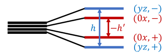
Figure 1: The four-fold spin degeneracy is lifted by the exchange fields. When $|h|>|h^{\prime}|$ ($|h|<|h^{\prime}|$), the lowest band is transverse (longitudinal) hybrid mode, where the pseudospin polarization is in the $yz$ ($0x$) plane. $(yz/0x,\pm)$ are exciton levels whose pseudospin polarization field $\vec{\phi}$ are in the $yz/0x$ plane and $\pm$ specifies a relative position between the real and imaginary part of the four-components exciton field $\vec{\phi}$ within the $yz/0x$ plane. The figure is for $h>-h^{\prime}>0$.

The hybdrization can be seen from a $\phi^{4}$-type effective Lagrangian for the four-component exciton pairing field $\vec{\Phi}\equiv(-\mathrm{i}\phi_{0},\phi_{x},\phi_{y},\phi_{z})$ [77, 78] derived from the Hamiltonian (Eq. (Dissipationless Spin-Charge Conversion in Excitonic Pseudospin Superfluid)):

$$\mathcal{L}= -\eta\vec{\Phi}^{\dagger}\cdot\partial_{\tau}\vec{\Phi}-\Big{(}\alpha-\frac{2}{g}\Big{)}|\vec{\Phi}|^{2}-\gamma\Big{[}\big{(}\vec{\Phi}^{\prime 2}\big{)}^{2}+\big{(}\vec{\Phi}^{\prime\prime 2}\big{)}^{2}$$

$$+6\vec{\Phi}^{\prime 2}\vec{\Phi}^{\prime\prime 2}-4\big{(}\vec{\Phi}^{\prime}\cdot\vec{\Phi}^{\prime\prime}\big{)}^{2}\Big{]}+\lambda|\nabla\vec{\Phi}|^{2}$$

$$-2h\big{(}\Phi^{\prime}_{y}\Phi^{\prime\prime}_{z}-\Phi^{\prime}_{z}\Phi^{\prime\prime}_{y}\big{)}+2h^{\prime}\big{(}\Phi^{\prime}_{0}\Phi^{\prime\prime}_{x}-\Phi^{\prime}_{x}\Phi^{\prime\prime}_{0}\big{)}+\mathcal{O}(H_{a/b}^{2}),$$ (2)

where $|\vec{\Phi}|^{2}\equiv\vec{\Phi}^{\dagger}\cdot\vec{\Phi}$ and $\tau$ is the imaginary time. Here $\vec{\Phi}^{\prime}$ and $\vec{\Phi}^{\prime\prime}$ are real and imaginary parts of the complex-valued four-component exciton field, i.e. $\vec{\Phi}\equiv\vec{\Phi}^{\prime}+{\rm i}\vec{\Phi}^{\prime\prime}$. $h$ and $h^{\prime}$ are weighted averages between the exchange fields in the electron and hole layers, while their coefficients as well as other parameters ($\eta,\alpha,\gamma,\lambda$) in the Lagrangian depend on detailed material properties. We assume that $\eta<0$, $\gamma<0$, and $\lambda>0$ [77].

The pseudospin degeneracy is lifted by the $h$ and $h^{\prime}$ terms (Fig. 1). Energy levels of the singlet-triplet hybridized modes depend on a competition between $h$ and $h^{\prime}$, which favor $\vec{\Phi}$ polarized within the $yz$ and $0x$ planes respectively. When a mass of the lowest hybridized mode becomes negative, the excitons undergo condensation. In the condensate phase with finite amplitude of $\vec{\Phi}$, the term $\gamma(\vec{\Phi}^{\prime}\cdot\vec{\Phi}^{\prime\prime})^{2}$ in the action competes with the exchange terms; the quartic term favors a parallel arrangement of $\vec{\Phi}^{\prime}$ and $\vec{\Phi}^{\prime\prime}$, while the two exchange terms favor a perpendicular arrangement. The competition results in a finite angle between $\vec{\Phi}^{\prime}$ and $\vec{\Phi}^{\prime\prime}$.

The nature of the excitonic condensate can be clarified by a minimization of an action $S=\int d\tau\mathrm{d}^{2}\vec{r}\mathcal{L}$ by a $\tau$-independent classical configuration [78]. For $|h|>|h^{\prime}|$, the action is minimized by a transverse configuration,

$$\vec{\phi}_{\perp}(\theta,\varphi,\varphi_{0}) =\rho\mathrm{cos}\theta(\mathrm{cos}\varphi_{0}\!\ {\vec{e}}_{y}+\mathrm{sin}\varphi_{0}\!\ {\vec{e}}_{z})$$

$$+\mathrm{i}\rho\mathrm{sin}\theta[\mathrm{cos}(\varphi+\varphi_{0})\!\ {\vec{e}}_{y}+\mathrm{sin}(\varphi+\varphi_{0})\!\ {\vec{e}}_{z}],$$ (3)

while for $|h|<|h^{\prime}|$, it is minimized by a longitudinal configuration,

$$\vec{\phi}_{\parallel}(\theta,\varphi,\varphi_{0}) =\rho[-\mathrm{sin}\theta\mathrm{cos}(\varphi+\varphi_{0})\!\ {\vec{e}}_{0}+\mathrm{cos}\theta\mathrm{sin}\varphi_{0}\!\ {\vec{e}}_{x}]$$

$$+\mathrm{i}\rho[\mathrm{cos}\theta\mathrm{cos}\varphi_{0}\!\ {\vec{e}}_{0}+\mathrm{sin}\theta\mathrm{sin}(\varphi+\varphi_{0})\!\ {\vec{e}}_{x}],$$ (4)

with $\rho\equiv\sqrt{h_{c}/(2|\gamma|)}$ and $h_{c}\equiv\alpha-2/g$. Here ${\vec{e}}_{\mu}$ $(\mu=0,x,y,z)$ are unit vectors in the four-component vector space. Note also the difference between two coordinate spaces, $\vec{\Phi}\equiv(-{\rm i}\phi_{0},\phi_{x},\phi_{y},\phi_{z})$ and $\vec{\phi}\equiv(\phi_{0},\phi_{x},\phi_{y},\phi_{z})$. Eqs. (Dissipationless Spin-Charge Conversion in Excitonic Pseudospin Superfluid, Dissipationless Spin-Charge Conversion in Excitonic Pseudospin Superfluid) are given in the latter coordinate space. $\varphi$ in the equations is the angle between $\vec{\Phi}^{\prime}$ and $\vec{\Phi}^{\prime\prime}$. $\theta$ defines a ratio between $|\vec{\Phi}^{\prime}|$ and $|\vec{\Phi}^{\prime\prime}|$ through $\tan\theta\equiv|\vec{\Phi}^{\prime\prime}|/|\vec{\Phi}^{\prime}|$. $\varphi$ and $\theta$ in Eqs. (Dissipationless Spin-Charge Conversion in Excitonic Pseudospin Superfluid, Dissipationless Spin-Charge Conversion in Excitonic Pseudospin Superfluid) form a loop of a minimum-energy degeneracy;

$$\tilde{h}\equiv\mathrm{sin}\varphi\mathrm{sin}2\theta={\sf{h}}\equiv\left\{\begin{array}[]{cc}h/h_{c}&{\rm for}\!\ \!\ \!\ \vec{\phi}_{\perp}\\ -h^{\prime}/h_{c}&{\rm for}\!\ \!\ \!\ \vec{\phi}_{\parallel}.\\ \end{array}\right.$$ (5)

We call the exciton condensate with one of these two configurations (“$\perp$” and “$\parallel$”) as transverse ($yz$) and longitudinal ($0x$) phases respectively. Both configurations have two arbitrary phase variables. One is $\varphi_{0}$, an overall rotational phase of the pseudospin vector within the $yz$ or $0x$ plane [78]. The other is a combination of $\theta$ and $\varphi$ that satisfies the constraint Eq. (5). These two are nothing but gapless Goldstone modes associated with broken continuous symmetries. A first-order transition happens at $|h|=|h^{\prime}|\neq 0$, where the general classical solution is given by a linear superposition of the two configurations [78].

Spontaneously Broken Symmetries.— Both $yz$ and $0x$ phases break the relative $U(1)$ gauge symmetry between the two layers. They also break the pseudospin rotational symmetry in which spins in the electron and hole layers are rotated around the field in the same and opposite direction(s) respectively. The two arbitrary phase variables in Eqs. (Dissipationless Spin-Charge Conversion in Excitonic Pseudospin Superfluid–5) correspond to the Goldstone modes associated with these symmetry breakings. In fact, they can be absorbed into the relative gauge transformation and the pseduospin rotation by way of a mean-field coupling, $\vec{\phi}_{\omega}(\theta,\varphi,\varphi_{0})\cdot\bm{a}^{\dagger}\vec{\bm{\sigma}}\bm{b}$ ($\omega=\perp,\parallel$). Namely, the coupling is invariant under spin rotations around the $x$ axis together with a change of $\varphi_{0}$ by $\delta\varphi_{0}$,

$$\vec{\phi}_{\omega}(\theta,\varphi,\varphi_{0})\rightarrow\vec{\phi}_{\omega}(\theta,\varphi,\varphi_{0}+\delta\varphi_{0}),\quad$$

$$\bm{a}\rightarrow\mathrm{e}^{\mathrm{i}\varphi_{a}\bm{\sigma}_{x}}\bm{a},\quad\bm{b}\rightarrow\mathrm{e}^{\mathrm{i}\varphi_{b}\bm{\sigma}_{x}}\bm{b}=\mathrm{e}^{\mp\mathrm{i}(\varphi_{a}+\delta\varphi_{0})\bm{\sigma}_{x}}\bm{b}.$$ (6)

Here the “$\mp$” signs in Eq. (Dissipationless Spin-Charge Conversion in Excitonic Pseudospin Superfluid) are for $\omega=\perp,\!\ \parallel$ respectively. The upper and lower signs in “$\pm$” and “$\mp$” in the remaining of this letter shall be for $\omega=\perp,\!\ \parallel$ respectively. The coupling is also invariant under the relative gauge transformation together with a combination of changes of $\theta$, $\varphi$ and $\varphi_{0}$ under the constraint Eq. (5),

$$\vec{\phi}_{\omega}(\theta,\varphi,\varphi_{0})\rightarrow\mathrm{e}^{\mathrm{i}\psi}\vec{\phi}_{\omega}(\theta,\varphi,\varphi_{0})\equiv\vec{\phi}_{\omega}(\theta(\psi),\varphi(\psi),\varphi_{0}(\psi)),$$

$$\bm{a}\rightarrow\mathrm{e}^{\mathrm{i}\psi_{a}}\bm{a},\quad\bm{b}\rightarrow\mathrm{e}^{\mathrm{i}\psi_{b}}\bm{b}=\mathrm{e}^{\mathrm{i}(\psi_{a}-\psi)}\bm{b}.$$ (7)

Here $(\theta(\psi),\varphi(\psi),\varphi_{0}(\psi))$ satisfies the constraint Eq. (5) for an arbitrary U(1) phase $\psi$. A continuous variation of $(\theta(\psi),\varphi(\psi),\varphi_{0}(\psi))$ as a function of $\psi$ is shown in Fig. 4 of the supplementary material [78]. To emphasize the dependence of $\vec{\phi}_{\omega}$ on the two variables of the Goldstone modes, we use $\vec{\phi}_{\omega}(\psi,\tilde{h},\varphi_{0})$ instead of $\vec{\phi}_{\omega}(\theta,\varphi,\varphi_{0})$ where $\tilde{h}$ is a massive mode defined in Eq. (5). We further omit $\tilde{h}$ from the arguments of $\vec{\phi}_{\omega}$ in the followings.

Coupled Josephson effects.— As an analogy to pure charge or spin superfluids [26, 33], the two Goldstone modes, $\varphi_{0}$ and $\psi$, are related to spin and charge supercurrents respectively. Without the exciton condensation, the electron and hole layers have a spin rotational symmetry:

$$\bm{d}\rightarrow\mathrm{e}^{\mathrm{i}\varphi_{d}\bm{\sigma}_{x}}\bm{d},\quad H_{d}\rightarrow H_{d}-\hbar\partial_{t}\varphi_{d},$$ (8)

and a U(1) gauge symmetry:

$$\bm{d}\rightarrow\mathrm{e}^{\mathrm{i}\psi_{d}}\bm{d},\quad V_{d}\rightarrow V_{d}-\hbar\partial_{t}\psi_{d},$$ (9)

where $\bm{d}=\bm{a}/\bm{b}$, $d=a/b$, $V_{a/b}$ and $H_{a/b}$ are electric potential and exchange field along $x$ in the electron/hole layer respectively. Spatial differences of $V_{a/b}/(-e)$ and $H_{a/b}/(-e)$ are defined to be charge voltage and spin voltage in the electron/hole layer, where $e$ is the unit charge. Eqs. (8, 9) in combination with Eqs. (Dissipationless Spin-Charge Conversion in Excitonic Pseudospin Superfluid, Dissipationless Spin-Charge Conversion in Excitonic Pseudospin Superfluid) suggest that in the excitonic condensate, the charge and spin voltage control time dependence of $\psi$ and $\varphi_{0}$ respectively. As shown below, the spatial differences of these two gapless phases lead to spin-charge coupled Josephson currents.

The spin-charge coupled Josephson effects can be derived by a quantum-dot junction model [73, 78]. The model comprises two domains and a junction between them. Each domain can be regarded as an EHDL quantum dot. The two domains ($j=1,2$) have exciton pairing $\vec{\phi}_{\omega}(\psi,\varphi_{0})$ $(\omega=\perp,\parallel)$ with different values of $\psi$ and $\varphi_{0}$, i.e. $\psi_{j}$ and $\varphi_{0j}$ ($j=1,2$). The charge and spin voltages change across the junction in the electron/hole layer by $V_{Ca/b}$ and $V_{Sa/b}$ respectively. $e|V_{Sa/b}|$ is assumed to be much smaller than the exchange fields $|H_{a/b}|$, so that variations of the gapped modes ($\rho$ and $\tilde{h}$) can be neglected. An action for the model is given by a functional of $V_{Cd}$, $V_{Sd}$, $\psi_{j}$ and $\varphi_{0j}$ ($d=a,b$, $j=1,2$), that takes a quadratic form of the annihilation operators in the electron and hole layers in the two domains, ${\bm{a}}_{j}({\vec{r}})$ ($j=1,2$) and ${\bm{b}}_{j}({\vec{r}})$ ($j=1,2$). The action comprises of two parts:

$$\mathcal{S}[\bm{a}_{j},\bm{a}^{\dagger}_{j},\bm{b}_{j},\bm{b}^{\dagger}_{j},\psi_{j},\varphi_{0j};V_{Cd},V_{Sd}]=\mathcal{S}_{T}[\bm{a}_{j},\bm{a}^{\dagger}_{j},\bm{b}_{j},\bm{b}^{\dagger}_{j}]$$

$$\hskip 28.45274pt+\mathcal{S}_{\mathrm{mf}}[\bm{a}_{j},\bm{a}^{\dagger}_{j},\bm{b}_{j},\bm{b}^{\dagger}_{j},\psi_{j},\varphi_{0j};V_{Cd},V_{Sd}],$$ (10)

where a mean-field part:

$$\mathcal{S}_{\mathrm{mf}}=\int\mathrm{d}\tau\sum_{j=1,2}\sum_{\alpha}$$

$$\big{\{} \bm{a}^{\dagger}_{j\alpha}[\hbar\partial_{\tau}+\bm{H}_{a\alpha}-\mu-\frac{\eta_{j}}{2}e(V_{Ca}+V_{Sa}\bm{\sigma}_{x})]\bm{a}_{j\alpha}$$

$$+ \bm{b}^{\dagger}_{j\alpha}[\hbar\partial_{\tau}+\bm{H}_{b\alpha}-\mu-\frac{\eta_{j}}{2}e(V_{Cb}+V_{Sb}\bm{\sigma}_{x})]\bm{b}_{j\alpha}$$

$$- [\vec{\phi}_{\omega}(\psi_{j},\varphi_{0j})\cdot{\bm{a}}^{\dagger}_{j\alpha}{\vec{\bm{\sigma}}}{\bm{b}}_{j\alpha}+{\rm h.c.}]\big{\}},$$ (11)

and a tunneling part:

$$\mathcal{S}_{T}=\int\mathrm{d}\tau\sum_{\alpha\beta}[\bm{a}^{\dagger}_{1\alpha}T^{(a)}_{\alpha\beta}\bm{a}_{2\beta}+\bm{b}^{\dagger}_{1\alpha}T^{(b)}_{\alpha\beta}\bm{b}_{2\beta}+\mathrm{h.c.}],$$ (12)

with $\eta_{1}=-\eta_{2}=1$, ${\bm{a}}_{j}({\vec{r}})\equiv\sum_{\alpha}u_{aj\alpha}({\vec{r}})\!\ {\bm{a}}_{j\alpha}$ and ${\bm{b}}_{j}({\vec{r}})\equiv\sum_{\alpha}u_{bj\alpha}({\vec{r}})\!\ {\bm{b}}_{j\alpha}$. Here $u_{dj\alpha}({\vec{r}})$ is the $\alpha$-th single-particle eigenstate of the kinetic energy part of Eq. (Dissipationless Spin-Charge Conversion in Excitonic Pseudospin Superfluid) for the electron/hole layer in the $j$-th domain region ($d=a/b$, $j=1,2$) with a proper boundary condition, together with its eigenenergy ${\bm{H}}_{d\alpha}\equiv E_{d\alpha}\bm{\sigma}_{0}+H_{d}\bm{\sigma}_{x}$. Tunneling matrices between the two domains are given by the single-particle eigenstates, $T^{(d)}_{\alpha\beta}\equiv\langle u_{d1\alpha}|{\cal T}^{(d)}|u_{d2\beta}\rangle$, where ${\cal T}^{(d)}$ is the kinetic energy part for the electron/hole layer in the junction region ($d=a/b$). We assume that ${\cal T}^{(d)}$ is free from spin or electron-hole mixing.

A perturbative treatment of the tunneling term in the junction model leads to an effective action of the Josephson junction [78]:

$$\mathcal{S}_{\mathrm{eff}}[\tilde{\psi},\tilde{\varphi}_{0},N_{C},N_{S};V_{C},V_{S}]$$

$$=\int\mathrm{d}\tau\bigg{[}N_{C}(-\mathrm{i}\hbar\dot{\tilde{\psi}}(\tau)-eV_{C})+N_{S}(\mp\mathrm{i}\hbar\dot{\tilde{\varphi}}_{0}(\tau)-eV_{S})$$

$$-\hbar I_{0}\bigg{(}\mathrm{cos}\big{(}\tilde{\psi}-\frac{e}{\hbar c}\Psi\big{)}\mathrm{cos}\tilde{\varphi}_{0}+\bar{h}_{\pm}\mathrm{sin}\big{(}\tilde{\psi}-\frac{e}{\hbar c}\Psi\big{)}\mathrm{sin}\tilde{\varphi}_{0}\bigg{)}\bigg{]},$$ (13)

with $V_{C}\equiv V_{Cb}-V_{Ca}$, $V_{S}\equiv V_{Sb}\pm V_{Sa}$, $\tilde{\varphi}_{0}\equiv\varphi_{01}-\varphi_{02}$, $\tilde{\psi}\equiv\psi_{1}-\psi_{2}$, $\dot{\tilde{\varphi}}_{0}\equiv\partial_{\tau}\tilde{\varphi_{0}}$ and $\dot{\tilde{\psi}}\equiv\partial_{\tau}\tilde{\psi}$. $c$ is the speed of light. $N_{C}$ and $N_{S}$ are differences of total charge and spin between the two domains in the hole layer respectively [78]. $\Psi$ is an external magnetic flux trapped in the junction region. $I_{0}$ and $\bar{h}_{\pm}$ are constants and $\bar{h}_{\pm}$ is proportional to a weighted average of $H_{a}$ and $H_{b}$, while $\bar{h}_{+}\neq\bar{h}_{-}$. Spin currents are defined as differences of charge currents contributed by spin-up and spin-down electrons. By analyses of current directions in the two layers, the currents have relations:

$$I_{C}\equiv I_{Cb}= -I_{Ca}=e\partial_{t}N_{C},$$

$$I_{S}\equiv I_{Sb}= \pm I_{Sa}=e\partial_{t}N_{S},$$ (14)

where $I_{Ca/b}$ and $I_{Sa/b}$ are charge currents and spin currents in the electron/hole layer respectively. Josephson equations can be derived by minimization of Eq. (Dissipationless Spin-Charge Conversion in Excitonic Pseudospin Superfluid) with Eq. (Dissipationless Spin-Charge Conversion in Excitonic Pseudospin Superfluid) and Wick rotation ($\tau=\mathrm{i}t$) [78]. The first Josephson equations are:

$$I_{C}= -eI_{0}[\mathrm{sin}(\tilde{\psi}-\frac{e}{\hbar c}\Psi)\mathrm{cos}\tilde{\varphi}_{0}-\bar{h}_{\pm}\mathrm{cos}(\tilde{\psi}-\frac{e}{\hbar c}\Psi)\mathrm{sin}\tilde{\varphi}_{0}],$$ (15)

$$\pm I_{S}= -eI_{0}[\mathrm{sin}\tilde{\varphi}_{0}\mathrm{cos}(\tilde{\psi}-\frac{e}{\hbar c}\Psi)-\bar{h}_{\pm}\mathrm{cos}\tilde{\varphi}_{0}\mathrm{sin}(\tilde{\psi}-\frac{e}{\hbar c}\Psi)].$$ (16)

The second Josephson equations are:

$$\frac{\mathrm{d}\tilde{\psi}}{\mathrm{d}t}=-\frac{e}{\hbar}V_{C},\quad\frac{\mathrm{d}\tilde{\varphi}_{0}}{\mathrm{d}t}=\mp\frac{e}{\hbar}V_{S}.$$ (17)

The Josephson equations reveal spin-charge coupled Josephson effects. The term proportional to ${\rm sin}(\tilde{\psi}-\frac{e}{\hbar c}\Psi)$ in Eq. (15) and the term proportional to ${\rm sin}(\tilde{\varphi}_{0})$ in Eq. (16) represent the well-known pure charge and pure spin Josephson effects [79, 33, 80], while they are modulated by the spin phase ($\tilde{\varphi}_{0}$) and the charge phase ($\tilde{\psi}$) respectively. Moreover, the terms proportional to $\bar{h}_{\pm}$ in Eqs. (15, 16) indicates that a pure spin (charge) phase difference can still lead to a charge (spin) supercurrent, as the excitons are polarized by the exchange fields. In a trilayer ferromagnetic Josephson junction of superconductors, a relative angle between two ferromagnetic polarizations in two sides of a ferromagnetic junction plays a similar role to the spin phase [48, 51]. Differently, Eq. (17) further shows control of the spin phase by the spin voltage.

Device setup.— To propose the spin-charge conversion in a feasible experimental setup, we consider to put two magnetic substrates with different magnetizations along the same ($x$) direction under the hole layer (Fig. 2(a)). The two substrates introduce the two domains in the EHDL system, whose hole layers experience the magnetic exchange fields through the proximity effect. The difference of the exchange fields results in a finite d.c. spin voltage $V_{S}$ across the junction in the hole layer. The d.c. spin voltage results in a linear increase of $\tilde{\varphi}_{0}$, $\tilde{\varphi}_{0}=\mp\frac{e}{\hbar}V_{S}t$ ($\tilde{\varphi}_{0}=0$ at $t=0$ is taken without loss of generality). The time dependence of $\tilde{\varphi}_{0}$ gives rise to a.c. electric currents in counter-propagating directions in the electron and hole layers respectively. The electric currents induce the a.c. charge voltages across the junction in the electron and hole layers as $I_{Ca}R_{a}$ and $I_{Cb}R_{b}$, where $R_{a}$ and $R_{b}$ are external resistances (Fig. 2(a)). The exciton U(1) phase $\tilde{\psi}$ couples only with the difference between the charge voltages in the two layer, $V_{C}=I_{Ca}R_{a}-I_{Cb}R_{b}$. Thus, Eqs. (15, 17) give an equation of motion (EOM) for $\tilde{\psi}$:

$$I_{C}(s)\frac{R}{V_{S}}=\frac{\mathrm{d}\tilde{\psi}}{\mathrm{d}s}=-k[\mathrm{sin}(\tilde{\psi})\mathrm{cos}(s)\pm\bar{h}_{\pm}\mathrm{cos}(\tilde{\psi})\mathrm{sin}(s)],$$ (18)

with $R\equiv R_{a}+R_{b}$, a normalized time $s\equiv eV_{S}t/\hbar$, two dimensionless parameters, $k\equiv eI_{0}R/V_{S}$ and $\overline{h}_{\pm}$.

Solutions of the EOM are obtained numerically in the supplementary material [78]. $\tilde{\psi}(s)$ shows an oscillating behavior with a double-sine form for $|\bar{h}_{\pm}|<1/|k|$, and a stepping behaviour for $|\bar{h}_{\pm}|>1/|k|$ (Fig. 2(b)). $\tilde{\psi}(s)$ has an oscillatory component with $2\pi$ periodicity in $s$. The $\bar{h}_{\pm}$ term with $\mp k\bar{h}_{\pm}>0\!\ (<0)$ gives rise to a component of $\tilde{\psi}(s)$ that increases (decreases) linearly in the time $s$ and an additional longer oscillatory periodicity over which $\tilde{\psi}(s)$ increases (decreases) by $\pi$. When the longer periodicity approaches the shorter periodicity, the oscillating behavior shows a crossover to the stepping behavior. The double-sine form appears because the electric charge current is induced not only by a sine of the charge phase $\tilde{\psi}$ but also by another sine of the spin phase $\tilde{\varphi}_{0}$. The spin voltage $V_{S}$ can be measured from the (short) period of the a.c. electric current (Fig. 2(b)).

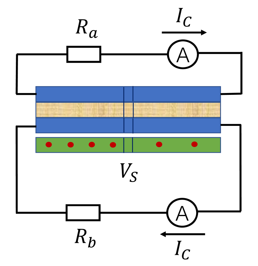
(a)

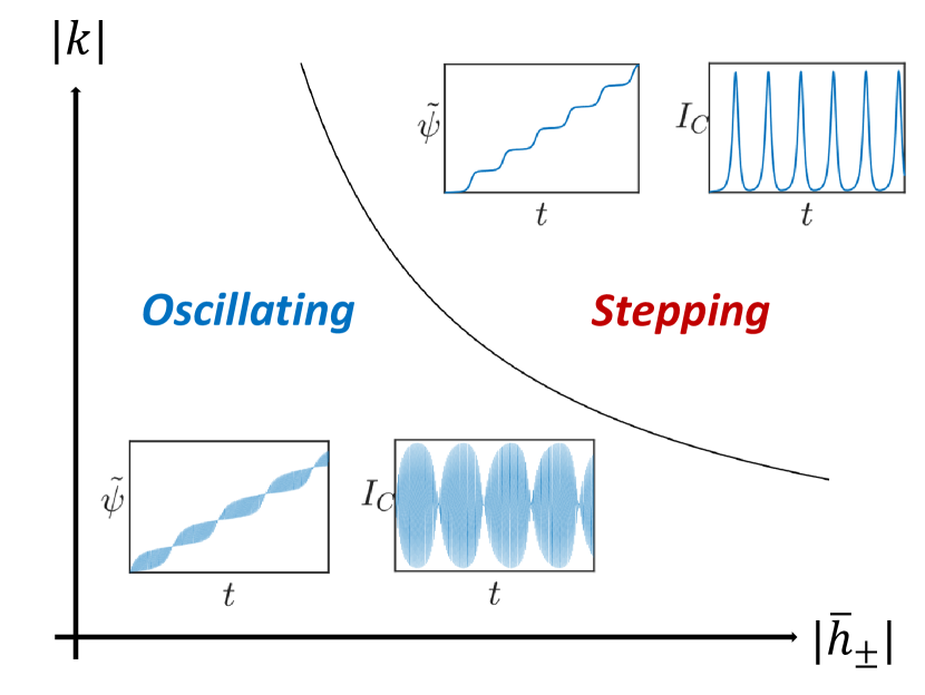
(b)

Figure 2: The charge current ($I_{C}$) induced by the spin voltage ($V_{S}$). (a) The spin voltage is added at the Josephson junction in the hole layer. The charge currents can be measured by the two external circuits attached to the electron and hole layers respectively. (b) The a.c. behavior of $\tilde{\psi}(t)$ and $I_{C}(t)$ according to Eq. (18) for small $|\bar{h}_{\pm}|$. $\tilde{\psi}(t)$ shows an oscillating behavior for $|\bar{h}_{\pm}k|<1$ and a stepping behavior for $|\bar{h}_{\pm}k|>1$.

Spin-orbit coupling.— A semiconductor hetetrostructure of the 2D EHDL systems breaks a spatial inversion symmetry, causing an effective Rashba SOC in the electron layer [75, 76, 81, 82]. The Rashba SOC endows the excitonic pseudospin polarizations with a nonzero momentum $K$ in a direction perpendicular to the exchange fields; $\varphi_{0}$ in Eqs. (Dissipationless Spin-Charge Conversion in Excitonic Pseudospin Superfluid, Dissipationless Spin-Charge Conversion in Excitonic Pseudospin Superfluid) is replaced by $\varphi_{0}-Ky$ [77, 78]. The condensate with the broken traslational symmetry also have the relative U(1) phase ($\psi$) and the spin rotational phase ($\varphi_{0}$) as low-energy Goldstone modes. The spin rotational phase $\varphi_{0}$ appears together with the spatial coordinate ($y$), so that it is also a translational phase (phason). The gapless $\varphi_{0}$ phase originates purely from the spin-rotational symmetry in the hole layer. Charge and (hole-layer) spin voltages control these two gapless modes respectively (Eq. (17)), while spatial gradients of these two modes generate charge and spin currents as well [78]. Accordingly, the dissipationless spin-charge conversion property is robust against the presence of the Rashba SOC.

Summary.— In this letter, we clarify the spin-charge coupled Josephson effects in the EHDL exciton system under magnetic exchange fields, where the charge Josephson current can be a response to the spin voltage. The spin-charge coupling effects provide a dissipationless way of the spin-charge conversion in a feasible device setup.

Supplementary Material for “Dissipationless Spin-Charge Conversion in Excitonic Pseudospin Superfluid”

In the main text, the $\phi^{4}$-type effective Lagrangian is introduced for the four-component excitonic fields. The $\phi^{4}$-type Lagrangian is derived from Eq. (1) perturbatively in the exchange fields. The Lagrangian is minimized in terms of a classical solution of the excitonic fields, leading to the prediction of transverse and longitudinal phases. Both of them are excitonic pseudospin superfluid phases. Using a coupled quantum dots model or the effective Lagrangian, we derive spin-charge coupled Josephson equations in these excitonic pseudospin superfluid phases. We also discuss the robustness of the spin-charge conversion against the Rashba spin-orbit coupling (SOC) in an electron layer. In this supplementary material, we explain these derivations and minimizations as well as related details.

The structure of this supplementary material is as follows. In the next section, we review possible forms of relativistic SOCs in 2D semiconductor heterostructures for the EHDL systems. In Sec. .2, we give the perturbative derivation of the $\phi^{4}$-type effective Lagrangian with the Rashba SOC. In Sec. .3, we describe the minimization of the Lagrangian without the SOC, where the classical ground-state phase diagram of transverse and longitudinal phases are presented. In Sec. .4 and .5, we clarify what global continuous symmetries are broken in the transverse and longitudinal phases, and we associate the broken symmetries with the gapless Goldstone modes in these phases. In Sec. .6, we derive the spin-charge coupled Josephson equations based on the coupled quantum dots model. In Sec. .7, we describe solutions of the Josephson equation under a physical experimental setup. In Sec. .8, we describe the minimization of the Lagrangian with the Rashba SOC in the electron layer, where a classical ground-state phase diagram of helicoidal and helical phases are presented. In Sec. .9, we derive the spin-charge coupled Josephson equation with the Rashba SOC, using Noether’s theorem for the $\phi^{4}$-type effective Lagrangian. In Sec. .10 and Sec. .11, we give supplementary details of Sec. .6 and Sec. .8 respectively.

There are some notation simplifications in this supplementary material. We take $\hbar=c=e=1$ unless dictated otherwise (we recover these fundamental physical constants in the very last expressions of important physical equations).

.1 Spin-orbit couplings (SOCs) in 2D semiconductor heterostructure systems

For a 2D semiconductor heterostructure of the EHDL systems, an effective confinement potential along $z$ direction may break spatial inversion symmetry. This kind of the broken spatial inversion symmetry is called structural inversion asymmetry (SIA). The SIA results in an effective electric field along $z$ direction, which leads to Rashba SOC in the electron layer;

$$\hat{H}_{R}=\xi_{e}\int\mathrm{d}^{2}\vec{r}\bm{a}^{\dagger}(\vec{r})(-\mathrm{i}\partial_{y}\bm{\sigma}_{x}+\mathrm{i}\partial_{x}\bm{\sigma}_{y})\bm{a}(\vec{r}),$$ (.1.1)

where $\xi_{e}$ is a strength of the Rashba coupling. The SIA in the electron-hole double-layer semiconductor systems results not only in the Rashba coupling in the electron layer with $S_{z}=\pm 1/2$, but also Rashba coupling in the hole layer with $J_{z}=\pm 3/2$. As the Pauli matrices ${\bm{\sigma}}_{x}$ and ${\bm{\sigma}}_{y}$ connect between the $J_{z}=\pm 3/2$ Kramers doublet in the hole layer, the SOC for the hole layer is proportional to a cubic in the momentum $k$ and atomic spin-orbit interaction strength and it is therefore negligibly small especially around the $\Gamma$ point. In addition to the SIA, the bulk crystal structure itself may break spatial inversion symmetry. The bulk inversion asymmetry (BIA) leads to Dirac-type SOC term in the hole layer of the EHDL systems [77, 76, 81]:

$$\hat{H}_{D}=\Delta_{h}\int d^{2}\vec{r}{\bm{b}}^{\dagger}(\vec{r})\big{(}-\mathrm{i}\partial_{x}{\bm{\sigma}}_{x}-\mathrm{i}\partial_{y}{\bm{\sigma}}_{y}\big{)}{\bm{b}}(\vec{r}).$$ (.1.2)

For a typical semiconductor heterostructure system, however, the Dirac-type SOC is still quantitatively negligible, $\Delta_{h}\sim 0.01\xi_{e}$[84, 82]. In this paper, we thus consider only the Rashba SOC in the electron layer and study how it changes the nature of the excitonic condensate (Sec. .8) and whether it influences the dissipationless spin-charge conversion property or not (Sec. .9).

.2 Derivation of $\phi^{4}$ type effective Lagrangian

In this section, we describe a derivation of the effective Lagrangian from the Hamiltonian Eq. (1) in the main text with the Rashba SOC, Eq. (.1.1). The derivation is perturbative in the exchange fields in Eq. (1) and in the Rashba coupling in Eq. (.1.1). Since both the exchange fields and the Rashba coupling are often much smaller than the typical energy scale of the electron and hole bands, we include only their first-order perturbation effect.

The partition function of the four-components exciton pairing fields $\vec{\phi}_{\mu}=\frac{g}{2}\langle{\bm{b}}^{\dagger}{\bm{\sigma}}_{\mu}{\bm{a}}\rangle$ ($\mu=0,x,y,z$) can be derived from Eq. (1) together with the Rashba coupling in the electron band (Eq. (.1.1));

$$Z=\int\mathcal{D}\phi^{\dagger}\mathcal{D}\phi\mathrm{exp}\{-\frac{2}{g}|\vec{\phi}|^{2}+\mathrm{Tr}[G_{0}G^{-1}_{R}G_{0}\Psi G_{0}\Psi+G_{0}G^{-1}_{H}G_{0}\Psi G_{0}\Psi-\frac{1}{2}G_{0}\Psi G_{0}\Psi-\frac{1}{4}G_{0}\Psi G_{0}\Psi G_{0}\Psi G_{0}\Psi]\},$$ (.2.1)

where

$$G^{-1}_{0}(q)\equiv\left(\begin{array}[]{cc}(-\mathrm{i}\omega_{n}+\mathcal{E}_{a}(\vec{k})-\mu)\bm{\sigma}_{0}&0\\ 0&(-\mathrm{i}\omega_{n}+\mathcal{E}_{b}(\vec{k})-\mu)\bm{\sigma}_{0}\end{array}\right)\equiv\left(\begin{array}[]{cc}{g^{0}_{a}}^{-1}(k)&0\\ 0&{g^{0}_{b}}^{-1}(k)\\ \end{array}\right),$$ (.2.2)

$$G^{-1}_{R}(q)\equiv\left(\begin{array}[]{cc}\xi_{e}(k_{y}\bm{\sigma}_{x}-k_{x}\bm{\sigma}_{y})&0\\ 0&0\end{array}\right),\qquad G^{-1}_{H}(q)\equiv\left(\begin{array}[]{cc}H\bm{\sigma}_{x}&0\\ 0&H\bm{\sigma}_{x}\end{array}\right),$$ (.2.3)

$$\Psi(q)=\frac{1}{\sqrt{\beta V}}\left(\begin{array}[]{cc}0&-\vec{\phi}(-k)\cdot\vec{\sigma}\\ -\vec{\phi}^{*}(k)\cdot\vec{\sigma}&0\end{array}\right),$$ (.2.4)

with $\mathcal{E}_{a}(\vec{k})\equiv\frac{\hbar^{2}\vec{k}^{2}}{2m_{e}}-E_{g}$, $\mathcal{E}_{b}(\vec{k})\equiv-\frac{\hbar^{2}\vec{k}^{2}}{2m_{h}}+E_{g}$, $q\equiv(\mathrm{i}\omega_{n},\vec{k})$ and $\vec{k}=(k_{x},k_{y})$. The expansion is perturbative in the excitonic field $\Psi(q)$, the Rashba coupling $G^{-1}_{R}(q)$ and the exchange fields $G^{-1}_{H}(q)$. From the gauge symmetry, the expansion contains only the even order in $\Psi(q)$. For the 2nd order in $\Psi(q)$, we expand the exchange fields and the Rashba coupling up to the first order. We ignore their effect in the quartic order in $\Psi(q)$.

The expansion has been previously carried out only for triplet-components excitonic field in Ref. [77]. In the following, we describe the expansion for singlet-component as well. $\mathrm{Tr}^{\prime}[...]$ denotes an additional contribution from the singlet-component $\phi_{0}\bm{\sigma}_{0}$,

$${\rm Tr}^{\prime}\big{[}\cdots\big{]}\equiv{\rm Tr}\big{[}\cdots\big{]}-{\rm Tr}\big{[}\cdots\big{]}_{\phi_{0}=0},$$ (.2.5)

and $\hat{\phi}$ and $\hat{\bm{\sigma}}$ denote the three-component (spin-triplet) vectors. The leading-order terms in the expansion are as follows:

$$\mathrm{Tr}^{\prime}[G_{0}G_{R}^{-1}G_{0}\Psi G_{0}\Psi]=-\mathrm{i}D\int\mathrm{d}\tau\mathrm{d}^{2}\vec{r}\!\ \vec{e}_{z}\cdot[(\hat{\phi}^{*}\times\nabla)\phi_{0}-\phi_{0}^{*}(\nabla\times\hat{\phi})],$$ (.2.6)

$$\mathrm{Tr}^{\prime}[G_{0}G_{H}^{-1}G_{0}\Psi G_{0}\Psi]=-h^{\prime}\int\mathrm{d}\tau\mathrm{d}^{2}\vec{r}\!\ \vec{e}_{x}\cdot(\phi_{0}^{*}\hat{\phi}+\phi_{0}\hat{\phi}^{*}),$$ (.2.7)

$$\mathrm{Tr}^{\prime}[-\frac{1}{4}(G_{0}\Psi)^{4}]=\gamma\int\mathrm{d}\tau\mathrm{d}^{2}\vec{r}\!\ [|\phi_{0}|^{4}+4|\phi_{0}|^{2}|\hat{\phi}|^{2}+(\phi_{0}^{*})^{2}(\hat{\phi})^{2}+(\phi_{0})^{2}(\hat{\phi}^{*})^{2}],$$ (.2.8)

$$\mathrm{Tr}^{\prime}[-\frac{1}{2}G_{0}\Psi G_{0}\Psi]=\alpha\int\mathrm{d}\tau\mathrm{d}^{2}\vec{r}\!\ |\phi_{0}|^{2}+\eta\int\mathrm{d}\tau\mathrm{d}^{2}\vec{r}\!\ \phi_{0}^{*}\partial_{\tau}\phi_{0}+\lambda\int\mathrm{d}\tau\mathrm{d}^{2}\vec{r}\!\ \phi_{0}^{*}\nabla^{2}\phi_{0}.$$ (.2.9)

These terms share the same coefficients as those in the leading-order terms in Ref. [77], except for $h^{\prime}$. For the later convenience, we give the expressions of $D$, $h$ and $h^{\prime}$ as follows:

$$D=-\frac{2\xi_{e}}{\beta V}\frac{\hbar^{2}}{m_{b}}\sum_{k}k^{2}_{x}g^{0}_{a}(k)^{2}g^{0}_{b}(k)^{2},$$ (.2.10)

$$h=\frac{2}{\beta V}\sum_{k}g^{0}_{a}(k)g^{0}_{b}(k)(H_{b}g^{0}_{b}(k)-H_{a}g^{0}_{a}(k)),$$ (.2.11)

$$h^{\prime}=\frac{2}{\beta V}\sum_{k}g^{0}_{a}(k)g^{0}_{b}(k)\big{[}H_{a}g^{0}_{a}(k)+H_{b}g^{0}_{b}(k)\big{]}=-\frac{2}{V}\sum_{\vec{k}}\frac{\beta}{\mathcal{E}_{a}-\mathcal{E}_{b}}[\frac{H_{a}}{2+2\mathrm{cosh}\beta(\mathcal{E}_{a}-\mu)}-\frac{H_{b}}{2+2\mathrm{cosh}\beta(\mathcal{E}_{b}-\mu)}].$$ (.2.12)

Putting Eqs. (.2.6–.2.9) into Eq. (.2.1) and add them into the triplet component (Eq. (5) of Ref. [77]), we obtain the $\phi^{4}$-type effective Lagrangian for the four-components excitonic field:

$$S =\int\mathrm{d}\tau\mathrm{d}^{2}\vec{r}\!\ \{-\eta\vec{\phi}^{\dagger}\partial_{\tau}\vec{\phi}+\lambda|\nabla\vec{\phi}|^{2}-(\alpha-\frac{2}{g})|\vec{\phi}|^{2}-\gamma[2|\hat{\phi}|^{4}-(\hat{\phi}^{*})^{2}(\hat{\phi})^{2}+|\hat{\phi}_{0}|^{4}+4|\phi_{0}|^{2}|\hat{\phi}|^{2}+(\phi_{0}^{*})^{2}(\hat{\phi})^{2}+(\phi_{0})^{2}(\hat{\phi}^{*})^{2}]$$

$$-D[\vec{e}_{y}\cdot(\hat{\phi}^{*}\times\partial_{x}\hat{\phi})-\vec{e}_{x}\cdot(\hat{\phi}^{*}\times\partial_{y}\hat{\phi})-\mathrm{i}\vec{e}_{z}\cdot((\hat{\phi}^{*}\times\nabla)\phi_{0}-\phi_{0}^{*}(\nabla\times\hat{\phi}))]+\mathrm{i}h\vec{e}_{x}\cdot(\hat{\phi}^{*}\times\hat{\phi})+h^{\prime}\vec{e}_{x}\cdot(\phi_{0}^{*}\hat{\phi}+\phi_{0}\hat{\phi}^{*})\},$$ (.2.13)

where $\vec{\phi}\equiv(\phi_{0},\hat{\phi})=(\phi_{0},\phi_{x},\phi_{y},\phi_{z})$, and $\nabla=(\partial_{x},\partial_{y},0)$. In terms of $\vec{\Phi}\equiv(-\mathrm{i}\phi_{0},\hat{\phi})\equiv\vec{\Phi}^{\prime}+\mathrm{i}\vec{\Phi}^{\prime\prime}$, the Lagrangian takes a more symmetric form:

$$S =\int_{0}^{\beta}\mathrm{d}\tau\int\mathrm{d}^{2}\vec{r}\{-\eta\vec{\Phi}^{\dagger}\partial_{\tau}\vec{\Phi}-(\alpha-\frac{2}{g})|\vec{\Phi}|^{2}-\gamma[(\vec{\Phi}^{\prime 2})^{2}+(\vec{\Phi}^{\prime\prime 2})^{2}+6\vec{\Phi}^{\prime 2}\vec{\Phi}^{\prime\prime 2}-4(\vec{\Phi}^{\prime}\cdot\vec{\Phi}^{\prime\prime})^{2}]+\lambda[(\nabla\vec{\Phi}^{\prime})^{2}+(\nabla\vec{\Phi}^{\prime\prime})^{2}]$$

$$-D(\Phi^{\prime}_{z}\partial_{x}\Phi^{\prime}_{x}-\Phi^{\prime}_{x}\partial_{x}\Phi^{\prime}_{z}+\Phi^{\prime}_{z}\partial_{y}\Phi^{\prime}_{y}-\Phi^{\prime}_{y}\partial_{y}\Phi^{\prime}_{z})-D(\Phi^{\prime}_{0}\partial_{x}\Phi^{\prime}_{y}-\Phi^{\prime}_{y}\partial_{x}\Phi^{\prime}_{0}+\Phi^{\prime}_{x}\partial_{y}\Phi^{\prime}_{0}-\Phi^{\prime}_{0}\partial_{y}\Phi^{\prime}_{x})$$

$$-D(\Phi^{\prime\prime}_{z}\partial_{x}\Phi^{\prime\prime}_{x}-\Phi^{\prime\prime}_{x}\partial_{x}\Phi^{\prime\prime}_{z}+\Phi^{\prime\prime}_{z}\partial_{y}\Phi^{\prime\prime}_{y}-\Phi^{\prime\prime}_{y}\partial_{y}\Phi^{\prime\prime}_{z})-D(\Phi^{\prime\prime}_{0}\partial_{x}\Phi^{\prime\prime}_{y}-\Phi^{\prime\prime}_{y}\partial_{x}\Phi^{\prime\prime}_{0}+\Phi^{\prime\prime}_{x}\partial_{y}\Phi^{\prime\prime}_{0}-\Phi^{\prime\prime}_{0}\partial_{y}\Phi^{\prime\prime}_{x})$$

$$-2h(\Phi^{\prime}_{y}\Phi^{\prime\prime}_{z}-\Phi^{\prime}_{z}\Phi^{\prime\prime}_{y})+2h^{\prime}(\Phi^{\prime}_{0}\Phi^{\prime\prime}_{x}-\Phi^{\prime}_{x}\Phi^{\prime\prime}_{0})\}+\mathcal{O}(\xi_{e}^{2},H^{2},\xi_{e}H),$$ (.2.14)

with $|\vec{\Phi}|^{2}\equiv\vec{\Phi}^{\prime 2}+\vec{\Phi}^{\prime\prime 2}$. In absence of the Rashba term ($D=0$), this reduces to Eq. (2) in the main text.

Before closing this section, we like to mention a relation between $\lambda$ and $D$ and that between $h$ and $h^{\prime}$. $\lambda$, $\alpha$ and $\eta$ in the action comes from an expansion of the bare polarization function in frequency and momentum,

$$\alpha_{q}\equiv-\frac{2}{\beta V}\sum_{k}g_{b}^{0}(k-\frac{q}{2})g_{a}^{0}(k+\frac{q}{2})=\alpha_{q}^{(0)}+\alpha_{q}^{(1)}\mathrm{i}\omega_{m}+\alpha_{q}^{(2)}\vec{q}^{2}+...$$ (.2.15)

$\alpha$ is the zero-th order term in the expansion;

$$\alpha\equiv\alpha^{(0)}_{q}=-\frac{2}{\beta V}g^{0}_{a}(k)g^{0}_{b}(k)=-\frac{2}{V}\sum_{\bm{k}}\frac{1}{\mathcal{E}_{a}-\mathcal{E}_{b}}\Big{\{}\frac{1}{e^{\beta(\mathcal{E}_{a}-\mu)}+1}-\frac{1}{e^{\beta(\mathcal{E}_{b}-\mu)}+1}\Big{\}}>0.$$ (.2.16)

$\alpha$ is positive and it increases on lowering the temperature. In terms of a relation,

$$\sum_{k}g^{0}_{b}(k-\frac{q_{x}}{2})g^{0}_{a}(k+\frac{q_{x}}{2})=\sum_{k}g^{0}_{b}(k-q_{x})g^{0}_{a}(k)=\sum_{k}g^{0}_{b}(k)g^{0}_{a}(k+q_{x}),$$ (.2.17)

$\lambda$ is calculated as follows:

$$\lambda=-\alpha_{q}^{(2)}=-\frac{1}{\beta V}\sum_{k}g^{0}_{b}(k)^{\prime}g^{0}_{a}(k)^{\prime}=\frac{1}{\beta V}\frac{\hbar^{4}}{m_{a}m_{b}}\sum_{k}k_{x}^{2}g^{0}_{a}(k)^{2}g^{0}_{b}(k)^{2},$$ (.2.18)

with $g^{0}_{a}(k)^{\prime}\equiv\partial_{k_{x}}g^{0}_{a}(k)$. A comparison to Eq. (.2.10) gives the relation between $\lambda$ and $D$ as

$$K\equiv\frac{D}{2\lambda}=-\frac{\xi_{e}m_{a}}{\hbar^{2}},$$ (.2.19)

where we recover $\hbar$ in Eq. (.2.19) by substitutions $1/m_{a/b}\rightarrow\hbar^{2}/m_{a/b}$ in Eqs. (.2.10, .2.18, .2.19). The ratio between $h^{\prime}$ and $h$ are determined by $m_{b}/m_{a}$ and $\beta E_{g}$. Using Eqs. (.2.11, .2.12), we calculate $h^{\prime}/h$ as a function of $\beta E_{g}$ and $m_{b}/m_{a}$ (Fig. 3(a)), where we take the chemical potential $\mu$ at intersections of the electron band and the hole bands. In Sec. .3, we show that when $|h^{\prime}|>|h|$ / $|h|>|h|^{\prime}$, the classical effective Lagrangian Eq. (2) is minimized by the longitudinal/transverse phase (Fig. 5(a)). We combine Fig. 3(b) and Fig. 5(a), to have a finite-temperature phase diagram, Fig. 3(b). Note that the phase diagram is valid for the case with $\xi_{e}=0$. In the case with $\xi_{e}\neq 0$, the transverse and longitudinal phases are replaced by helicoidal and helical phases respectively (see Sec. .8). Note also that the zero-temperature limit of the phase diagram ($\beta\rightarrow\infty$) indicates the classical ground state of the 2D EHDL system under the exchange fields is the transverse phase.

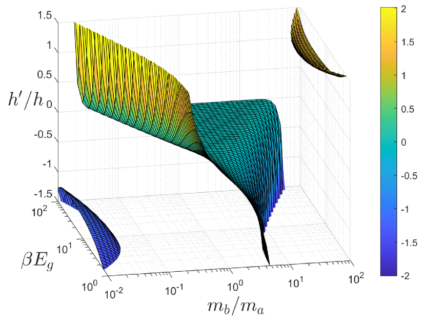
(a)

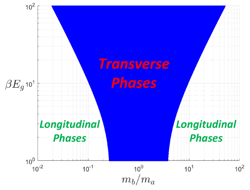
(b)

Figure 3: (a) A ratio between $h^{\prime}$ and $h$ depends on a ratio between the two effective mass ($m_{a}$ and $m_{b}$), temperature, band inversion parameter $E_{g}$ and chemical potential. The ratio $h^{\prime}/h$ is plotted as a function of $m_{b}/m_{a}$, and the band inversion parameter normalized by the temperature. A chemical potential at intersections of the two band is considered. (b) When $|h^{\prime}/h|<1$ ($|h^{\prime}/h|>1$), the classical ground state is transverse (longitudinal) phases. Combining this with Fig. (a), we show the phase diagram as a function of $m_{b}/m_{a}$ and $\beta E_{g}$.

.3 Derivation of classical ground-state phase diagram without Rashba coupling

In this section, we describe the minimization of Eq. (2) of the main text, while we describe the minimization of Eq. (.2) in Sec. .8. Note first that spatial derivative term in Eq. (2) is positive definite, $\lambda|\nabla\vec{\Phi}|^{2}\geq 0$. Thus, only a spatially uniform solution of $\vec{\Phi}$ minimizes the action,

$$\mathcal{L} =A(\Phi^{\prime 2}+\Phi^{\prime\prime 2})+B[\Phi^{\prime 4}+\Phi^{\prime\prime 4}+6\Phi^{\prime 2}\Phi^{\prime\prime 2}]$$

$$-4B\Phi^{\prime 2}\Phi^{\prime\prime 2}(\mathrm{cos}\eta_{1}\mathrm{cos}\eta_{2}\mathrm{cos}\alpha_{1}+\mathrm{sin}\eta_{1}\mathrm{sin}\eta_{2}\mathrm{cos}\alpha_{2})^{2}+2h^{\prime}\Phi^{\prime}\Phi^{\prime\prime}\mathrm{cos}\eta_{1}\mathrm{cos}\eta_{2}\mathrm{sin}\alpha_{1}-2h\Phi^{\prime}\Phi^{\prime\prime}\mathrm{sin}\eta_{1}\mathrm{sin}\eta_{2}\mathrm{sin}\alpha_{2},$$

$$\equiv A(\Phi^{\prime 2}+\Phi^{\prime\prime 2})+B[\Phi^{\prime 4}+\Phi^{\prime\prime 4}+6\Phi^{\prime 2}\Phi^{\prime\prime 2}]-2\Phi^{\prime}\Phi^{\prime\prime}g(\eta_{1},\eta_{2},\alpha_{1},\alpha_{2}),$$ (.3.1)

with $A\equiv-(\alpha-2/g)<0$ and $B=-\gamma>0$. Here $\Phi^{\prime}$ and $\Phi^{\prime\prime}$ are the norm of the four-component vector fields $\vec{\Phi}^{\prime}$ and $\vec{\Phi}^{\prime\prime}$ respectively. $\eta_{1}$, $\eta_{2}$, $\alpha_{1}$ and $\alpha_{2}$ define relative angles among $\vec{\Phi}^{\prime}$, $\vec{\Phi}^{\prime\prime}$ and a $0x$ plane subtended by $\vec{e}_{x}$ and $\vec{e}_{0}$ (Figs. 4(a)–4(d)). $\eta_{1}$ ($\eta_{2}$) is an angle between $\vec{\Phi}^{\prime}$ ($\vec{\Phi}^{\prime\prime}$) and the $0x$ plane (Figs. 4(a), 4(b)). To define $\alpha_{1}$ and $\alpha_{2}$, we decompose $\vec{\Phi}^{\prime}$ and $\vec{\Phi}^{\prime\prime}$ into a component parallel to the $0x$ plane and the other, $\vec{\Phi}^{\prime}=\vec{\Phi}^{\prime}_{0x}+\vec{\Phi}^{\prime}_{yz}$, $\vec{\Phi}^{\prime\prime}=\vec{\Phi}^{\prime\prime}_{0x}+\vec{\Phi}^{\prime\prime}_{yz}$. $\alpha_{1}$ is an angle between $\vec{\Phi}^{\prime}_{0x}$ and $\vec{\Phi}^{\prime\prime}_{0x}$ and $\alpha_{2}$ is an angle between $\vec{\Phi}^{\prime}_{yz}$ and $\vec{\Phi}^{\prime\prime}_{yz}$ (Figs. 4(c), 4(d)).

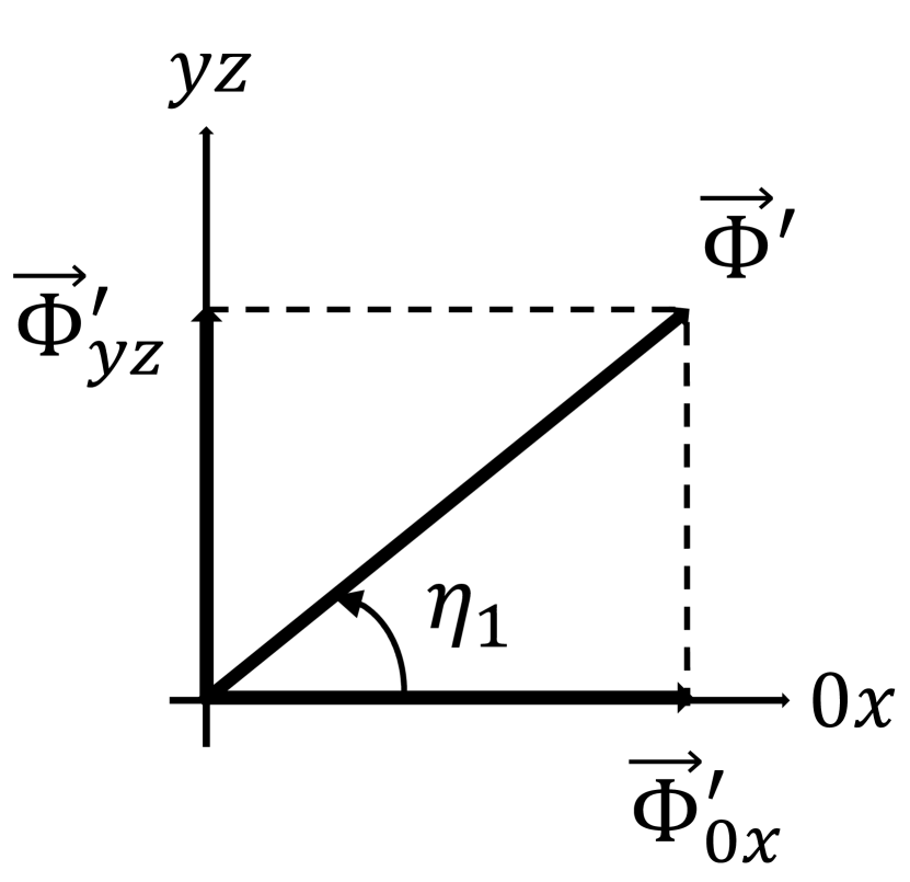
(a)

(c)

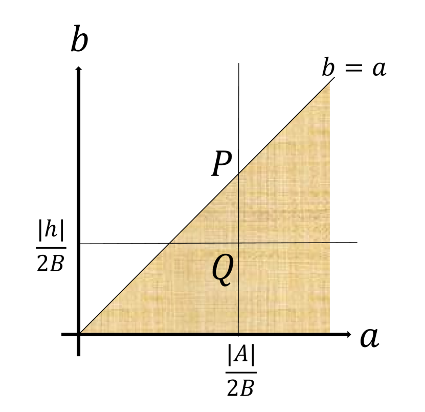
(e)

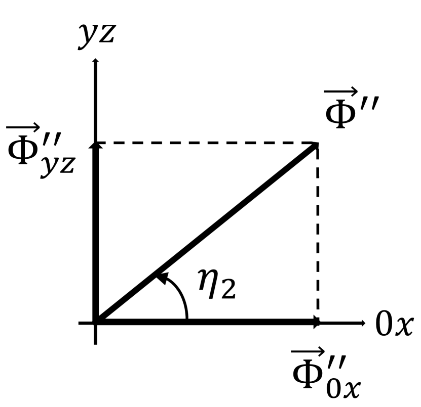
(b)

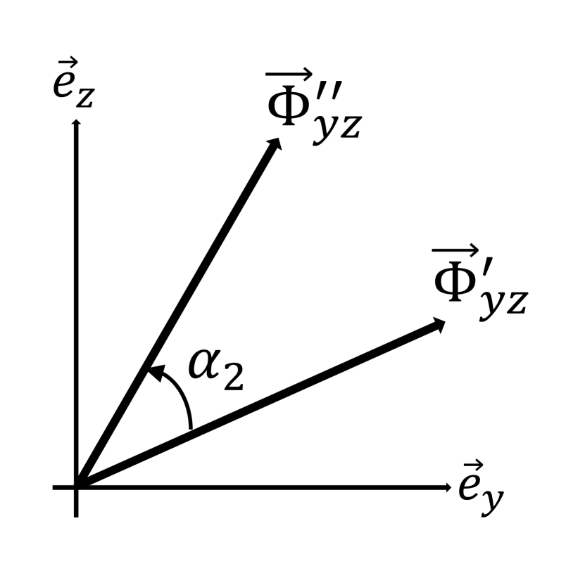
(d)

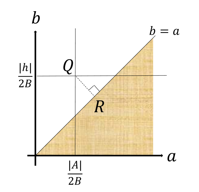
(f)

Figure 4: (a–d) Definitions of $\eta_{1}$, $\eta_{2}$, $\alpha_{1}$ and $\alpha_{2}$. (e, f) Minimization of ${\cal L}_{1}(a)+{\cal L}_{2}(b)$ in a domain of $0\leq b\leq a$. ${\cal L}_{1}(a)$ is minimized along a line of $a=|A|/2B$. ${\cal L}_{2}(b)$ is minimized in a region of $b\geq|h|/2B$. When $|A|>|h|$, ${\cal L}_{1}(a)+{\cal L}_{2}(b)$ is minimized along a finite length of line: $a=|A|/2B$ and $|A|/2B\geq b\geq|h|/2B$ (a line of PQ in Fig. (e)). When $|A|<|h|$, ${\cal L}_{1}(a)+{\cal L}_{2}(b)$ is minimized at a point on the domain boundary: $a=b=\frac{1}{2}(\frac{|h|}{2B}+\frac{|A|}{2B})$ (a point of R in Fig. (f)).

We first minimize the third term of Eq. (.3) that depends on $\eta_{1}$, $\eta_{2}$, $\alpha_{1}$ and $\alpha_{2}$ for fixed $\Phi^{\prime}$ and $\Phi^{\prime\prime}$. Namely, we maximize the following function for fixed $\Phi^{\prime}$ and $\Phi^{\prime\prime}$,

$$g(\eta_{1},\eta_{2},\alpha_{1},\alpha_{2})=2B\Phi^{\prime}\Phi^{\prime\prime}(\mathrm{cos}\eta_{1}\mathrm{cos}\eta_{2}\mathrm{cos}\alpha_{1}+\mathrm{sin}\eta_{1}\mathrm{sin}\eta_{2}\mathrm{cos}\alpha_{2})^{2}-h^{\prime}\mathrm{cos}\eta_{1}\mathrm{cos}\eta_{2}\mathrm{sin}\alpha_{1}+h\mathrm{sin}\eta_{1}\mathrm{sin}\eta_{2}\mathrm{sin}\alpha_{2}.$$ (.3.2)

The function is a sum of quadratic functions of $x\equiv\mathrm{cos}(\eta_{1}-\eta_{2})$ and $y\equiv\mathrm{cos}(\eta_{1}+\eta_{2})$,

$$g=C(\frac{\mathrm{cos}\alpha_{1}+\mathrm{cos}\alpha_{2}}{2}x+\frac{\mathrm{cos}\alpha_{1}-\mathrm{cos}\alpha_{2}}{2}y)^{2}+\frac{h\mathrm{sin}\alpha_{2}-h^{\prime}\mathrm{sin}\alpha_{1}}{2}x-\frac{h\mathrm{sin}\alpha_{2}+h^{\prime}\mathrm{sin}\alpha_{1}}{2}y,$$ (.3.3)

with $C\equiv 2B\Phi^{\prime}\Phi^{\prime\prime}>0$, $\frac{\partial^{2}g}{\partial x^{2}}\geq 0$ and $\frac{\partial^{2}g}{\partial y^{2}}\geq 0$. Since a domain of $x$ and $y$ is bounded by $(x,y)\in[-1,1]\times[-1,1]$, the function takes a maximum value at either one of the four corners of the domain; $(x,y)=\{(-1,-1),(-1,1),(1,-1),(1,1)\}$. By definition, $(\alpha_{1},\alpha_{2},x,y)$ and $(\alpha_{1}+\pi,\alpha_{2}+\pi,-x,-y)$ represent the same vectors. Thus, we take $(x,y)$ at $(1,1)$ or at $(1,-1)$ and maximize $g$ with respect to $\alpha_{1}$ and $\alpha_{2}$. When $x=y=1$, $\eta_{1}=\eta_{2}=0$, and $g=-C\mathrm{sin}^{2}\alpha_{1}-h^{\prime}\mathrm{sin}\alpha_{1}+C$; When $x=-y=1$, $\eta_{1}=\eta_{2}=\frac{\pi}{2}$, and $g=-C\mathrm{sin}^{2}\alpha_{2}+h\mathrm{sin}\alpha_{2}+C$. Such $g$ is maximized with respect to $\alpha_{1}$ and/or $\alpha_{2}$ at the following points,

$$\left\{\begin{array}[]{cllll}\eta_{1}=\eta_{2}=\frac{\pi}{2},&\alpha_{1}\!\ {\rm undefined},&\sin\alpha_{2}=\frac{h}{2C},&g=C+\frac{h^{2}}{4C},&(|h^{\prime}|<|h|<2C),\\ \eta_{1}=\eta_{2}=0,&\sin\alpha_{1}=-\frac{h^{\prime}}{2C},&\alpha_{2}\!\ {\rm undefined},&g=C+\frac{{h^{\prime}}^{2}}{4C},&(|h|<|h^{\prime}|<2C),\\ \eta_{1}=\eta_{2}=\frac{\pi}{2},&\alpha_{1}\!\ {\rm undefined},&\sin\alpha_{2}=\frac{h}{|h|},&g=|h|,&(|h^{\prime}|<|h|,2C<|h|),\\ \eta_{1}=\eta_{2}=0,&\sin\alpha_{1}=-\frac{h^{\prime}}{|h^{\prime}|},&\alpha_{2}\!\ {\rm undefined},&g=|h^{\prime}|,&(|h|<|h^{\prime}|,2C<|h^{\prime}|).\\ \end{array}\right.$$ (.3.8)

Eq. (.3.8) is symmetric with respect to an exchange between $h$ and $-h^{\prime}$ and between $\alpha_{1}$ and $\alpha_{2}$. We consider a case of $|h|>|h^{\prime}|$ first, where $\vec{\Phi}^{\prime}$ and $\vec{\Phi}^{\prime\prime}$ are on a $yz$ plane subtended by $\vec{e}_{y}$ and $\vec{e}_{z}$ ($\eta_{1}=\eta_{2}=\pi/2$) and an angle between $\vec{\Phi}^{\prime}$ and $\vec{\Phi}^{\prime\prime}$ is $\alpha_{2}$ (Figs. 4(a), 4(b), 4(d)). $g$ in Eq. (.3.8) is substituted into Eq. (.3),

$$\left\{\begin{array}[]{lc}{\cal L}=-|A|({\Phi^{\prime}}^{2}+{\Phi^{\prime\prime}}^{2})+B({\Phi^{\prime}}^{2}+{\Phi^{\prime\prime}}^{2})^{2}-\frac{h^{2}}{4B}&(2\Phi^{\prime}\Phi^{\prime\prime}\geq\frac{|h|}{2B}),\\ {\cal L}=-|A|({\Phi^{\prime}}^{2}+{\Phi^{\prime\prime}}^{2})+B({\Phi^{\prime}}^{2}+{\Phi^{\prime\prime}}^{2})^{2}+4B{\Phi^{\prime}}^{2}{\Phi^{\prime\prime}}^{2}-2|h|{\Phi^{\prime}}{\Phi^{\prime\prime}}&(2\Phi^{\prime}\Phi^{\prime\prime}\leq\frac{|h|}{2B}).\\ \end{array}\right.$$ (.3.11)

The Lagrangian in Eq. (.3.11) is further minimized in $\Phi^{\prime}$ and $\Phi^{\prime\prime}$. First, ${\cal L}$ is decomposed into a function of $a\equiv{\Phi^{\prime}}^{2}+{\Phi^{\prime\prime}}^{2}$ and a function of $b\equiv 2\Phi^{\prime}\Phi^{\prime\prime}$, each of which can be separately minimized;

$${\cal L}\equiv{\cal L}_{1}(a)+{\cal L}_{2}(b),\ \ {\cal L}_{1}(a)=-|A|a+Ba^{2},\ \ {\cal L}_{2}(b)=\left\{\begin{array}[]{lc}-\frac{h^{2}}{4B}&(b\geq\frac{|h|}{2B}),\\ Bb^{2}-|h|b&(b\leq\frac{|h|}{2B}).\\ \end{array}\right.$$ (.3.14)

${\cal L}_{1}(a)$ and ${\cal L}_{2}(b)$ take respective minimum at the following point or region,

$$a\equiv{\Phi^{\prime}}^{2}+{\Phi^{\prime\prime}}^{2}=\frac{|A|}{2B},\ \ \ b\equiv 2\Phi^{\prime}\Phi^{\prime\prime}\equiv a\sin 2\theta\geq\frac{|h|}{2B}.$$ (.3.15)

with $(\Phi^{\prime},\Phi^{\prime\prime})\equiv\sqrt{a}(\cos\theta,\sin\theta)$ and $0<\theta<\pi/2$. Noting that a domain of $a$ and $b$ is limited by $0<b<a$ together with $|A|\equiv h_{c}$, $B\equiv|\gamma|$, we complete the minimization of the Lagrangian with a help of Figs. 4(e), 4(f).

Case 1: $h_{c}\geq|h|$ and $|h|>|h^{\prime}|$, the global minimum of the action is achieved on a finite length of a line defined as:

$$a\sin\alpha_{2}\sin 2\theta=\frac{h}{2|\gamma|},\ \ \ a\equiv{\Phi^{\prime}}^{2}+{\Phi^{\prime\prime}}^{2}=\frac{h_{c}}{2|\gamma|},\ \ \ \frac{|h|}{2|\gamma|}\leq b\equiv a\sin 2\theta\leq\frac{h_{c}}{2|\gamma|}.$$ (.3.16)

Case 2: $h_{c}\leq|h|$ and $|h|>|h^{\prime}|$, the global minimum in the domain is achieved at a point on the domain boundary, $a=b=\frac{a+b}{2}=\frac{h_{c}+|h|}{4|\gamma|}$:

$$\sin\alpha_{2}=\frac{h}{|h|},\ \ a\equiv{\Phi^{\prime}}^{2}+{\Phi^{\prime\prime}}^{2}=\frac{h_{c}+|h|}{4|\gamma|},\ \ \theta=\frac{\pi}{4}.$$ (.3.17)

In the case of $|h|<|h^{\prime}|$, $\vec{\Phi}^{\prime}$ and $\vec{\Phi}^{\prime\prime}$ are on the $0x$ plane subtended by $\vec{e}_{0}$ and $\vec{e}_{x}$ ($\eta_{1}=\eta_{2}=0$) and the angle between $\vec{\Phi}^{\prime}$ and $\vec{\Phi}^{\prime\prime}$ is $\alpha_{1}$ (Figs. 4(a), 4(b), 4(c)). Following the same argument, we obtain the the other two cases.

Case 3: $h_{c}\geq|h^{\prime}|$ and $|h|<|h^{\prime}|$, the global minimum of the action is achieved on a finite length of a line given by:

$$a\sin\alpha_{1}\sin 2\theta=-\frac{h^{\prime}}{2|\gamma|},\ \ \ a\equiv{\Phi^{\prime}}^{2}+{\Phi^{\prime\prime}}^{2}=\frac{h_{c}}{2|\gamma|},\ \ \ \frac{|h^{\prime}|}{2|\gamma|}\leq b\equiv a\sin 2\theta\leq\frac{h_{c}}{2|\gamma|}.$$ (.3.18)

Case 4: $h_{c}\leq|h^{\prime}|$ and $|h|<|h^{\prime}|$, the global minimum in the domain is achieved at a point on the domain boundary, $a=b=\frac{a+b}{2}=\frac{h_{c}+|h|}{4|\gamma|}$:

$$\sin\alpha_{1}=-\frac{h^{\prime}}{|h^{\prime}|},\ \ a\equiv{\Phi^{\prime}}^{2}+{\Phi^{\prime\prime}}^{2}=\frac{h_{c}+|h^{\prime}|}{4|\gamma|},\ \ \theta=\frac{\pi}{4}.$$ (.3.19)

To summarize these four cases, we have the following four phases.
For $|h^{\prime}|<|h|<h_{c}$ (regular transverse phase: Case 1 with $\alpha_{2}=\varphi$):

$$\vec{\phi}=\rho\mathrm{cos}\theta(\mathrm{cos}\varphi_{0}\vec{e}_{y}+\mathrm{sin}\varphi_{0}\vec{e}_{z})+\mathrm{i}\rho\mathrm{sin}\theta[\mathrm{cos}(\varphi+\varphi_{0})\vec{e}_{y}+\mathrm{sin}(\varphi+\varphi_{0})\vec{e}_{z}],$$

$$\rho=\sqrt{\frac{h_{c}}{2|\gamma|}},\quad\mathrm{sin}\varphi\mathrm{sin}2\theta=\frac{h}{h_{c}}.$$ (.3.20)

For $|h|<|h^{\prime}|<h_{c}$ (regular longitudinal phase: case 3 with $\alpha_{1}=\varphi$):

$$\vec{\phi}=\rho[-\mathrm{sin}\theta\mathrm{cos}(\varphi+\varphi_{0})\vec{e}_{0}+\mathrm{cos}\theta\mathrm{sin}\varphi_{0}\vec{e}_{x}]+\mathrm{i}\rho[\mathrm{cos}\theta\mathrm{cos}\varphi_{0}\vec{e}_{0}+\mathrm{sin}\theta\mathrm{sin}(\varphi+\varphi_{0})\vec{e}_{x}],$$

$$\rho=\sqrt{\frac{h_{c}}{2|\gamma|}},\quad\mathrm{sin}\varphi\mathrm{sin}2\theta=-\frac{h^{\prime}}{h_{c}}.$$ (.3.21)

For $|h^{\prime}|<|h|$, $h_{c}<|h|$ (saturated transverse phase: case 2 with $\alpha_{2}={\rm sgn}(h)\frac{\pi}{2}$):

$$\vec{\phi}=\rho(\mathrm{cos}\varphi_{0}\vec{e}_{y}+\mathrm{sin}\varphi_{0}\vec{e}_{z})-\mathrm{i}\rho\mathrm{sgn}(h)[\mathrm{sin}\varphi_{0}\vec{e}_{y}-\mathrm{cos}\varphi_{0}\vec{e}_{z}],\quad\rho=\sqrt{\frac{h_{c}+|h|}{8|\gamma|}}.$$ (.3.22)

For $|h|<|h^{\prime}|$, $h_{c}<|h^{\prime}|$ (saturated longitudinal phase: case 4 with $\alpha_{1}=-{\rm sgn}(h^{\prime})\frac{\pi}{2}$):

$$\vec{\phi}=\rho[\mathrm{sgn}(-h^{\prime})\mathrm{sin}\varphi_{0}\vec{e}_{0}+\mathrm{sin}\varphi_{0}\vec{e}_{x}]+\mathrm{i}\rho[\mathrm{cos}\varphi_{0}\vec{e}_{0}+\mathrm{sgn}(-h^{\prime})\mathrm{cos}\varphi_{0}\vec{e}_{x}],\quad\rho=\sqrt{\frac{h_{c}+|h^{\prime}|}{8|\gamma|}}.$$ (.3.23)

From Eqs. (.3–.3.23), we obtain a classical ground-state phase diagram at $D=0$ (Fig. 5(a)).

The phase boundaries at $|h|=|h^{\prime}|$ are of the first order. To be more specific, Eq. (2) in the main text at $h=\pm h^{\prime}$ is invariant under the following SO(2) rotation in the four-component vector space of $\vec{\Phi}\equiv\vec{\Phi}^{\prime}+{\rm i}\vec{\Phi}^{\prime\prime}\equiv(-{\rm i}\phi_{0},\phi_{x},\phi_{y},\phi_{z})$,

$$\left(\begin{array}[]{c}-{\rm i}\phi_{0}\\ \phi_{x}\\ \phi_{y}\\ \phi_{z}\\ \end{array}\right)\rightarrow\left(\begin{array}[]{cccc}\cos\Theta&0&\sin\Theta&0\\ 0&\cos\Theta&0&\mp\sin\Theta\\ -\sin\Theta&0&\cos\Theta&0\\ 0&\pm\sin\Theta&0&\cos\Theta\\ \end{array}\right)\left(\begin{array}[]{c}-{\rm i}\phi_{0}\\ \phi_{x}\\ \phi_{y}\\ \phi_{z}\\ \end{array}\right),$$ (.3.36)

with real-valued U(1) phase $\Theta$. The SO(2) rotation interpolates between the transverse configuration and longitudinal configuration. Thus, the general classical solution at $|h|=|h^{\prime}|$ is given by a linear superposition of the two configurations. The phase boundaries at $|h|=h_{c}$ and at $|h^{\prime}|=h_{c}$ are of the second order.

At $h=h^{\prime}=0$, Eq. (2) in the main text is given only by an amplitude of the complex-valued four-components vector $\vec{\Phi}\equiv\vec{\Phi}^{\prime}+{\rm i}\vec{\Phi}^{\prime\prime}$ ($\rho$), an angle between $\vec{\Phi}^{\prime}$ and $\vec{\Phi}^{\prime\prime}$ ($\varphi$), and an amplitude ratio between $\vec{\Phi}^{\prime}$ and $\vec{\Phi}^{\prime\prime}$ ($\theta$),

$${\cal L}=-h_{c}\rho^{2}+|\gamma|\Big{(}\rho^{4}+\rho^{4}\big{(}\sin 2\theta\sin\varphi\big{)}^{2}\Big{)},$$ (.3.37)

with

$$(|\vec{\Phi}^{\prime}|,|\vec{\Phi}^{\prime\prime}|)\equiv\rho(\cos\theta,\sin\theta),\ \ \vec{\Phi}^{\prime}\cdot\vec{\Phi}^{\prime\prime}\equiv|\vec{\Phi}^{\prime}||\vec{\Phi}^{\prime\prime}|\cos\varphi\equiv\frac{\rho^{2}}{2}\sin 2\theta\cos\varphi.$$ (.3.38)

Here $\vec{\Phi}^{\prime}$ and $\vec{\Phi}^{\prime\prime}$ are real and imginary part of the four-components vector $\vec{\Phi}$ respectively, and they are real-valued four-components vectors. Thus, for $h_{c}>0$, the classical solution at $h=h^{\prime}=0$ is given by

$$\rho^{2}=\frac{h_{c}}{2|\gamma|}\ \cap\ \sin 2\theta\sin\varphi=0,$$ (.3.39)

or equivalently,

$$\vec{\Phi}=\rho\vec{n}e^{{\rm i}\theta},$$ (.3.40)

with an arbitrary phase $\theta$ and an arbitrary 4-components real-valued unit vector $\vec{n}$.

As the exchange fields $H_{a}$ and $H_{b}$ are supposed to be small, in the main text (Eqs. (3–5)) we focus on the regular transverse phase and the regular longitudinal phase.

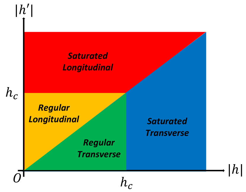
(a)

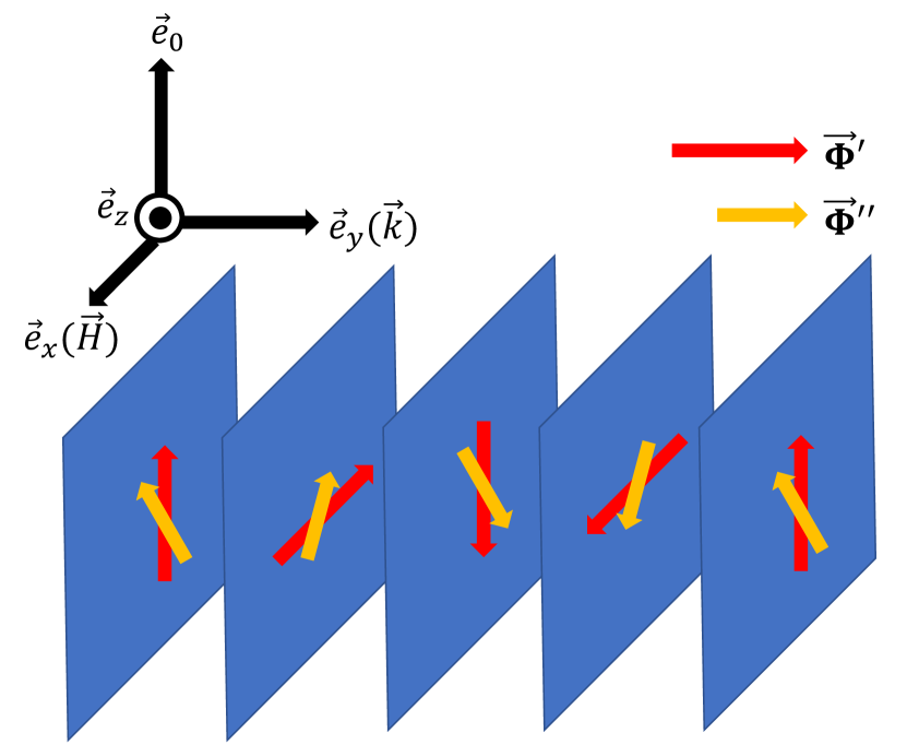
(b)

Figure 5: (a) Classical ground-state phase diagram of the EHDL excitons under magnetic exchange fields without Rashba coupling. The phase diagram remains unchanged with Rashba coupling, except the transverse/longitudinal phases are substituted by corresponding helicoidal/helical phases. (b) A schematic picture of the helical structure of condensed excitons. The real ($\vec{\Phi}^{\prime}$) and imaginary ($\vec{\Phi}^{\prime\prime}$) parts are depicted by red and yellow arrows respectively. The propagation direction $\vec{k}(\vec{e}_{y})$ is along the the in-plane direction perpendicular to the magnetic field, and $\vec{\Phi}^{\prime}$ and $\vec{\Phi}^{\prime\prime}$ rotate in the plane (depicted by blue planes) subtended by a direction of spin singlet ($\vec{e}_{0}$) and a direction of magnetic field $\vec{H}(\vec{e}_{x})$. An angle between $\vec{\Phi}^{\prime}$ and $\vec{\Phi}^{\prime\prime}$ is acute for the regular helical phase. The angle becomes $0$ for $h^{\prime}=0$ and $\pi/2$ for $|h^{\prime}|\geq|h|$ (saturated helical phase). The length of $\vec{\Phi}^{\prime}$ and that of $\vec{\Phi}^{\prime\prime}$ become identical to each other for the saturated helical phase.

.4 Spin rotational symmetry of the excitonic condensate system

In this section, we clarify what continuous spin-rotational symmetry is broken in the transverse and longitudinal phases, i.e. Eq. (6) in the main text. Let us begin with the longitudinal phase:

$$\vec{\phi}_{\parallel}(\theta,\varphi,\varphi_{0})\cdot\vec{\bm{\sigma}}\equiv-\rho\mathrm{sin}\theta[\bm{\sigma}_{0}\mathrm{cos}(\varphi+\varphi_{0})-\mathrm{i}\bm{\sigma}_{x}\mathrm{sin}(\varphi+\varphi_{0})]+\mathrm{i}\rho\mathrm{cos}\theta[\bm{\sigma}_{0}\mathrm{cos}\varphi_{0}-\mathrm{i}\bm{\sigma}_{x}\mathrm{sin}\varphi_{0}]$$

$$= -\rho\mathrm{sin}\theta\mathrm{e}^{-\mathrm{i}(\varphi+\varphi_{0})\bm{\sigma}_{x}}+\mathrm{i}\rho\mathrm{cos}\theta\mathrm{e}^{-\mathrm{i}\varphi_{0}\bm{\sigma_{x}}}=[-\rho\mathrm{sin}\theta\mathrm{e}^{-\mathrm{i}\varphi\bm{\sigma}_{x}}+\mathrm{i}\rho\mathrm{cos}\theta]\mathrm{e}^{-\mathrm{i}\varphi_{0}\bm{\sigma_{x}}}=\vec{\phi}_{\parallel}(\theta,\varphi,0)\cdot\vec{\bm{\sigma}}\!\ \mathrm{e}^{-\mathrm{i}\varphi_{0}\bm{\sigma_{x}}}.$$ (.4.1)

A change of $\varphi_{0}$ by $\delta\varphi_{0}$ in Eq. (.4) leads to a pseudospin rotation of the four-component excitonic pseudospin vector $\vec{\Phi}\equiv\vec{\Phi}^{\prime}+{\rm i}\vec{\Phi}^{\prime\prime}\equiv(-{\rm i}\phi_{0},\phi_{x},\phi_{y},\phi_{z})$. The rotation is within the $0x$ plane subtended by $\vec{e}_{0}$ (singlet component) and $\vec{e}_{x}$ ($x$-component of the triplet pairing field);

$$\left(\begin{array}[]{c}-{\rm i}\phi_{0}\\ \phi_{x}\\ \phi_{y}\\ \phi_{z}\\ \end{array}\right)_{|\varphi_{0}+\delta\varphi_{0}}=\left(\begin{array}[]{cccc}\cos\delta\varphi_{0}&-\sin\delta\varphi_{0}&&\\ \sin\delta\varphi_{0}&\cos\delta\varphi_{0}&&\\ &&1&0\\ &&0&1\\ \end{array}\right)\left(\begin{array}[]{c}-{\rm i}\phi_{0}\\ \phi_{x}\\ \phi_{y}\\ \phi_{z}\\ \end{array}\right)_{|\varphi_{0}}.$$ (.4.14)

The pseudospin rotation within the $0x$ plane can be absorbed by spin rotations around the $x$ axis in the electron and hole layers through a mean-field coupling term,

$$\vec{\phi}_{\parallel}(\varphi_{0}+\delta\varphi_{0})\cdot\bm{a}^{\dagger}\vec{\bm{\sigma}}\bm{b}=\vec{\phi}_{\parallel}(\varphi_{0})\cdot\bm{a}^{\dagger}\vec{\bm{\sigma}}\mathrm{e}^{-\mathrm{i}\delta\varphi_{0}\bm{\sigma_{x}}}\bm{b}=\vec{\phi}_{\parallel}(\varphi_{0})\cdot\bm{a}^{\dagger}\mathrm{e}^{-\mathrm{i}\delta\varphi_{0}\bm{\sigma_{x}}}\vec{\bm{\sigma}}\bm{b}.$$ (.4.15)

Namely, the mean-field term $\vec{\phi}_{\parallel}\cdot{\bm{a}}^{\dagger}\vec{\bm{\sigma}}{\bm{b}}$ is invariant under the followings;

$$\bm{a}\rightarrow\mathrm{e}^{\mathrm{i}\varphi_{a}{\bm{\sigma}}_{x}}\bm{a},\quad\bm{b}\rightarrow\mathrm{e}^{\mathrm{i}\varphi_{b}{\bm{\sigma}}_{x}}\bm{b},\quad\vec{\phi}_{\parallel}(\varphi_{0})\rightarrow\vec{\phi}_{\parallel}(\varphi_{0}+\varphi_{b}-\varphi_{a}).$$ (.4.16)

Similarly, the transverse phase is given by the following classical configuration:

$$\vec{\phi}_{\perp}(\theta,\varphi,\varphi_{0})\cdot\vec{\bm{\sigma}}\equiv\rho\cos\theta{\bm{\sigma}}_{y}e^{{\rm i}\varphi_{0}{\bm{\sigma}}_{x}}+{\rm i}\rho\sin\theta{\bm{\sigma}}_{y}e^{{\rm i}(\varphi+\varphi_{0}){\bm{\sigma}}_{x}}$$

$$=\vec{\phi}_{\perp}(\theta,\varphi,0)\cdot\vec{\bm{\sigma}}\!\ \mathrm{e}^{\mathrm{i}\varphi_{0}\bm{\sigma_{x}}}=\mathrm{e}^{-\mathrm{i}\varphi_{0}\bm{\sigma_{x}}}\!\ \vec{\phi}_{\perp}(\theta,\varphi,0)\cdot\vec{\bm{\sigma}}.$$ (.4.17)

A variation of $\varphi_{0}$ by $\delta\varphi_{0}$ in Eq. (.4) leads to a pseudospin rotation of $\vec{\Phi}\equiv(-{\rm i}\phi_{0},\phi_{x},\phi_{y},\phi_{z})$ within the $yz$ plane subtended by $\vec{e}_{y}$ ($y$-component of the triplet pairing field) and $\vec{e}_{z}$ ($z$-component of the triplet pairing field);

$$\left(\begin{array}[]{c}-{\rm i}\phi_{0}\\ \phi_{x}\\ \phi_{y}\\ \phi_{z}\\ \end{array}\right)_{|\varphi_{0}+\delta\varphi_{0}}=\left(\begin{array}[]{cccc}1&0&&\\ 0&1&&\\ &&\cos\delta\varphi_{0}&-\sin\delta\varphi_{0}\\ &&\sin\delta\varphi_{0}&\cos\delta\varphi_{0}\\ \end{array}\right)\left(\begin{array}[]{c}-{\rm i}\phi_{0}\\ \phi_{x}\\ \phi_{y}\\ \phi_{z}\\ \end{array}\right)_{|\varphi_{0}}.$$ (.4.30)

The pseudospin rotation within the $yz$ plane transforms the mean-field coupling term as

$$\vec{\phi}_{\perp}(\varphi_{0}+\delta\varphi_{0})\cdot\bm{a}^{\dagger}\vec{\bm{\sigma}}\bm{b}=\vec{\phi}_{\perp}(\varphi_{0})\cdot\bm{a}^{\dagger}\vec{\bm{\sigma}}\mathrm{e}^{\mathrm{i}\delta\varphi_{0}\bm{\sigma_{x}}}\bm{b}=\vec{\phi}_{\perp}(\varphi_{0})\cdot\bm{a}^{\dagger}\mathrm{e}^{-\mathrm{i}\delta\varphi_{0}\bm{\sigma_{x}}}\vec{\bm{\sigma}}\bm{b}.$$ (.4.31)

The variation can be absorbed by the following spin rotations around the $x$ axis in the electron and hole layers,

$$\bm{a}\rightarrow\mathrm{e}^{\mathrm{i}\varphi_{a}{\bm{\sigma}}_{x}}\bm{a},\quad\bm{b}\rightarrow\mathrm{e}^{\mathrm{i}\varphi_{b}{\bm{\sigma}}_{x}}\bm{b},\quad\vec{\phi}_{\perp}(\varphi_{0})\rightarrow\vec{\phi}_{\perp}(\varphi_{0}-\varphi_{b}-\varphi_{a}).$$ (.4.32)

Eqs. (.4.16, .4.32) are equivalent to Eq. (6) in the main text.

.5 Relation between the Goldstone modes and the $U(1)$ gauge symmetry

In the main text, the transverse configuration and longitudinal configuration are described by three phase variables, $\theta$, $\varphi$ and $\varphi_{0}$. As shown in Sec. .4, $\varphi_{0}$ is a rotational angle of the spin rotation of the four-component exciton’s pseudospin vector $\vec{\Phi}\equiv\vec{\Phi}^{\prime}+{\rm i}\vec{\Phi}^{\prime\prime}\equiv(-{\rm i}\phi_{0},\phi_{x},\phi_{y},\phi_{z})$. On the other hand, $\theta$ and $\varphi$ define an amplitude ratio between $\vec{\Phi}^{\prime}$ and $\vec{\Phi}^{\prime\prime}$ and an angle between $\vec{\Phi}^{\prime}$ and $\vec{\Phi}^{\prime\prime}$:

$$\big{(}|\vec{\Phi}^{\prime}|,|\vec{\Phi}^{\prime\prime}|\big{)}\equiv\rho(\cos\theta,\sin\theta),\ \ \vec{\Phi}^{\prime}\cdot\vec{\Phi}^{\prime\prime}=|\vec{\Phi}^{\prime}||\vec{\Phi}^{\prime\prime}|\cos\varphi.$$ (.5.1)

Here $\vec{\Phi}^{\prime}$ and $\vec{\Phi}^{\prime\prime}$ are real and imaginary parts of $\vec{\Phi}\equiv(-{\rm i}\phi_{0},\phi_{x},\phi_{y},\phi_{z})$ respectively, and they are four-component real-valued vectors. Roughly speaking, a combination of $\varphi$ (angle) and $\theta$ (amplitude ratio) can be regarded as the relative U(1) phase degree of freedom between the two layers. To show this, consider the U(1) gauge transformations in the two layers, that induces a U(1) gauge transformation of the excitonic order parameters $\vec{\Phi}\equiv\vec{\Phi}^{\prime}+{\rm i}\vec{\Phi}^{\prime\prime}$,

$${\bm{a}}\rightarrow e^{{\rm i}\frac{\psi}{2}}{\bm{a}},\ \ {\bm{b}}\rightarrow e^{-{\rm i}\frac{\psi}{2}}{\bm{b}},$$

$$\vec{\Phi}\rightarrow e^{{\rm i}\psi}\!\ \vec{\Phi},\ \ \ \vec{\Phi}^{\prime}\rightarrow\cos\psi\!\ \vec{\Phi}^{\prime}-\sin\psi\!\ \vec{\Phi}^{\prime\prime},\ \ \vec{\Phi}^{\prime\prime}\rightarrow\sin\psi\!\ \vec{\Phi}^{\prime}+\cos\psi\!\ \vec{\Phi}^{\prime\prime}.$$ (.5.2)

Under the transformation, the angle and amplitude ratio are transformed as follows,

$$\left(\begin{array}[]{c}|\vec{\Phi}^{\prime}|^{2}-|\vec{\Phi}^{\prime\prime}|^{2}\\ 2\vec{\Phi}^{\prime}\cdot\vec{\Phi}^{\prime\prime}\\ \end{array}\right)\equiv\rho^{2}\left(\begin{array}[]{c}\cos 2\theta\\ \sin 2\theta\cos\varphi\\ \end{array}\right)\rightarrow\rho^{2}\left(\begin{array}[]{cc}\cos 2\psi&-\sin 2\psi\\ \sin 2\psi&\cos 2\psi\\ \end{array}\right)\left(\begin{array}[]{c}\cos 2\theta\\ \sin 2\theta\cos\varphi\\ \end{array}\right).$$ (.5.11)

This suggests that $\sin 2\theta\sin\varphi$ is invariant under the relative U(1) gauge transformation, and a simultaneous change of the angle ($\varphi$) and the amplitude ratio ($\theta$) along a loop of $\sin 2\theta\sin\varphi\!\ =$ constant can be regarded as the relative U(1) phase degree of freedom between the two layers. To be more precise, the relative U(1) gauge transformation not only induces the change of the angle ($\varphi$) and the amplitude ratio ($\theta$), but also induces a pseudospin rotation of the four-component excitonic pseudospin vector $\vec{\Phi}$ ($\varphi_{0}$).

To see this, let us show that the relative U(1) gauge transformation can be absorbed into a combination of changes of $\theta$, $\varphi$ and $\varphi_{0}$ that satisfies the constraint Eq. (5);

$$\left\{\begin{array}[]{l}e^{i\psi}\vec{\phi}_{\lambda}(\theta,\varphi,\varphi_{0})=\vec{\phi}_{\lambda}(\theta(\psi),\varphi(\psi),\varphi_{0}(\psi)),\\ \sin 2\theta(\psi)\sin\varphi(\psi)=\sin 2\theta\sin\varphi={\sf{h}}\equiv\left\{\begin{array}[]{cc}\frac{h}{h_{c}}&(\lambda=\perp),\\ -\frac{h^{\prime}}{h_{c}}&(\lambda=\parallel),\\ \end{array}\right.\\ \end{array}\right.$$ (.5.16)

for both the transverse phase ($\lambda=\perp$) and the longitudinal phase ($\lambda=\parallel$). When there is the Rashba coupling, we can generalize the argument into the helical and helicoidal phase by replacing $\varphi_{0}$ by $\varphi_{0}-Ky$ (see Sec. .8). In the following, we only sketch the argument for the transverse phase, while the argument for the longitudinal phase goes as well. Without loss of generality, we take $\varphi_{0}$ to be $-\varphi$ in Eq. (3) of the main text and apply the gauge transformation on Eq. (3) as,

$$\vec{\phi}_{\perp}(\theta,\varphi,\varphi_{0}) =\rho(\mathrm{cos}\theta\mathrm{cos}\varphi+\mathrm{i}\mathrm{sin}\theta)\vec{e}_{y}-\rho\mathrm{cos}\theta\mathrm{sin}\varphi\vec{e}_{z},$$ (.5.17)

$$e^{i\psi}\vec{\phi}_{\perp}(\theta,\varphi,\varphi_{0}) =\rho(\mathrm{cos}\theta\mathrm{cos}\varphi\mathrm{cos}\psi-\mathrm{sin}\theta\mathrm{sin}\psi)\vec{e}_{y}+\mathrm{i}\rho(\mathrm{sin}\theta\mathrm{cos}\psi+\mathrm{cos}\theta\mathrm{cos}\varphi\mathrm{sin}\psi)\vec{e}_{y}$$

$$-\rho\mathrm{cos}\theta\mathrm{sin}\varphi\mathrm{cos}\psi\vec{e}_{z}-\mathrm{i}\rho\mathrm{cos}\theta\mathrm{sin}\varphi\mathrm{sin}\psi\vec{e}_{z}.$$ (.5.18)

In terms of $\theta^{\prime}$, $\varphi^{\prime}$, $\varphi^{\prime}_{0}$ ($\varphi^{\prime\prime}_{0}\equiv\varphi^{\prime}+\varphi^{\prime}_{0}$), Eq. (.5.18) is equated to

$$\vec{\phi}_{\perp}(\theta^{\prime},\varphi^{\prime},\varphi^{\prime}_{0})=\rho\mathrm{cos}\theta^{\prime}\mathrm{cos}(\varphi^{\prime}-\varphi^{\prime\prime}_{0})\vec{e}_{y}+\mathrm{i}\rho\mathrm{sin}\theta^{\prime}\mathrm{cos}\varphi^{\prime\prime}_{0}\vec{e}_{y}-\rho\mathrm{cos}\theta^{\prime}\mathrm{sin}(\varphi^{\prime}-\varphi^{\prime\prime}_{0})\vec{e}_{z}+\mathrm{i}\rho\mathrm{sin}\theta^{\prime}\mathrm{sin}\varphi^{\prime\prime}_{0}\vec{e}_{z}.$$ (.5.19)

The comparison of (.5.19) with (.5.18) gives four equations:

$$\mathrm{cos}\theta^{\prime}\mathrm{cos}(\varphi^{\prime}-\varphi^{\prime\prime}_{0})=\mathrm{cos}\theta\mathrm{cos}\varphi\mathrm{cos}\psi-\mathrm{sin}\theta\mathrm{sin}\psi,$$ (.5.20)

$$\mathrm{sin}\theta^{\prime}\mathrm{cos}\varphi^{\prime\prime}_{0}=\mathrm{sin}\theta\mathrm{cos}\psi+\mathrm{cos}\theta\mathrm{cos}\varphi\mathrm{sin}\psi,$$ (.5.21)

$$\mathrm{cos}\theta^{\prime}\mathrm{sin}(\varphi^{\prime}-\varphi^{\prime\prime}_{0})=\mathrm{cos}\theta\mathrm{sin}\varphi\mathrm{cos}\psi,$$ (.5.22)

$$-\mathrm{sin}\theta^{\prime}\mathrm{sin}\varphi^{\prime\prime}_{0}=\mathrm{cos}\theta\mathrm{sin}\varphi\mathrm{sin}\psi.$$ (.5.23)

Note first that $\mathrm{(\ref{eqn4-4})}^{2}+\mathrm{(\ref{eqn4-5})}^{2}+\mathrm{(\ref{eqn4-6})}^{2}+\mathrm{(\ref{eqn4-7})}^{2}$ are trivially satisfied, so that Eqs. (.5.20–.5.23) have only three independent equations. Three unknown variables $(\theta^{\prime},\varphi^{\prime},\varphi^{\prime}_{0})$ can be solved in favor for $(\theta,\varphi,\varphi_{0}=-\varphi)$ and $\psi$.

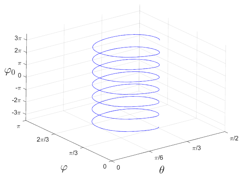
(a)

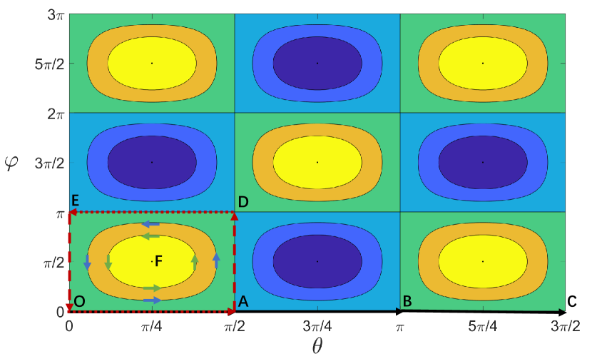
(b)

Figure 6: (a) A parameter plot of $(\theta(\psi)$, $\varphi(\psi)$, $\varphi_{0}(\psi))$ where the initial point $(\theta(0)$, $\varphi(0)$, $\varphi_{0}(0))$ satisfy ${\sf{h}}=\sin 2\theta(0)\sin\varphi(0)=0.75$, $\sin\varphi(0)=0.8$, and $\varphi_{0}(0)=0$. When $\psi$ increases by $\pi$, $\varphi$ decreases by $\pi$, while $(\theta,\varphi)$ goes along a closed curve ($\tilde{h}\equiv\sin 2\theta\sin\varphi=\sf{h}$) at one time. (b) The contour plot of $\tilde{h}={\sf{h}}$ for different values of ${\sf{h}}$. When ${\sf{h}}=1$, the projection becomes a point (F). When ${\sf{h}}=0$, the projection tends to a rectangule (O$\rightarrow$ A $\rightarrow$ D $\rightarrow$ E $\rightarrow$ O), but it is also equivalent to go along a straight line (O$\rightarrow$ A $\rightarrow$ B $\rightarrow$ C $\rightarrow$ O), as different values of $(\psi,\theta,\varphi,\varphi_{0})$ may be equivalent in the special case of $\tilde{h}=0$.

From Eqs. (.5.21, .5.23), we get:

$$-\mathrm{tan}\varphi^{\prime\prime}_{0}=\frac{\mathrm{cos}\theta\mathrm{sin}\varphi\mathrm{sin}\psi}{\mathrm{sin}\theta\mathrm{cos}\psi+\mathrm{cos}\theta\mathrm{cos}\varphi\mathrm{sin}\psi},$$ (.5.24)

From Eqs. (.5.20, .5.22), we get:

$$\mathrm{tan}(\varphi^{\prime}-\varphi^{\prime\prime}_{0})=\frac{\mathrm{cos}\theta\mathrm{sin}\varphi\mathrm{cos}\psi}{\mathrm{cos}\theta\mathrm{cos}\varphi\mathrm{cos}\psi-\mathrm{sin}\theta\mathrm{sin}\psi},$$ (.5.25)

Using Eqs. (.5.24, .5.25) together with $\sin 2\theta\sin\varphi={\sf{h}}$, we have

$$\mathrm{tan}\varphi^{\prime}=\frac{\mathrm{tan}(\varphi^{\prime}-\varphi^{\prime\prime}_{0})+\mathrm{tan}\varphi^{\prime\prime}_{0}}{1-\mathrm{tan}(\varphi^{\prime}-\varphi^{\prime\prime}_{0})\mathrm{tan}\varphi^{\prime\prime}_{0}}=\frac{{\sf{h}}}{\mathrm{sin}2\theta\mathrm{cos}\varphi\mathrm{cos}2\psi+\mathrm{cos}2\theta\mathrm{sin}2\psi}.$$ (.5.26)

From Eqs. (.5.20, .5.22), we get:

$$\mathrm{cos}^{2}\theta^{\prime}=\frac{1}{2}(1+\mathrm{cos}2\theta\mathrm{cos}2\psi-\mathrm{sin}2\theta\mathrm{sin}2\psi\mathrm{cos}\varphi),$$ (.5.27)

From Eqs. (.5.21, .5.23), we get:

$$\mathrm{sin}^{2}\theta^{\prime}=\frac{1}{2}(1-\mathrm{cos}2\theta\mathrm{cos}2\psi+\mathrm{sin}2\theta\mathrm{sin}2\psi\mathrm{cos}\varphi).$$ (.5.28)

Eqs. (.5.24, .5.26–.5.28) are nothing but the solutions of $\theta^{\prime}$, $\varphi^{\prime}$, $\varphi^{\prime}_{0}$ in favor for $\theta$, $\varphi$, $\varphi_{0}=-\varphi$ and $\psi$. To see that such $\theta^{\prime}$ and $\varphi^{\prime}$ satisfy the same condition as $\theta$ and $\varphi$, i.e. $\sin 2\theta^{\prime}\sin\varphi^{\prime}={\sf{h}}$, we multiply Eq. (.5.27) by Eq. (.5.28), to have

$$\mathrm{sin}^{2}2\theta^{\prime}=4\mathrm{sin}^{2}\theta^{\prime}\mathrm{cos}^{2}\theta^{\prime}=1-(\mathrm{cos}2\theta\mathrm{cos}2\psi-\mathrm{sin}2\theta\mathrm{sin}2\psi\mathrm{cos}\varphi)^{2},$$ (.5.29)

and we square Eq. (.5.26), to have

$$\mathrm{sin}^{2}\varphi^{\prime}=\frac{\mathrm{tan}^{2}\varphi^{\prime}}{1+\mathrm{tan}^{2}\varphi^{\prime}}=\frac{{\sf{h}}^{2}}{(\mathrm{sin}2\theta\mathrm{cos}\varphi\mathrm{cos}2\psi+\mathrm{cos}2\theta\mathrm{sin}2\psi)^{2}+{\sf{h}}^{2}}.$$ (.5.30)

Combining these two, we get:

$$\mathrm{sin}^{2}2\theta^{\prime}\mathrm{sin}^{2}\varphi^{\prime}={\sf{h}}^{2}\frac{1-(\mathrm{cos}2\theta\mathrm{cos}2\psi-\mathrm{sin}2\theta\mathrm{sin}2\psi\mathrm{cos}\varphi)^{2}}{(\mathrm{sin}2\theta\mathrm{cos}\varphi\mathrm{cos}2\psi+\mathrm{cos}2\theta\mathrm{sin}2\psi)^{2}+{\sf{h}}^{2}}={\sf{h}}^{2}.$$ (.5.31)

Because $\theta^{\prime}$ and $\varphi^{\prime}$ can be regarded as smooth functions of $\psi$ that reduce to $\theta$ and $\varphi$ at $\psi=0$ respectively, we can conclude that $\mathrm{sin}2\theta^{\prime}\mathrm{sin}\varphi^{\prime}={\sf{h}}$. This completes the proof of Eq. (.5.16) for the transverse phase. In other words, the gapless Goldstone mode associated with the symmetry breaking of the relative gauge symmetry is given by a combination of the $\varphi_{0}$ mode and a variation of $\theta$ and $\varphi$ within the constraint of Eq. (5) in the main text.

A parameter-plot of $(\theta(\psi),\varphi(\psi),\varphi_{0}(\psi))$ is given in Fig. 6(a) for a given $(\theta(0),\varphi(0),\varphi_{0}(0))$. The plot takes a form of a helical curve in the $(\theta,\varphi,\varphi_{0})$ space. A projection of the curve onto the $(\theta,\varphi)$ plane is a circle that is defined by $\tilde{h}\equiv\sin 2\theta\sin\varphi={\sf{h}}$. When $\psi$ changes by $\pi$, $(\theta,\varphi)$ goes around the circle once and $\varphi_{0}$ changes by $-\pi$. When ${\sf{h}}=1\!\ (h=h_{c})$, the circle reduces to a point of $\theta=\pi/4+n\pi/2$ and $\varphi=\pi/2+n\pi$, and the helical curve reduces to a straight line of $\psi=-\varphi_{0}$. When ${\sf{h}}=0$, the parameter plot of $(\theta(\psi),\varphi(\psi),\varphi_{0}(\psi))$ still preserves the periodicity in a trickly way. To see this, we take an initial point at $\psi=0$ as $(\theta,\varphi,\varphi_{0})=(0,0,0)$. When $\psi$ changes from $0$ to $\pi/{2}$, $(\theta(\psi),\varphi(\psi),\varphi_{0}(\psi))=(\psi,0,0)$. At $\psi=\pi/2$, $\varphi(\psi)$ jumps from $0$ to $\pi$. When $\psi$ changes from $\pi/2$ to $\pi$, $(\theta(\psi),\varphi(\psi),\varphi_{0}(\psi))=(\pi-\psi,\pi,0)$. At $\psi=\pi$, $\varphi(\psi)$ jumps from $\pi$ to $0$, and $\varphi_{0}(\psi)$ jumps from $0$ to $-\pi$. Thus, the periodicity is still true: when $\psi$ changes by $\pi$, $\varphi_{0}$ changes by $-\pi$, and $(\theta,\varphi)$ comes back to the same point.

.6 Derivation of the spin-charge coupled Josephson equations without Rashba coupling

In this section, we derive the spin-charge coupled Josephson equation for the transverse and longitudinal phases. In the main text, we introduced a quantum-dot junction model (Eqs. (10–12)). Applying local (time-dependent) gauge transformations in the electron and hole layers, we obtain

$$\mathcal{S}_{\rm mf}=\int d\tau\sum_{j=1,2}\sum_{\alpha}\Big{\{}{\bm{a}}^{\dagger}_{j\alpha}\big{[}\partial_{\tau}+{\bm{H}}_{a\alpha}-\mu\big{]}{\bm{a}}_{j\alpha}+{\bm{b}}^{\dagger}_{j\alpha}\big{[}\partial_{\tau}+{\bm{H}}_{b\alpha}-\mu-\frac{\eta_{j}}{2}\big{(}V_{C}+V_{S}{\bm{\sigma}}_{x}\big{)}\big{]}{\bm{b}}_{j\alpha}-\vec{\phi}_{\omega}(\psi_{j},\varphi_{0j})\cdot{\bm{a}}^{\dagger}_{j\alpha}\vec{\bm{\sigma}}{\bm{b}}_{j\alpha}+{\rm h.c.}\Big{\}}$$ (.6.1)

with $\omega=\perp,\parallel$ and $\eta_{1}=-\eta_{2}=1$. Here $V_{C}$ is charge voltage difference between the electron and hole layers respectively, while $V_{S}$ is the sum of (difference between) the spin voltage in the electron layer and the spin voltage in the hole layer for the transverse (longitudinal) phase;

$$V_{C}=V_{Cb}-V_{Ca},\quad V_{S}=V_{Sb}\pm V_{Sa}.$$ (.6.2)

Namely, “$+$” is for transverse $(\omega=\perp)$ and “$-$” for longitudinal $(\omega=\parallel)$. Note that we treat $V_{C}$ and $V_{S}$ as external fields. The excitonic mean fields in the two regions are identical to each other except for the two gapless U(1) phase variables;

$$\vec{\phi}_{\omega}(\psi_{j},\varphi_{0j})\cdot\vec{\bm{\sigma}}=\vec{\phi}_{\omega}(\psi=0,\varphi_{0}=0)\cdot\vec{\bm{\sigma}}\mathrm{e}^{{\rm i}\psi_{j}\pm{\rm i}\varphi_{0j}{\bm{\sigma}}_{x}}$$ (.6.3)

with $\pm$ for $\omega=yz,0x$ respectively. Note that $V_{C}$, $V_{S}$, and $\vec{\phi}_{\omega}(\psi=0,\varphi_{0}=0)\equiv\vec{\phi}_{\omega}$ are treated as given (e.g. external) static variables, and the gapless U(1) phase variables, $\psi_{j}$ and $\varphi_{0j}$ $(j=1,2)$, are treated as dynamical variables. In terms of a global gauge transformation in the hole layer, $\mathrm{e}^{{\rm i}\psi_{j}\pm{\rm i}\varphi_{0j}{\bm{\sigma}}_{x}}{\bm{b}}_{j\alpha}\rightarrow{\bm{b}}_{j\alpha}$, the dependence on the gapless phase variables can be removed from the mean field coupling. After the transformation, the phase variables appear in the tunneling part $S_{T}$; accordingly, we have

$$\mathcal{S}[\bm{\Psi},\bm{\Psi}^{\dagger},\psi_{j},\varphi_{0j};V_{C},V_{S}]\equiv\mathcal{S}_{\rm mf}[\bm{\Psi},\bm{\Psi}^{\dagger},\psi_{j},\varphi_{0j};V_{C},V_{S}]+\mathcal{S}_{T}[\bm{\Psi},\bm{\Psi}^{\dagger},\psi_{j},\varphi_{0j}]=\int\mathrm{d}\tau\sum_{\alpha\beta}\bm{\Psi}_{\alpha}^{\dagger}(\bm{\mathcal{G}}^{-1})_{\alpha\beta}\bm{\Psi}_{\beta},$$ (.6.4)

$$(\bm{\mathcal{G}}^{-1})_{\alpha\beta}=\left(\begin{array}[]{cccc}\bm{G}^{-1}_{a\alpha}\delta_{\alpha\beta}&-\vec{\phi}_{\omega}\cdot\vec{\bm{\sigma}}\delta_{\alpha\beta}&T^{(a)}_{\alpha\beta}&0\\ -\vec{\phi}_{\omega}^{*}\cdot\vec{\bm{\sigma}}\delta_{\alpha\beta}&({\bm{G}}^{-1}_{b\alpha}+{\bm{\Delta}}_{1})\delta_{\alpha\beta}&0&T^{(b)}_{\alpha\beta}\mathrm{e}^{\mathrm{i}(\tilde{\psi}\pm\tilde{\varphi}_{0}\bm{\sigma}_{x})}\\ T_{\beta\alpha}^{(a)*}&0&{\bm{G}}^{-1}_{a\alpha}\delta_{\alpha\beta}&-\vec{\phi}_{\omega}\cdot\vec{\bm{\sigma}}\delta_{\alpha\beta}\\ 0&T_{\beta\alpha}^{(b)*}\mathrm{e}^{-\mathrm{i}(\tilde{\psi}\pm\tilde{\varphi}_{0}\bm{\sigma}_{x})}&-\vec{\phi}_{\omega}^{*}\cdot\vec{\bm{\sigma}}\delta_{\alpha\beta}&({\bm{G}}^{-1}_{b\alpha}+{\bm{\Delta}}_{2})\delta_{\alpha\beta}\end{array}\right),$$ (.6.5)

where $\vec{\phi}_{\omega}\equiv\vec{\phi}_{\omega}(\psi=0,\varphi_{0}=0)$, $\tilde{\psi}\equiv\psi_{1}-\psi_{2}$, $\tilde{\varphi}_{0}\equiv\varphi_{01}-\varphi_{02}$, and

$${\bm{G}}^{-1}_{a\alpha}\equiv\partial_{\tau}+\bm{H}_{a\alpha}-\mu,\quad{\bm{G}}^{-1}_{b\alpha}\equiv\partial_{\tau}+\bm{H}_{b\alpha}-\mu,$$ (.6.6)

$${\bm{\Delta}}_{j}\equiv-(\mathrm{i}\dot{\psi}_{j}+\eta_{j}\frac{V_{C}}{2})-(\pm\mathrm{i}\dot{\varphi}_{0j}+\eta_{j}\frac{V_{S}}{2})\bm{\sigma}_{x},$$ (.6.7)

with $\dot{\psi}_{j}\equiv\partial_{\tau}\psi_{j}$ and $\dot{\varphi}_{0j}\equiv\partial_{\tau}\varphi_{0j}$ $(j=1,2)$. The multiple signs in the tunneling matrix element in the hole layer are chosen as “$+$” for the transverse phase and “$-$” for the longitudinal phase. $\bm{\Psi}_{\alpha}\equiv(\bm{a}_{1\alpha},\bm{b}_{1\alpha},\bm{a}_{2\alpha},\bm{b}_{2\alpha})^{T}$ is an eight-components vectors with the domain ($j=1,2$), the layer ($a,b$), and the spin ($\uparrow,\downarrow$) indices. The phase variables are decomposed into their average parts ($\bar{\psi}\equiv\frac{\psi_{1}+\psi_{2}}{2}$ and $\bar{\varphi}_{0}\equiv\frac{\varphi_{01}+\varphi_{02}}{2}$) and their difference parts ($\tilde{\psi}\equiv\psi_{1}-\psi_{2}$ and $\tilde{\varphi}_{0}\equiv\varphi_{01}-\varphi_{02}$), i.e.

$$\psi_{j}=\bar{\psi}+\eta_{j}\frac{\tilde{\psi}}{2},\quad\varphi_{0j}=\bar{\varphi}_{0}+\eta_{j}\frac{\tilde{\varphi}_{0}}{2}.$$ (.6.8)

The difference parts, $\tilde{\psi}$ and $\tilde{\varphi}_{0}$, together with $V_{C}$ and $V_{S}$, are coupled with charge and spin density differences $N_{C}$ and $N_{S}$ respectively;

$$N_{C}\equiv\frac{1}{2}\sum_{\alpha}\Big{[}{\bm{b}}^{\dagger}_{1\alpha}{\bm{b}}_{1\alpha}-{\bm{b}}^{\dagger}_{2\alpha}{\bm{b}}_{2\alpha}\Big{]},\quad N_{S}\equiv\frac{1}{2}\sum_{\alpha}\Big{[}{\bm{b}}^{\dagger}_{1\alpha}{\bm{\sigma}}_{x}{\bm{b}}_{1\alpha}-{\bm{b}}^{\dagger}_{2\alpha}{\bm{\sigma}}_{x}{\bm{b}}_{2\alpha}\Big{]}.$$ (.6.9)

To see this coupling, we follow a standard procedure and introduce $N_{C}$ and $N_{S}$ and their canonical conjugate variables $\mu_{C}$ and $\mu_{S}$,

$$\mathcal{Z}[V_{C},V_{S}]\equiv\int\mathcal{D}\psi_{j}\mathcal{D}\varphi_{0j}\mathcal{D}\bm{\Psi}^{\dagger}\mathcal{D}\bm{\Psi}\mathrm{e}^{-\mathcal{S}[\bm{\Psi},\bm{\Psi}^{\dagger},\psi_{j},\varphi_{0j};V_{C},V_{S}]}$$

$$= \int\mathcal{D}N_{C}\mathcal{D}N_{S}\mathcal{D}\psi_{j}\mathcal{D}\varphi_{0j}\mathcal{D}\bm{\Psi}^{\dagger}\mathcal{D}\bm{\Psi}\delta(N_{C}-\sum_{j\alpha}\eta_{j}\bm{b}_{j\alpha}^{\dagger}\bm{b}_{j\alpha}/2)\delta(N_{S}-\sum_{j\alpha}\eta_{j}\bm{b}_{j\alpha}^{\dagger}\bm{\sigma}_{x}\bm{b}_{j\alpha}/2)\mathrm{e}^{-\mathcal{S}[\bm{\Psi},\bm{\Psi}^{\dagger},\psi_{j},\varphi_{0j};V_{C},V_{S}]}$$

$$= \int\mathcal{D}\mu_{C}\mathcal{D}\mu_{S}\mathcal{D}N_{C}\mathcal{D}N_{S}\mathcal{D}\psi_{j}\mathcal{D}\varphi_{0j}\mathcal{D}\bm{\Psi}^{\dagger}\mathcal{D}\bm{\Psi}\mathrm{e}^{\mathrm{i}\int\mathrm{d}\tau[\mu_{C}(N_{C}-\sum_{j\alpha}\eta_{j}\bm{b}_{j\alpha}^{\dagger}\bm{b}_{j\alpha}/2)+\mu_{S}(N_{S}-\sum_{j\alpha}\eta_{j}\bm{b}_{j\alpha}^{\dagger}\bm{\sigma}_{x}\bm{b}_{j\alpha}/2)]-\mathcal{S}[\bm{\Psi},\bm{\Psi}^{\dagger},\psi_{j},\varphi_{0j};V_{C},V_{S}]}$$

$$= \int\mathcal{D}\mu_{C}\mathcal{D}\mu_{S}\mathcal{D}N_{C}\mathcal{D}N_{S}\mathcal{D}\psi_{j}\mathcal{D}\varphi_{0j}\mathcal{D}\bm{\Psi}^{\dagger}\mathcal{D}\bm{\Psi}\mathrm{e}^{\int\mathrm{d}\tau({\rm i}\mu_{C}N_{C}+{\rm i}\mu_{S}N_{S})-\mathcal{S}[\bm{\Psi},\bm{\Psi}^{\dagger},\psi_{j},\varphi_{0j};V_{C}-\mathrm{i}\mu_{C},V_{S}-\mathrm{i}\mu_{S}]},$$ (.6.10)

where $\delta(N_{C}-\sum_{j\alpha}\eta_{j}\bm{b}_{j\alpha}^{\dagger}\bm{b}_{j\alpha}/2)$ and $\delta(N_{S}-\sum_{j\alpha}\eta_{j}\bm{b}_{j\alpha}^{\dagger}\bm{\sigma}_{x}\bm{b}_{j\alpha}/2)$ are delta functions defined between real numbers and bilinear Grassmann numbers, whose definition and properties are discussed in Sec. .10. An integration over $\bm{\Psi}_{\alpha}$ and $\bm{\Psi}^{\dagger}_{\alpha}$ leads to an effective action of the dynamical variables, $\psi_{j}$, $\varphi_{0j}$, $N_{C}$, $N_{S}$, $\mu_{C}$, and $\mu_{S}$,

$$\mathcal{Z}[V_{C},V_{S}]=\int\mathcal{D}\mu_{C}\mathcal{D}\mu_{S}\mathcal{D}N_{C}\mathcal{D}N_{S}\mathcal{D}\psi_{j}\mathcal{D}\varphi_{0j}\mathrm{e}^{\mathrm{i}\int\mathrm{d}\tau(\mu_{C}N_{C}+\mu_{S}N_{S})+\mathrm{Tr}\mathrm{ln}\bm{\mathcal{G}}_{\mu}^{-1}},$$ (.6.11)

where the subscript “$\mu$” in ${\cal G}^{-1}_{\mu}$ represents that $V_{C}$ and $V_{S}$ in ${\cal G}^{-1}$ in Eq. (.6.5) are replaced by $V_{C}-\mathrm{i}\mu_{C}$ and $V_{S}-\mathrm{i}\mu_{S}$ in ${\cal G}^{-1}_{\mu}$. $\mathrm{Tr}$ includes the integral over the time and the summation over single-particle energy-levels as well as a trace of $8\times 8$ matrix associated with domain, layer and spin indices. The $8\times 8$ matrix-formed $\bm{\mathcal{G}}_{\mu}^{-1}$ can be decomposed into four parts:

$$\bm{\mathcal{G}}_{\mu}^{-1}=\tilde{\bm{\mathcal{G}}}_{\mu 0}^{-1}+\bm{\mathcal{T}},\quad\tilde{\bm{\mathcal{G}}}_{\mu 0}^{-1}=\bm{\mathcal{G}}_{0}^{-1}+\bm{\Phi}+\bm{\Delta}_{\mu},$$ (.6.12)

$$(\bm{\mathcal{G}}^{-1}_{0})_{\alpha\beta}=\delta_{\alpha\beta}\left(\begin{array}[]{cccc}\bm{G}^{-1}_{a\alpha}&0&0&0\\ 0&\bm{G}^{-1}_{b\alpha}&0&0\\ 0&0&\bm{G}^{-1}_{a\alpha}&0\\ 0&0&0&\bm{G}^{-1}_{b\alpha}\end{array}\right),$$ (.6.13)

$$\bm{\Phi}_{\alpha\beta}=\delta_{\alpha\beta}\left(\begin{array}[]{cccc}0&-\vec{\phi}_{\omega}\cdot\vec{\bm{\sigma}}&0&0\\ -\vec{\phi}_{\omega}^{*}\cdot\vec{\bm{\sigma}}&0&0&0\\ 0&0&0&-\vec{\phi}_{\omega}\cdot\vec{\bm{\sigma}}\\ 0&0&-\vec{\phi}_{\omega}^{*}\cdot\vec{\bm{\sigma}}&0\end{array}\right),$$ (.6.14)

$$(\bm{\Delta}_{\mu})_{\alpha\beta}=\delta_{\alpha\beta}\left(\begin{array}[]{cccc}0&0&0&0\\ 0&\bm{\Delta}_{\mu 1}&0&0\\ 0&0&0&0\\ 0&0&0&\bm{\Delta}_{\mu 2}\end{array}\right),$$ (.6.15)

$$\bm{\mathcal{T}}_{\alpha\beta}=\left(\begin{array}[]{cccc}0&0&T^{(a)}_{\alpha\beta}&0\\ 0&0&0&T^{(b)}_{\alpha\beta}\mathrm{e}^{\mathrm{i}(\tilde{\psi}\pm\tilde{\varphi}_{0}\bm{\sigma}_{x})}\\ T_{\beta\alpha}^{(a)*}&0&0&0\\ 0&T_{\beta\alpha}^{(b)*}\mathrm{e}^{-\mathrm{i}(\tilde{\psi}\pm\tilde{\varphi}_{0}\bm{\sigma}_{x})}&0&0\end{array}\right),$$ (.6.16)

where

$$\Delta_{\mu j}\equiv-\Big{(}{\rm i}\dot{\psi}_{j}+\eta_{j}\frac{V_{C}-{\rm i}\mu_{C}}{2}\Big{)}-\Big{(}\pm{\rm i}\dot{\varphi}_{0j}+\eta_{j}\frac{V_{S}-{\rm i}\mu_{S}}{2}\Big{)}{\bm{\sigma}}_{x},$$ (.6.17)

for $j=1,2$. As the tunneling matrix elements $\bm{\mathcal{T}}$ are small quantities, the effective action can be expanded in ${\bm{\mathcal{T}}}$:

$$-\mathrm{Tr}\mathrm{ln}\bm{\mathcal{G}}_{\mu}^{-1}=-\mathrm{Tr}\mathrm{ln}\tilde{\bm{\mathcal{G}}}_{\mu 0}^{-1}-\mathrm{Tr}\mathrm{ln}(1+\tilde{\bm{\mathcal{G}}}_{\mu 0}\bm{\mathcal{T}})=-\mathrm{Tr}\mathrm{ln}\tilde{\bm{\mathcal{G}}}_{\mu 0}^{-1}+\frac{1}{2}\mathrm{Tr}(\tilde{\bm{\mathcal{G}}}_{\mu 0}\bm{\mathcal{T}})^{2}+\frac{1}{4}\mathrm{Tr}(\tilde{\bm{\mathcal{G}}}_{\mu 0}\bm{\mathcal{T}})^{4}+...$$ (.6.18)

In the expansion, only the even-order terms remains, as $\bm{\mathcal{T}}$ is off-diagonal in the domain index ($i=1,2$).

The couplings between $N_{C}$, $N_{S}$, $\mathrm{i}\partial_{\tau}\tilde{\psi}+V_{C}$ and $\pm\mathrm{i}\partial_{\tau}\tilde{\varphi}_{0}+V_{S}$ are encoded in the zeroth-order term in $\bm{\mathcal{T}}$ in Eq. (.6.18). To see this coupling, we further expand the zero-order term in ${\bm{\Delta}}_{\mu}$,

$$-\mathrm{Tr}\mathrm{ln}\tilde{\bm{\mathcal{G}}}_{\mu 0}^{-1}=-\mathrm{Tr}\mathrm{ln}(\bm{\mathcal{G}}^{-1}_{0}+\bm{\Phi})-\mathrm{Tr}\mathrm{ln}[1+\bm{(\mathcal{G}}^{-1}_{0}+\bm{\Phi})^{-1}\bm{\Delta}_{\mu})]$$

$$= -\mathrm{Tr}\mathrm{ln}(\bm{\mathcal{G}}^{-1}_{0}+\bm{\Phi})-\mathrm{Tr}[(\bm{\mathcal{G}}^{-1}_{0}+\bm{\Phi})^{-1}\bm{\Delta}_{\mu}]+\frac{1}{2}\mathrm{Tr}[(\bm{\mathcal{G}}^{-1}_{0}+\bm{\Phi})^{-1}\bm{\Delta}_{\mu}(\bm{\mathcal{G}}^{-1}_{0}+\bm{\Phi})^{-1}\bm{\Delta}_{\mu}]+...$$ (.6.19)

The first term is constant in variables. The second term is proportional to $\int d\tau({\bm{\Delta}}_{\mu 1}(\tau)+{\bm{\Delta}}_{\mu 2}(\tau))=-2{\rm i}\int d\tau(\partial_{\tau}\bar{\psi}+\partial_{\tau}\bar{\varphi}_{0})$, that vanishes after the integral over the time. The third term forms a saddle point in a space of $\partial_{\tau}\bar{\psi}$, $\partial_{\tau}\bar{\varphi}_{0}$, $\partial_{\tau}\tilde{\psi}-\mathrm{i}V_{C}-\mu_{C}$, and $\pm\partial_{\tau}\tilde{\varphi}_{0}-\mathrm{i}V_{S}-\mu_{S}$,

$$\mathrm{Tr}[(\bm{\mathcal{G}}^{-1}_{0}+\bm{\Phi})^{-1}\bm{\Delta}_{\mu}(\bm{\mathcal{G}}^{-1}_{0}+\bm{\Phi})^{-1}\bm{\Delta}_{\mu}]=$$

$$\int\int d\tau_{1}d\tau_{2}\!\ \chi_{00}(\tau_{1}-\tau_{2})\!\ \Big{(}\big{(}\dot{\bar{\psi}}\big{)}_{\tau_{1}}\big{(}\dot{\bar{\psi}}\big{)}_{\tau_{2}}+\frac{1}{4}\big{(}\dot{\tilde{\psi}}-\mathrm{i}V_{C}-\mu_{C}\big{)}_{\tau_{1}}\big{(}\dot{\tilde{\psi}}-\mathrm{i}V_{C}-\mu_{C}\big{)}_{\tau_{2}}\Big{)}$$

$$+ \int\int d\tau_{1}d\tau_{2}\!\ \chi_{xx}(\tau_{1}-\tau_{2})\!\ \Big{(}\big{(}\dot{\bar{\varphi}}_{0}\big{)}_{\tau_{1}}\big{(}\dot{\bar{\varphi}}_{0}\big{)}_{\tau_{2}}+\frac{1}{4}\big{(}\pm\dot{\tilde{\varphi}}_{0}-\mathrm{i}V_{S}-\mu_{S}\big{)}_{\tau_{1}}\big{(}\pm\dot{\tilde{\varphi}}_{0}-\mathrm{i}V_{S}-\mu_{S}\big{)}_{\tau_{2}}\Big{)}$$

$$+ \int\int d\tau_{1}d\tau_{2}\!\ \chi_{0x}(\tau_{1}-\tau_{2})\!\ \Big{(}\big{(}\dot{\bar{\psi}}\big{)}_{\tau_{1}}\big{(}\dot{\bar{\varphi}}_{0}\big{)}_{\tau_{2}}+\frac{1}{4}\big{(}\dot{\tilde{\psi}}-\mathrm{i}V_{C}-\mu_{C}\big{)}_{\tau_{1}}\big{(}\pm\dot{\tilde{\varphi}}_{0}-\mathrm{i}V_{S}-\mu_{S}\big{)}_{\tau_{2}}\Big{)}$$

$$+ \int\int d\tau_{1}d\tau_{2}\!\ \chi_{x0}(\tau_{1}-\tau_{2})\!\ \Big{(}\big{(}\dot{\bar{\varphi}}_{0}\big{)}_{\tau_{1}}\big{(}\dot{\bar{\psi}}\big{)}_{\tau_{2}}+\frac{1}{4}\big{(}\pm\dot{\tilde{\varphi}}_{0}-\mathrm{i}V_{S}-\mu_{S}\big{)}_{\tau_{1}}\big{(}\dot{\tilde{\psi}}-\mathrm{i}V_{C}-\mu_{C}\big{)}_{\tau_{2}}\Big{)}.$$ (.6.20)

As the higher-order expansion terms in Eq. (.6) do not change this saddle-point structure, we can fairly conclude that $-\mathrm{Tr}\mathrm{ln}\tilde{\bm{\mathcal{G}}}_{\mu 0}^{-1}$ has the following saddle point,

$$-\mu_{C}+\dot{\tilde{\psi}}-\mathrm{i}V_{C}=0,\quad-\mu_{S}\pm\dot{\tilde{\varphi}}_{0}-\mathrm{i}V_{S}=0,\quad\dot{\bar{\psi}}=0,\quad\dot{\bar{\varphi}}_{0}=0.$$ (.6.21)

Due to a term of $\mu_{C}N_{C}+\mu_{S}N_{S}$ in the action, the saddle point of the whole action in Eq. (.6.11) is deviated from Eq. (.6.21) by $\mathcal{O}(N_{C},N_{S})$. Given $N_{C}(0)=N_{S}(0)=0$, however, the deviation is on the order $\mathcal{O}(\bm{\mathcal{T}}^{2})$, so that the correction term results in higher-order effects in Josephson equations and we can ignore them legitimately.

Then an integration over $\mu_{C}$, $\mu_{S}$, $\bar{\psi}$ and $\bar{\varphi}_{0}$ in Eq. (.6.11) under the saddle-point approximation leads to the following effective action for $\tilde{\psi}$, $\tilde{\varphi}_{0}$, $N_{C}$ and $N_{S}$;

$$\mathcal{Z}[V_{C},V_{S}]=\int\mathcal{D}N_{C}\mathcal{D}N_{S}\mathcal{D}\tilde{\psi}\mathcal{D}\tilde{\varphi}_{0}\mathrm{e}^{\mathrm{i}\int\mathrm{d}\tau[N_{C}(\dot{\tilde{\psi}}-\mathrm{i}V_{C})+N_{S}(\pm\dot{\tilde{\varphi}}_{0}-\mathrm{i}V_{S})]-\frac{1}{2}\mathrm{Tr}[((\bm{\mathcal{G}}_{0}^{-1}+\bm{\Phi})^{-1}\bm{\mathcal{T}})^{2}]-\frac{1}{4}\mathrm{Tr}[((\bm{\mathcal{G}}_{0}^{-1}+\bm{\Phi})^{-1}\bm{\mathcal{T}})^{4}]+\cdots},$$ (.6.22)

where $\mu_{C}$ and $\mu_{S}$ in Eq. (.6.11) were replaced by $\partial_{\tau}\tilde{\psi}-\mathrm{i}V_{C}$ and $\pm\partial_{\tau}\tilde{\psi}-\mathrm{i}V_{S}$ respectively, and $\tilde{\bm{\mathcal{G}}}_{\mu 0}^{-1}$ in Eq. (.6.18) was replaced by $\bm{\mathcal{G}}_{0}^{-1}+\bm{\Phi}$. In Eq. (.6.22), one can clearly see that $\partial_{\tau}\tilde{\psi}-\mathrm{i}V_{C}$ and $\partial_{\tau}\tilde{\varphi}_{0}-\mathrm{i}V_{S}$ are coupled only with $N_{C}$ and $N_{S}$ respectively. The couplings result in the second Josephson equations.

The first Josephson equation comes from the the second-order term in the tunneling part, $\bm{\mathcal{T}}$ in Eq. (.6.18), which can be further expanded in ${\bm{\Phi}}$;

$$\frac{1}{2}\mathrm{Tr}(\tilde{\bm{\mathcal{G}}}_{\mu 0}\bm{\mathcal{T}})^{2}=\frac{1}{2}\mathrm{Tr}[(\bm{\mathcal{G}}^{-1}_{0}+\bm{\Phi})^{-1}\bm{\mathcal{T}}(\bm{\mathcal{G}}^{-1}_{0}+\bm{\Phi})^{-1}\bm{\mathcal{T}}]$$

$$= \frac{1}{2}\mathrm{Tr}[(\bm{\mathcal{G}}_{0}-\bm{\mathcal{G}}_{0}\bm{\Phi}\bm{\mathcal{G}}_{0}+(\bm{\mathcal{G}}_{0}\bm{\Phi})^{2}\bm{\mathcal{G}}_{0}-(\bm{\mathcal{G}}_{0}\bm{\Phi})^{3}\bm{\mathcal{G}}_{0}+...)\bm{\mathcal{T}}(\bm{\mathcal{G}}_{0}-\bm{\mathcal{G}}_{0}\bm{\Phi}\bm{\mathcal{G}}_{0}+(\bm{\mathcal{G}}_{0}\bm{\Phi})^{2}\bm{\mathcal{G}}_{0}-(\bm{\mathcal{G}}_{0}\bm{\Phi})^{3}\bm{\mathcal{G}}_{0}+...)\bm{\mathcal{T}}]$$

$$= \frac{1}{2}\mathrm{Tr}\bm{\mathcal{G}}_{0}\bm{\mathcal{T}}\bm{\mathcal{G}}_{0}\bm{\mathcal{T}}+\mathrm{Tr}\bm{\mathcal{G}}_{0}\bm{\Phi}\bm{\mathcal{G}}_{0}\bm{\Phi}\bm{\mathcal{G}}_{0}\bm{\mathcal{T}}\bm{\mathcal{G}}_{0}\bm{\mathcal{T}}+\frac{1}{2}\mathrm{Tr}\bm{\mathcal{G}}_{0}\bm{\Phi}\bm{\mathcal{G}}_{0}\bm{\mathcal{T}}\bm{\mathcal{G}}_{0}\bm{\Phi}\bm{\mathcal{G}}_{0}\bm{\mathcal{T}}+...$$ (.6.23)

The first two terms do not depend on $\tilde{\psi}$ and $\tilde{\varphi}_{0}$, when dissipation effect is neglected from the Josephson equation. Namely, ${\bm{G}}^{-1}_{b}$ commutes with ${\bm{\sigma}}_{x}$ and the dissipation effect comes from the time-dependence of $\tilde{\psi}$ and $\tilde{\varphi}_{0}$. The (dissipationless) Josephson equation comes from the third term in the right hand side, in which the spin-charge coupled nature of the Josephson equations are encoded;

$$\mathrm{Tr}[(\bm{\mathcal{G}}_{0}\bm{\Phi})(\bm{\mathcal{G}}_{0}\bm{\mathcal{T}})(\bm{\mathcal{G}}_{0}\bm{\Phi})(\bm{\mathcal{G}}_{0}\bm{\mathcal{T}})]$$

$$=\mathrm{tr}[\bm{G}_{a\alpha}(\vec{\phi}_{\omega}\cdot\bm{\vec{\sigma}})\bm{G}_{b\alpha}T^{(b)}_{\alpha\beta}\mathrm{e}^{\mathrm{i}(\tilde{\psi}\pm\tilde{\varphi}_{0}\bm{\sigma_{x}})}\bm{G}_{b\beta}(\vec{\phi}_{\omega}^{*}\cdot\vec{\bm{\sigma}})\bm{G}_{a\beta}T_{\alpha\beta}^{(a)*}]+\mathrm{Tr}[\bm{G}_{b\alpha}(\vec{\phi}_{\omega}^{*}\cdot\vec{\bm{\sigma}})\bm{G}_{a\alpha}T^{(a)}_{\alpha\beta}\bm{G}_{a\beta}(\vec{\phi}_{\omega}\cdot\vec{\bm{\sigma}})\bm{G}_{b\beta}T^{(b)*}_{\alpha\beta}\mathrm{e}^{-\mathrm{i}(\tilde{\psi}\pm\tilde{\varphi}_{0}\bm{\sigma_{x}})}]$$

$$+\mathrm{Tr}[\bm{G}_{a\alpha}(\vec{\phi}_{\omega}\cdot\vec{\bm{\sigma}})\bm{G}_{b\alpha}T^{(b)*}_{\beta\alpha}\mathrm{e}^{-\mathrm{i}(\tilde{\psi}\pm\tilde{\varphi}_{0}\bm{\sigma_{x}})}\bm{G}_{b\beta}(\vec{\phi}_{\omega}^{*}\cdot\vec{\bm{\sigma}})\bm{G}_{a\beta}T^{(a)}_{\beta\alpha}]+\mathrm{Tr}[\bm{G}_{b\alpha}(\vec{\phi}_{\omega}^{*}\cdot\vec{\bm{\sigma}})\bm{G}_{a\alpha}T^{(a)*}_{\beta\alpha}\bm{G}_{a\beta}(\vec{\phi}_{\omega}\cdot\vec{\bm{\sigma}})\bm{G}_{b\beta}T^{(b)}_{\beta\alpha}\mathrm{e}^{\mathrm{i}(\tilde{\psi}\pm\tilde{\varphi}_{0}\bm{\sigma_{x}})}]$$

$$=2T^{(b)}_{\beta\alpha}T^{(a)*}_{\beta\alpha}\mathrm{Tr}[(\vec{\phi}_{\omega}\cdot\vec{\bm{\sigma}})e^{-i(\tilde{\psi}\pm\tilde{\varphi}_{0}{\bm{\sigma}}_{x})}(\vec{\phi}_{\omega}^{*}\cdot\vec{\bm{\sigma}})\bar{\bm{G}}_{b\alpha}\bm{G}_{a\alpha}\bm{G}_{a\beta}\bar{\bm{G}}_{b\beta}]+{\rm c.c.}$$ (.6.24)

Here ${\bm{G}}^{-1}_{d\alpha}\equiv\partial_{\tau}+E_{d\alpha}{\bm{\sigma}}_{0}+H{\bm{\sigma}}_{x}-\mu$ and $\bar{\bm{G}}^{-1}_{d\alpha}\equiv\partial_{\tau}+E_{d\alpha}{\bm{\sigma}}_{0}\mp H_{d}{\bm{\sigma}}_{x}-\mu$ for $d=a,b$, and the upper and lower signs of the multiple sign are for the transvere ($\omega=\perp$) and longitudinal ($\omega=\parallel$) phases respectively. In Eq. (.6), a product between two tunneling matrix element picks up an external magnetic flux $\Psi$ that penetrates through the junction area in the transversal direction;

$$T^{(b)}_{\beta\alpha}T^{(a)*}_{\beta\alpha}=|T_{\beta\alpha}|^{2}e^{\mathrm{i}\Psi}.$$ (.6.25)

Using Eq. (.6.25) together with $\bar{\bm{G}}_{b\beta}\bm{G}_{a\beta}\bm{G}_{a\alpha}\bar{\bm{G}}_{b\alpha}=\bar{\bm{G}}_{b\alpha}\bm{G}_{a\alpha}\bm{G}_{a\beta}\bar{\bm{G}}_{b\beta}$, we obtain a tunneling term ${\cal S}_{\rm tun}$ in the effective action as;

$${\cal S}_{\rm tun} \equiv\frac{1}{2}\mathrm{Tr}\Big{[}(\bm{\mathcal{G}}_{0}\bm{\Phi})(\bm{\mathcal{G}}_{0}\bm{\mathcal{T}})(\bm{\mathcal{G}}_{0}\bm{\Phi})(\bm{\mathcal{G}}_{0}\bm{\mathcal{T}})]$$

$$=2|T_{\beta\alpha}|^{2}\mathrm{Tr}[\big{(}\vec{\phi}_{\omega}\cdot\vec{\bm{\sigma}}\big{)}\big{(}\cos\big(\tilde{\psi}-\Psi\big{missing})\cos\tilde{\varphi}_{0}\mp\sin\big(\tilde{\psi}-\Psi\big{missing})\sin\tilde{\varphi}_{0}{\bm{\sigma}}_{x}\big{)}\big{(}\vec{\phi}_{\omega}^{*}\cdot\vec{\bm{\sigma}}\big{)}\bar{\bm{G}}_{b\alpha}\bm{G}_{a\alpha}\bm{G}_{a\beta}\bar{\bm{G}}_{b\beta}\Big{]}.$$ (.6.26)

Note that

$$(\vec{\phi}_{\omega}\cdot\vec{\bm{\sigma}})(\cos\big(\tilde{\psi}-\Psi\big{missing})\cos\tilde{\varphi}_{0}\mp\sin\big(\tilde{\psi}-\Psi\big{missing})\sin\tilde{\varphi}_{0}{\bm{\sigma}}_{x})(\vec{\phi}_{\omega}^{*}\cdot\vec{\bm{\sigma}})$$

$$\ \ =(\vec{\phi}_{\omega}\cdot\vec{\bm{\sigma}})(\vec{\phi}_{\omega}^{*}\cdot\vec{\bm{\sigma}})(\cos\big(\tilde{\psi}-\Psi\big{missing})\cos\tilde{\varphi}_{0}+\sin\big(\tilde{\psi}-\Psi\big{missing})\sin\tilde{\varphi}_{0}{\bm{\sigma}}_{x})$$

$$\ \ =\big{(}{\bm{\sigma}}_{0}+\tilde{h}{\bm{\sigma}}_{x}\big{)}\Big{(}\cos\big(\tilde{\psi}(\tau)-\Psi\big{missing})\cos(\tilde{\varphi}_{0}(\tau))+\sin\big(\tilde{\psi}(\tau)-\Psi\big{missing})\sin(\tilde{\varphi}_{0}(\tau))\!\ {\bm{\sigma}}_{x}\Big{)}\equiv{\bm{\mathcal{F}}}_{\lambda}(\tau),$$ (.6.27)

where $\tilde{h}={\sf{h}}\equiv h/h_{c}$ for $\omega=\perp$ and $\tilde{h}={\sf{h}}\equiv-h^{\prime}/h_{c}$ for $\omega=\parallel$. Since we do not include the dissipation effect in the Josephson equation, we take the zero Matsubara frequency component of ${\bm{\mathcal{F}}}_{\omega}(\tau)$. This leads to

$${\cal S}_{\rm tun} =\int\mathrm{d}\tau\mathrm{tr}\big{[}\bm{\mathcal{F}}_{\omega}(\tau)\sum_{\alpha,\beta}2|T_{\beta\alpha}|^{2}\frac{1}{\beta}\sum_{{\rm i}\omega_{n}}\bar{\bm{G}}_{b\alpha}(\mathrm{i}\omega_{n})\bm{G}_{a\alpha}(\mathrm{i}\omega_{n})\bm{G}_{a\beta}(\mathrm{i}\omega_{n})\bar{\bm{G}}_{b\beta}(\mathrm{i}\omega_{n})\big{]}\equiv\int\mathrm{d}\tau\mathrm{tr}\big{[}\bm{\mathcal{F}}_{\omega}(\tau)\!\ \bm{\mathcal{G}}\big{]},$$ (.6.28)

where ${\rm tr}$ is an trace of 2 by 2 matrices associated with the spin index. A $2$ by $2$ matrix $\bm{\mathcal{G}}$ can be evaluated up to the first order in the exchange fields,

$$\bm{\mathcal{G}} =\frac{1}{\beta}\sum_{{\rm i}\omega_{n}}\sum_{\alpha,\beta}2|T_{\beta\alpha}|^{2}g_{b\alpha}(1\pm g_{b\alpha}H_{b}\bm{\sigma}_{x})g_{a\alpha}(1-g_{a\alpha}H_{a}\bm{\sigma}_{x})g_{a\beta}(1-g_{a\beta}H_{a}\bm{\sigma}_{x})g_{b\beta}(1\pm g_{b\beta}H_{b}\bm{\sigma}_{x})+{\cal O}(H_{a}^{2},H_{b}^{2})$$

$$=\frac{1}{\beta}\sum_{{\rm i}\omega_{n}}\sum_{\alpha,\beta}g_{a\alpha}g_{b\alpha}g_{a\beta}g_{b\beta}|T_{\beta\alpha}|^{2}-\frac{\bm{\sigma}_{x}}{\beta}\sum_{{\rm i}\omega_{n}}\sum_{\alpha,\beta}(H_{a}g_{a\alpha}\mp H_{b}g_{b\alpha}+H_{a}g_{a\beta}\mp H_{b}g_{b\beta})g_{a\alpha}g_{b\alpha}g_{a\beta}g_{b\beta}|T_{\beta\alpha}|^{2}+{\cal O}(H_{a}^{2},H_{b}^{2})$$

$$\equiv A_{0}{\bm{\sigma}}_{0}+A_{x}{\sf{h}}{\bm{\sigma}}_{x}+{\cal O}(H_{a}^{2},H_{b}^{2}),$$ (.6.29)

with

$$A_{0}\equiv\frac{1}{\beta}\sum_{{\rm i}\omega_{n}}\sum_{\alpha,\beta}g_{a\alpha}g_{b\alpha}g_{a\beta}g_{b\beta}|T_{\beta\alpha}|^{2},\quad A_{x}\equiv-\frac{1}{{\sf{h}}}\frac{1}{\beta}\sum_{{\rm i}\omega_{n}}\sum_{\alpha,\beta}(H_{a}g_{a\alpha}\mp H_{b}g_{b\alpha}+H_{a}g_{a\beta}\mp H_{b}g_{b\beta})g_{a\alpha}g_{b\alpha}g_{a\beta}g_{b\beta}|T_{\beta\alpha}|^{2}.$$ (.6.30)

Substituting Eqs. (.6, .6.27) into Eq. (.6.28), we obtain the following spin-charge coupled potential term from the second order expansion in $\bm{\mathcal{T}}$:

$$\mathcal{S}_{\mathrm{tun}}=\int\mathrm{d}\tau\mathrm{tr}[\bm{\mathcal{F}}(\tau)\!\ (A_{0}+A_{x}{\sf{h}}\bm{\sigma}_{x})]=-I_{0}\int\mathrm{d}\tau\bigg{(}\mathrm{cos}\Big{(}\tilde{\psi}({\tau})-\Psi\Big{)}\mathrm{cos}\big{(}\tilde{\varphi}_{0}(\tau)\big{)}+\bar{h}\!\ \mathrm{sin}\Big{(}\tilde{\psi}(\tau)-\Psi\Big{)}\mathrm{sin}\big{(}\tilde{\varphi}_{0}(\tau)\big{)}\bigg{)},$$ (.6.31)

with

$$I_{0}\equiv-\rho^{2}A_{0},\quad\bar{h}\equiv{\sf{h}}(1+\frac{A_{x}}{A_{0}}).$$ (.6.32)

$\bar{h}$ is different for the transverse phase and the longitudinal phase, so we write $\bar{h}_{\pm}$ in the main text to explicitly show the difference.

Substituting Eq. (.6.31) into Eq. (.6.22), we finally obtain the effective action for $N_{C}$, $N_{S}$, $\tilde{\psi}$ and $\tilde{\varphi}_{0}$:

$$\mathcal{S}_{\mathrm{eff}}[\tilde{\psi},\tilde{\varphi}_{0},N_{C},N_{S};V_{C},V_{S}]= \int\mathrm{d}\tau\bigg{[}N_{C}(-\mathrm{i}\hbar\dot{\tilde{\psi}}(\tau)-eV_{C})+N_{S}(\mp\mathrm{i}\hbar\dot{\tilde{\varphi}}_{0}(\tau)-eV_{S})$$

$$-\hbar I_{0}\bigg{(}\mathrm{cos}\big{(}\tilde{\psi}(\tau)-\frac{e}{\hbar c}\Psi\big{)}\mathrm{cos}\big{(}\tilde{\varphi}_{0}(\tau)\big{)}+\bar{h}\!\ \mathrm{sin}\big{(}\tilde{\psi}(\tau)-\frac{e}{\hbar c}\Psi\big{)}\mathrm{sin}\big{(}\tilde{\varphi}_{0}(\tau)\big{)}\bigg{)}\bigg{]},$$ (.6.33)

where we recover $\hbar$ as base unit of the action, unit charge $e$ in front of $V_{C}$ and $V_{S}$, and the inverse of magnetic flux unit $e/\hbar c$. This is exactly Eq. (13) in the main text. A variation of the effective action with respect to these variables lead to the spin-charge coupled Josephson equations:

$$\mathrm{i}\dot{\tilde{\psi}}=-\frac{e}{\hbar}V_{C},\quad\mathrm{i}\dot{\tilde{\varphi}}_{0}=\mp\frac{e}{\hbar}V_{S},$$ (.6.34)

$$\partial_{\tau}N_{C}=\mathrm{i}I_{0}\Big{(}\mathrm{sin}\big{(}\tilde{\psi}-\frac{e}{\hbar c}\Psi\big{)}\mathrm{cos}\big{(}\tilde{\varphi}_{0}\big{)}-\bar{h}\!\ \mathrm{cos}\big{(}\tilde{\psi}-\frac{e}{\hbar c}\Psi\big{)}\mathrm{sin}\big{(}\tilde{\varphi}_{0}\big{)}\Big{)},$$ (.6.35)

$$\partial_{\tau}N_{S}=\pm\mathrm{i}I_{0}\Big{(}\mathrm{sin}\big{(}\tilde{\varphi}_{0}\big{)}\mathrm{cos}\big{(}\tilde{\psi}-\frac{e}{\hbar c}\Psi\big{)}-\bar{h}\!\ \mathrm{cos}\big{(}\tilde{\varphi}_{0}\big{)}\mathrm{sin}\big{(}\tilde{\psi}-\frac{e}{\hbar c}\Psi\big{)}\Big{)}.$$ (.6.36)

Under the Wick rotation from the imaginary time to the real time,

$$\tau=\mathrm{i}t,\quad I_{C}=(-e)(-\partial_{t}N_{C})=\mathrm{i}e\partial_{\tau}N_{C},\quad I_{S}=(-e)(-\partial_{t}N_{S})=\mathrm{i}e\partial_{\tau}N_{S},$$ (.6.37)

we obtain

$$I_{C}=-eI_{0}\Big{(}\mathrm{sin}\big{(}\tilde{\psi}-\frac{e}{\hbar c}\Psi\big{)}\mathrm{cos}\big{(}\tilde{\varphi}_{0}\big{)}-\bar{h}\!\ \mathrm{cos}\big{(}\tilde{\psi}-\frac{e}{\hbar c}\Psi\big{)}\mathrm{sin}\big{(}\tilde{\varphi}_{0}\big{)}\Big{)},$$ (.6.38)

$$I_{S}=\mp eI_{0}\Big{(}\mathrm{sin}\big{(}\tilde{\varphi}_{0}\big{)}\mathrm{cos}\big{(}\tilde{\psi}-\frac{e}{\hbar c}\Psi\big{)}-\bar{h}\!\ \mathrm{cos}\big{(}\tilde{\varphi}_{0}\big{)}\mathrm{sin}\big{(}\tilde{\psi}-\frac{e}{\hbar c}\Psi\big{)}\Big{)},$$ (.6.39)

$$\frac{\mathrm{d}\tilde{\psi}}{\mathrm{d}t}=-\frac{e}{\hbar}V_{C},\quad\frac{\mathrm{d}\tilde{\varphi}_{0}}{\mathrm{d}t}=\mp\frac{e}{\hbar}V_{S}.$$ (.6.40)

$I_{C}$ and $I_{S}$ are the charge and spin currents in the hole layer. The charge current in the electron layer must be along in the opposite direction to that in the hole layer,

$$I_{Ca}=-I_{Cb}=-I_{C}.$$ (.6.41)

The spin current $I_{S}$ is defined as a difference between the charge current of the hole layer with up spin (along $+x$) and the charge current of the hole layer with down spin,

$$I_{S}=e\partial_{t}N_{S}=\frac{\partial}{\partial t}\Big{\langle}\frac{e}{2}\sum_{\alpha}\big{(}{\bm{b}}^{\dagger}_{1\alpha}{\bm{\sigma}}_{x}{\bm{b}}_{1\alpha}-{\bm{b}}^{\dagger}_{2\alpha}{\bm{\sigma}}_{x}{\bm{b}}_{2\alpha}\big{)}\Big{\rangle}.$$ (.6.42)

Thus, $I_{S}$ is always equal to the $+x$-component spin current in the hole layer, i.e. $I_{S}=I_{Sb}$. The $+x$-component spin current in the electron layer can have the same sign as or opposite sign to $I_{S}$, depending on whether the pseudospin superfluid phase is either the transverse phase or the longitudinal phase. The transverse phase breaks the continuous symmetry of the spin rotation that rotates spin in the electron layer and spin in the hole layer in the same direction around the $x$ axis in the spin space. Accordingly,

$$I_{Sa}=I_{Sb}=I_{S},$$ (.6.43)

for the transverse phase. The longitudinal phase breaks the continuous symmetry of the spin rotation that rotates spins in the electron layer and spins in the hole layer in the opposite direction around the $x$ axis. Thus,

$$-I_{Sa}=I_{Sb}=I_{S},$$ (.6.44)

for the longitudinal phase. Eqs. (.6.43, .6.44) are consistent with our intuition. Namely, the electron with spin polarized along $+x$ and the hole with spin polarized along $\mp x$ form a excitonic pairing in the transverse/longitudinal phases, where $I_{Sb}$ must have the same sign as / opposite sign to $I_{Sa}$ respectively. In conclusion, we obtain Eqs. (14–17) in the main text from Eqs. (.6.38–.6.44).

Suppose that charge or spin voltages are applied across the two dots in both the electron and hole layers. Then, we can decompose the charge and spin voltages, $V_{Ca}$, $V_{Cb}$, $V_{Sa}$, and $V_{Sb}$, into the two components, $V_{Ca}\pm V_{Cb}$ and $V_{Sa}\pm V_{Sb}$. According to Eq. (.6.2), only one out of the two induces the a.c. Josephson currents. We summarize these voltage components in Fig. 7.

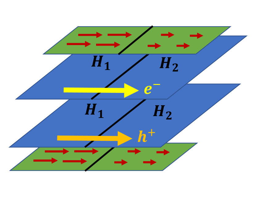
(a)

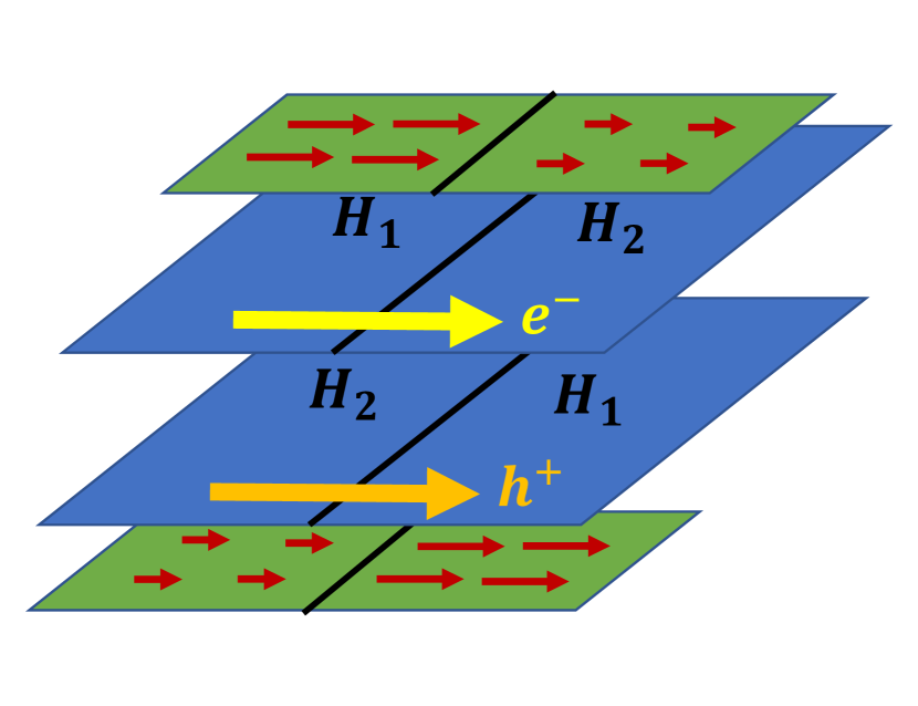
(b)

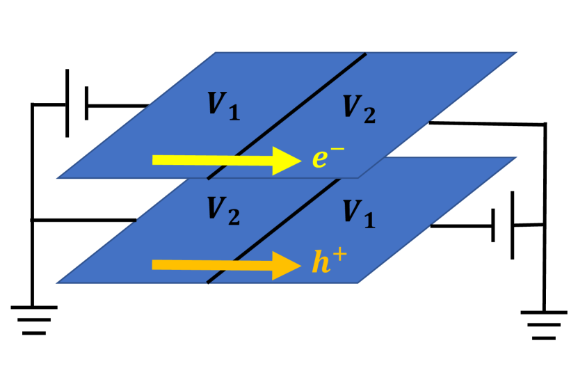
(c)

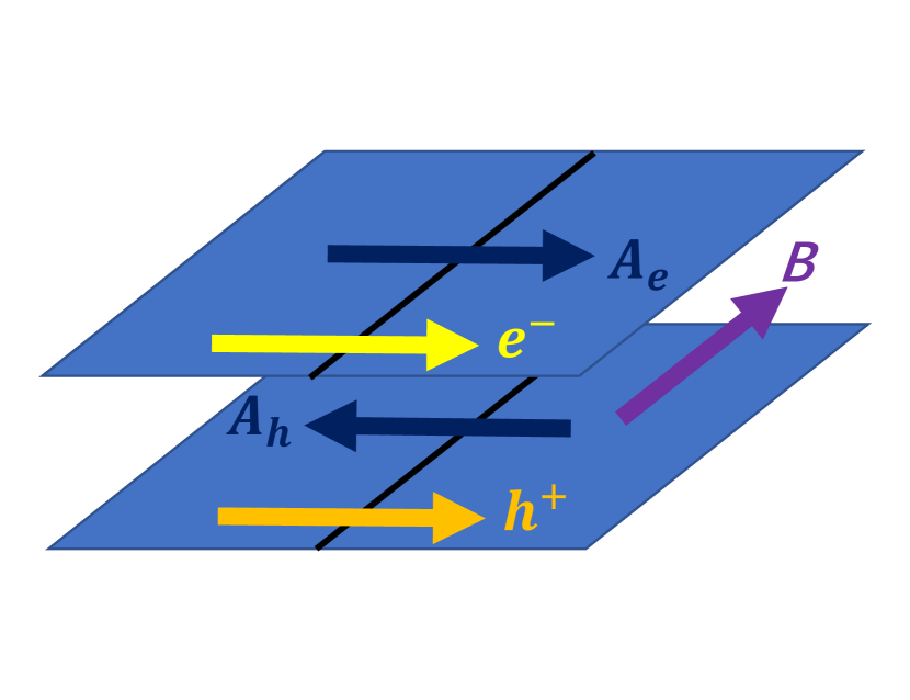
(d)

Figure 7: Four ways to induce the counterflow charge Josephson currents. (a) By a spin voltage across the junction, $V_{S}=V_{Sb}+V_{Sa}$ in the transverse phase. (b) By a spin voltage across the junction, $V_{S}=V_{Sb}-V_{Sa}$ in the longitudinal phase. (c) By a charge voltage across the junction, $V_{C}=V_{Cb}-V_{Ca}$. (d) By the transverse magnetic flux through the junction, $\Psi$.

.7 Solutions of the spin-charge coupled Josephson equations: $V_{S}$-$I_{C}$ conversion

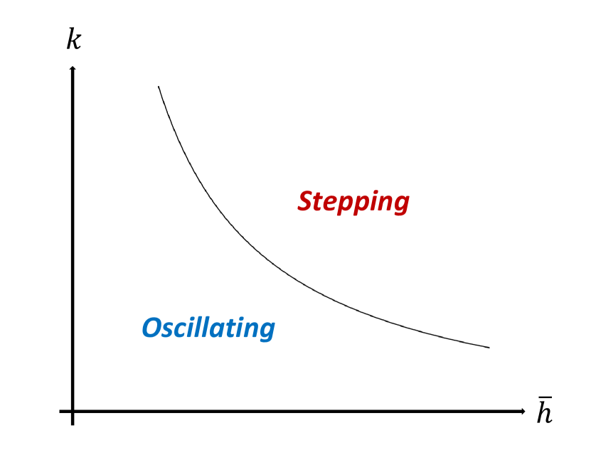
(a)

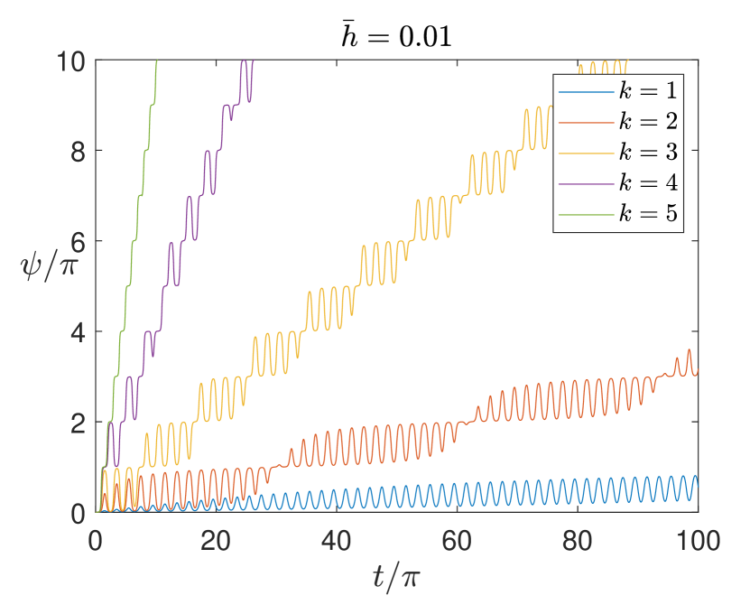
(b)

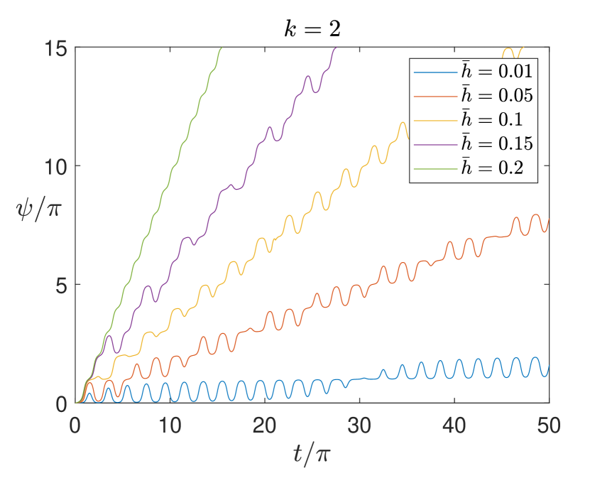
(c)

Figure 8: (a) Schematic crossover diagram of a solution of Eq. (.7.3) in favor for $\psi(t)$. In a ‘oscillating region’ ($k\bar{h}\ll 1$), $\psi(t)$ comprises of two oscillations with short periodicity $T_{1}=2\pi$ and a longer periodicity $T_{2}={\cal O}(\pi/(k\bar{h}))$. In a ‘stepping region’ ($k\bar{h}\geq 1$), $\psi(t)$ takes a constant value of $n\pi$ around $t=n\pi$ and $\psi(t)$ increases abruptly from $n\pi$ to $(n+1)\pi$ around $t=(2n+1)\pi/2$. (b, c) A crossover from the oscillating region to the stepping region.

In this section, we solve the spin-charge coupled Josephson equations under a particular physical circumstance depicted in Fig. 2(a) of the main text. Thereby, the electron layer is externally connected to a closed electric circuit with an electric resistance $R_{a}$, and the hole layer is connected to another external circuit with an electric resistance $R_{b}$. An exchange field is induced in the hole layer through a magnetic proximity effect. By using a spatial variation of the exchange field, we apply a spin voltage across the junction between two domains; $V_{Sb}\neq 0$, $V_{Sa}=0$. According to the Josephson equations, the spin voltage results in a linear increase of $\tilde{\varphi}_{0}$ in time, which leads to both a.c. charge supercurent $I_{C}$ and a.c. spin supercurrent $I_{S}$. Leads in the external circuits do not conserve spin angular momenta in general. Thus, the spin component of the supercurrents injected into the external circuits shall decay quickly and it has no significant impact on the spin voltage. In this respect, we can assume that the spin voltage is determined only by the static exchange field by the proximity effect. $V_{S}=V_{Sb}\pm V_{Sa}$ thus given is constant in time. On the one hand, the charge component of the supercurrents induce an a.c. charge voltages in both electron and hole layers; $V_{Ca}=I_{Ca}R_{a}$ and $V_{Cb}=I_{Cb}R_{b}$. From $V_{C}=V_{Cb}-V_{Ca}$ and $I_{Ca}=-I_{Cb}=-I_{C}$, Eqs. (.6.38, .6.40) lead to a closed equation of motion for $\tilde{\psi}(t)$,

$$\frac{d\tilde{\psi}}{dt}=-I_{0}R\!\ \bigg{(}\sin\big(\tilde{\psi}\big{missing})\cos\big(\mp V_{S}t\big{missing})-\bar{h}\!\ \cos\big(\tilde{\psi}\big{missing})\sin\big(\mp V_{S}t\big{missing})\bigg{)},$$ (.7.1)

with $R\equiv R_{a}+R_{b}$. With rescaling of the relevant variables,

$$V_{S}t\equiv s,\quad k\equiv\frac{I_{0}R}{V_{S}},$$ (.7.2)

we have

$$\frac{d\tilde{\psi}}{ds}=-k\!\ \bigg{(}\sin\big(\tilde{\psi}\big{missing})\cos\big(s\big{missing})\pm\bar{h}\!\ \cos\big(\tilde{\psi}\big{missing})\sin\big(s\big{missing})\bigg{)}.$$ (.7.3)

In this section, we will describe (numerical) solution of this non-linear differential equation in favor for $\tilde{\psi}(s)$. Without loss of generality, we take the minus sign, i.e. the longitudinal phase (Eq. (.3)) in Eq. (.7.3), and $k$ and $\bar{h}$ can be assumed to be positive. $\bar{h}\equiv{\sf{h}}(1+A_{x}/A_{0})$ is supposed to be much small than 1; $|{\sf{h}}|\equiv|h^{\prime}/h_{c}|\ll 1$ and $A_{x}/A_{0}={\cal O}(1)$. Thus, we discuss the solution only in a region of $0\leq\bar{h}\ll 1$. For simplicity, we remove the tilde from $\tilde{\psi}(s)$ and call $s$ as $t$, $\tilde{\psi}(s)\rightarrow\psi(t)$.

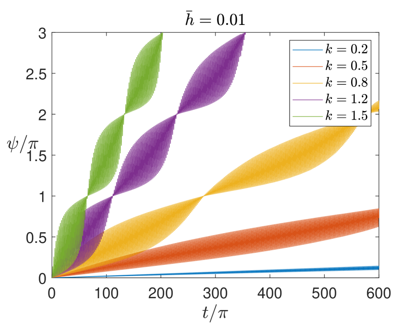
(a)

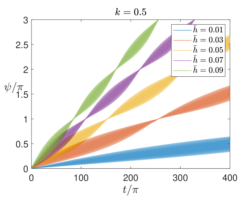
(b)

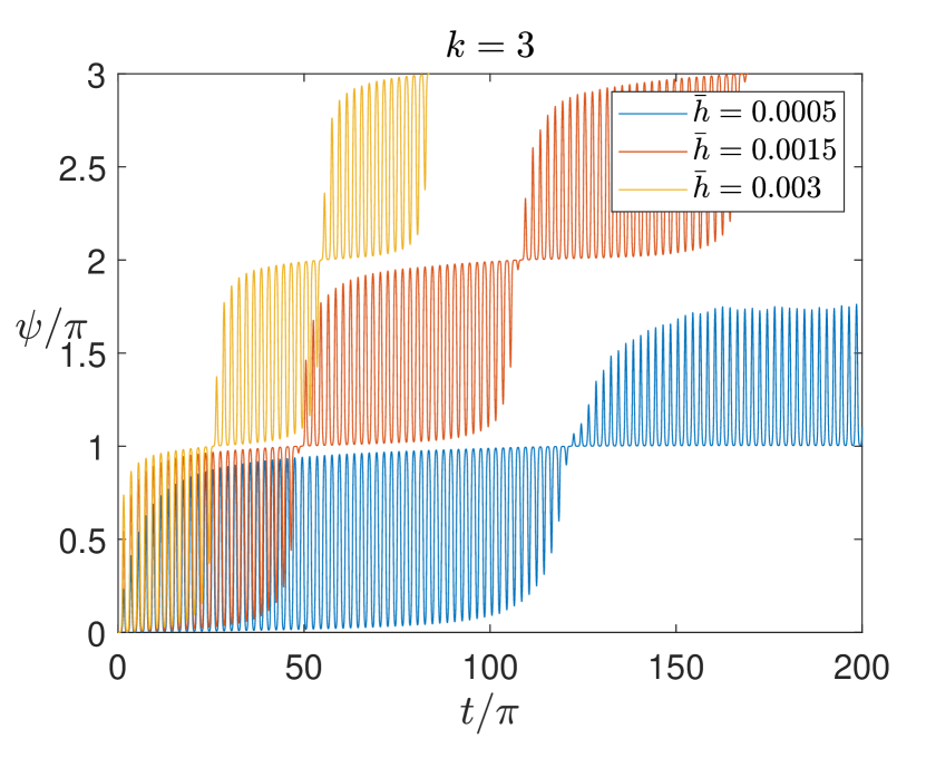
(c)

Figure 9: $\psi(t)$ in the oscillating region in a longer time scale. $\psi(t)$ comprises of two oscillations with a short periodicity and a longer periodicity. The short periodicity is $T_{1}=2\pi$ (see Fig. 10), while the longer periodicity changes with $k\bar{h}$.

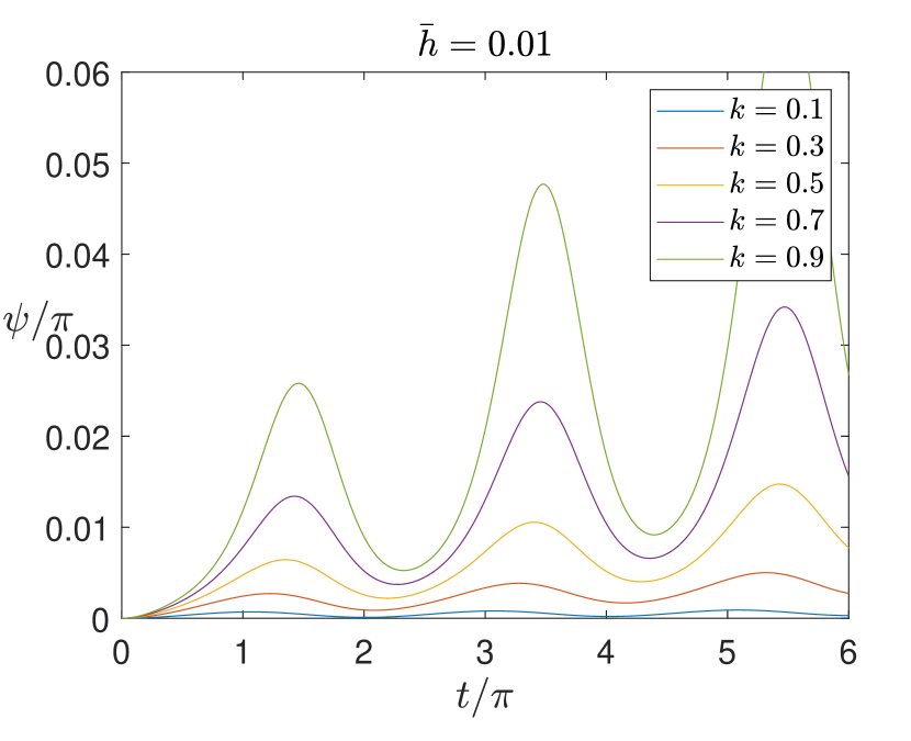
(a)

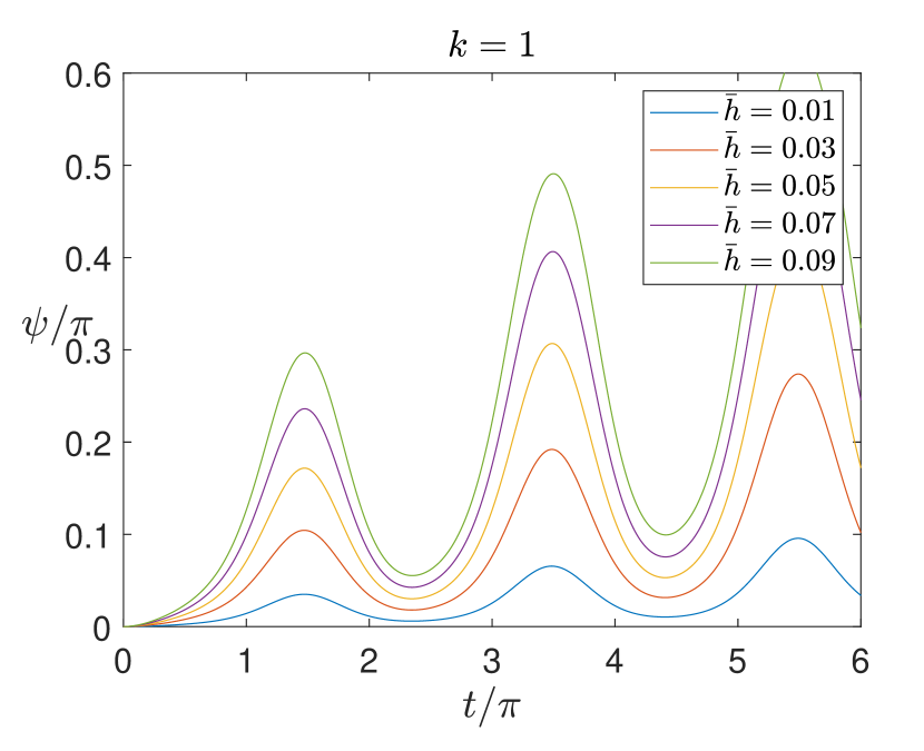
(b)

Figure 10: $\psi(t)$ in the oscillating region in a shorter time scale. The short periodicity $T_{1}$ is around $2\pi$.

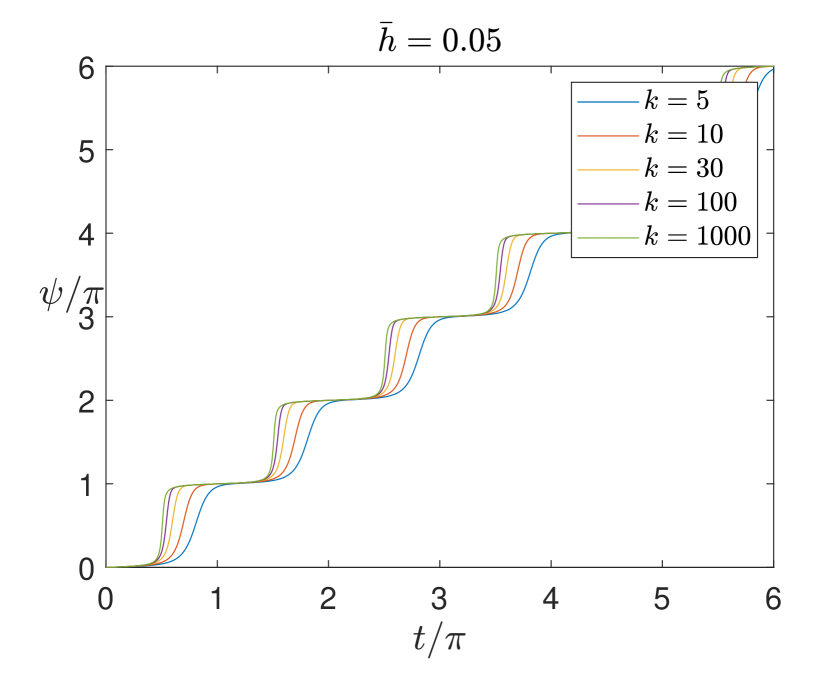
(a)

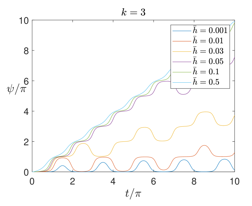
(b)

Figure 11: (a) $\psi(t)$ in the stepping region. $\psi(t)$ takes a constant value of $n\pi$ around $t=n\pi$, while it changes abruptly from $n\pi$ to $(n+1)\pi$ around $t=(2n+1)\pi/2$. (b) $\psi(t)$ in the stepping region ($\bar{h}=0.5,\!\ 0.1,\!\ 0.05$), in the crossover region $(\bar{h}=0.03)$ and in the oscillating region ($\bar{h}=0.01,\!\ 0.001$).

When $\bar{h}=0$, the solution is oscillatory in time with $2\pi$ periodicity ($T_{1}=2\pi$);

$$\frac{\psi(t)}{2}=\arctan(\tan(\frac{\psi(0)}{2})e^{-k\sin(t)}).$$ (.7.4)

The solution respects a time-reversal symmetry $\psi(\pi-t)=\psi(t)$. The amplitude of the oscillation gets larger for larger $k$, while it is always bounded by $\pi$; $\psi(t)$ is in the same branch of the arctan function of Eq. (.7.4). A finite $\bar{h}$ breaks the time-reversal symmetry, and the solution acquires a $t$-asymmetric component that increases linearly in time $t$. The form of the differential equation indicates that the $t$-asymmetric component must be scaled by $k\bar{h}t$ for $k\bar{h}\ll 1$; without loss of generality, we take $\psi(0)=0$, such that $\langle\psi(t)\rangle\sim k\bar{h}t$, where $\langle\psi(t)\rangle$ is an average of $\psi(t)$ over a time scale much longer than $T_{1}$ and much shorter than $1/(k\bar{h})$. $\langle\psi(t)\rangle$ modifies the short-periodicity ($T_{1}$) ocillating amplitute by the factor $\mathrm{sin}(\psi)$ in front of $\mathrm{cos}(t)$. Overall behaviours of numerical solutions are consistent with this indication (see Fig. 9). Due to the $t$-asymmetric component, the solution with finite $\bar{h}$ with $k\bar{h}\ll 1$ comprises of two oscillations: one with the shorter periodicity $T_{1}=2\pi$, and the other with a longer peridocity, $T_{2}={\cal O}(\pi/(k\bar{h}))$ (Figs. 9, 10).

When $k\bar{h}\ll 1$, the two oscillations are clearly distinguishable (‘oscillating region’). When $k\bar{h}={\cal O}(1)$, the two periodicities become on the same order and the solution shows a crossover from the oscillating region to a ‘stepping region’ (Figs. 8(b), 8(c)). When $k\gg k\bar{h}>1$, the solution converges into the stepping behavior, where $\psi(t)$ shows a plateau ($\psi(t)=n\pi$) around $t=n\pi$, and $\psi(t)$ increases abruptly from $n\pi$ to $(n+1)\pi$ around $t=(2n+1)\pi/2$ (Fig. 11).

.8 Derivation of classical ground-state phase diagram with Rashba coupling

In this section, we describe the minimization of the Lagrangian in the presence of the antisymmetric vector-product (AVP) type interaction ($D\neq 0$), Eq. (.2). In the absence of the AVP type interaction ($D=0$), the classical Lagrangian is minimized by spatial uniform configurations of $\vec{\Phi}^{\prime}(\vec{r})$ and $\vec{\Phi}^{\prime\prime}(\vec{r})$. To discuss the minimization in the presence of the AVP type interaction, let us decompose these four-component vectors into their amplitude parts ($\Phi^{\prime}(\vec{r})$ and $\Phi^{\prime\prime}(\vec{r})$) and four-component unit vector parts ($\vec{\psi}^{\prime}(\vec{r})$ and $\vec{\psi}^{\prime\prime}(\vec{r})$); $\vec{\Phi}^{\prime}(\vec{r})\equiv\Phi^{\prime}(\vec{r})\vec{\psi}^{\prime}(\vec{r})$ and $\vec{\Phi}^{\prime\prime}(\vec{r})\equiv\Phi^{\prime\prime}(\vec{r})\vec{\psi}^{\prime\prime}(\vec{r})$. Spatial gradients of the amplitude parts do not lower the AVP type interaction energy because of its anti-symmetric form, e.g.

$$D[(\Phi^{\prime}\psi^{\prime}_{z})\partial_{x}(\Phi^{\prime}\psi^{\prime}_{x})-(\Phi^{\prime}\psi^{\prime}_{x})\partial_{x}(\Phi^{\prime}\psi^{\prime}_{z})]=D(\Phi^{\prime})^{2}[\psi^{\prime}_{z}\partial_{x}(\psi^{\prime}_{x})-\psi^{\prime}_{x}\partial_{x}(\psi^{\prime}_{z})].$$ (.8.1)

Thus, we take the amplitude parts to be spatially uniform, $\vec{\Phi}^{\prime}(\vec{r})\equiv\Phi^{\prime}\vec{\psi}^{\prime}(\vec{r})$ and $\vec{\Phi}^{\prime\prime}(\vec{r})\equiv\Phi^{\prime\prime}\vec{\psi}^{\prime\prime}(\vec{r})$.

The classical Lagrangian of Eq. (.2) consists of three parts:

$$\frac{S}{\beta}=S_{0}[\vec{\Phi}^{\prime},\vec{\Phi}^{\prime}]+S_{1}[\vec{\Phi}^{\prime}]+S_{1}[\vec{\Phi}^{\prime\prime}]\equiv\int\mathrm{d}^{2}\vec{r}[\mathcal{L}_{0}(\vec{\Phi}^{\prime},\vec{\Phi}^{\prime\prime})+\mathcal{L}_{1}(\vec{\Phi}^{\prime},\partial_{i}\vec{\Phi}^{\prime})+\mathcal{L}_{1}(\vec{\Phi}^{\prime\prime},\partial_{i}\vec{\Phi}^{\prime\prime})].\quad(i=x,y)$$ (.8.2)

The first part describes a coupling between $\vec{\Phi}^{\prime}(\vec{r})$ and $\vec{\Phi}^{\prime\prime}(\vec{r})$. It is free from the spatial gradients of the fields,

$$S_{0}[\vec{\Phi}^{\prime},\vec{\Phi}^{\prime}] \equiv\int\mathrm{d}^{2}\vec{r}\mathcal{L}_{0}(\vec{\Phi}^{\prime},\vec{\Phi}^{\prime\prime}),$$

$${\cal L}_{0}(\vec{\Phi}^{\prime},\vec{\Phi}^{\prime\prime}) =A({\Phi^{\prime}}^{2}+{\Phi^{\prime\prime}}^{2})+B[{\Phi^{\prime}}^{4}+{\Phi^{\prime\prime}}^{4}+6{\Phi^{\prime}}^{2}{\Phi^{\prime\prime}}^{2}]-2\Phi^{\prime}\Phi^{\prime\prime}g(\Phi^{\prime},\Phi^{\prime\prime},\vec{\psi}^{\prime},\vec{\psi}^{\prime\prime}),$$

$$g(\Phi^{\prime},\Phi^{\prime\prime},\vec{\psi}^{\prime},\vec{\psi}^{\prime\prime}) =2B\Phi^{\prime}\Phi^{\prime\prime}\big{(}\vec{\psi}^{\prime}({\vec{r}})\cdot\vec{\psi}^{\prime\prime}(\vec{r})\big{)}^{2}+h\big{(}\psi^{\prime}_{y}(\vec{r})\psi^{\prime\prime}_{z}(\vec{r})-\psi^{\prime}_{z}(\vec{r})\psi^{\prime\prime}_{y}(\vec{r})\big{)}-h^{\prime}\big{(}\psi^{\prime}_{0}(\vec{r})\psi^{\prime\prime}_{x}(\vec{r})-\psi^{\prime}_{x}(\vec{r})\psi^{\prime\prime}_{0}(\vec{r})\big{)}.$$ (.8.3)

The other two parts depend on $\vec{\Phi}^{\prime}(\vec{r})$ and $\vec{\Phi}^{\prime\prime}(\vec{r})$ separately and they depend on their spatial gradients, e.g.

$$S_{1}[\Phi^{\prime}\vec{\psi}^{\prime}]=\Phi^{\prime 2}\int\mathrm{d}^{2}\vec{r}\{\lambda(\nabla\psi^{\prime}_{\mu})\cdot(\nabla\psi^{\prime}_{\mu})-D(\psi^{\prime}_{z}\partial_{x}\psi^{\prime}_{x}-\psi^{\prime}_{x}\partial_{x}\psi^{\prime}_{z}-\psi^{\prime}_{y}\partial_{y}\psi^{\prime}_{z}+\psi^{\prime}_{z}\partial_{y}\psi^{\prime}_{y}+\psi^{\prime}_{x}\partial_{y}\psi^{\prime}_{0}-\psi^{\prime}_{y}\partial_{x}\psi^{\prime}_{0}+\psi^{\prime}_{0}\partial_{x}\psi^{\prime}_{y}-\psi^{\prime}_{0}\partial_{y}\psi^{\prime}_{x})\}.$$ (.8.4)

We first minimize $S_{1}[\Phi^{\prime}\vec{\psi}^{\prime}]$ and $S_{1}[\Phi^{\prime\prime}\vec{\psi}^{\prime\prime}]$ in terms of the four-component vectors $\vec{\psi}^{\prime}$ and $\vec{\psi}^{\prime\prime}$ respectively. We then show that $\vec{\Phi}^{\prime}$ and $\vec{\Phi}^{\prime\prime}$ thus determined also maximally minimize $S_{0}[\vec{\Phi}^{\prime},\vec{\Phi}^{\prime}]$ by optimizing the amplitude parts, $\Phi^{\prime}$ and $\Phi^{\prime\prime}$.

To minimize $S_{1}[\Phi^{\prime}\vec{\psi}^{\prime}]$ in terms of $\vec{\psi}^{\prime}(\vec{r})\equiv(\psi^{\prime}_{0}(\vec{r}),\psi^{\prime}_{x}(\vec{r}),\psi^{\prime}_{y}(\vec{r}),\psi^{\prime}_{z}(\vec{r}))$, take the Fourier transformation of $\psi^{\prime}_{\mu}(\vec{r})$,

$$\psi^{\prime}_{\mu,\vec{k}}=\int\mathrm{d}^{2}\vec{r}\mathrm{e}^{-\mathrm{i}\vec{k}\cdot\vec{r}}\psi^{\prime}_{\mu}(\vec{r}),\quad\psi^{\prime}_{\mu}(\vec{r})=\frac{1}{V}\sum_{\vec{k}}\mathrm{e}^{\mathrm{i}\vec{k}\cdot\vec{r}}\psi^{\prime}_{\mu,\vec{k}},$$ (.8.5)

for $\mu=0,x,y,z$ with ${\psi^{\prime}}^{*}_{\mu,\vec{k}}=\psi^{\prime}_{\mu,-\vec{k}}$. The Fourier component $\psi^{\prime}_{\mu,\vec{k}}$ is given by two real-valued functions $\alpha_{\mu,\vec{k}}$ and $\beta_{\mu,\vec{k}}$ as $\psi^{\prime}_{\mu,\vec{k}}\equiv\alpha_{\mu,\vec{k}}+{\rm i}\beta_{\mu,\vec{k}}$. They are even and odd functions in $\vec{k}$ respectively. $S_{1}[\Phi^{\prime}\vec{\psi}^{\prime}]$ is given by these two functions:

$$S_{1}[\Phi^{\prime}\vec{\psi}^{\prime}] =\frac{2\Phi^{\prime 2}\lambda}{V}\sum_{k_{x}>0}k^{2}w^{2}_{\vec{k}}+\frac{4\Phi^{\prime 2}D}{V}\sum_{k_{x}>0}f(\alpha_{\mu,\vec{k}},\beta_{\mu,\vec{k}}),$$ (.8.6)

$$f(\alpha_{\mu,\vec{k}},\beta_{\mu,\vec{k}}) \equiv k_{x}(\alpha_{z,\vec{k}}\beta_{x,\vec{k}}-\alpha_{x,\vec{k}}\beta_{z,\vec{k}}+\alpha_{0,\vec{k}}\beta_{y,\vec{k}}-\alpha_{y,\vec{k}}\beta_{0,\vec{k}})+k_{y}(\alpha_{z,\vec{k}}\beta_{y,\vec{k}}-\alpha_{y,\vec{k}}\beta_{z,\vec{k}}+\alpha_{x,\vec{k}}\beta_{0,\vec{k}}-\alpha_{0,\vec{k}}\beta_{x,\vec{k}}),$$ (.8.7)

with $w^{2}_{\vec{k}}\equiv\sum_{\mu}(\alpha_{\mu,\vec{k}}\alpha_{\mu,\vec{k}}+\beta_{\mu,\vec{k}}\beta_{\mu,\vec{k}})$. For given $w_{\vec{k}}$, $f(\alpha_{\mu,\vec{k}},\beta_{\mu,\vec{k}})$ in Eq. (.8.6) shall be minimized for each $\hat{k}$ (the subscribe $\vec{k}$ will be omitted for convenience):

$$f(\alpha_{\mu},\beta_{\mu})=k_{x}(\alpha_{z}\beta_{x}-\alpha_{x}\beta_{z}+\alpha_{0}\beta_{y}-\alpha_{y}\beta_{0})+k_{y}(\alpha_{z}\beta_{y}-\alpha_{y}\beta_{z}-\alpha_{0}\beta_{x}+\alpha_{x}\beta_{0})=-\hat{k}\cdot(\hat{\alpha}^{\prime}\times\hat{\beta}^{\prime}+\alpha^{\prime}_{0}\hat{\beta}^{\prime}-\beta^{\prime}_{0}\hat{\alpha}^{\prime}).$$ (.8.8)

In the right hand side of Eq. (.8.8), the three-component vectors $\hat{\alpha}^{\prime}$, $\hat{\beta}^{\prime}$, $\hat{k}$ are introduced as,

$$\hat{\alpha}^{\prime}\equiv(\alpha^{\prime}_{x},\alpha^{\prime}_{y},\alpha^{\prime}_{z}),\quad\hat{\beta}^{\prime}\equiv(\beta^{\prime}_{x},\beta^{\prime}_{y},\beta^{\prime}_{z}),\quad\hat{k}\equiv(k_{x},k_{y},0)\equiv(\vec{k},0),$$

$$\alpha_{x}=\alpha^{\prime}_{y},\quad\alpha_{y}=-\alpha^{\prime}_{x},\quad\alpha_{z}=\alpha^{\prime}_{z},\quad\alpha_{0}=\alpha^{\prime}_{0};$$

$$\beta_{x}=\beta^{\prime}_{y},\quad\beta_{y}=-\beta^{\prime}_{x},\quad\beta_{z}=\beta^{\prime}_{z},\quad\beta_{0}=\beta^{\prime}_{0}.$$ (.8.9)

The function $f(\alpha_{\mu},\beta_{\mu})$ can be easily minimized for the special $\hat{k}$. For $\vec{k}=k\vec{e}_{x}$, it is minimized by

$$\alpha^{\prime}_{y}=\frac{w}{\sqrt{2}}\mathrm{cos}\zeta\mathrm{cos}\delta_{1},\quad\beta^{\prime}_{y}=-\frac{w}{\sqrt{2}}\mathrm{cos}\zeta\mathrm{sin}\delta_{1}, \quad\alpha^{\prime}_{z}=\frac{w}{\sqrt{2}}\mathrm{cos}\zeta\mathrm{sin}\delta_{1},\quad\beta^{\prime}_{z}=\frac{w}{\sqrt{2}}\mathrm{cos}\zeta\mathrm{cos}\delta_{1},$$

$$\alpha^{\prime}_{0}=\frac{w}{\sqrt{2}}\mathrm{sin}\zeta\mathrm{cos}\delta_{2},\quad\beta^{\prime}_{0}=-\frac{w}{\sqrt{2}}\mathrm{sin}\zeta\mathrm{sin}\delta_{2}, \quad\alpha^{\prime}_{x}=\frac{w}{\sqrt{2}}\mathrm{sin}\zeta\mathrm{sin}\delta_{2},\quad\beta^{\prime}_{x}=\frac{w}{\sqrt{2}}\mathrm{sin}\zeta\mathrm{cos}\delta_{2},$$ (.8.10)

with arbitrary U(1) variables $\zeta$, $\delta_{1}$ and $\delta_{2}$. For $\vec{k}=k\vec{e}_{y}$, we take a substitution of $\alpha^{\prime}_{1}\rightarrow\alpha^{\prime}_{2}$, $\alpha^{\prime}_{2}\rightarrow-\alpha^{\prime}_{1}$, $\alpha^{\prime}_{3}\rightarrow\alpha^{\prime}_{3}$, $\alpha^{\prime}_{0}\rightarrow\alpha^{\prime}_{0}$ in Eq. (.8), and change $\vec{\beta^{\prime}}$ similarly. For general $\vec{k}=k(\mathrm{cos}\omega\vec{e}_{x}+\mathrm{sin}\omega\vec{e}_{y})$, the function $f(\alpha_{\mu},\beta_{\mu})$ is minimized by a combination of these two,

$$\vec{\alpha}^{\prime}=\frac{w}{\sqrt{2}}[(-\mathrm{sin}\omega\mathrm{cos}\zeta\mathrm{cos}\delta_{1}+\mathrm{cos}\omega\mathrm{sin}\zeta\mathrm{sin}\delta_{2})\vec{e}_{x}+(\mathrm{sin}\omega\mathrm{sin}\zeta\mathrm{sin}\delta_{2}+\mathrm{cos}\omega\mathrm{cos}\zeta\mathrm{cos}\delta_{1})\vec{e}_{y}+\mathrm{cos}\zeta\mathrm{sin}\delta_{1}\vec{e}_{z}+\mathrm{sin}\zeta\mathrm{cos}\delta_{2}\vec{e}_{0}],$$ (.8.11)

$$\vec{\beta}^{\prime}=\frac{w}{\sqrt{2}}[(\mathrm{sin}\omega\mathrm{cos}\zeta\mathrm{sin}\delta_{1}+\mathrm{cos}\omega\mathrm{sin}\zeta\mathrm{cos}\delta_{2})\vec{e}_{x}+(\mathrm{sin}\omega\mathrm{sin}\zeta\mathrm{cos}\delta_{2}-\mathrm{cos}\omega\mathrm{cos}\zeta\mathrm{sin}\delta_{1})\vec{e}_{y}+\mathrm{cos}\zeta\mathrm{cos}\delta_{1}\vec{e}_{z}-\mathrm{sin}\zeta\mathrm{sin}\delta_{2}\vec{e}_{0}].$$ (.8.12)

With the solution Eqs. (.8.11–.8.12), $S_{1}[\Phi^{\prime}\vec{\psi}^{\prime}(\vec{r})]$ is minimized by the following $\vec{\psi}^{\prime}(\vec{r})$ for a given $\Phi^{\prime}$ and $w_{\vec{k}}$:

$$\vec{\psi}^{\prime}(\vec{r}) =\frac{1}{V}\sum_{k_{x}>0}\sqrt{2}w_{\vec{k}}\{[-\mathrm{sin}\omega\mathrm{sin}\zeta\mathrm{sin}(\vec{k}\cdot\vec{r}-\delta_{2})+\mathrm{cos}\omega\mathrm{cos}\zeta\mathrm{cos}(\vec{k}\cdot\vec{r}-\delta_{1})]\vec{e}_{x}$$

$$+[\mathrm{sin}\omega\mathrm{cos}\zeta\mathrm{cos}(\vec{k}\cdot\vec{r}-\delta_{1})+\mathrm{cos}\omega\mathrm{sin}\zeta\mathrm{sin}(\vec{k}\cdot\vec{r}-\delta_{2})]\vec{e}_{y}-\mathrm{cos}\zeta\mathrm{sin}(\vec{k}\cdot\vec{r}-\delta_{1})\vec{e}_{z}+\mathrm{sin}\zeta\mathrm{cos}(\vec{k}\cdot\vec{r}-\delta_{2})\vec{e}_{0}\},$$ (.8.13)

$$S_{1}[\Phi^{\prime}\vec{\psi}^{\prime}(\vec{r})]=\frac{2\Phi^{\prime 2}}{V}\sum_{k_{x}>0}\big{(}\lambda k^{2}-Dk\big{)}\!\ w_{\vec{k}}^{2}.$$ (.8.14)

Here $\omega$ in Eq. (.8) is a function of $\vec{k}/k$; $\vec{k}\equiv k(\mathrm{cos}\omega\vec{e}_{x}+\mathrm{sin}\omega\vec{e}_{y})$, while $\zeta$, $\delta_{1}$ and $\delta_{2}$ are arbitrary functions of $\vec{k}$. From Eq. (.8.14), $S_{1}[\Phi^{\prime}\vec{\psi}^{\prime}(\vec{r})]$ can be maximally minimized by those $w_{\vec{k}}$ that is non-zero only when $k=D/(2\lambda)$;

$$\vec{k}=k(\mathrm{cos}\omega\vec{e}_{x}+\mathrm{sin}\omega\vec{e}_{y})=\frac{D}{2\lambda}(\mathrm{cos}\omega\vec{e}_{x}+\mathrm{sin}\omega\vec{e}_{y}).$$ (.8.15)

The action thus minimized depends only on $\Phi^{\prime}$,

$$S_{1}[\Phi^{\prime}\vec{\psi}^{\prime}(\vec{r})]=-\frac{\Phi^{\prime 2}D^{2}}{2\lambda V}\sum_{k_{x}>0}w_{\vec{k}}^{2}=-\frac{\Phi^{\prime 2}D^{2}V}{4\lambda}.$$ (.8.16)

In the right hand side, we use a global constraint, $\sum_{\vec{k}}w^{2}_{\vec{k}}=V^{2}$, that comes from the local constraint $\sum_{\mu}\psi^{\prime}_{\mu}(\vec{r})\psi^{\prime}_{\mu}(\vec{r})=1$,

$$\sum_{\mu}\int\mathrm{d}^{2}\vec{r}\psi^{\prime}_{\mu}(\vec{r})\psi^{\prime}_{\mu}(\vec{r})=\frac{1}{V}\sum_{\mu,\vec{k}}{\psi^{\prime}}^{*}_{\mu,\vec{k}}\psi^{\prime}_{\mu,\vec{k}}=\frac{1}{V}\sum_{\vec{k}}w^{2}_{\vec{k}}=V.$$ (.8.17)

In Sec. .11, we show that it is impossible that $\psi_{\mu}(\vec{r})$ given by Eq. (.8) consists of two wavevector Fourier components. Specifically, we prove that if $\vec{\psi}(\vec{r})$ in Eq. (.8) consists of the two wavevector Fourier components, $\vec{k}_{1}$ and $\vec{k}_{2}$;

$$w_{\vec{k}}=\left\{\begin{array}[]{cl}0&{\rm for}\!\ \!\ \vec{k}\neq\vec{k}_{1}\!\ \!\ {\rm and}\!\ \!\ \vec{k}\neq\vec{k}_{2},\\ w_{1}\neq 0&{\rm for}\!\ \!\ \vec{k}=\vec{k}_{1},\\ w_{2}\neq 0&{\rm for}\!\ \!\ \vec{k}=\vec{k}_{2}\neq\vec{k}_{1},-\vec{k}_{1},\\ \end{array}\right.$$ (.8.21)

$\vec{\psi}(\vec{r})$ thus given cannot satisfy the local constraint $(\vec{\psi}(\vec{r})\cdot\vec{\psi}(\vec{r})=1)$ in any way. The conclusion can be generalized into a case with more than the two momenta. Thus, we regard $\vec{\psi}(\vec{r})$ is composed only of one component of momentum $\vec{k}$ on $|\vec{k}|=D/(2\lambda)$ and take $w=\frac{V}{\sqrt{2}}$ from the global constraint. In conclusion, $S_{1}[\Phi^{\prime}\vec{\psi}^{\prime}(\vec{r})]$ is maximally minimized by,

$$\vec{\psi}^{\prime}(\vec{r}) =\{[-\mathrm{sin}\omega^{\prime}\mathrm{sin}\zeta\mathrm{sin}(\vec{k}^{\prime}\cdot\vec{r}-\delta^{\prime}_{2})+\mathrm{cos}\omega^{\prime}\mathrm{cos}\zeta^{\prime}\mathrm{cos}(\vec{k}^{\prime}\cdot\vec{r}-\delta^{\prime}_{1})]\vec{e}_{x}$$

$$+[\mathrm{sin}\omega^{\prime}\mathrm{cos}\zeta^{\prime}\mathrm{cos}(\vec{k}^{\prime}\cdot\vec{r}-\delta^{\prime}_{1})+\mathrm{cos}\omega^{\prime}\mathrm{sin}\zeta^{\prime}\mathrm{sin}(\vec{k}^{\prime}\cdot\vec{r}-\delta^{\prime}_{2})]\vec{e}_{y}-\mathrm{cos}\zeta^{\prime}\mathrm{sin}(\vec{k}^{\prime}\cdot\vec{r}-\delta^{\prime}_{1})\vec{e}_{z}+\mathrm{sin}\zeta^{\prime}\mathrm{cos}(\vec{k}^{\prime}\cdot\vec{r}-\delta^{\prime}_{2})\vec{e}_{0}\},$$ (.8.22)

with $\vec{k}^{\prime}=\frac{D}{2\lambda}(\cos\omega^{\prime}\vec{e}_{x}+\sin\omega^{\prime}\vec{e}_{y})$ together with arbitrary U(1) phase variables, $\zeta^{\prime}$, $\delta^{\prime}_{1}$ and $\delta^{\prime}_{2}$. Note that this satisfies the local constraint, $\vec{\psi}(\vec{r})\cdot\vec{\psi}(\vec{r})=1$. Likewise, $S_{1}[\Phi^{\prime\prime}\vec{\psi}^{\prime\prime}(\vec{r})]$ is maximally minimized by $\psi^{\prime\prime}(\vec{r})$ given by the same type of the unit vector as Eq. (.8) with another set of the U(1) variables of $\omega^{\prime\prime}$ ($\vec{k}^{\prime\prime}$), $\zeta^{\prime\prime}$, $\delta^{\prime\prime}_{1}$ and $\delta^{\prime\prime}_{2}$.

Finally, we minimize $S_{0}[\vec{\Phi}^{\prime},\vec{\Phi^{\prime\prime}}]$ within a ‘manifold’ of Eq. (.8) for $\vec{\Phi}^{\prime}(\vec{r})\equiv\Phi^{\prime}\vec{\psi}^{\prime}(\vec{r})$ and that for $\vec{\Phi}^{\prime\prime}(\vec{r})\equiv\Phi^{\prime\prime}\vec{\psi}^{\prime\prime}(\vec{r})$. The minimization is carried out in a parameter space subtended by $\omega^{\prime}$ ($\vec{k}^{\prime}$), $\zeta^{\prime}$, $\delta^{\prime}_{1}$, $\delta^{\prime}_{2}$, $\omega^{\prime\prime}$ ($\vec{k}^{\prime\prime}$), $\zeta^{\prime\prime}$, $\delta^{\prime\prime}_{1}$, $\delta^{\prime\prime}_{2}$, $\Phi^{\prime}$ and $\Phi^{\prime\prime}$. To begin with, we consider to maximize $g$ in Eq. (.8.3) at a given spatial point $\vec{r}$. The maximization leads to $\omega^{\prime}=\omega^{\prime\prime}=\pi/2$ ($\vec{k}^{\prime}=\vec{k}^{\prime\prime}=\frac{D}{2\lambda}\vec{e}_{y}$), while $\zeta^{\prime}=\zeta^{\prime\prime}=\pi/2$ for $|h|\leq|h^{\prime}|$, and $\zeta^{\prime}=\zeta^{\prime\prime}=0$ for $|h^{\prime}|\leq|h|$. For each of these two cases, we then maximize $g$ in Eq. (.8.3) in terms of $\delta^{\prime}_{2}-\delta^{\prime\prime}_{2}$ and $\delta^{\prime}_{1}-\delta^{\prime\prime}_{1}$ respectively, and finally minimize the whole action in terms of $\Phi^{\prime}$ and $\Phi^{\prime\prime}$;

$$s \equiv\frac{S}{V}=A^{\prime}(\Phi^{\prime 2}+\Phi^{\prime\prime 2})+B(\Phi^{\prime 4}+\Phi^{\prime\prime 4}+6\Phi^{\prime 2}\Phi^{\prime\prime 2})-2\Phi^{\prime}\Phi^{\prime\prime}g,$$

$$g \equiv\left\{\begin{array}[]{cc}2B\Phi^{\prime}\Phi^{\prime\prime}\cos(\delta^{\prime}_{1}-\delta^{\prime\prime}_{1})+h\sin(\delta^{\prime}_{1}-\delta^{\prime\prime}_{1})&{\rm when}\!\ \!\ \!\ |h^{\prime}|<|h|,\\ 2B\Phi^{\prime}\Phi^{\prime\prime}\cos(\delta^{\prime}_{2}-\delta^{\prime\prime}_{2})-h^{\prime}\sin(\delta^{\prime}_{2}-\delta^{\prime\prime}_{2})&{\rm when}\!\ \!\ \!\ |h|<|h^{\prime}|,\\ \end{array}\right.$$ (.8.25)

with $A^{\prime}=-(\alpha-\frac{2}{g}+\frac{D^{2}}{4\lambda})$. Here the $D^{2}$ term in $A^{\prime}$ comes from Eq. (.8.16). The maximization of $g$ in terms of $\delta^{\prime}_{2}-\delta^{\prime\prime}_{2}=\alpha_{1}$ and $\delta^{\prime}_{1}-\delta^{\prime\prime}_{1}=\alpha_{2}$ and the minimization of the classical action $s$ in terms of $\Phi^{\prime}$ and $\Phi^{\prime\prime}$ are essentially same as in Eqs. (.3.8–.3.19). Thereby, Eqs. (.3–.3.23) are still valid classical solutions, except for the following substitutions,

$$\varphi_{0}\rightarrow\varphi_{0}-Ky,\quad K\equiv\frac{D}{2\lambda},$$ (.8.26)

$$h_{c}=\alpha-\frac{2}{g}\rightarrow h_{c}=\alpha-\frac{2}{g}+\frac{D^{2}}{4\lambda}.$$ (.8.27)

To summarize, we have the following four phases.
For $|h^{\prime}|<|h|<h_{c}$ (regular helicoidal phase):

$$\vec{\phi}=\rho\mathrm{cos}\theta(\mathrm{cos}(\varphi_{0}-Ky)\vec{e}_{y}+\mathrm{sin}(\varphi_{0}-Ky)\vec{e}_{z})+\mathrm{i}\rho\mathrm{sin}\theta[\mathrm{cos}(\varphi+\varphi_{0}-Ky)\vec{e}_{y}+\mathrm{sin}(\varphi+\varphi_{0}-Ky)\vec{e}_{z}],$$

$$\rho=\sqrt{\frac{h_{c}}{2|\gamma|}},\quad\mathrm{sin}\varphi\mathrm{sin}2\theta=\frac{h}{h_{c}}.$$ (.8.28)

For $|h|<|h^{\prime}|<h_{c}$ (regular helical phase):

$$\vec{\phi}=\rho[-\mathrm{sin}\theta\mathrm{cos}(\varphi+\varphi_{0}-Ky)\vec{e}_{0}+\mathrm{cos}\theta\mathrm{sin}(\varphi_{0}-Ky)\vec{e}_{x}]+\mathrm{i}\rho[\mathrm{cos}\theta\mathrm{cos}(\varphi_{0}-Ky)\vec{e}_{0}+\mathrm{sin}\theta\mathrm{sin}(\varphi+\varphi_{0}-Ky)\vec{e}_{x}],$$

$$\rho=\sqrt{\frac{h_{c}}{2|\gamma|}},\quad\mathrm{sin}\varphi\mathrm{sin}2\theta=-\frac{h^{\prime}}{h_{c}}.$$ (.8.29)

For $|h^{\prime}|<|h|$, $h_{c}<|h|$ (saturated helicoidal phase):

$$\vec{\phi}=\rho(\mathrm{cos}(\varphi_{0}-Ky)\vec{e}_{y}+\mathrm{sin}(\varphi_{0}-Ky)\vec{e}_{z})-\mathrm{i}\rho\mathrm{sgn}(h)[\mathrm{sin}(\varphi_{0}-Ky)\vec{e}_{y}-\mathrm{cos}(\varphi_{0}-Ky)\vec{e}_{z}],\quad\rho=\sqrt{\frac{h_{c}+|h|}{8|\gamma|}}.$$ (.8.30)

For $|h|<|h^{\prime}|$, $h_{c}<|h^{\prime}|$ (saturated helical phase):

$$\vec{\phi}=\rho[\mathrm{sgn}(-h^{\prime})\mathrm{sin}(\varphi_{0}-Ky)\vec{e}_{0}+\mathrm{sin}(\varphi_{0}-Ky)\vec{e}_{x}]+\mathrm{i}\rho[\mathrm{cos}(\varphi_{0}-Ky)\vec{e}_{0}+\mathrm{sgn}(-h^{\prime})\mathrm{cos}(\varphi_{0}-Ky)\vec{e}_{x}],\quad\rho=\sqrt{\frac{h_{c}+|h^{\prime}|}{8|\gamma|}}.$$ (.8.31)

Here we call ground-state configurations of Eqs. (.8, .8.30) with the substitutions as regular and saturated helicoidal phase and those of Eqs. (.8, .8.31) as regular and saturated helical phase. Both helical and helicoidal phases have a nonzero momentum $K$, breaking the translational symmetry along $y$-axis. The phase diagram with $D\neq 0$ is given by Fig. 5(a) where ‘transverse’ and ‘longitudinal’ are replaced by ‘helicoidal’ and ‘helical’ respectively. The helicoidal phases were introduced and studied in Ref. [77]. A schematic picture of the helical phase is shown in Fig. 5(b).

.9 Derivation of spin-charge coupled Josephson equation with Rashba coupling

In this section, we derive spin-charge coupled Josephson equations in the helicoidal and helical phases. We first apply Noether’s theorem to the $\phi^{4}$-type effective Lagrangian, Eq. (.2), to express (conserved) charge and spin currents in terms of the four-components excitonic fields and their spatial gradient terms. We then substitute the classical solutions, Eqs. (.8–.8.31), into the expressions. This leads to the spin-charge coupled Josephson equations in the helical and helicoidal phases.

In practice, the magnetic exchange fields within the $xy$ plane can be experimentally controlled by an external magnetic field in the plane. The magnetic field causes magnetic vector potentials in the electron and hole layers. In the presence of the vector potentials, $\partial_{i}$ in Eqs. (1, .1.1) ($i=x,y$) are replaced by $\partial_{i}+{\mathrm{i}}A_{a,i}$ in the electron layer and by $\partial_{i}+{\mathrm{i}}A_{b,i}$ in the hole layer. The two vector potentials, $A_{a,i}$ and $A_{b,i}$, are generally different from each other, as the electron and hole layers are spatially separated along the $z$ direction. An integral of the difference between them, $\tilde{A}_{i}\equiv A_{b,i}-A_{a,i}$, is the magnetic flux penetrating through the separation layer. The difference appears in the $\phi^{4}$-type effective Lagrangian in a covariant way; $\partial_{i}$ in Eq. (.2) is replaced by $\partial_{i}-{\mathrm{i}}\tilde{A}_{i}$.

Noether’s theorem associates a global continuous symmetry in Lagrangian ${\cal L}(\vec{\phi},\partial_{i}\vec{\phi})$ with a conserved current. [83] Suppose that a Lagrangian is invariant under the following transformation,

$$\phi_{\nu}\rightarrow\phi_{\nu}+\epsilon\Delta\phi_{\nu},\quad\phi_{\nu}^{*}\rightarrow\phi_{\nu}^{*}+\epsilon\Delta\phi_{\nu}^{*},$$ (.9.1)

with a small $\epsilon$. Noether’s theorem dictates that a system must have a conserved current defined as follows:

$$J_{\mu}=\frac{\partial\mathcal{L}}{\partial(\partial_{\mu}\phi_{\nu})}\Delta\phi_{\nu}+\frac{\partial\mathcal{L}}{\partial(\partial_{\mu}\phi_{\nu}^{*})}\Delta\phi_{\nu}^{*}.$$ (.9.2)

The effective $\phi^{4}$-type lagrangian has the pseudospin rotational symmetry around $x$ axis;

$$\left\{\begin{array}[]{l}\left(\begin{array}[]{c}-{\rm i}\phi_{0}\\ \phi_{x}\\ \end{array}\right)\rightarrow\left(\begin{array}[]{c}-{\rm i}\tilde{\phi}_{0}\\ \tilde{\phi}_{x}\\ \end{array}\right)=\left(\begin{array}[]{cc}\cos(\delta\varphi_{0})&-\sin(\delta\varphi_{0})\\ \sin(\delta\varphi_{0})&\cos(\delta\varphi_{0})\\ \end{array}\right)\left(\begin{array}[]{c}-{\rm i}\phi_{0}\\ \phi_{x}\\ \end{array}\right),\\ \left(\begin{array}[]{c}\phi_{y}\\ \phi_{z}\\ \end{array}\right)\rightarrow\left(\begin{array}[]{c}\tilde{\phi}_{y}\\ \tilde{\phi}_{z}\\ \end{array}\right)=\left(\begin{array}[]{cc}\cos(\delta\varphi_{0})&-\sin(\delta\varphi_{0})\\ \sin(\delta\varphi_{0})&\cos(\delta\varphi_{0})\\ \end{array}\right)\left(\begin{array}[]{c}\phi_{y}\\ \phi_{z}\\ \end{array}\right),\\ \end{array}\right.$$ (.9.21)

and the relative U(1) gauge symmetry;

$$\vec{\phi}\rightarrow e^{i\psi}\vec{\phi}.$$ (.9.22)

Note that in the presence of the Rashba coupling $\xi_{e}\neq 0$, the pseudospin rotational symmetry around the $x$ axis is nothing but the spin rotational symmetry in the hole layer in Eqs. (1, .1.1); taking $\varphi_{a}=0$ and $\varphi_{b}=\mp\delta\varphi_{0}$ in Eq. (6) of the main text leads to Eq. (.9.21). For the relative $U(1)$ gauge symmetry, taking $\psi_{b}-\psi_{a}=-\psi$ in Eq. (7) of the main text leads to Eq. (.9.22).

To calculate charge and spin Noether current in the hole layer, we choose $\varphi_{b}$ and $\psi_{b}-\psi_{a}$ to be positive. Namely, taking $\delta\varphi_{0}$ and $\psi$ in Eqs. (.9.21, .9.22) to be $\mp\epsilon$ and $-\epsilon$ with infinitesimally small positive $\epsilon$, we obtain

$$\phi_{y}\rightarrow\phi_{y}\pm\epsilon\phi_{z},\quad\phi_{z}\rightarrow\phi_{z}\mp\epsilon\phi_{y},$$ (.9.23)

$$-\mathrm{i}\phi_{0}\rightarrow-\mathrm{i}\phi_{0}\pm\epsilon\phi_{x},\quad\phi_{x}\rightarrow\phi_{x}\mp\epsilon(-\mathrm{i}\phi_{0}),$$ (.9.24)

(and $\phi^{*}_{\nu}$ changes accordingly) for the spin rotational symmetry and

$$\phi_{\nu}\rightarrow\phi_{\nu}-\mathrm{i}\epsilon\phi_{\nu},\quad\phi_{\nu}^{*}\rightarrow\phi_{\nu}^{*}+\mathrm{i}\epsilon\phi_{\nu}^{*},$$ (.9.25)

for the relative gauge symmetry respectively. Accordingly, the corresponding conserved currents are calculated from Noether’s theorem:

$$J^{C}_{\mu}=-\frac{\partial\mathcal{L}}{\partial(\partial_{\mu}\phi_{\nu})}\mathrm{i}\phi_{\nu}+\frac{\partial\mathcal{L}}{\partial(\partial_{\mu}\phi_{\nu}^{*})}\mathrm{i}\phi_{\nu}^{*},$$ (.9.26)

and

$$J^{S}_{\mu} =\pm\big{\{}\frac{\partial\mathcal{L}}{\partial(\partial_{\mu}\phi_{y})}\phi_{z}-\frac{\partial\mathcal{L}}{\partial(\partial_{\mu}\phi_{z})}\phi_{y}+\frac{\partial\mathcal{L}}{\partial(\partial_{\mu}\phi_{y}^{*})}\phi_{z}^{*}-\frac{\partial\mathcal{L}}{\partial(\partial_{\mu}\phi_{z}^{*})}\phi_{y}^{*}$$

$$+\frac{\partial\mathcal{L}}{\partial[\partial_{\mu}(-\mathrm{i}\phi_{0})]}\phi_{x}-\frac{\partial\mathcal{L}}{\partial(\partial_{\mu}\phi_{x})}(-\mathrm{i}\phi_{0})+\frac{\partial\mathcal{L}}{\partial[\partial_{\mu}(\mathrm{i}\phi_{0}^{*})]}\phi_{x}^{*}-\frac{\partial\mathcal{L}}{\partial(\partial_{\mu}\phi_{x}^{*})}(\mathrm{i}\phi_{0}^{*})\big{\}},$$ (.9.27)

respectively. Here $\mathcal{L}$ is the $\phi^{4}$-type Lagrangian density (see Eq. (.2)).

A substitution of the magnetic vector potentials into Eq. (.2) leads to the following Lagrangian density:

$$\mathcal{L} =-\eta\phi^{*}_{\nu}(\partial_{\tau}-\mathrm{i}\tilde{A}_{\tau})\phi_{\nu}+\lambda[(\partial_{i}+\mathrm{i}\tilde{A}_{i})\phi_{\nu}^{*}][(\partial_{i}-\mathrm{i}\tilde{A}_{i})\phi_{\nu}]$$

$$-D[\phi_{z}^{*}(\partial_{x}\phi_{x})-\phi_{x}^{*}(\partial_{x}\phi_{z})-\phi_{y}^{*}(\partial_{y}\phi_{z})+\phi_{z}^{*}(\partial_{y}\phi_{y})-\mathrm{i}\phi^{*}_{x}(\partial_{y}\phi_{0})+\mathrm{i}\phi^{*}_{y}(\partial_{x}\phi_{0})+\mathrm{i}\phi^{*}_{0}(\partial_{x}\phi_{y})-\mathrm{i}\phi^{*}_{0}(\partial_{y}\phi_{x})]+...,$$ (.9.28)

where $D=2K\lambda$ from Eq. (.2.19), $i=x,y$ and $\nu=0,x,y,z$. Here “…” denotes other terms without the spatial gradients of $\phi_{\nu}$ and $\phi^{*}_{\nu}$; they do not contribute to the Noether currents. Putting Eq. (.9) into Eq. (.9.26), we get the (hole-layer) charge Noether current:

$$J_{i}^{C}=2\mathrm{i}\lambda\phi_{\nu}^{*}(\partial_{i}-\mathrm{i}\tilde{A}_{i})\phi_{\nu}+\mathrm{i}D[\delta_{i,x}(\phi_{z}^{*}\phi_{x}-\phi^{*}_{x}\phi_{z})-\delta_{i,y}(\phi^{*}_{y}\phi_{z}-\phi^{*}_{z}\phi_{y})+\mathrm{i}\delta_{i,x}(\phi_{0}^{*}\phi_{y}+\phi_{y}^{*}\phi_{0})-\mathrm{i}\delta_{i,y}(\phi^{*}_{0}\phi_{x}+\phi^{*}_{x}\phi_{0})],$$ (.9.29)

where we have used $\phi_{\nu}\partial_{i}\phi^{*}_{\nu}=-\phi^{*}_{\nu}\partial_{i}\phi_{\nu}$. Putting Eq. (.9) into Eq. (.9), we get the (hole-layer) spin Noether current:

$$J_{i}^{S} =\pm 2\lambda[\phi_{z}^{*}(\partial_{i}-\mathrm{i}\tilde{A}_{i})\phi_{y}-\phi_{y}^{*}(\partial_{i}-\mathrm{i}\tilde{A}_{i})\phi_{z}-\mathrm{i}\phi^{*}_{x}(\partial_{i}-\mathrm{i}\tilde{A}_{i})\phi_{0}-\mathrm{i}\phi_{0}^{*}(\partial_{i}-\mathrm{i}\tilde{A}_{i})\phi_{x}]$$

$$\mp D[\delta_{i,x}(\mathrm{i}\phi_{0}^{*}\phi_{z}+\phi_{x}^{*}\phi_{y})+\delta_{i,y}(\phi^{*}_{z}\phi_{z}+\phi^{*}_{y}\phi_{y})+\delta_{i,x}(\mathrm{i}\phi_{z}^{*}\phi_{0}-\phi_{y}^{*}\phi_{x})+\delta_{i,y}(\phi_{z}^{*}\phi_{z}+\phi_{0}^{*}\phi_{0})].$$ (.9.30)

Let us next substitute the classical solutions of Eqs. (.8–.8.31) into these expressions for the Noether currents. Thereby, the spatial gradients in the expressions apply not only to an explicit spatial-coordinate dependence of the classical solutions but also to the slowly-varying gapless modes, $\varphi_{0}$ and $\psi$. Thus, the spatial derivatives in Eqs. (.9.29, .9) can be decomposed into:

$$\partial_{i}=(\partial_{i}\psi)\frac{\partial}{\partial\psi}+(\partial_{i}\varphi_{0})\frac{\partial}{\partial\varphi_{0}}+\partial^{\prime}_{i},$$ (.9.31)

where $\partial^{\prime}_{i}$ applies only to the explicit spatial-coordinate dependence. From Eqs. (.8, .8.30), these partial derivatives take the following forms in the helicoidal phases,

$$\frac{\partial\phi_{y}}{\partial\psi}=\mathrm{i}\phi_{y},\quad\frac{\partial\phi_{z}}{\partial\psi}=\mathrm{i}\phi_{z},\quad\frac{\partial\phi_{y}}{\partial\varphi_{0}}=-\phi_{z},\quad\frac{\partial\phi_{z}}{\partial\varphi_{0}}=\phi_{y},\quad\partial^{\prime}_{i}\phi_{y}=K\phi_{z}\delta_{i,y},\quad\partial^{\prime}_{i}\phi_{z}=-K\phi_{y}\delta_{i,y}.$$ (.9.32)

From Eqs. (.8, .8.31), we obtain a set of similar relations for the helical phases. Using them in Eqs. (.9.29, .9) together with $D=2K\lambda$, and recover units by substitutions $\tilde{A}_{i}\rightarrow e\tilde{A}_{i}/\hbar c$, we finally obtain results for the charge current and the spin current:

$$J^{C}_{i}=-\frac{\lambda h_{c}}{|\gamma|}[(\partial_{i}\psi-\frac{e}{\hbar c}\tilde{A}_{i})-{\sf{h}}\partial_{i}\varphi_{0}],$$ (.9.33)

$$J^{S}_{i}=\mp\frac{\lambda h_{c}}{|\gamma|}[\partial_{i}\varphi_{0}-{\sf{h}}(\partial_{i}\psi-\frac{e}{\hbar c}\tilde{A}_{i})].$$ (.9.34)

Eqs. (.9.33, .9.34) are consistent with Eqs. (15, 16) in the main text in a small-phase-difference limit up to the coefficients ($I_{0}$ and $\bar{h}_{\pm}$) respectively. The consistency concludes that the qualitative properties of the spin-charge coupled Josephson effect holds true also in the presence of the SOC in the electron layer.

.10 Delta functions between real numbers and bilinear Grassmann numbers in Eq. (.6)

In this section, we define a delta function between a real number and a bilinear Grassmann number and discuss its properties. The discussion can be regarded as a proof for Eq. (.6). For simplicity, we discuss normal integrals (i.e. zero-dimensional field theory), and the results are easy to be generalized for path integrals (i.e. finite-dimensional field theory). Below $(\psi,\psi^{*})$ is a pair of conjugate Grassmann numbers, while $N$ and $\mu$ are real numbers. We define a delta function:

$$\delta(N-\psi^{*}\psi)\equiv\delta(N)-\delta^{\prime}(N)\psi^{*}\psi,$$ (.10.1)

where $\delta(N)$ is a delta function for real numbers, $\delta^{\prime}(N)\equiv\mathrm{d}\delta(N)/\mathrm{d}N$. It leads to following two equations:

$$\int\mathrm{d}N\delta(N-\psi^{*}\psi)f(N)=\int\mathrm{d}N[\delta(N)f(N)+\psi^{*}\psi\delta(N)f^{\prime}(N)]=f(0)+\psi^{*}\psi f^{\prime}(0)=f(\psi^{*}\psi).$$ (.10.2)

$$\int\frac{\mathrm{d}\mu}{2\pi}\mathrm{e}^{\mathrm{i}\mu(N-\psi^{*}\psi)}=\int\frac{\mathrm{d}\mu}{2\pi}\mathrm{e}^{\mathrm{i}\mu N}(1-\mathrm{i}\mu\psi^{*}\psi)=\int\frac{\mathrm{d}\mu}{2\pi}(1-\psi^{*}\psi\frac{\partial}{\partial N})\mathrm{e}^{\mathrm{i}\mu N}=\delta(N)-\psi^{*}\psi\delta^{\prime}(N)=\delta(N-\psi^{*}\psi).$$ (.10.3)

Eq. (.10.2) and Eq. (.10.3) lead to the second line and the third line of Eq. (.6) respectively. Note that the delta function thus defined does not satisfy a reciprocal equation of Eq. (.10.2):

$$\int\mathrm{d}\psi^{*}\mathrm{d}\psi\delta(N-\psi^{*}\psi)g(\psi^{*}\psi)\neq\int\mathrm{d}\psi^{*}\mathrm{d}\psi\bar{\delta}(N-\psi^{*}\psi)g(\psi^{*}\psi)=g(N),$$ (.10.4)

where we define a reciprocal delta function as:

$$\bar{\delta}(N-\psi^{*}\psi)\equiv-N-\psi^{*}\psi.$$ (.10.5)

The right hand side of Eq. (.10.4) holds true for an arbitrary linear function $g(x)\equiv a+bx$,

$$\int\mathrm{d}\psi^{*}\mathrm{d}\psi\bar{\delta}(N-\psi^{*}\psi)g(\psi^{*}\psi)=\int\mathrm{d}\psi\mathrm{d}\psi^{*}(N+\psi^{*}\psi)(a+b\psi^{*}\psi)=a+bN=g(N),$$ (.10.6)

where we used $\mathrm{d}\psi\mathrm{d}\psi^{*}=-\mathrm{d}\psi^{*}\mathrm{d}\psi$.

Although Eq. (.6) is verified, the physical meanings of $N_{C}$ and $N_{S}$ are still not apparent due to the uncommon properties of the delta function (Eq. (.10.4)). Below we further verify Eq. (.6.9) in the sense of expectation values, i.e.

$$\big{\langle}N_{C}-\frac{1}{2}\sum_{\alpha}\Big{[}{\bm{b}}^{\dagger}_{1\alpha}{\bm{b}}_{1\alpha}-{\bm{b}}^{\dagger}_{2\alpha}{\bm{b}}_{2\alpha}\Big{]}\big{\rangle}=\big{\langle}N_{S}-\frac{1}{2}\sum_{\alpha}\Big{[}{\bm{b}}^{\dagger}_{1\alpha}{\bm{\sigma}}_{x}{\bm{b}}_{1\alpha}-{\bm{b}}^{\dagger}_{2\alpha}{\bm{\sigma}}_{x}{\bm{b}}_{2\alpha}\Big{]}\big{\rangle}=0,$$ (.10.7)

where the expectations values are taken with respect to the partition function in the last line of Eq. (.6). We can verify it by a proof of a equation:

$$\langle N-\psi^{*}\psi\rangle=-\mathrm{i}\frac{1}{\mathcal{Z}[0]}\frac{\delta\mathcal{Z}[\mu^{\prime}]}{\delta\mu^{\prime}}|_{\mu^{\prime}=0}=0,$$ (.10.8)

where

$$\mathcal{Z}[\mu^{\prime}]\equiv\int\mathcal{D}\mu\mathcal{D}N\mathcal{D}\psi^{*}\mathcal{D}\psi\mathrm{e}^{\mathrm{i}\int\mathrm{d}\tau(\mu+\mu^{\prime})(N-\psi^{*}\psi)-\mathcal{S}[\psi,\psi^{*}]}.$$ (.10.9)

Eq. (.10.8) can be proved by identities of variations and path integrals;

$$\langle N-\psi^{*}\psi\rangle =\frac{-\mathrm{i}}{\mathcal{Z}[0]}\int\mathcal{D}\mu\frac{\delta}{\delta\mu^{\prime}}|_{\mu^{\prime}=0}\int\mathrm{D}N\mathcal{D}\psi^{*}\mathcal{D}\psi\mathrm{e}^{\mathrm{i}\int\mathrm{d}\tau(\mu+\mu^{\prime})(N-\psi^{*}\psi)-\mathcal{S}[\psi,\psi^{*}]}$$

$$=\frac{-\mathrm{i}}{\mathcal{Z}[0]}\int\mathcal{D}\mu\frac{\delta}{\delta\mu}\int\mathrm{D}N\mathcal{D}\psi^{*}\mathcal{D}\psi\mathrm{e}^{\mathrm{i}\int\mathrm{d}\tau\mu(N-\psi^{*}\psi)-\mathcal{S}[\psi,\psi^{*}]}=0,$$ (.10.10)

where the last equation holds because it is a surface term. Eq. (.10.8) can be easily generalized to Eq. (.10.7), so $N_{C/S}$ indeed has the physical meaning of the charge/spin density difference in the hole layer.

.11 Impossibility that Eq. (.8) consists of two wavevector Fourier components

In this section, we show it impossible that $\psi^{\prime}_{\mu}(\vec{r})$ in Eq. (.8) is given by two wavevectors Fourier components. To be specific, we show that $\psi^{\prime}_{\mu}(\vec{r})$ thus given cannot satisfy the local constraint, $\vec{\psi}^{\prime}(\vec{r})\cdot\vec{\psi}^{\prime}(\vec{r})=1$. For simplicity of the notation, we omit the prime in $\vec{\psi}^{\prime}(\vec{r})$ in this section: $\vec{\psi}^{\prime}(\vec{r})\rightarrow\vec{\psi}(\vec{r})$. Suppose that $\vec{\psi}(\vec{r})$ is given by two wavevector Fourier components, $\vec{k}$ and $\vec{k}^{\prime}$ with $k_{x}>0$, $k^{\prime}_{x}>0$;

$$\vec{\psi}(\vec{r})=\frac{2}{V}\mathrm{Re}(\vec{\psi}_{\vec{k}}\mathrm{e}^{\mathrm{i}\vec{k}\cdot\vec{r}}+\vec{\psi}_{\vec{k}^{\prime}}\mathrm{e}^{\mathrm{i}\vec{k}^{\prime}\cdot\vec{r}})\equiv\frac{\sqrt{2}}{V}(w\vec{\tilde{\psi}}_{\vec{k}}(\vec{r})+w^{\prime}\vec{\tilde{\psi}}_{\vec{k}^{\prime}}(\vec{r})),$$ (.11.1)

Here $\vec{\tilde{\psi}}_{\vec{k}}(\vec{r})$ is a unit vector defined by Eq. (.8),

$$\vec{\tilde{\psi}}_{\vec{k}}(\vec{r})= [-\mathrm{sin}\omega\mathrm{sin}\zeta\mathrm{sin}(\vec{k}\cdot\vec{r}-\delta_{2})+\mathrm{cos}\omega\mathrm{cos}\zeta\mathrm{cos}(\vec{k}\cdot\vec{r}-\delta_{1})]\vec{e}_{x}$$

$$+[\mathrm{sin}\omega\mathrm{cos}\zeta\mathrm{cos}(\vec{k}\cdot\vec{r}-\delta_{1})+\mathrm{cos}\omega\mathrm{sin}\zeta\mathrm{sin}(\vec{k}\cdot\vec{r}-\delta_{2})]\vec{e}_{y}-\mathrm{cos}\zeta\mathrm{sin}(\vec{k}\cdot\vec{r}-\delta_{1})\vec{e}_{z}+\mathrm{sin}\zeta\mathrm{cos}(\vec{k}\cdot\vec{r}-\delta_{2})\vec{e}_{0},$$ (.11.2)

with $\vec{k}\equiv\frac{D}{2\lambda}(\cos\omega\vec{e}_{x}+\sin\omega\vec{e}_{y})$ and arbitrary U(1) phase variables $\zeta$, $\delta_{1}$, $\delta_{2}$. The other unit vector $\vec{\tilde{\psi}}_{\vec{k}^{\prime}}(\vec{r})$ is defined in the same way with $\vec{k}^{\prime}\equiv\frac{D}{2\lambda}(\cos\omega^{\prime}\vec{e}_{x}+\sin\omega^{\prime}\vec{e}_{y})$, $\zeta^{\prime}$, $\delta^{\prime}_{1}$, $\delta^{\prime}_{2}$. Since $k_{x}>0$, $k^{\prime}_{x}>0$ and $\vec{k}\neq\vec{k}^{\prime}$, $2\tau\equiv\omega-\omega^{\prime}$ must satisfy $\sin\tau\neq 0$ and $\cos\tau\neq 0$.

In the following, we will argue that it is impossible that $\psi_{\mu}(\vec{r})$ thus given satisfies the local constraint. Firstly, the norm of $\psi_{\mu}(\vec{r})$ is given by

$$\vec{\psi}(\vec{r})\cdot\vec{\psi}(\vec{r})=\frac{2}{V^{2}}(w^{2}+w^{\prime 2})+\frac{4}{V^{2}}ww^{\prime}\vec{\tilde{\psi}}_{\vec{k}}(\vec{r})\cdot\vec{\tilde{\psi}}_{\vec{k}^{\prime}}(\vec{r}),$$ (.11.3)

where the second term in the right hand side generally depends on spatial coordinate $\vec{r}$,

$$2\vec{\tilde{\psi}}_{\vec{k}}(\vec{r})\cdot\vec{\tilde{\psi}}_{\vec{k}^{\prime}}(\vec{r})= [(1-\mathrm{cos}(\omega-\omega^{\prime}))(\mathrm{sin}\zeta\mathrm{sin}\zeta^{\prime}\mathrm{cos}(\delta_{2}+\delta_{2}^{\prime})-\mathrm{cos}\zeta\mathrm{cos}\zeta^{\prime}\mathrm{cos}(\delta_{1}+\delta_{1}^{\prime}))$$

$$\!\ \!\ \!\ +\mathrm{sin}(\omega-\omega^{\prime})(\mathrm{sin}\zeta\mathrm{cos}\zeta^{\prime}\mathrm{sin}(\delta_{2}+\delta_{1}^{\prime})-\mathrm{cos}\zeta\mathrm{sin}\zeta^{\prime}\mathrm{sin}(\delta_{2}^{\prime}+\delta_{1}))]\mathrm{cos}((\vec{k}+\vec{k}^{\prime})\cdot\vec{r})$$

$$+[(1-\mathrm{cos}(\omega-\omega^{\prime}))(\mathrm{sin}\zeta\mathrm{sin}\zeta^{\prime}\mathrm{sin}(\delta_{2}+\delta_{2}^{\prime})-\mathrm{cos}\zeta\mathrm{cos}\zeta^{\prime}\mathrm{sin}(\delta_{1}+\delta_{1}^{\prime}))$$

$$\!\ \!\ \!\ +\mathrm{sin}(\omega-\omega^{\prime})(-\mathrm{sin}\zeta\mathrm{cos}\zeta^{\prime}\mathrm{cos}(\delta_{2}+\delta_{1}^{\prime})+\mathrm{cos}\zeta\mathrm{sin}\zeta^{\prime}\mathrm{cos}(\delta_{2}^{\prime}+\delta_{1}))]\mathrm{sin}((\vec{k}+\vec{k}^{\prime})\cdot\vec{r})$$

$$+[(1+\mathrm{cos}(\omega-\omega^{\prime}))(\mathrm{sin}\zeta\mathrm{sin}\zeta^{\prime}\mathrm{cos}(\delta_{2}-\delta_{2}^{\prime})+\mathrm{cos}\zeta\mathrm{cos}\zeta^{\prime}\mathrm{cos}(\delta_{1}-\delta_{1}^{\prime}))$$

$$\!\ \!\ \!\ +\mathrm{sin}(\omega-\omega^{\prime})(\mathrm{sin}\zeta\mathrm{cos}\zeta^{\prime}\mathrm{sin}(\delta_{2}-\delta_{1}^{\prime})-\mathrm{cos}\zeta\mathrm{sin}\zeta^{\prime}\mathrm{sin}(\delta_{2}^{\prime}-\delta_{1}))]\mathrm{cos}((\vec{k}-\vec{k}^{\prime})\cdot\vec{r})$$

$$+[(1+\mathrm{cos}(\omega-\omega^{\prime}))(\mathrm{sin}\zeta\mathrm{sin}\zeta^{\prime}\mathrm{sin}(\delta_{2}-\delta_{2}^{\prime})+\mathrm{cos}\zeta\mathrm{cos}\zeta^{\prime}\mathrm{sin}(\delta_{1}-\delta_{1}^{\prime}))$$

$$\!\ \!\ \!\ +\mathrm{sin}(\omega-\omega^{\prime})(-\mathrm{sin}\zeta\mathrm{cos}\zeta^{\prime}\mathrm{cos}(\delta_{2}-\delta_{1}^{\prime})-\mathrm{cos}\zeta\mathrm{sin}\zeta^{\prime}\mathrm{cos}(\delta_{2}^{\prime}-\delta_{1}))]\mathrm{cos}((\vec{k}-\vec{k}^{\prime})\cdot\vec{r}).$$ (.11.4)

Thus, in order for $\vec{\psi}(\vec{r})$ to satisfy the local constraint, the coefficients in front of $\mathrm{cos}((\vec{k}+\vec{k}^{\prime})\cdot\vec{r})$, $\mathrm{sin}((\vec{k}+\vec{k}^{\prime})\cdot\vec{r})$, $\mathrm{cos}((\vec{k}-\vec{k}^{\prime})\cdot\vec{r})$ and $\mathrm{cos}((\vec{k}-\vec{k}^{\prime})\cdot\vec{r})$ in Eq. (.11) should be zero. Adding the coefficients in front of the first two terms together, we get:

$$2\mathrm{sin}^{2}\tau[\mathrm{sin}\zeta\mathrm{sin}\zeta^{\prime}\mathrm{e}^{\mathrm{i}(\delta_{2}+\delta_{2}^{\prime})}-\mathrm{cos}\zeta\mathrm{cos}\zeta^{\prime}\mathrm{e}^{\mathrm{i}(\delta_{1}+\delta_{1}^{\prime})}]-2\mathrm{i}\mathrm{cos}\tau\mathrm{sin}\tau[\mathrm{sin}\zeta\mathrm{cos}\zeta^{\prime}\mathrm{e}^{\mathrm{i}(\delta_{2}+\delta_{1}^{\prime})}-\mathrm{cos}\zeta\mathrm{sin}\zeta^{\prime}\mathrm{e}^{\mathrm{i}(\delta_{1}+\delta_{2}^{\prime})}]=0.$$ (.11.5)

Adding the coefficients in front of the last two terms together, we get:

$$2\mathrm{cos}^{2}\tau[\mathrm{sin}\zeta\mathrm{sin}\zeta^{\prime}\mathrm{e}^{\mathrm{i}(\delta_{2}-\delta_{2}^{\prime})}+\mathrm{cos}\zeta\mathrm{cos}\zeta^{\prime}\mathrm{e}^{\mathrm{i}(\delta_{1}-\delta_{1}^{\prime})}]-2\mathrm{i}\mathrm{cos}\tau\mathrm{sin}\tau[\mathrm{sin}\zeta\mathrm{cos}\zeta^{\prime}\mathrm{e}^{\mathrm{i}(\delta_{2}-\delta_{1}^{\prime})}+\mathrm{cos}\zeta\mathrm{sin}\zeta^{\prime}\mathrm{e}^{\mathrm{i}(\delta_{1}-\delta_{2}^{\prime})}]=0.$$ (.11.6)

As $\mathrm{sin}\tau\neq 0$ and $\mathrm{cos}\tau\neq 0$, these two lead to either one of the following two constraints on $\zeta$, $\zeta^{\prime}$, $\delta_{1}$, $\delta^{\prime}_{1}$, $\delta_{2}$, $\delta^{\prime}_{2}$ and $2\tau\equiv\omega-\omega^{\prime}$. One is

$$\mathrm{sin}\zeta\mathrm{sin}\zeta^{\prime}\mathrm{e}^{\mathrm{i}(\delta_{2}+\delta_{2}^{\prime})}-\mathrm{cos}\zeta\mathrm{cos}\zeta^{\prime}\mathrm{e}^{\mathrm{i}(\delta_{1}+\delta_{1}^{\prime})}=\mathrm{sin}\zeta\mathrm{cos}\zeta^{\prime}\mathrm{e}^{\mathrm{i}(\delta_{2}+\delta_{1}^{\prime})}-\mathrm{cos}\zeta\mathrm{sin}\zeta^{\prime}\mathrm{e}^{\mathrm{i}(\delta_{1}+\delta_{2}^{\prime})}$$

$$=\mathrm{sin}\zeta\mathrm{sin}\zeta^{\prime}\mathrm{e}^{\mathrm{i}(\delta_{2}-\delta_{2}^{\prime})}+\mathrm{cos}\zeta\mathrm{cos}\zeta^{\prime}\mathrm{e}^{\mathrm{i}(\delta_{1}-\delta_{1}^{\prime})}=\mathrm{sin}\zeta\mathrm{cos}\zeta^{\prime}\mathrm{e}^{\mathrm{i}(\delta_{2}-\delta_{1}^{\prime})}+\mathrm{cos}\zeta\mathrm{sin}\zeta^{\prime}\mathrm{e}^{\mathrm{i}(\delta_{1}-\delta_{2}^{\prime})}=0,$$ (.11.7)

while the other is

$$\frac{\mathrm{sin}\zeta\mathrm{cos}\zeta^{\prime}\mathrm{e}^{\mathrm{i}(\delta_{2}+\delta_{1}^{\prime})}-\mathrm{cos}\zeta\mathrm{sin}\zeta^{\prime}\mathrm{e}^{\mathrm{i}(\delta_{1}+\delta_{2}^{\prime})}}{\mathrm{sin}\zeta\mathrm{sin}\zeta^{\prime}\mathrm{e}^{\mathrm{i}(\delta_{2}+\delta_{2}^{\prime})}-\mathrm{cos}\zeta\mathrm{cos}\zeta^{\prime}\mathrm{e}^{\mathrm{i}(\delta_{1}+\delta_{1}^{\prime})}}=-\frac{\mathrm{sin}\zeta\mathrm{sin}\zeta^{\prime}\mathrm{e}^{\mathrm{i}(\delta_{2}-\delta_{2}^{\prime})}+\mathrm{cos}\zeta\mathrm{cos}\zeta^{\prime}\mathrm{e}^{\mathrm{i}(\delta_{1}-\delta_{1}^{\prime})}}{\mathrm{sin}\zeta\mathrm{cos}\zeta^{\prime}\mathrm{e}^{\mathrm{i}(\delta_{2}-\delta_{1}^{\prime})}+\mathrm{cos}\zeta\mathrm{sin}\zeta^{\prime}\mathrm{e}^{\mathrm{i}(\delta_{1}-\delta_{2}^{\prime})}}=-\mathrm{i}(\mathrm{tan}\tau).$$ (.11.8)

We first explore a possibility of the second constraint, Eq. (.11.8). We simplify the first equation in Eq. (.11.8), to get $\mathrm{sin}^{2}\zeta\mathrm{e}^{2\mathrm{i}\delta_{2}}=\mathrm{cos}^{2}\zeta\mathrm{e}^{2\mathrm{i}\delta_{1}}$. Thus, the second constraint leads to

$$\delta_{2}=\delta_{1}+n\pi,\quad\zeta=\frac{\pi}{4},\frac{3\pi}{4},\frac{5\pi}{4},\frac{7\pi}{4},$$ (.11.9)

with an integer $n$. Putting Eq. (.11.9) back into Eq. (.11.8) again, we end up with $\pm 1=\mathrm{i}(\mathrm{tan}\tau)$. This is clearly impossible. We next explore a possibility of the first constraint, Eq. (.11). The first constraint is equivalent to the following eight equations

$$\left\{\begin{array}[]{cc}\mathrm{sin}\zeta\mathrm{sin}\zeta^{\prime}\mathrm{cos}(\delta_{2}+\delta_{2}^{\prime})-\mathrm{cos}\zeta\mathrm{cos}\zeta^{\prime}\mathrm{cos}(\delta_{1}+\delta_{1}^{\prime})=0,&\quad\mathrm{sin}\zeta\mathrm{cos}\zeta^{\prime}\mathrm{sin}(\delta_{2}+\delta_{1}^{\prime})-\mathrm{cos}\zeta\mathrm{sin}\zeta^{\prime}\mathrm{sin}(\delta_{1}+\delta_{2}^{\prime})=0,\\ \mathrm{sin}\zeta\mathrm{sin}\zeta^{\prime}\mathrm{sin}(\delta_{2}+\delta_{2}^{\prime})-\mathrm{cos}\zeta\mathrm{cos}\zeta^{\prime}\mathrm{sin}(\delta_{1}+\delta_{1}^{\prime})=0,&\quad\mathrm{sin}\zeta\mathrm{cos}\zeta^{\prime}\mathrm{cos}(\delta_{2}+\delta_{1}^{\prime})-\mathrm{cos}\zeta\mathrm{sin}\zeta^{\prime}\mathrm{cos}(\delta_{1}+\delta_{2}^{\prime})=0,\\ \mathrm{sin}\zeta\mathrm{sin}\zeta^{\prime}\mathrm{cos}(\delta_{2}-\delta_{2}^{\prime})+\mathrm{cos}\zeta\mathrm{cos}\zeta^{\prime}\mathrm{cos}(\delta_{1}-\delta_{1}^{\prime})=0,&\quad\mathrm{sin}\zeta\mathrm{cos}\zeta^{\prime}\mathrm{sin}(\delta_{2}-\delta_{1}^{\prime})+\mathrm{cos}\zeta\mathrm{sin}\zeta^{\prime}\mathrm{sin}(\delta_{1}-\delta_{2}^{\prime})=0,\\ \mathrm{sin}\zeta\mathrm{sin}\zeta^{\prime}\mathrm{sin}(\delta_{2}-\delta_{2}^{\prime})+\mathrm{cos}\zeta\mathrm{cos}\zeta^{\prime}\mathrm{sin}(\delta_{1}-\delta_{1}^{\prime})=0,&\quad\mathrm{sin}\zeta\mathrm{cos}\zeta^{\prime}\mathrm{cos}(\delta_{2}-\delta_{1}^{\prime})+\mathrm{cos}\zeta\mathrm{sin}\zeta^{\prime}\mathrm{cos}(\delta_{1}-\delta_{2}^{\prime})=0.\\ \end{array}\right.$$ (.11.14)

Eq. (.11.14) leads to

$$\left\{\begin{array}[]{cc}\mathrm{tan}(\delta_{1}+\delta^{\prime}_{1})=\mathrm{tan}(\delta_{2}+\delta^{\prime}_{2}),&\quad\mathrm{tan}(\delta_{2}+\delta^{\prime}_{1})=\mathrm{tan}(\delta_{1}+\delta^{\prime}_{2}),\\ \mathrm{tan}(\delta_{1}-\delta^{\prime}_{1})=\mathrm{tan}(\delta_{2}-\delta^{\prime}_{2}),&\quad\mathrm{tan}(\delta_{2}-\delta^{\prime}_{1})=\mathrm{tan}(\delta_{1}-\delta^{\prime}_{2}).\\ \end{array}\right.$$ (.11.17)

Eq. (.11.17) results in:

$$2(\delta_{2}-\delta_{1})=m\pi,\quad 2(\delta_{2}^{\prime}-\delta_{1}^{\prime})=n\pi,$$ (.11.18)

with integers $m$ and $n$. Putting Eq. (.11.18) into Eq. (.11.17), we can see that $m\pm n$ must be an even integer. Taking Eq. (.11.18) into Eq. (.11.14), we finally find the following four possibilities depending on the two integers $\frac{m+n}{2}$ and $\frac{m-n}{2}$,

$$\left\{\begin{array}[]{ll}\mathrm{cos}(\zeta-\zeta^{\prime})=\mathrm{cos}(\zeta+\zeta^{\prime})=\mathrm{sin}(\zeta-\zeta^{\prime})=\mathrm{sin}(\zeta+\zeta^{\prime})=0,&{\rm when}\!\ \!\ \frac{m+n}{2}\!\ \!\ {\rm is}\!\ \!\ {\rm odd}\!\ ({\rm even})\!\ \!\ {\rm and}\!\ \!\ \frac{m-n}{2}\!\ \!\ {\rm is}\!\ \!\ {\rm odd}\!\ ({\rm even}),\\ \mathrm{cos}(\zeta-\zeta^{\prime})=\mathrm{sin}(\zeta-\zeta^{\prime})=0,&{\rm when}\!\ \!\ \frac{m+n}{2}\!\ \!\ {\rm is}\!\ \!\ {\rm odd}\!\ \!\ {\rm and}\!\ \!\ \frac{m-n}{2}\!\ \!\ {\rm is}\!\ \!\ {\rm even},\\ \mathrm{cos}(\zeta+\zeta^{\prime})=\mathrm{sin}(\zeta+\zeta^{\prime})=0,&{\rm when}\!\ \!\ \frac{m+n}{2}\!\ \!\ {\rm is}\!\ \!\ {\rm even}\!\ \!\ {\rm and}\!\ \!\ \frac{m-n}{2}\!\ \!\ {\rm is}\!\ \!\ {\rm odd}.\end{array}\right.$$ (.11.22)

They are all impossible. This concludes that Eq. (.11) inevitably depends on the spatial coordinate, contradicting the local constraint. Thus, Eq. (.11.1) cannot be true.

References

Baibich et al. [1988]M. N. Baibich, J. M. Broto,
A. Fert, F. N. Van Dau, F. Petroff, P. Etienne, G. Creuzet, A. Friederich, and J. Chazelas, Giant
magnetoresistance of (001)Fe/(001)Cr magnetic superlattices, Phys. Rev. Lett. 61, 2472 (1988).
Binasch et al. [1989]G. Binasch, P. Grünberg,
F. Saurenbach, and W. Zinn, Enhanced magnetoresistance in layered magnetic
structures with antiferromagnetic interlayer exchange, Phys. Rev. B 39, 4828 (1989).
Loss and DiVincenzo [1998]D. Loss and D. P. DiVincenzo, Quantum computation
with quantum dots, Phys. Rev. A 57, 120 (1998).
Žutić et al. [2004]I. Žutić,
J. Fabian, and S. Das Sarma, Spintronics: Fundamentals and applications, Rev. Mod. Phys. 76, 323 (2004).
Kim and Tserkovnyak [2016]S. K. Kim and Y. Tserkovnyak, Topological effects
on quantum phase slips in superfluid spin transport, Phys. Rev. Lett. 116, 127201 (2016).
Kim et al. [2016]S. K. Kim, S. Takei, and Y. Tserkovnyak, Thermally activated phase slips in
superfluid spin transport in magnetic wires, Phys. Rev. B 93, 020402 (2016).
Zou et al. [2019]J. Zou, S. K. Kim, and Y. Tserkovnyak, Topological transport of vorticity in
heisenberg magnets, Phys. Rev. B 99, 180402 (2019).
Dasgupta et al. [2020]S. Dasgupta, S. Zhang,
I. Bah, and O. Tchernyshyov, Quantum statistics of vortices from a dual theory
of the ferromagnet, Phys. Rev. Lett. 124, 157203 (2020).
Saitoh et al. [2006]E. Saitoh, M. Ueda,
H. Miyajima, and G. Tatara, Conversion of spin current into charge current at
room temperature: Inverse spin-hall effect, Applied Physics Letters 88, 182509 (2006).
Costache et al. [2006]M. V. Costache, M. Sladkov,
S. M. Watts, C. H. van der Wal, and B. J. van Wees, Electrical detection of spin pumping due to the
precessing magnetization of a single ferromagnet, Phys. Rev. Lett. 97, 216603 (2006).
Kimura et al. [2007]T. Kimura, Y. Otani,
T. Sato, S. Takahashi, and S. Maekawa, Room-temperature reversible spin Hall effect, Phys. Rev. Lett. 98, 156601 (2007).
Takei and Tserkovnyak [2015]S. Takei and Y. Tserkovnyak, Nonlocal
magnetoresistance mediated by spin superfluidity, Phys. Rev. Lett. 115, 156604 (2015).
Cornelissen et al. [2015]L. J. Cornelissen, J. Liu,
R. A. Duine, J. B. Youssef, and B. J. van Wees, Long-distance transport of magnon spin information
in a magnetic insulator at room temperature, Nature Physics 11, 1022 (2015).
Yuan et al. [2018]W. Yuan, Q. Zhu, T. Su, Y. Yao, W. Xing, Y. Chen, Y. Ma, X. Lin, J. Shi, R. Shindou, X. C. Xie, and W. Han, Experimental signatures of
spin superfluid ground state in canted antiferromagnet Cr2O3
via nonlocal spin transport, Science Advances 4, eaat1098 (2018).
Sánchez et al. [2013]J. C. R. Sánchez, L. Vila, G. Desfonds, S. Gambarelli, J. P. Attané, J. M. D. Teresa, C. Magén, and A. Fert, Spin-to-charge conversion
using Rashba coupling at the interface between non-magnetic materials, Nature Communications 4, 2944 (2013).
Shen et al. [2014]K. Shen, G. Vignale, and R. Raimondi, Microscopic theory of the inverse Edelstein
effect, Phys. Rev. Lett. 112, 096601 (2014).
Zhang et al. [2015]W. Zhang, M. B. Jungfleisch, W. Jiang,
J. E. Pearson, and A. Hoffmann, Spin pumping and inverse Rashba-Edelstein
effect in NiFe/Ag/Bi and NiFe/Ag/Sb, Journal of Applied Physics 117, 17C727 (2015).
Rojas-Sánchez et al. [2016]J.-C. Rojas-Sánchez, S. Oyarzún, Y. Fu,
A. Marty, C. Vergnaud, S. Gambarelli, L. Vila, M. Jamet, Y. Ohtsubo, A. Taleb-Ibrahimi, P. Le Fèvre, F. Bertran, N. Reyren, J.-M. George, and A. Fert, Spin to
charge conversion at room temperature by spin pumping into a new type of
topological insulator: -Sn films, Phys. Rev. Lett. 116, 096602 (2016).
Lesne et al. [2016]E. Lesne, Y. Fu, S. Oyarzun, J. C. Rojas-Sánchez, D. C. Vaz, H. Naganuma, G. Sicoli, J.-P. Attané, M. Jamet, E. Jacquet, J.-M. George, A. Barthélémy, H. Jaffrès, A. Fert,
M. Bibes, and L. Vila, Highly efficient and tunable spin-to-charge conversion
through Rashba coupling at oxide interfaces, Nature Materials 15, 1261 (2016).
Isasa et al. [2016]M. Isasa, M. C. Martínez-Velarte, E. Villamor, C. Magén,
L. Morellón, J. M. De Teresa, M. R. Ibarra, G. Vignale, E. V. Chulkov, E. E. Krasovskii, L. E. Hueso, and F. Casanova, Origin
of inverse Rashba-Edelstein effect detected at the Cu/Bi interface
using lateral spin valves, Phys. Rev. B 93, 014420 (2016).
Song et al. [2017]Q. Song, H. Zhang,
T. Su, W. Yuan, Y. Chen, W. Xing, J. Shi, J. Sun, and W. Han, Observation of inverse Edelstein effect in Rashba-split 2DEG
between SrTiO3 and LaAlO3 at room temperature, Science Advances 3, e1602312 (2017).
Bardeen et al. [1957]J. Bardeen, L. N. Cooper, and J. R. Schrieffer, Theory of
superconductivity, Phys. Rev. 108, 1175 (1957).
Volovik [2003]G. E. Volovik, The Universe in a
Helium Droplet (Clarendon Press, Oxford, 2003).
Halperin and Rice [1968]B. I. Halperin and T. M. Rice, Possible anomalies at a
semimetal-semiconductor transistion, Rev. Mod. Phys. 40, 755 (1968).
Sonin [1978a]E. Sonin, Phase fixation, excitonic
and spin superfluidity of electron-hole pairs and antiferromagnetic
chromium, Solid State Communication 25, 253 (1978a).
Sonin [1978b]E. B. Sonin, Analogs of superfluid flows
for spins and electron-hole pairs, Sov. Phys. JETP 47, 1091 (1978b).
König et al. [2001]J. König, M. C. Bønsager, and A. H. MacDonald, Dissipationless spin
transport in thin film ferromagnets, Phys. Rev. Lett. 87, 187202 (2001).
Hakioğlu and Şahin [2007]T. Hakioğlu and M. Şahin, Excitonic
condensation under spin-orbit coupling and BEC-BCS crossover, Phys. Rev. Lett. 98, 166405 (2007).
Can and Hakioğlu [2009]M. A. Can and T. Hakioğlu, Unconventional pairing in excitonic condensates under spin-orbit
coupling, Phys. Rev. Lett. 103, 086404 (2009).
Sun et al. [2011]Q.-F. Sun, Z.-T. Jiang,
Y. Yu, and X. C. Xie, Spin superconductor in ferromagnetic graphene, Phys. Rev. B 84, 214501 (2011).
Bender et al. [2012]S. A. Bender, R. A. Duine, and Y. Tserkovnyak, Electronic pumping of quasiequilibrium
Bose-Einstein-condensed magnons, Phys. Rev. Lett. 108, 246601 (2012).
Sun and Xie [2013]Q.-F. Sun and X. C. Xie, Spin-polarized
state of graphene: A spin superconductor, Phys. Rev. B 87, 245427 (2013).
Takei and Tserkovnyak [2014]S. Takei and Y. Tserkovnyak, Superfluid spin
transport through easy-plane ferromagnetic insulators, Phys. Rev. Lett. 112, 227201 (2014).
Takei et al. [2014]S. Takei, B. I. Halperin,
A. Yacoby, and Y. Tserkovnyak, Superfluid spin transport through
antiferromagnetic insulators, Phys. Rev. B 90, 094408 (2014).
Chen et al. [2014]H. Chen, A. D. Kent,
A. H. MacDonald, and I. Sodemann, Nonlocal transport mediated by spin
supercurrents, Phys. Rev. B 90, 220401 (2014).
Nakata et al. [2014]K. Nakata, K. A. van
Hoogdalem, P. Simon, and D. Loss, Josephson and persistent spin currents in
Bose-Einstein condensates of magnons, Phys. Rev. B 90, 144419 (2014).
Hoffman and Tserkovnyak [2015]S. Hoffman and Y. Tserkovnyak, Magnetic exchange and
nonequilibrium spin current through interacting quantum dots, Phys. Rev. B 91, 245427 (2015).
Duine et al. [2015]R. A. Duine, A. Brataas,
S. A. Bender, and Y. Tserkovnyak, Spintronics and magnon Bose-Einstein
condensation (2015), arXiv:1505.01329 [cond-mat.mes-hall]
.
Takei et al. [2016]S. Takei, A. Yacoby,
B. I. Halperin, and Y. Tserkovnyak, Spin superfluidity in the
quantum Hall state of graphene, Phys. Rev. Lett. 116, 216801 (2016).
Liu et al. [2016]Y. Liu, G. Yin, J. Zang, R. K. Lake, and Y. Barlas, Spin-Josephson effects in exchange coupled antiferromagnetic
insulators, Phys. Rev. B 94, 094434 (2016).
Chung et al. [2018]S. B. Chung, S. K. Kim,
K. H. Lee, and Y. Tserkovnyak, Cooper-pair spin current in a strontium ruthenate
heterostructure, Phys. Rev. Lett. 121, 167001 (2018).
Sigrist and Ueda [1991]M. Sigrist and K. Ueda, Phenomenological theory of
unconventional superconductivity, Rev. Mod. Phys. 63, 239 (1991).
Waintal and Brouwer [2002]X. Waintal and P. W. Brouwer, Magnetic exchange
interaction induced by a Josephson current, Phys. Rev. B 65, 054407 (2002).
Grein et al. [2009]R. Grein, M. Eschrig,
G. Metalidis, and G. Schön, Spin-dependent cooper pair phase and pure spin
supercurrents in strongly polarized ferromagnets, Phys. Rev. Lett. 102, 227005 (2009).
Linder and Robinson [2015]J. Linder and J. W. A. Robinson, Superconducting
spintronics, Nature Physics 11, 307 (2015).
Tokuyasu et al. [1988]T. Tokuyasu, J. A. Sauls, and D. Rainer, Proximity effect of a
ferromagnetic insulator in contact with a superconductor, Phys. Rev. B 38, 8823 (1988).
Buzdin [2005]A. I. Buzdin, Proximity effects in
superconductor-ferromagnet heterostructures, Rev. Mod. Phys. 77, 935 (2005).
Bergeret et al. [2005]F. S. Bergeret, A. F. Volkov, and K. B. Efetov, Odd triplet
superconductivity and related phenomena in superconductor-ferromagnet
structures, Rev. Mod. Phys. 77, 1321 (2005).
Ohnishi et al. [2020]K. Ohnishi, S. Komori,
G. Yang, K.-R. Jeon, L. A. B. O. Olthof, X. Montiel, M. G. Blamire, and J. W. A. Robinson, Spin-transport in superconductors, Applied Physics Letters 116, 130501 (2020).
Cai et al. [2021]R. Cai, Y. Yao, P. Lv, Y. Ma, W. Xing, B. Li, Y. Ji, H. Zhou, C. Shen, S. Jia, X. C. Xie, I. Žutić, Q.-F. Sun, and W. Han, Evidence for anisotropic spin-triplet
Andreev reflection at the 2D van der Waals ferromagnet/superconductor
interface, Nature Communications 12, 6725 (2021).
Zhu et al. [1995]X. Zhu, P. B. Littlewood,
M. S. Hybertsen, and T. M. Rice, Exciton condensate in semiconductor quantum well
structures, Phys. Rev. Lett. 74, 1633 (1995).
Naveh and Laikhtman [1996]Y. Naveh and B. Laikhtman, Excitonic instability
and electric-field-induced phase transition towards a two-dimensional exciton
condensate, Phys. Rev. Lett. 77, 900 (1996).
Wu et al. [2019a]X. Wu, W. Lou, K. Chang, G. Sullivan, and R.-R. Du, Resistive signature of excitonic coupling in an electron-hole double
layer with a middle barrier, Phys. Rev. B 99, 085307 (2019a).
Wu et al. [2019b]X.-J. Wu, W. Lou, K. Chang, G. Sullivan, A. Ikhlassi, and R.-R. Du, Electrically tuning many-body states in a coulomb-coupled
InAs/InGaSb double layer, Phys. Rev. B 100, 165309 (2019b).
Lozovik and Yudson [1975]Y. E. Lozovik and V. I. Yudson, Feasibility of
superfluidity of paired spatially separated electrons and holes; a new
superconductivity mechanism, JETP Lett. 22, 274 (1975).
Eisenstein and MacDonald [2004]J. P. Eisenstein and A. H. MacDonald, Bose–Einstein condensation of excitons in bilayer electron
systems, Nature 432, 691 (2004).
Burg et al. [2018]G. W. Burg, N. Prasad,
K. Kim, T. Taniguchi, K. Watanabe, A. H. MacDonald, L. F. Register, and E. Tutuc, Strongly enhanced tunneling at total charge neutrality in
double-bilayer graphene-WSe2 heterostructures, Phys. Rev. Lett. 120, 177702 (2018).
Spielman et al. [2000]I. B. Spielman, J. P. Eisenstein, L. N. Pfeiffer, and K. W. West, Resonantly enhanced
tunneling in a double layer quantum Hall ferromagnet, Phys. Rev. Lett. 84, 5808 (2000).
Tutuc et al. [2004]E. Tutuc, M. Shayegan, and D. A. Huse, Counterflow measurements in strongly
correlated GaAs hole bilayers: Evidence for electron-hole pairing, Phys. Rev. Lett. 93, 036802 (2004).
Kellogg et al. [2004]M. Kellogg, J. P. Eisenstein, L. N. Pfeiffer, and K. W. West, Vanishing Hall resistance
at high magnetic field in a double-layer two-dimensional electron system, Phys. Rev. Lett. 93, 036801 (2004).
Wiersma et al. [2004]R. D. Wiersma, J. G. S. Lok,
S. Kraus, W. Dietsche, K. von Klitzing, D. Schuh, M. Bichler, H.-P. Tranitz, and W. Wegscheider, Activated transport in the separate layers that form the
exciton condensate, Phys. Rev. Lett. 93, 266805 (2004).
Yoon et al. [2010]Y. Yoon, L. Tiemann,
S. Schmult, W. Dietsche, K. von Klitzing, and W. Wegscheider, Interlayer tunneling in counterflow experiments on the
excitonic condensate in quantum Hall bilayers, Phys. Rev. Lett. 104, 116802 (2010).
Nandi et al. [2012]D. Nandi, A. D. K. Finck,
J. P. Eisenstein,
L. N. Pfeiffer, and K. W. West, Exciton condensation and perfect coulomb drag, Nature 488, 481 (2012).
Liu et al. [2017]X. Liu, K. Watanabe,
T. Taniguchi, B. I. Halperin, and P. Kim, Quantum hall drag of exciton condensate in graphene, Nature Physics 13, 746 (2017).
Li et al. [2017]J. I. A. Li, T. Taniguchi, K. Watanabe,
J. Hone, and C. R. Dean, Excitonic superfluid phase in double bilayer graphene, Nature Physics 13, 751 (2017).
Altland and Simons [2010]A. Altland and B. D. Simons, Condensed Matter Field
Theory (Cambridge University Press, Cambridge, 2010).
Eckern et al. [1984]U. Eckern, G. Schön, and V. Ambegaokar, Quantum dynamics of a superconducting
tunnel junction, Phys. Rev. B 30, 6419 (1984).
Winkler [2003]R. Winkler, Spin-Orbit Coupling
Effects in Two-Dimensional Electron and Hole Systems (Springer, Heidelberg, 2003).
Liu et al. [2008]C. Liu, T. L. Hughes,
X.-L. Qi, K. Wang, and S.-C. Zhang, Quantum spin Hall effect in inverted type-II semiconductors, Phys. Rev. Lett. 100, 236601 (2008).
Chen and Shindou [2019]K. Chen and R. Shindou, Helicoidal excitonic phase in an
electron-hole double-layer system, Phys. Rev. B 100, 035130 (2019).
[78]See Supplemental Material at [URL will be
inserted by publisher].
Takei et al. [2017]S. Takei, Y. Tserkovnyak, and M. Mohseni, Spin superfluid Josephson quantum
devices, Phys. Rev. B 95, 144402 (2017).
Liu et al. [2010]C.-X. Liu, X.-L. Qi,
H. Zhang, X. Dai, Z. Fang, and S.-C. Zhang, Model Hamiltonian for topological insulators, Phys. Rev. B 82, 045122 (2010).
Pikulin and Hyart [2014]D. I. Pikulin and T. Hyart, Interplay of exciton
condensation and the quantum spin Hall effect in
bilayers, Phys. Rev. Lett. 112, 176403 (2014).
Peskin and Schroeder [1995]M. E. Peskin and D. V. Schroeder, An Introduction to
Quantum Field Theory (Westview, Boulder, 1995).
Liu and Zhang [2013]C. Liu and S.-C. Zhang, Models and materials for topological
insulators, in Contemporary
Concepts of Condensed Matter Science, Vol. 6 (2013) Chapter 3,
pp. 59–89.