A Branch-and-Price approach for the Continuous Multifacility Monotone Ordered Median Problem

Abstract.

In this paper, we address the Continuous Multifacility Monotone Ordered Median Problem. This problem minimizes a monotone ordered weighted median function of the distances between given demand points in $\mathbb{R}^{d}$ and its closest facility among the $p$ selected, also in a continuous space. We propose a new branch-and-price procedure for this problem, and two mathehuristics. One of them is a decomposition-based procedure and the other an aggregation-based heuristic. We give detailed discussions of the validity of the exact formulations and also specify the implementation details of all the solution procedures. Besides, we assess their performance in an extensive computational experience that shows the superiority of the branch-and-price approach over the compact formulation in medium-sized instances. To handle larger instances it is advisable to resort to the matheuristics that also report rather good results.

1. Introduction

In the last years a lot of attention has been paid to the discrete aspects of location theory and a large body of literature has been published on this topic (see, e.g., Beasley, 1985; Elloumi et al., 2004; Espejo et al., 2009; García et al., 2010; Marín et al., 2009, 2010; Puerto et al., 2013; Puerto & Tamir, 2005). One of the reasons of this flourish is the recent development of integer programming and the success of MIP solvers. In spite of that, the reader might notice that the mathematical origins of this theory emerged very close to some classical continuous problems such as the well-known Fermat-Torricelli or Weber problem and the Simpson problem (see, e.g., Drezner & Hamacher, 2002; Laporte et al., 2015; Nickel & Puerto, 2005, and the references therein). However, the continuous counterparts of location problems have been mostly analyzed and solved using geometric constructions valid on the plane and the three dimension space that are difficult to extend when the dimensions grow or the problems are slightly modified to include some side constraints (Blanco & Gázquez, 2021; Blanco et al., 2017; Carrizosa et al., 1995, 1998; Fekete et al., 2005; Nickel et al., 2003; Puerto & Rodríguez-Chía, 2011). These problems although very interesting quickly fall within the field of global optimization and they become very hard to solve. Even those problems that might be considered as easy, as for instance the classical Weber problem with Euclidean norms, are most of the times solved with algorithms (as the Weiszfeld algorithm, Weiszfeld (1937)), whose convergence is unknown (Chandrasekaran & Tamir, 1989). Moreover, most problems studied in continuous location assume that a single facility is to be located, since their multifacility counterparts lead to difficult non-convex problems (Blanco, 2019; Blanco et al., 2014; Brimberg, 1995; Carrizosa et al., 1998; Mallozi et al., 2019; Manzour-al-Ajdad et al., 2012; Puerto, 2020; Rosing, 1992; Valero-Franco et al., 2013). Apart from the applicability of these problems to find the optimal positions of telecommunication services, these problems allow to extend most of the classical clustering algorithms, as $k$-Mean or $k$-Median approaches.

Motivated by the recent advances on discrete multifacility location problems with ordered median objectives (Deleplanque et al., 2020; Espejo et al., 2021; Fernández et al., 2014; Labbé et al., 2017; Marín et al., 2020) and the available results on conic optimization (Blanco et al., 2014; Puerto, 2020), we want to address a family of difficult continuous multifacility location problems with ordered median objectives and distances induced by general $\ell_{\tau}$-norms, $\tau\geq 1$. These problems gather the essential elements of both areas (discrete and continuous) of location analysis making their solution a challenging question.

The continuous multifacility Weber problem has been already studied using branch-and-price methods (Krau, 1997; du Merle et al., 1999; Righini & Zaniboni, 2007; Venkateshan & Mathur, 2015). In addition, in discrete location, these techniques has also been applied to the $p$-median problem (see, e.g., Avella et al., 2007). However, to the best of our knowledge, a branch-and-price approach for location problems with ordered median objectives has been only developed for the discrete version in Deleplanque et al. (2020) beyond a multisource hyperplanes application (Blanco et al., 2021).

Our goal in this paper is to analyze the continuous multifacility monotone ordered median problem (MFMOMP, for short), in which we are given a finite set of demand points, $\mathcal{A}$, and the goal is to find the optimal location of $p$ new facilities such that: (1) each demand point is allocated to a single facility; and (2) the measure of the goodness of the solution is an ordered weighted aggregation of the distances of the demand points to their closest facility (see, e.g., Nickel & Puerto, 2005). We consider a general framework for the problem, in which the demand points (and the new facilities) lie in $\mathbb{R}^{d}$, the distances between points and facilities are $\ell_{\tau}$-norms based distances for $\tau\geq 1$ and the ordered median functions are assumed to be defined by non-decreasing monotone weights. These problems have been analyzed in Blanco et al. (2016) in which the authors provide a Mixed Integer Second Order Cone Optimization (MISOCO) reformulation of the problem able to solve, for the first time, problems of small to medium size (up to 50 demand points), using off-the-shell solvers.

Our contribution in this paper is to introduce a new set partitioning-like (with side constraints) reformulation for this family of problems that allows us to develop a branch-and-price algorithm for solving it. This approach gives rise to a decomposition of the original problem into a master problem (set partitioning with side constraints) and a pricing problem that consists of a special form of the maximal weighted independent set problem combined with a single facility location problem. We compare this new strategy with the one obtained by solving the MISOCO formulations using standard solvers. Our results show that it is worth to use the new reformulation since it allows us to solve larger instances and reduce the gap when the time limit is reached. Moreover, we also exploit the structure of the branch-and-price approach to develop some new matheuristics for the problem that provide good quality feasible solutions for fairly large instances of several hundreds of demand points.

The paper is organized in six sections and one appendix. Section 2 formally describes the problem considered in this paper, namely the MFMOMP, and develops MISOCO formulations. Section 3 is devoted to present the new set partitioning-like formulation and all the details of the branch-and-price algorithm proposed to solve it. There, we present how to obtain initial variables for the restricted master problem, we discuss and formulate the pricing problem and set properties for handling it and describe the branching strategies and variable selection rules implemented in our algorithm. The next section, namely Section 4, deals with some heuristics algorithms proposed to provide solutions for large-sized instances. In this section, we also describe how to solve heuristically the pricing problem which gives rise to a matheuristic algorithm consisting of applying the branch-and-price algorithm but solving the pricing problem only heuristically (without certifying optimality). Obviously, since in this case the pricing problem does not certify optimality we cannot ensure optimality for the solution of the master problem, although we always obtain feasible solutions. In addition, we also present another aggregation heuristic based on clustering strategies that provides bounds on the errors of the obtained solutions. Section 5 reports the results of an exhaustive computational study with different sets of points. There, we compare the standard formulations with the branch-and-price approach and also with the heuristic algorithms. The paper ends with some conclusions in Section 6. Finally, Appendix A reports the details of the computational experiment for different norms showing the usefulness of our approach.

2. The continuous multifacility monotone ordered median problem

In this section we describe the problem under study and fix the notation for the rest of the paper.

We are given a set of $n$ demand points in $\mathbb{R}^{d}$, $\mathcal{A}=\{a_{1},\ldots,a_{n}\}\subset\mathbb{R}^{d}$, and $p\in\mathbb{N}$ ($p>0$). Our goal is to find $p$ new facilities located in $\mathbb{R}^{d}$ that minimize a function of the closest distances from the demand points to the new facilities. We denote the index sets of demand points and facilities by $I=\{1,\ldots,n\}$ and $J=\{1,\ldots,p\}$, respectively. Several elements are involved when finding the best $p$ new facilities to provide service to the $n$ demand points. In what follows we describe them:

• Closeness Measure: Given a demand point $a_{i}$, $i\in I$, and a server $x\in\mathbb{R}^{d}$, we use norm-based distances to measure the point-to-facility closeness. Thus, we consider the following measure for the distance between $a_{i}$ and $x$:

  $$\delta_{i}(x)=\|a_{i}-x\|,$$

  where $\|\cdot\|$ is a norm in $\mathbb{R}^{d}$. In particular, we will assume that the norm is polyhedral or an $\ell_{\tau}$-norm (with $\tau\geq 1$), i.e., $\delta_{i}(x)=\left(\displaystyle\sum_{l=1}^{d}|a_{il}-x_{l}|^{\tau}\right)^{\frac{1}{\tau}}$.

• Allocation Rule: Given a set of $p$ new facilities, $\mathcal{X}=\{x_{1},\ldots,x_{p}\}\subset\mathbb{R}^{d}$, and a demand point $a_{i}$, $i\in I$, once all the distances between $a_{i}$ and $x_{j}$ ($j\in J$) are calculated, one has to allocate the point to a single facility. As usual in the literature, we assume that each point is allocated to its closest facility, i.e., the closeness measure between $a_{i}$ and $\mathcal{X}$ is:

  $$\delta_{i}(\mathcal{X})=\min_{x\in\mathcal{X}}\delta_{i}(x),$$

  and the facility $x\in\mathcal{X}$, reaching such a minimum is the one where $a_{i}$ is allocated to (in case of ties among facilities, a random assignment is performed).

• Aggregation of Distances: Given the set of demand points $\mathcal{A}$, the distances $\{\delta_{i}(\mathcal{X}):i\in I\}=\{\delta_{1},\ldots,\delta_{n}\}$ must be aggregated. To this end, we use the family of ordered median criteria. Given $\lambda\in\mathbb{R}_{+}^{n}$ the $\lambda$-ordered median function is defined as:

  $$\textsf{OM}_{\lambda}(\mathcal{A};\mathcal{X})=\displaystyle\sum_{i\in I}\lambda_{i}\;\delta_{(i)},$$ (OM)

  where $\delta_{(1)},\ldots,\delta_{(n)}$ are defined such that $\{\delta_{1},\ldots,\delta_{n}\}$ for all $i\in I$ and $\delta_{(1)}\leq\cdots\leq\delta_{(n)}$. Some particular choices of $\lambda$-weights are shown in Table 1. Note that most of the classical continuous location problems can be cast under this ordered median framework, e.g., the multisource Weber problem, $\lambda=(1,\ldots,1)$, or the multisource $p$-center problem, $\lambda=(0,\ldots,0,1)$.

  Notation $\lambda$-vector Name W $(1,\dots,1)$ $p$-Median C $(0,\dots,0,1)$ $p$-Center K $(0,\ldots,0,\overbrace{1,\dots,1}^{k})$ $k$-Center D $(\alpha,\ldots,\alpha,1)$ Centdian S $(\alpha,\ldots,\alpha,\overbrace{1,\dots,1}^{k})$ $k$-Entdian A $(0=\frac{0}{n-1},\frac{1}{n-1},\frac{2}{n-1},\dots,\frac{n-2}{n-1},\frac{n-1}{n-1}=1)$ Ascendant

  Table 1. Examples of Ordered Median aggregation functions

Summarizing all the above considerations, given a set of $n$ demand points in $\mathbb{R}^{d}$, $\mathcal{A}=\{a_{1},\ldots,a_{n}\}\subset\mathbb{R}^{d}$ and $\lambda\in\mathbb{R}_{+}^{n}$ (with $0\leq\lambda_{1}\leq\cdots\leq\lambda_{n}$) the continuous multifacility monotone ordered median problem ($\mathbf{MFMOMP}_{\lambda}$) is the following:

$$\min_{\mathcal{X}=\{x_{1},\ldots,x_{p}\}\subset\mathbb{R}^{d}}\textsf{OM}_{\lambda}(\mathcal{A};\mathcal{X}). \mathbf{MFMOMP}_{\lambda}$$ ()

Observe that the problem above is $\mathcal{NP}$-hard since the multisource $p$-median problem is just a particular instance of ($\mathbf{MFMOMP}_{\lambda}$) where $\lambda=(1,\ldots,1)$ (see Sherali & Nordai, 1988). In the following result we provide a suitable Mixed Integer Second Order Cone Optimization (MISOCO) formulation for the problem.

Theorem 1.

Let $\|\cdot\|$ be an $\ell_{\tau}$-norm in $\mathbb{R}^{d}$, where $\tau=\frac{r}{s}$ with $r,s\in\mathbb{N}\setminus\{0\}$, $r>s$ and $\gcd(r,s)=1$ or a polyhedral norm. Then, ($\mathbf{MFMOMP}_{\lambda}$) can be formulated as a MISOCO problem.

Proof.

First, assume that $\{\delta_{i}(\mathcal{X}):i\in I\}=\{\delta_{1},\ldots,\delta_{n}\}$ are given. Then, sorting the elements and multiply them by the $\lambda$-weights can be equivalently written as the following assignment problem (see Blanco et al., 2014, 2016), whose dual problem (right side) allows to compute, alternatively, the value of $\textsf{OM}_{\lambda}(\delta_{1},\ldots,\delta_{n})$:

$$\displaystyle\sum_{i\in I}\lambda_{k}\delta_{(k)}=\,\max\quad \displaystyle\sum_{i,k\in I}\lambda_{k}\delta_{i}\sigma_{ik}\qquad\qquad= \min\quad \displaystyle\sum_{i\in I}u_{i}+\displaystyle\sum_{k\in I}v_{k}$$

s.t. $$\displaystyle\sum_{k\in I}\sigma_{ik}=1,\,\forall i\in I, u_{i}+v_{k}\geq\lambda_{k}\delta_{i},\;\forall k\in I,$$ s.t.

$$\displaystyle\sum_{i\in I}\sigma_{ik}=1,\;\forall k\in I, u_{i},v_{k}\in\mathbb{R},\;\forall i,k\in I.$$

$$\sigma_{ik}\in[0,1],\;\forall i,k\in I.$$

Now, we can embed the above representation of the ordered median aggregation of $\delta_{1},\ldots,\delta_{n}$, into ($\mathbf{MFMOMP}_{\lambda}$). On the other hand, we have to represent the allocation rule (closest distances). This family of constraints is given by

$$\delta_{i}=\min_{j\in J}\|a_{i}-x_{j}\|,\;\forall i\in I.$$

In order to represent it, we use the following set of decision variables:

$$w_{ij}=\left\{\begin{array}[]{cl}1&\mbox{if $a_{i}$ is allocated to $x_{j}$,}\\ 0&\mbox{otherwise,}\end{array}\right.\;\;z_{ij}=\|a_{i}-x_{j}\|,\quad r_{i}=\min_{j\in J}\|a_{i}-x_{j}\|,\;\forall i\in I,j\in J.$$

Then, a Compact formulation for ($\mathbf{MFMOMP}_{\lambda}$) is:

$$\mathbf{(C)}\min\quad \displaystyle\sum_{i\in I}u_{i}+\displaystyle\sum_{k\in I}v_{k}$$

s.t. $$u_{i}+v_{k}\geq\lambda_{k}r_{i},\;\forall i,k\in I, {\rm C}_{1}$$ ()

$$z_{ij}\geq\|a_{i}-x_{j}\|,\;\forall i\in I,j\in J, {\rm C}_{2}$$ ()

$$r_{i}\geq z_{ij}-M(1-w_{ij}),\;\forall i\in I,j\in J, {\rm C}_{3}$$ ()

$$\displaystyle\sum_{j\in J}w_{ij}=1,\;\forall i\in I, {\rm C}_{4}$$ ()

$$x_{j}\in\mathbb{R}^{d},\;\forall j\in J,$$

$$w_{ij}\in\{0,1\},\;\forall i\in I,j\in J,$$

$$z_{ij}\geq 0,\;\forall i\in I,j\in J,$$

$$r_{i}\geq 0,\;\forall i\in I,$$

where (${\rm C}_{3}$) allows to compute the distance between the points and its closest facility and (${\rm C}_{4}$) assures single allocation of points to facilities. Here $M$ is a big enough constant $M>\max_{i,k\in I}\|a_{i}-a_{k}\|$.

Finally, in case $\|\cdot\|$ is the $\ell_{\frac{r}{s}}$-norm, constraint (${\rm C}_{2}$), as already proved in Blanco et al. (2014), can be rewritten as:

$$t_{ijl}+a_{il}-x_{jl}\geq 0,\;\forall i\in I,j\in J,l=1,\ldots,d$$

$$t_{ijl}-a_{il}+x_{jl}\geq 0,\;\forall i\in I,j\in J,l=1,\ldots,d,$$

$$t_{ijl}^{r}\leq\xi^{s}_{ijl}z^{r-s}_{ij},\;\forall i\in I,j\in J,l=1,\ldots,d,$$

$$\displaystyle\sum_{l=1}^{d}\xi_{ijl}\leq z_{ij},\;\forall i\in I,j\in J,$$

$$\xi_{ijl}\geq 0,\;\forall i\in I,j\in J,l=1,\ldots,d.$$

If $\|\cdot\|$ is a polyhedral norm, then, (${\rm C}_{2}$), is equivalent to:

$$\sum_{l=1}^{g}e_{gl}(a_{il}-x_{jl})\leq z_{ij},\quad\forall i\in I,j\in J,e\in{\rm Ext}_{\|\cdot\|^{o}},$$

where ${\rm Ext}_{\|\cdot\|^{o}}=\{e^{o}_{1},\ldots,e^{o}_{g}\}$ are the extreme points of the dual norm (polar set of the unit ball) of $\|\cdot\|$ (see e.g., Nickel & Puerto, 2005; Ward & Wendell, 1985).

The final compact formulation depends on the norm, but in any case, we have a MISOCO reformulation for the ($\mathbf{MFMOMP}_{\lambda}$). ∎

Note that ($\mathbf{MFMOMP}_{\lambda}$) is an extension of the single-facility ordered median location problem (see, e.g., Blanco et al., 2014), where apart from finding the location of $p$ new facilities, the allocation patterns between demand points and facilities are also determined. In the rest of the document, we will exploit the combinatorial nature of the problem by means of a set partitioning-like formulation which is based on the following observation:

Proposition 1.

Any optimal solution of ($\mathbf{MFMOMP}_{\lambda}$) is characterized by $p$ sets
$(S_{1},x_{1}),\ldots,(S_{p},x_{p})\subseteq I\times\mathbb{R}^{d}$, such that:

1. $\bigcup_{j\in J}S_{j}=I$.

2. $S_{j}\cap S_{j^{\prime}}=\emptyset,\;j,j\prime\in J$.

3. For each $j\in J$, $x_{j}\in\arg\displaystyle\min_{x\in\{x_{1},\ldots,x_{p}\}}\|a_{i}-x\|$, for all $i\in S_{j}$.

4. $(x_{1},\ldots,x_{p})\in\arg\min\displaystyle\sum_{j\in J}\displaystyle\sum_{i\in S_{j}}\lambda_{(i)}\|a_{i}-x_{j}\|$, where ${(i)}\in I$ such that $\|a_{i}-x_{j}\|$ is the $(i)$-th smallest element in $\{\|a_{i}-x_{j}\|:i\in S_{j},j\in J\}$.

3. A set partitioning-like formulation

The compact formulation shown in the previous section is affected by the size of $p$ and $d$, and it exhibits the same limitations as many other compact formulations for continuous location models even without ordering constraints. For this reason in the following we propose an alternative set partitioning-like formulation (du Merle et al., 1999; du Merle & Vial, 2002) that tries to improve the performance of solving Problem ($\mathbf{MFMOMP}_{\lambda}$).

Let $S\subset I$ be a subset of demand points that are assigned to the same facility. Let $R=(S,x)$ be the pair composed by a subset $S\subset I$ and facility $x\in\mathbb{R}^{d}$. We denote by $\delta_{i}^{R}$ the contribution of demand point $i\in S$ in the subset, and let $\delta^{R}=(\delta_{i}^{R})_{(i\in S)}$ be the vector of distances induced by demand points in $S$ with respect to the facility $x$. Finally, for each pair $R=(S,x)$ we define the variable

$$y_{R}=\left\{\begin{array}[]{ll}1&\mbox{if subset $S$ is selected and its associated facility is $x$,}\\ 0&\mbox{otherwise.}\end{array}\right.$$

We denote by $\mathcal{R}=\{(S,x):S\subset I\text{ and }x\in\mathbb{R}^{d}\}$.

The set partitioning-like formulation is

$$\mathbf{(MP)}\min\quad \displaystyle\sum_{i\in I}u_{i}+\sum_{k\in I}v_{k} {\rm MP}_{1}$$ ()

s.t. $$\displaystyle\sum_{R=(S,x):i\in S}y_{R}=1,\;\forall\,i\in I, {\rm MP}_{2}$$ ()

$$\displaystyle\sum_{R\in\mathcal{R}}y_{R}=p, {\rm MP}_{3}$$ ()

$$\displaystyle u_{i}+v_{k}\geq\lambda_{k}\displaystyle\sum_{R=(S,x):i\in S}\delta_{i}^{R}y_{R},\;\forall\,i,k\in I, {\rm MP}_{4}$$ ()

$$y_{R}\in\{0,1\},\;\forall\,R\in\mathcal{R}. {\rm MP}_{5}$$ ()

$$u_{i},v_{k}\in\mathbb{R},\;\forall i,k\in I. {\rm MP}_{6}$$ ()

The objective function (${\rm MP}_{1}$) and constraints (${\rm MP}_{4}$) give the correct ordered median function of the distances from the demand points to the closest facility (see Section 2). Constraints (${\rm MP}_{2}$) ensure that all demand points appear in exactly one set $S$ in each feasible solution. Exactly $p$ facilities are open due to constraint (${\rm MP}_{3}$). Finally, (${\rm MP}_{5}$) define the variables as binary.

The reader might notice that this formulation has an exponential number of variables, and therefore in the following we describe the necessary elements to address its solution by means of a branch-and-price scheme.

The crucial steps in the implementation of the branch-and-price approach are the following:

1. Initial Pool of Variables: Generation of initial feasible solutions induced by a set of initial subsets of demand points (and their costs).

2. Pricing Problem: In set partitioning problems, instead of solving initially the problem with the whole set of variables, the variables have to be incorporated on-the-fly by solving adequate pricing subproblems derived from previously computed solutions until the optimality of the solution is guaranteed. The pricing problem is derived from the relaxed version of the master problem and using the strong duality properties of the induced Linear Programming Problem.

3. Branching: The rule that creates new nodes of the branch-and-bound tree when a fractional solution is found at a node of the search tree. We have adapted the Ryan and Foster branching rule to our problem.

4. Stabilization: The convergence of column generation approaches can be sometimes erratic since the values of dual variables in the first iterations might oscillate, leading to variables of the master problem that will never appear in the optimal solution of the problem. Stabilization tries to avoid that behaviour.

In what follows we describe how each of the items above is implemented in our proposal.

3.1. Initial variables

In the solution process of the set partitioning-like formulation using a branch-and-price approach, it is convenient to generate an initial pool of variables before starting solving the problem. The adequate selection of these initial variables might help to reduce the CPU time required to solve the problem. We apply an iterative strategy to generate this initial pool of $y$-variables. In the first iteration, we randomly generate $p$ positions for the facilities. The demand points are then allocated to their closest facilities and at most $p$ subsets of demand points are generated. We incorporate the variables associated to these subsets to the master problem (2). In the next iterations, instead of generating $p$ new facilities, we keep those with more associated demand points and randomly generate the remainder. After a fixed number of iterations, we have columns to define the restricted master problem and also an upper bound of our problem. Since the optimal position of the facilities belongs to a bounded set contained in the rectangular hull of the demand points, the random facilities are generated in the minimum hyperrectangle containing $\mathcal{A}$.

3.2. The pricing problem

To apply the column generation procedure we define the restricted relaxed master of (2), in the following (RRMP).

$$\min\quad \displaystyle\sum_{i\in I}u_{i}+\sum_{k\in I}v_{k}$$ Dual Multipliers (RRMP)

s.t. $$\displaystyle\sum_{R=(S,x):i\in S}y_{R}\geq 1,\;\forall\,i\in I, \alpha_{i}\geq 0$$

$$\displaystyle-\sum_{R\in\mathcal{R}_{0}}y_{R}\geq-p, \gamma\geq 0$$

$$\displaystyle u_{i}+v_{k}-\lambda_{k}\displaystyle\sum_{R=(S,x):i\in S}\delta_{i}^{R}y_{R}\geq 0,\;\forall\,i,k\in I, \epsilon_{ik}\geq 0$$

$$y_{R}\geq 0,\;\forall\,R\in\mathcal{R}_{0},$$

$$u_{i},v_{k}\in\mathbb{R},\;\forall i,k\in I,$$

where $\mathcal{R}_{0}\in\mathcal{R}$ represents the initial pool of columns used to initialize the set partitioning-like formulation (2). Constraints (${\rm MP}_{2}$) and (${\rm MP}_{3}$) are slightly modified from equations to inequalities in order to get nonnegative dual multipliers. This transformations keeps the equivalence with the original formulation since coefficients affecting the $y$-variables in constraint (${\rm MP}_{4}$) are nonnegative.

The value of the distances is unknown beforehand because the location of facilities can be anywhere in the continuous space. Hence, its determination requires solving continuous optimization problems.

By strong duality, the objective value of the continuous relaxation (RRMP), can be obtained as:

$$\max\quad \displaystyle\sum_{i\in I}\alpha_{i}-p\gamma$$ (Dual RRMP)

s.t. $$\displaystyle\sum_{i\in I}\epsilon_{ik}=1,\;\forall\,k\in I,$$

$$\displaystyle\sum_{k\in I}\epsilon_{ik}=1,\;\forall\,i\in I,$$

$$\displaystyle\sum_{i\in S}\alpha_{i}-\gamma-\sum_{i\in S}\sum_{k\in I}\delta_{i}^{R}\lambda_{k}\epsilon_{ik}\leq 0,\;\forall\,R=(S,x)\in\mathcal{R}_{0},$$

$$\alpha_{i},\gamma,\epsilon_{ik}\geq 0,\;\forall\,i,k\in I.$$

Hence, for any variable $y_{R}$ in the master its reduced cost is

$$c_{R}-z_{R}=\displaystyle-\sum_{i\in S}\alpha^{*}_{i}+\gamma^{*}+\sum_{i\in S}\sum_{k\in I}\delta_{i}^{R}\lambda_{k}\epsilon^{*}_{ik},$$

where $(\alpha^{*},\gamma^{*},\epsilon^{*})$ is the dual optimal solution of the current (RRMP).

To certify optimality of the relaxed problem one has to check implicitly that all the reduced costs for the variables not currently included in the (RRMP) are nonnegative. Otherwise new variables must be added to the pool of columns. This can be done solving the so called pricing problem.

The pricing problem consists of finding the minimum reduced cost among the non included variables. That is, we have to find the set $S\subset I$ and the position of the facility $x$ (its coordinates) which minimizes the reduced cost.

For a given set of dual multipliers, $(\alpha^{*},\gamma^{*},\epsilon^{*})\geq 0$, the problem to be solved is

$$\displaystyle\min_{S,x}\quad \displaystyle-\sum_{i\in S}\alpha^{*}_{i}+\gamma^{*}+\sum_{i\in S}\sum_{k\in I}\delta_{i}^{S}\lambda_{k}\epsilon^{*}_{ik}$$

s.t. $$\delta_{i}^{S}\geq\|x-a_{i}\|,\;\forall i\in S.$$

This problem can be reformulated by means of a mixed integer program. We define variables $w_{i}=1,\;i\in I$ if the demand point belongs to $S$, zero otherwise. We also define variables $r_{i},\;i\in I$ to represent the distance from demand point $i$ to facility $x$ and zero in case $w_{i}=0$. Finally, $z_{i},\;i\in I$ are the distances from demand point $i$ to facility $x$ in any case.

$$\min\quad -\displaystyle\sum_{i\in I}\alpha_{i}^{*}w_{i}+\gamma^{*}+\sum_{i\in I}c_{i}r_{i}$$ (3)

s.t. $$z_{i}\geq\|x-a_{i}\|,\;\forall i\in I,$$ (4)

$$r_{i}+M(1-w_{i})\geq z_{i},\;\forall i\in I,$$ (5)

$$w_{i}\in\{0,1\},\;\forall i\in I,$$ (6)

$$z_{i},r_{i}\geq 0,\;\forall i\in I,$$ (7)

where $M$ can be taken as the maximum distance between two demand points and $c_{i}=\sum_{k\in I}\lambda_{k}\epsilon^{*}_{ik}.$

Objective function (3) is the minimum reduced cost associated to the optimal solution of the pricing problem. Constraints (4) define the distances. As in Section 2 this family of constraints is defined ‘ad hoc’ for a given norm. Constraints (5) set correctly $r$-variables. Finally, constraints (6) and (7) are the domain of the variables.

As it has been shown in the proof of Theorem 1 the above problem can be formulated as a MISOCO problem in case of polyhedral or $\ell_{\tau}$-norms.

The so called Farkas pricing should be defined when feasibility is not ensured from the beginning. We have solved this problem with our initial pool of variables. Furthermore, the feasibility of the master problem could be lost during the branch-and-price process when branching. In our case, we claim that Farkas pricing is not necessary because the feasibility of (2) is ensured adding an artificial variable $y_{(I,x_{0})}$ to satisfy (${\rm MP}_{2}$) which lower bound is never set to zero and $\delta_{i}^{R},\;i\in I$, is big enough.

When the pricing problem is solved to optimality, one can obtain a theoretic lower bound even if more variables must be added. The following remark explains how the result is applied to our particular problem.

Remark 1.

When the (2) embedded in a branch-and-price algorithm uses binary variables and the number of them which could take value one is bounded above, it is possible to determine a theoretic lower bound (see Desrosiers & Lübecke, 2005). For our problem the number of $y$-variables assuming the value 1 in any feasible solution is $p$. Therefore, the upper bound is $p$ due to (${\rm MP}_{3}$). Let $z_{RRMP}$ be the current objective function of the (RRMP) and $\overline{c}_{R}$ the reduced cost of the variable defined by $R=(S,x)$. Hence, the lower bound is

$$LB=z_{RRMP}+p\min_{S,x}\overline{c}_{R}.$$ (8)

It is important to remark that it can be computed in every node of the branch-and-bound tree. This fact is particularly useful at the root node to accelerate the optimality certification or for big instances where the linear relaxation is not solved within the time limit.

For adding a variable to the master problem it suffices to find one variable $y_{R}$ with negative reduced cost. This search can be performed by solving exactly the pricing problem, although that might have a high computational load. Alternatively, one could also solve heuristically the pricing problem, hoping for variables with negative reduced costs. In what follows, this approach will be called the heuristic pricer. The key observation is to check if a candidate facility is promising.

Given the coordinates of a facility, $x$, we construct a set $S$ compatible with the conditions of the node of the branch-and-bound tree by allocating demand points in $S$ to $x$ whenever the reduced cost $c_{R}-z_{R}=\gamma^{*}+\sum_{i\in S}e_{i}<0$, where $e_{i}=-\alpha^{*}_{i}+\sum_{k\in I}\delta_{i}(x)\lambda_{k}\epsilon^{*}_{ik}$. In that case, the variable $y_{(S,x)}$ is candidate to be added to the pool of columns. Here, we detail how the heuristic pricer algorithm is implemented at the root node. For deeper nodes in the branch-and-bound tree we refer the reader to Section 3.3.

For the root node, there is a very easy procedure to solve this problem, just selecting the negative ones, i.e., we define $S=\{i\in I:e_{i}<0\}$ and, in case $c_{R}-z_{R}<0$, the variable $y_{(S,x)}$ could be added to the problem. Additionally, the region where the facility is generated can be significantly reduced, in particular to the hyperrectangle defined by demand points with negative $e_{i}$.

In both exact and heuristic pricer we use multiple pricing, i.e., several columns are added to the pool at each iteration, if possible. In the exact pricer we take advantage that the solver saves different solutions besides the optimal one, so it might provide us more than one column with negative reduced cost. In the heuristic pricer we add the best variables in terms of reduced cost as long as their associated reduced costs are negative.

3.3. Branching

When the relaxed (2) is solved, but the solution is not integer, the next step is to define an adequate branching rule to explore the searching tree. In this problem we can apply an adaptation of the Ryan and Foster branching rule (Ryan & Foster, 1981). Given a solution with fractional $y$-variables in a node, it might occur that

$$0<\sum_{R:i_{1},i_{2}\in S}y_{R}<1\text{ for some }i_{1},i_{2}\in I,\;i_{1}<i_{2}.$$ (9)

Provided that this happens, in order to find an integer solution, we create the following branches from the current node:

• Left branch: $i_{1}$ and $i_{2}$ must be served by different facilities.

  $$\sum_{R:i_{1},i_{2}\in S}y_{R}=0.$$

• Right branch: $i_{1}$ and $i_{2}$ must be served by the same facility.

  $$\sum_{R:i_{1},i_{2}\in S}y_{R}=1.$$

Remark 2.

The above information is easily translated to the pricing problem adding one constraint to each one of the branches: 1) $w_{i_{1}}+w_{i_{2}}\leq 1$ for the left branch; and 2) $w_{i_{1}}=w_{i_{2}}$ for the right branch.

It might also happen that being some $y_{R}$ fractional, $\sum_{R:i_{1},i_{2}\in S}y_{R}$ is integer for all $i_{1},i_{2}\in I,i_{1}<i_{2}$. The following result allows us to use this branching rule and provides a procedure to recover a feasible solution encoded in the current solution of the node.

Theorem 2.

If $\sum_{S\ni i_{1},i_{2}}y_{(S,x)}\in\{0,1\}$ for all $i_{1},i_{2}\in I$ such that $i_{1}<i_{2}$ then an integer feasible solution of (2) be determined.

Proof.

Let $\mathcal{X}_{S}$ be the set of all servers which are part of a variable $y_{(S,x)}$ belonging to the pool of columns. We define $\mathcal{X}_{S}$ for all used partitions $S$. First, it is proven in Barnhart et al. (1998) that, under the hypothesis of the theorem, the following expression holds for any set $S$ in a partition.

$$\sum_{x\in\mathcal{X}_{S}}y_{(S,x)}\in\{0,1\}.$$

If $\sum_{x\in\mathcal{X}_{S}}y_{(S,x)}=0$, then $y_{(S,x)}=0$ for all $x\in\mathcal{X}_{S}$ because of the nonnegativity of the variables. However if

$$\sum_{x\in\mathcal{X}_{S}}y_{(S,x)}=1$$ (10)

$y_{(S,x)}$ could be fractional for some $x\in\mathcal{X}_{S}$.

Observe that, currently, the distance associated with client $i\in S$ in the problem is

$$\delta_{i}^{S}=\sum_{x\in\mathcal{X}_{S}}y_{(S,x)}\delta_{i}(x).$$

Thus, from the above we construct a new demand point $x^{*}$ for $S$.

$$x_{\ell}^{*}=\sum_{x\in\mathcal{X}_{S}}y_{(S,x)}x_{\ell},\;\forall\ell=1,\dots,d,$$ (11)

so that $\delta_{i}(x^{*})\leq\delta_{i}^{S},\;\forall i\in S$.

Indeed, by the triangular inequality and by (10)

$$\delta_{i}(x^{*})=\|x^{*}-a_{i}\|=\|\sum_{x\in\mathcal{X}_{S}}y_{(S,x)}(x-a_{i})\|\leq\sum_{x\in\mathcal{X}_{S}}y_{(S,x)}\|x-a_{i}\|=\delta_{i}^{S},$$

for all $i\in S$. The inequality being strict unless $x-a_{i}$ for all $x\in\mathcal{X}_{S}$ are collinear.

Finally, we have constructed the variable $y_{(S,x^{*})}=1$ as part of a feasible integer solution of the master problem (2). Therefore, it ensures that either the solution will be binary or the fractional solution will assume the same value that an alternative optimal which is binary. ∎

Among all the possible choices of pairs $i_{1},i_{2}$ verifying (9) we propose to select the one provided by the following rule:

$$\displaystyle\arg\max_{i_{1},i_{2}:0<\sum_{R:i_{1},i_{2}\in S}y_{R}<1}\left\{\theta\min\left\{\sum_{R:i_{1},i_{2}\in S}y_{R},1-\sum_{R:i_{1},i_{2}\in S}y_{R}\right\}+(1-\theta)\frac{1}{\|a_{i_{1}}-a_{i_{2}}\|}\right\}. \theta$$ (-rule)

This rule uses the most fractional $y$-solution, but also pays attention to the pairs of demand points which are close to each other in the solution, assuming they will be part of the same variable with value one at the optimal solution. It has been successfully applied in a related discrete ordered median problem (Deleplanque et al., 2020). We can choose $\theta\in[0,1]$: for $\theta=0$ the closest demand points among the pairs with fractional sum will be selected; for $\theta=1$ the most fractional branching will be applied.

The above branching rule affects to the heuristic pricer procedure since not all $S\subset I$ are compatible with the branching conditions leading to a node. In case that we have to respect some branching decisions the pricing problem gains complexity.

Therefore, we develop a greedy algorithm which generates heuristic variables respecting the branching decision in the current node.

This algorithm uses the information from the branching rule to build the new variable to add. The candidate set $S$ is built by means of a greedy algorithm similar to the one presented in Sakai et al. (2003). First, we construct a graph of incompatibilities $G=(V,E)$, with $V$ and $E$ defined as follows: for each maximal subset of demand points $i_{1}<i_{2}<\dots<i_{m}$ that according to the branching rule have to be assigned to the same subset; next, we include a vertex $v_{i_{1}}$ with weight $\omega_{i_{1}}=\displaystyle\sum_{i\in\{i_{1},\dots,i_{m}\}}e_{i}$; finally, for each $v_{i},v_{i^{\prime}}\in V$ such that $i$ and $i^{\prime}$ cannot be assigned to the same subset at the current node, we define $\{v_{i},v_{i^{\prime}}\}\in E$.

The subset $S$ minimizing the reduced cost for a given $x$ can be calculated solving the Maximum Weighted Independent Set problem over $G$. We solve this problem heuristically applying a variant of the algorithm proposed in Sakai et al. (2003).

3.4. Convergence

Due to the huge number of variables that might arise in column generation procedures it is very important checking the possible degeneracy of the algorithm. Accelerating the convergence has been traditionally afforded by means of stabilization techniques. In recent papers (Benati et al., 2021; Blanco et al., 2021) it has been shown how heuristic pricers avoid degeneracy. The ideas of stabilization and heuristic pricers have in common that both do not add in the first iterations the variable with the minimum associated reduced cost which helps in the right direction.

For the sake of readability all the computational analysis is included in Section 5. There, the reader can see how our heuristic pricer needs less variables to certify optimality than the exact pricer from medium-sized instances, therefore, accelerating the convergence.

4. Matheuristics approaches

($\mathbf{MFMOMP}_{\lambda}$) is an $\mathcal{NP}$-hard combinatorial optimization problem and both the compact formulation and the proposed branch-and-price approach are limited by the number of demand points $(n)$ and facilities $(p)$ to be considered. Actually, as we will see in Section 5, the two exact approaches are only capable to solve, optimally, small- and medium-sized instances. In this section we derive two different matheuristic procedures capable to handle larger instances in reasonable CPU times. The first approach is based on using the branch-and-price scheme but solving only heuristically the pricing problem. The second is an aggregation based-approach that will also allow us to derive theoretical error bounds on the approximation.

4.1. Heuristic pricer

The matheuristic procedure described here has been successfully applied in the literature. See, e.g., Albornoz & Zamora (2021); Benati et al. (2021); Deleplanque et al. (2020), and the references therein. Recall that our pricing problem is $\mathcal{NP}$-hard. In order to avoid the exact procedure for large-sized instances, where not even a single iteration could be solved exactly, we propose a matheuristic. It consists of solving each pricing problem heuristically. The inconvenient of doing that is that we do not have a theoretic lower bound during the process. Nevertheless, for instances where the time limit is reached, we are able to visit more nodes in the branch-and-bound tree which could allow us to obtain better incumbent solutions than the unfinished exact procedure.

4.2. Aggregation schemes

The second matheuristic approach that we propose is based on applying aggregation techniques to the input data (the set of demand points). This type of approaches has been successfully applied to solve large-scale continuous location problems (see Blanco & Gázquez, 2021; Blanco et al., 2021, 2018; Current & Schilling, 1990; Daskin et al., 1989; Irawan, 2016).

Let $\mathcal{A}=\{a_{1},\ldots,a_{n}\}\subset\mathbb{R}^{d}$ be a set of demands points. In an aggregation procedure, the set $\mathcal{A}$ is replaced by a multiset $\mathcal{A}^{\prime}=\{a_{1}^{\prime},\ldots,a_{n}^{\prime}\}$, where each point $a_{i}$ in $\mathcal{A}$ is assigned to a point $a^{\prime}_{i}$ in $\mathcal{A}^{\prime}$. In order to be able to solve ($\mathbf{MFMOMP}_{\lambda}$) for $\mathcal{A}^{\prime}$, the cardinality of the different elements of $\mathcal{A}^{\prime}$ is assumed to be smaller than the cardinality of $\mathcal{A}$, and then, several $a_{i}$ might be assigned to the same $a_{i}^{\prime}$.

Once the points in $\mathcal{A}$ are aggregated into $\mathcal{A}^{\prime}$, the procedure consists of solving ($\mathbf{MFMOMP}_{\lambda}$) for the demand points in $\mathcal{A}^{\prime}$. We get a set of $p$ optimal facilities for the aggregated problem, $\mathcal{X}^{*}=\{x_{1}^{\prime},\ldots,x_{p}^{\prime}\}$, associated to its objective value $\textsf{OM}_{\lambda}(\mathcal{A}^{\prime};\mathcal{X}^{\prime})^{*}$. These positions can also be evaluated in the original objective function of the problem for the demand points $\mathcal{A}$, $\textsf{OM}_{\lambda}(\mathcal{A};\mathcal{X}^{\prime})^{*}$. The following result allows us to get upper bound of the error incurred when aggregating demand points.

Theorem 3.

Let $\mathcal{X}^{*}$ be the optimal solution of ($\mathbf{MFMOMP}_{\lambda}$) and $\Delta=\displaystyle\max_{i=1,\ldots,n}\|a_{i}-a_{i}^{\prime}\|$. Then

$$|\text{\sf{OM}}_{\lambda}(\mathcal{A};\mathcal{X}^{*})-\text{\sf{OM}}_{\lambda}(\mathcal{A}^{\prime},\mathcal{X}^{\prime})|\leq 2\Delta.$$ (12)

Proof.

During the proof we assume, without loss of generality, that $\sum_{i\in I}\lambda_{i}=1$. By the triangular inequality and the monotonicity and sublinearity of the ordered median function we have that ${\rm\textsf{OM}}_{\lambda}(\mathcal{A};\mathcal{X})\leq\textsf{OM}_{\lambda}(\mathcal{A}^{\prime};\mathcal{X}^{*})+\textsf{OM}_{\lambda}(\mathcal{A}^{\prime};\mathcal{A})$. Since $\Delta\geq\|a_{i}-a_{i}^{\prime}\|$ for all $i\in I$, $|\textsf{OM}_{\lambda}(\mathcal{A};\mathcal{X}^{*})-\textsf{OM}_{\lambda}(\mathcal{A}^{\prime};\mathcal{X}^{*})|\leq\displaystyle\sum_{i\in I}\lambda_{i}\Delta=\Delta$.

Finally, the result is obtained applying (Geoffrion, 1977, Theorem 5). ∎

There are different strategies to reduce the dimensionality by aggregating points. In our computational experiments we consider two differentiated approaches: the $k$-Mean Clustering (KMEAN) and the Pick The Farthest (PTF). In the former we replace the original points by the obtained centroids while in the latter, an initial random demand point from $\mathcal{A}$ is chosen and the rest are selected as the farthest demand point from the last one chosen (see Daskin et al., 1989, for further details on this procedure) until a the predefined number of points is reached.

5. Computational study

In order to test the performance of our branch-and-price and our matheuristic approaches, we report the results of our computational experience. We consider different sets of instances used in the location literature with size ranging from 20 to 654 demand points in the plane. In all of them, the number of facilities to be located, $p$, ranges in $\{2,5,10\}$ and we solve the instances for the $\lambda$-vectors in Table 1, $\{\mbox{W, C, K, D, S, A}\}$. We set $k=\frac{n}{2}$ for the $k$-Center and $k$-Entdian, and $\alpha=0.9$ for the Centdian and $k$-Entdian.

For the sake of readability, we restrict the computational study of this document to $\ell_{1}$-norm based distances. However the reader can find extensive computational results for other norms in Appendix A.

The models were coded in C and solved with SCIP v.7.0.2 (Gamrath et al., 2020) using as optimization solver SoPLex 5.0.2 in a Mac OS Catalina with a Core Intel Xeon W clocked at 3.2 GHz and 96 GB of RAM memory.

5.1. Computational performance of the branch-and-price procedure

In this section we report the results for our branch-and-price approach based on the classical dataset provided by Eilon et al. (1971). From this dataset, we randomly generate five instances with sizes $n\in\{20,30,40,45\}$ and we also consider the entire complete original instance with $n=50$. Together with the number of servers $p$ and the different ordered weighted median functions (type), a total of 378 instances has been considered.

Firstly, concerning convergence (Section 3.4), each line in Table 2 shows the average results of 45 instances, five for each type of ordered median objective function to be minimized {W, D, S} and $p\in\{2,5,10\}$, solved to optimality. The results has been split by size ($n$) and by Heurvar: FALSE when only the exact pricer is used; TRUE if the heuristic pricer is used and the exact pricer is called when it does not provide new columns to add. The reader can see how the necessary number of variables to certify optimality (Vars) is less when heuristic is applied as the size of the instance increases. Additionally, a second effect is a reduction of the CPU time (Time) decreasing the number of calls to the exact pricer (Exact) even though the number of total iterations (Total) is bigger. Hence, we will use the heuristic pricer for the rest of the experiments.

$n$ Heurvar Iterations Vars Time Exact Total 20 FALSE 13 13 2189 64.92 TRUE 4 23 2219 18.02 30 FALSE 15 15 2827 1034.97 TRUE 3 60 2856 191.84 40 FALSE 50 50 4713 9086.33 TRUE 13 136 4511 2229.21

Table 2. Average number of pricer iterations, variables and time using the combined heuristic and exact pricers or only using the exact pricer

Secondly, we have tuned the values of $\theta$ for the branching rule ($\theta$-rule) for each of the objective functions (different values for the $\lambda$-vector) based in our computational experience. In Table 3 we show the average gap at termination of the above-mentioned 378 instances when we apply our branch-and-price approach fixing a time limit of 2 hours.

type $\theta=0.0$ $\theta=0.1$ $\theta=0.3$ $\theta=0.5$ $\theta=0.7$ $\theta=0.9$ $\theta=1.0$ W 0.04 0.04 0.04 0.04 0.04 0.04 0.02 C 27.94 28.34 28.29 28.47 28.64 28.74 28.19 K 12.83 12.63 12.80 12.46 12.73 13.15 12.88 D 0.09 0.07 0.09 0.09 0.09 0.09 0.02 S 0.11 0.14 0.14 0.14 0.14 0.13 0.10 A 7.73 7.66 7.69 7.71 7.64 7.73 7.33

Table 3. GAP(%) for $\ell_{1}$-norm, Eilon et al. (1971) instances

Therefore, we set $\theta=0$ when we are in the Center problem, $\theta=0.5$ when we are in the $k$-Center and $\theta=1$ when we are in the $p$-median, Centdian, $k$-Entdian or Ascendant. Recall that when we use $\theta=0$ we are selecting a pure distance branching rule. In contrast, when $\theta=1$, we select the most fractional variable. On the other hand, when $\theta=0.5$ we use a hybrid selection between the two extremes of the ($\theta$-rule). In the following, the above fixed parameters will be used in the computational experiments for exact and matheurisitic methods.

The average results obtained for the Eilon et al. (1971) instances, with a CPU time limit of 2 hours, are shown in Table 4. There, for each combination of $n$ (size of the instance), $p$ (number of facilities to be located) and type (ordered median objective function to be minimized), we provide the average results for $\ell_{1}$-norm with a comparative between the compact formulation (1) (Compact) and the branch-and-price approach (B&P). The table is organized as follows: the first column gives the CPU time in seconds needed to solve the problem (Time) and within parentheses the number of unsolved instances (#Unsolved); the second column shows the gap at the root node; the third one gives the gap at termination, i.e., the remaning MIP gap in percentage (GAP(%)) when the time limit is reached, 0.00 otherwise; in the fourth column we show the number of variables (Vars) needed to solve the problem; in the fifth column we show the number of nodes (Nodes) explored in the branch-and-bound tree; and in the last one the RAM memory (Memory (MB)) in Megabytes required during the execution process is reported. Within each column, we highlight in bold the best result between the two formulations, namely Compact or B&P.

$n$ type $p$ Time (#Unsolved) GAProot(%) GAP(%) Vars Nodes Memory (MB) Compact B&P Compact B&P Compact B&P Compact B&P Compact B&P Compact B&P 20 W 2 1.59 ( 0 ) 22.90 ( 0 ) 93.92 0.00 0.00 0.00 224 2131 9518 1 4 103 5 1588.99 ( 1 ) 8.34 ( 0 ) 100.00 0.00 3.38 0.00 470 2408 10967305 1 1278 49 10 — ( 5 ) 3.95 ( 0 ) 100.00 0.46 43.84 0.00 880 2127 19785215 2 3425 28 C 2 0.06 ( 0 ) 237.96 ( 4 ) 78.92 22.59 0.00 10.78 224 97635 7 4652 4 2239 5 12.58 ( 0 ) — ( 5 ) 100.00 29.46 0.00 17.16 470 15251 40379 18660 12 464 10 511.69 ( 2 ) 1831.83 ( 4 ) 100.00 37.64 7.59 20.28 880 4243 7928195 21617 725 160 K 2 0.35 ( 0 ) 1412.69 ( 1 ) 91.43 7.55 0.00 1.42 224 37917 630 670 3 953 5 243.88 ( 0 ) 404.99 ( 3 ) 100.00 15.40 0.00 3.85 470 9363 657827 6642 77 279 10 32.22 ( 4 ) 3156.63 ( 2 ) 100.00 18.53 36.95 3.26 880 4071 12150962 9244 2265 111 D 2 2.18 ( 0 ) 30.36 ( 0 ) 93.78 0.03 0.00 0.00 224 2135 9222 1 5 108 5 1535.82 ( 1 ) 12.18 ( 0 ) 100.00 0.00 6.69 0.00 470 2401 8972062 1 1225 49 10 5030.79 ( 4 ) 6.88 ( 0 ) 100.00 0.46 48.19 0.00 880 2127 15660031 4 2798 28 S 2 2.24 ( 0 ) 54.23 ( 0 ) 93.77 0.16 0.00 0.00 224 2119 7677 1 5 106 5 1238.87 ( 1 ) 15.75 ( 0 ) 100.00 0.06 4.40 0.00 470 2401 8141244 2 745 50 10 — ( 5 ) 7.61 ( 0 ) 100.00 0.53 50.12 0.00 880 2126 16072018 5 2835 28 A 2 0.85 ( 0 ) 783.95 ( 1 ) 91.63 4.45 0.00 0.35 224 16973 1340 400 4 738 5 411.21 ( 0 ) 2304.77 ( 0 ) 100.00 10.18 0.00 0.00 470 7405 878975 1697 126 222 10 60.27 ( 4 ) 883.79 ( 1 ) 100.00 17.10 31.87 1.73 880 3288 10637608 2721 1723 79 30 W 2 139.91 ( 0 ) 526.92 ( 0 ) 93.86 0.00 0.00 0.00 334 3142 787145 1 38 260 5 — ( 5 ) 64.66 ( 0 ) 100.00 0.00 52.05 0.00 700 2963 17382888 1 8647 109 10 — ( 5 ) 19.51 ( 0 ) 100.00 0.00 76.26 0.00 1310 2472 12250097 1 4692 55 C 2 0.11 ( 0 ) 39.44 ( 4 ) 79.19 21.41 0.00 15.46 334 125429 66 931 8 1443 5 30.64 ( 0 ) 1564.58 ( 4 ) 100.00 31.68 0.00 22.73 700 30216 69019 2817 19 389 10 4212.55 ( 3 ) — ( 5 ) 100.00 34.18 16.67 27.51 1310 12928 9619002 6027 1823 190 K 2 4.44 ( 0 ) 409.69 ( 4 ) 90.88 8.65 0.00 7.58 334 45846 8511 147 10 1696 5 2956.65 ( 4 ) 5199.43 ( 3 ) 100.00 12.01 17.79 5.82 700 18893 12169516 815 2570 534 10 — ( 5 ) 2740.67 ( 4 ) 100.00 18.84 69.60 12.31 1310 7416 9299590 2992 3105 187 D 2 201.28 ( 0 ) 454.39 ( 0 ) 93.77 0.00 0.00 0.00 334 3087 757445 1 49 258 5 — ( 5 ) 65.46 ( 0 ) 100.00 0.00 57.16 0.00 700 2957 9914066 1 7439 111 10 — ( 5 ) 21.25 ( 0 ) 100.00 0.00 79.34 0.00 1310 2464 10108803 1 4631 55 S 2 203.04 ( 0 ) 370.63 ( 0 ) 93.68 0.00 0.00 0.00 334 3184 566382 1 41 263 5 — ( 5 ) 160.85 ( 0 ) 100.00 0.03 56.47 0.00 700 2963 9283122 2 7054 112 10 — ( 5 ) 42.86 ( 0 ) 100.00 0.09 79.91 0.00 1310 2469 9530286 3 4686 56 A 2 21.89 ( 0 ) 3640.13 ( 2 ) 91.15 4.46 0.00 3.26 334 12721 26764 41 12 845 5 5403.72 ( 4 ) 2750.01 ( 3 ) 100.00 7.76 28.99 2.60 700 8615 8044660 188 2288 357 10 — ( 5 ) 804.71 ( 4 ) 100.00 13.38 70.51 6.64 1310 5529 7159232 1465 2364 165 40 W 2 4028.70 ( 4 ) 1675.34 ( 0 ) 93.79 0.01 12.34 0.00 444 5211 26828725 1 2515 645 5 — ( 5 ) 1647.86 ( 0 ) 100.00 0.02 67.11 0.00 930 4028 12240990 3 10977 229 10 — ( 5 ) 348.57 ( 0 ) 100.00 0.09 81.57 0.00 1740 4001 7841923 2 4267 125 C 2 0.25 ( 0 ) — ( 5 ) 75.52 30.52 0.00 29.73 444 136451 237 259 15 1541 5 116.02 ( 0 ) — ( 5 ) 100.00 42.30 0.00 41.65 930 27041 195892 158 42 224 10 3022.45 ( 4 ) — ( 5 ) 100.00 36.47 31.47 33.88 1740 12733 7126207 667 2024 110 K 2 58.78 ( 0 ) — ( 5 ) 90.67 14.52 0.00 14.52 444 14164 93918 11 27 897 5 — ( 5 ) — ( 5 ) 100.00 21.45 56.58 21.44 930 10132 6803627 28 5632 360 10 — ( 5 ) — ( 5 ) 100.00 19.04 75.08 17.71 1740 8823 5436226 280 2606 198 D 2 5908.68 ( 4 ) 436.48 ( 1 ) 93.67 0.02 15.22 0.01 444 5669 16542227 2 3164 709 5 — ( 5 ) 855.62 ( 1 ) 100.00 0.11 68.93 0.08 930 4094 7984937 2 10233 233 10 — ( 5 ) 331.54 ( 0 ) 100.00 0.07 83.85 0.00 1740 4004 5704188 2 4413 126 S 2 4977.44 ( 4 ) 429.96 ( 1 ) 93.60 0.47 14.33 0.47 444 5195 12853124 1 2430 657 5 — ( 5 ) 2159.56 ( 1 ) 100.00 0.14 70.18 0.02 930 4082 7715457 4 9805 233 10 — ( 5 ) 615.35 ( 0 ) 100.00 0.17 84.62 0.00 1740 3999 5409994 4 4687 126 A 2 533.79 ( 0 ) — ( 5 ) 90.85 8.30 0.00 8.19 444 6506 455652 3 48 769 5 — ( 5 ) — ( 5 ) 100.00 14.76 58.65 14.17 930 5538 3684557 10 3409 331 10 — ( 5 ) — ( 5 ) 100.00 12.35 74.52 10.21 1740 6285 4403838 161 2000 214 45 W 2 — ( 5 ) 483.59 ( 1 ) 94.05 0.04 27.06 0.02 499 7219 24989615 2 5854 1085 5 — ( 5 ) 1745.55 ( 2 ) 100.00 0.32 71.65 0.27 1045 4855 11473640 4 11171 374 10 — ( 5 ) 635.43 ( 0 ) 100.00 0.03 83.54 0.00 1955 4239 5717627 1 3767 168 C 2 0.46 ( 0 ) — ( 5 ) 74.99 39.01 0.00 38.99 499 109398 628 104 17 1364 5 144.75 ( 0 ) — ( 5 ) 100.00 40.69 0.00 40.62 1045 20483 215522 31 44 176 10 — ( 5 ) — ( 5 ) 100.00 32.80 37.16 31.54 1955 14204 6469050 219 1915 110 K 2 342.18 ( 0 ) — ( 5 ) 91.23 16.93 0.00 16.93 499 10490 497310 4 59 845 5 — ( 5 ) — ( 5 ) 100.00 22.98 64.55 22.98 1045 6631 5434589 11 6520 295 10 — ( 5 ) — ( 5 ) 100.00 16.68 77.74 16.48 1955 8738 4555667 78 2681 220 D 2 — ( 5 ) 364.11 ( 1 ) 93.96 0.02 29.64 0.02 499 6473 14042725 1 6338 973 5 — ( 5 ) 1744.42 ( 2 ) 100.00 0.17 73.98 0.11 1045 4731 7322624 3 10301 365 10 — ( 5 ) 667.13 ( 0 ) 100.00 0.02 84.73 0.00 1955 4231 5228591 1 4875 169 S 2 — ( 5 ) 623.35 ( 2 ) 93.87 0.10 28.98 0.09 499 7260 10776521 2 4776 1093 5 — ( 5 ) — ( 5 ) 100.00 0.72 76.35 0.62 1045 4899 7356115 7 10281 378 10 — ( 5 ) 1848.85 ( 0 ) 100.00 0.18 85.38 0.00 1955 4258 4378226 4 4283 168 A 2 4681.25 ( 0 ) — ( 5 ) 91.28 11.43 0.00 11.43 499 6849 3057137 2 121 975 5 — ( 5 ) — ( 5 ) 100.00 17.39 65.13 17.17 1045 5476 2139768 4 2517 415 10 — ( 5 ) — ( 5 ) 100.00 10.28 76.58 8.88 1955 6105 3577556 56 1976 244 50 W 2 — ( 1 ) 331.87 ( 0 ) 94.13 0.00 34.44 0.00 554 8094 24416531 1 6585 1464 5 — ( 1 ) 410.87 ( 0 ) 100.00 0.00 76.08 0.00 1160 5292 9438723 1 9646 466 10 — ( 1 ) 1005.02 ( 0 ) 100.00 0.00 84.68 0.00 2170 4914 5017512 1 3878 225 C 2 0.34 ( 0 ) — ( 1 ) 75.02 30.33 0.00 30.31 554 80356 367 37 22 1064 5 379.06 ( 0 ) — ( 1 ) 100.00 41.37 0.00 41.37 1160 15314 443313 14 137 143 10 — ( 1 ) — ( 1 ) 100.00 37.49 46.67 36.94 2170 12538 5837062 213 2937 98 K 2 1135.78 ( 0 ) — ( 1 ) 91.28 15.46 0.00 15.46 554 10042 1334361 3 84 926 5 — ( 1 ) — ( 1 ) 100.00 24.86 68.28 24.86 1160 6541 4368607 4 6095 324 10 — ( 1 ) — ( 1 ) 100.00 23.05 79.98 23.04 2170 7164 2448072 15 1851 205 D 2 — ( 1 ) 328.07 ( 0 ) 94.07 0.00 37.30 0.00 554 8035 12235346 1 7096 1485 5 — ( 1 ) 4430.48 ( 0 ) 100.00 0.08 78.70 0.00 1160 5415 5502769 5 8618 485 10 — ( 1 ) 1408.05 ( 0 ) 100.00 0.00 86.81 0.00 2170 4914 3617149 2 4412 219 S 2 — ( 1 ) 516.57 ( 0 ) 93.95 0.00 37.29 0.00 554 7579 8797114 1 4912 1387 5 — ( 1 ) — ( 1 ) 100.00 0.57 79.68 0.57 1160 5704 5750451 5 9004 508 10 — ( 1 ) 3413.97 ( 0 ) 100.00 0.00 87.36 0.00 2170 4962 3126980 5 5175 230 A 2 — ( 1 ) — ( 1 ) 91.49 10.36 19.20 10.36 554 8056 3163853 2 1161 1369 5 — ( 1 ) — ( 1 ) 100.00 19.06 67.25 18.75 1160 5872 2177800 4 3290 542 10 — ( 1 ) — ( 1 ) 100.00 10.17 78.48 9.36 2170 5764 2718050 16 1862 268 Total Average: 645.10 ( 229 ) 772.80 ( 171 ) 96.71 10.19 35.81 7.98 897 13958 6581088 1111 3014 427

Table 4. Results for Eilon et al. (1971) instances for $\ell_{1}$-norm

The branch-and-price algorithm is able to solve optimally 58 instances more than the compact formulation. However, for some instances (mainly Center and $k$-Center problems or when $p=2$) the solved instances with the compact formulation need less CPU time. Thus, the first conclusion could be that when $p$ increases decomposition techniques become more important because the number of variables is not so dependant of this parameter. The second conclusion from the results is that the branch-and-price is a very powerful tool when the gap at the root node is close to zero which does not happen when a big percentage of the positions of the $\lambda$-vector are zeros. Concerning the memory used by the tested formulations, the compact formulation needs bigger branch-and-bound trees to deal with fractional solutions whereas that branch-and-price uses more variables.

Since the average gap at termination for the branch-and-price algorithm is much smaller than the one obtained by the compact formulation (7.98% against 35.81%) we will use decomposition-based algorithms to study medium- and large-sized instances.

5.2. Computational performance of the matheuristics

Finally, in this section, we show the performance of our matheuristics procedures to solve larger instances. Firstly, we will test them for $n=50$ where the solutions can be compared with the theoretic bounds provided by the exact method. Secondly, we will compare them using a bigger instance of 654 demand points in the following section.

In order to obtain Table 5, instances generated with the 50 demand points described in Eilon et al. (1971) are solved with 18 different configurations of ordered weighted median functions and number of open servers. A time limit of 2 hours was fixed for this experiment. Each of these 18 problems has been solved by means of the following strategies: branch-and-price procedure (B&P); the heuristic used to generate initial columns (InitialHeur); the decomposition-based heuristic (Matheur); and the aggregation-based approaches of Section 4.2 (KMEAN-20, KMEAN-30, PTF-20, PTF-30) for $|\mathcal{A}^{\prime}|=\{20,30\}$. The reported results are the CPU time and the gap (GAP_LB(%)) which is calculated with respect to the lower bound of the branch-and-price algorithm when the time limit is reached. Thereby we have a theoretic gap knowing exactly the room for improvement of our heuristics.

The branch-and-price methods report always the best performance except in one instance. In general they present less gap and, in average, it is better not wasting the time solving the exact pricer letting the algorithm go further adding columns or branching before certifying optimality. Thus, with Matheur strategy we obtain an 11.23% of average gap. In fact, this matheuristic finds the optimal solution (certified by the exact method) at least in six instances. Concerning the time the other heuristics obtain good quality solution in much smaller CPU times. For the Eilon dataset aggregating in more demand points gives better results although the CPU time increases. However, for some instances where the application for $n=20$ certifies optimality but $n=30$ does not, the first option could work better in a fixed time limit.

type $p$ B&P InitialHeur Matheur KMEAN-20 KMEAN-30 PTF-20 PTF-30 Time GAP_LB(%) Time GAP_LB(%) Time GAP_LB(%) Time GAP_LB(%) Time GAP_LB(%) Time GAP_LB(%) Time GAP_LB(%) W 2 331.87 0.00 0.00 1.44 134.54 0.00 74.60 3.10 5204.85 2.80 35.14 7.58 7200.18 2.50 5 410.87 0.00 0.00 11.53 9.51 0.00 21.47 12.55 398.93 11.25 16.38 17.88 187.03 7.90 10 1005.02 0.00 0.00 21.57 2.84 0.00 4.23 17.16 59.08 8.79 16.11 23.45 57.35 9.88 C 2 7200.64 43.49 0.00 43.49 6.61 39.68 7200.16 47.05 7200.52 32.36 7200.21 31.46 7200.47 41.39 5 7200.19 70.56 0.00 73.45 7200.00 46.66 7200.09 82.76 7200.10 76.52 7200.09 94.74 7200.09 72.70 10 7200.19 58.58 0.00 101.43 7200.18 28.93 7200.16 104.98 7200.19 73.44 7200.16 154.72 7200.18 70.54 K 2 7200.13 18.28 0.00 21.40 227.64 19.79 3589.02 21.19 7200.40 22.00 7200.35 20.05 7200.57 18.81 5 7200.34 33.09 0.00 33.09 392.07 22.37 7200.10 26.84 7200.15 36.08 7200.10 42.99 7200.13 30.43 10 7200.28 29.94 0.00 41.73 864.26 11.79 7200.17 35.38 7200.20 19.91 7200.17 41.97 7200.19 15.93 D 2 328.07 0.00 0.00 1.45 130.00 0.00 42.82 3.76 5213.35 2.82 18.77 7.70 5105.83 2.47 5 4430.48 0.00 0.00 11.43 10.73 0.00 7.87 12.53 162.45 10.95 17.50 16.36 191.88 8.13 10 1408.05 0.00 0.00 21.38 3.06 0.43 4.76 17.00 50.22 10.18 22.26 23.27 135.57 9.07 S 2 516.57 0.00 0.00 1.62 111.73 0.00 25.43 2.97 7200.20 2.59 35.77 7.34 7200.27 2.33 5 7200.43 0.57 0.00 12.28 14.96 0.64 36.68 12.60 498.07 11.81 41.88 18.33 746.57 8.26 10 3413.97 0.00 0.00 21.24 3.22 0.66 10.99 16.86 29.98 7.98 50.52 23.29 114.10 8.97 A 2 7200.39 11.56 0.00 11.56 155.18 10.91 2611.77 9.05 7200.15 10.62 7200.41 13.49 7200.09 13.69 5 7200.40 23.08 0.00 23.61 325.35 14.00 7200.10 19.96 7200.16 18.63 7200.11 26.03 7200.13 22.18 10 7200.24 10.33 0.00 31.65 129.77 6.29 7200.17 17.48 7200.21 16.63 7200.17 33.49 7200.21 21.82 Total Average: 4658.23 16.64 0.00 26.97 940.09 11.23 3157.25 25.73 4645.51 20.85 3614.23 33.56 4763.38 20.39

Table 5. Heuristic results for instances of $n=50$, Eilon et al. (1971)

Table 6 presents a similar structure that the previous table. However for $n=654$ the branch-and-price is not able to give us a good lower bound even increasing the time limit to 24 hours or using (8). Hence, here we calculate GAP_Best(%) as the gap with respect to the best known integer solution. For these large-sized problems the best solutions are found by the decomposition-based matheuristic in average, but the improvement from the initial heuristic is null for some cases.

Some instances have the best performance using KMEAN-20 or PTF-20 matheusristics. It is not appreciated a big improvement taking 30 points instead of 20 for the aggregation method. To find an explanation for that, Figure 1 depicts the aggregation (triangular points) and the solution (square points) for a particular instance. The reader can see how the demand points are concentrated by zones. Adding more points to $\mathcal{A}^{\prime}$ gives an importance to some aggregated points that does not represent properly the original data of this instance of $n=654$. In this case, we can see an example for which the aggregation algorithm works better under the less is more paradigm.

type $p$ B&P InitialHeur Matheur KMEAN-20 KMEAN-30 PTF-20 PTF-30 Time GAP_Best(%) Time GAP_Best(%) Time GAP_Best(%) Time GAP_Best(%) Time GAP_Best(%) Time GAP_Best(%) Time GAP_Best(%) W 2 86441.18 9.74 0.06 9.74 86441.18 9.74 13.31 0.00 755.99 30.34 32.59 10.32 697.98 29.60 5 86444.11 0.00 0.06 0.51 86444.11 0.00 6.56 28.51 97.79 58.33 7.46 49.02 74.85 55.91 10 86439.34 0.00 0.06 15.39 86439.34 0.00 2.64 74.95 31.49 84.48 1.58 123.62 68.11 103.19 C 2 86407.88 4.16 0.07 4.16 86407.32 0.00 420.97 8.91 86400.83 3.43 5765.05 0.00 86401.06 0.00 5 86407.52 6.54 0.06 8.92 51003.35 4.47 86424.42 32.61 86400.09 0.00 86400.15 20.98 86400.09 1.64 10 86408.46 18.78 0.06 18.78 83212.74 1.85 42425.62 29.26 86400.17 0.00 86400.16 60.83 86400.13 0.64 K 2 86424.57 0.92 0.06 0.92 86424.57 0.92 274.39 0.00 40549.49 10.08 365.79 8.36 15942.12 6.04 5 86424.89 0.00 0.06 0.00 86424.89 0.00 854.51 24.50 86400.13 47.40 2868.28 34.04 86400.26 28.16 10 86425.31 0.00 0.06 0.00 86425.31 0.00 6695.50 88.17 86400.19 55.15 13189.85 97.91 86400.14 70.97 D 2 86440.98 11.02 0.07 11.02 86440.98 11.02 29.22 0.00 737.65 31.24 23.55 11.31 669.43 30.96 5 86440.05 0.00 0.06 0.51 86440.05 0.00 15.08 29.39 123.71 60.16 6.47 51.81 96.06 61.08 10 86439.96 0.00 0.06 15.35 86439.96 0.00 7.19 73.21 21.26 75.23 3.05 122.59 106.33 103.25 S 2 86440.27 8.02 0.07 8.02 86440.27 8.02 19.02 0.00 427.39 27.13 27.17 9.27 515.89 25.98 5 86439.85 0.00 0.07 0.52 86439.85 0.00 9.14 28.84 200.77 57.12 6.68 49.57 143.32 59.67 10 86440.73 0.00 0.06 15.80 86440.73 0.00 6.69 75.73 32.23 81.06 2.44 122.72 107.15 103.53 A 2 86439.83 3.58 0.06 3.59 86439.83 3.58 264.51 0.00 11439.37 8.96 416.03 6.13 6083.81 7.90 5 86443.12 0.00 0.06 0.00 86443.12 0.00 256.67 23.94 40907.89 38.23 414.57 31.07 15986.23 29.51 10 86438.72 0.00 0.06 0.00 86438.72 0.00 4315.73 39.30 86400.18 65.88 29377.52 69.98 86400.14 66.13 Total Average: 86432.60 3.49 0.06 6.29 84288.13 2.20 7891.18 30.96 34095.92 40.79 12517.13 48.86 31049.62 43.56

Table 6. Heuristic results for instances of $n=654$, Beasley (1990)

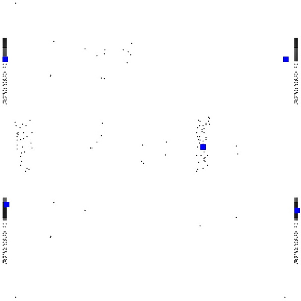
(a) InitialHeur

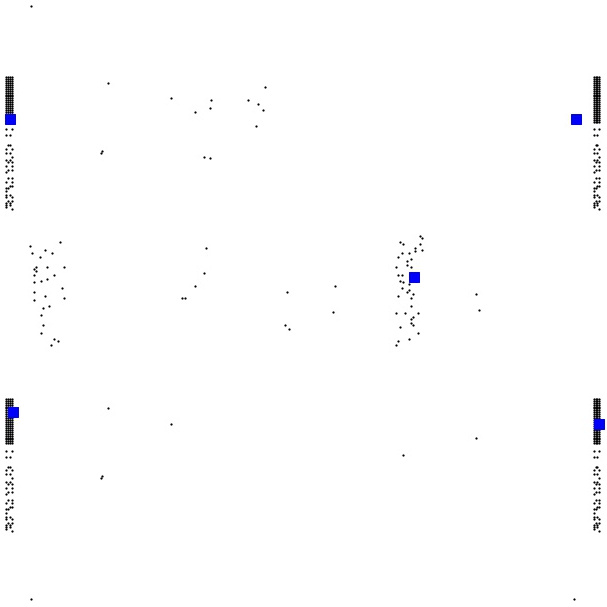
(b) Matheur

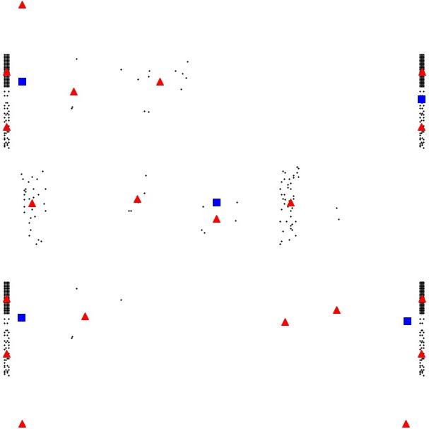
(c) KMEAN-20

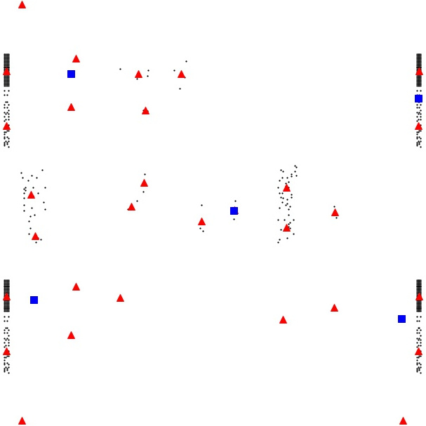
(d) KMEAN-30

Figure 1. Solutions for $n=654$ (Beasley, 1990), W, $p=5$, and $\ell_{1}$-norm

6. Conclusions

In this work, the Continuous Multifacility Monotone Ordered Median Problem is analyzed. This problem finds solutions in a continuous space and to solve it we have proposed two exact methods, namely a compact formulation and a branch-and-price procedure, using binary variables. Along the paper, we give full details of the branch-and-price algorithm and all its crucial steps: master problem, restricted relaxed master problem, pricing problem, initial pool of columns, feasibility, convergence, and branching.

Moreover, theoretic and empirical results have proven the utility of the obtained lower bound. Using that bound, we have tested the new proposed matheuristics. The decomposition-based heuristics have shown a very good performance on the computational experiments. For large-sized instances, it is worth highlighting that the exact procedure has improved the initial heuristic from 6.29% to 3.49% in average what in real applications could make a difference.

Among the extensive computational experiments and configurations of the problem, we highlight the usefulness of the branch-and-price approach for medium- to large-sized instances, but also the utility of the compact formulation and the aggregation-based heuristics for small values of $p$ or for some particular ordered weighted median functions.

Further research on the topic includes the design of similar branch-and-price approaches to other continuous facility location and clustering problems. Specifically, the application of set-partitioning column generation methods to hub location and covering problems with generalized upgrading (see, e.g., Blanco & Marín, 2019) where the index set for the $y$-variables must be adequately defined.

Appendix A Computational results for alternative $\ell_{\tau}$-norms

In this section, we show the results of our computational experiments for other $\ell_{\tau}$-norms, in particular, we have considered $\tau\in\{\frac{3}{2},2,3\}$. We have shown in Theorem 1 the general way to formulate the constraint for general values of $\tau$. In Table 7, we present the sets of constraints for the $\tau$ considered, forall $i\in I,j\in J,l\in\{1,\ldots,d\}$. Tables 8, 9, and 10 report the results.

$\ell_{\frac{3}{2}}$ $\ell_{2}$ $\ell_{3}$ $t_{ijl}\geq a_{il}-x_{jl},$ $t_{ijl}\geq a_{il}-x_{jl},$ $t_{ijl}\geq a_{il}-x_{jl},$ $t_{ijl}\geq-a_{il}+x_{jl},$ $t_{ijl}\geq-a_{il}+x_{jl},$ $t_{ijl}\geq-a_{il}+x_{jl},$ $z_{ij}\geq\displaystyle\sum_{l=1}^{d}\xi_{ijl},$ $z_{ij}^{2}\geq\displaystyle\sum_{l=1}^{d}t_{ijl}^{2},$ $z_{ij}\geq\displaystyle\sum_{l=1}^{d}\xi_{ijl}$ $t^{2}_{ijl}\leq\psi_{ijl}\xi_{ijl},$ $t_{ijl}^{2}\leq\psi_{ijl}z_{ij},$ $\psi^{2}_{ijl}\leq z_{ij}t_{ijl},$ $\psi^{2}_{ijl}\leq\xi_{ijl}t_{ijl},$

Table 7. Constraints for different values of $\tau$ to represent $\ell_{\tau}$-norms

$n$ type $p$ Time (#Unsolved) GAProot(%) GAP(%) Vars Nodes Memory (MB) Compact B&P Compact B&P Compact B&P Compact B&P Compact B&P Compact B&P 20 W 2 75.10 ( 0 ) 966.81 ( 0 ) 100.00 0.00 0.00 0.00 524 500 31161 1 187 25 5 — ( 5 ) 332.73 ( 0 ) 100.00 0.00 58.11 0.00 1270 397 2323815 1 11580 12 10 — ( 5 ) 152.66 ( 0 ) 100.00 0.00 97.34 0.00 2480 377 1280023 1 7438 10 C 2 0.70 ( 0 ) 520.73 ( 4 ) 100.00 21.46 0.00 17.11 524 13259 317 650 9 174 5 57.47 ( 0 ) 74.10 ( 4 ) 100.00 34.21 0.00 33.65 1270 1333 15338 302 44 13 10 3863.55 ( 1 ) 1270.00 ( 2 ) 100.00 18.56 2.45 17.81 2480 1638 1164203 1936 1159 15 K 2 6.23 ( 0 ) 1227.76 ( 2 ) 100.00 6.46 0.00 2.58 524 7247 3052 197 20 212 5 — ( 5 ) 824.52 ( 3 ) 100.00 10.90 27.82 6.21 1270 2719 3205611 1120 7563 57 10 — ( 5 ) 2409.37 ( 3 ) 100.00 17.66 96.76 8.78 2480 1235 1093174 3003 8496 24 D 2 63.65 ( 0 ) 724.11 ( 0 ) 100.00 0.00 0.00 0.00 524 437 31224 1 153 22 5 — ( 5 ) 284.21 ( 0 ) 100.00 0.00 65.95 0.00 1270 383 2204675 1 12441 11 10 — ( 5 ) 163.89 ( 0 ) 100.00 0.08 95.40 0.00 2480 370 1140802 3 9200 9 S 2 58.41 ( 0 ) 1040.72 ( 0 ) 100.00 0.00 0.00 0.00 524 519 25556 1 155 25 5 — ( 5 ) 423.48 ( 0 ) 100.00 0.11 59.03 0.00 1270 397 2398328 3 12161 12 10 — ( 5 ) 175.32 ( 0 ) 100.00 0.34 98.74 0.00 2480 383 878394 4 8683 10 A 2 16.20 ( 0 ) 2802.48 ( 1 ) 100.00 3.44 0.00 0.35 524 2987 5372 54 37 146 5 — ( 5 ) 2131.87 ( 2 ) 100.00 10.91 47.25 3.22 1270 2548 1996233 413 8655 69 10 — ( 5 ) 3440.13 ( 1 ) 100.00 11.84 99.32 2.01 2480 1288 705456 2001 7031 30 30 W 2 3007.98 ( 0 ) 854.86 ( 4 ) 86.97 19.38 0.00 19.38 784 852 1101778 1 2823 71 5 — ( 5 ) 3389.46 ( 3 ) 87.13 22.60 79.53 22.60 1900 845 744808 1 12424 47 10 — ( 5 ) 2960.90 ( 0 ) 89.05 0.00 88.07 0.00 3710 773 341608 2 3070 32 C 2 1.27 ( 0 ) 110.41 ( 4 ) 81.07 30.05 0.00 26.62 784 10754 416 190 15 137 5 311.13 ( 0 ) — ( 5 ) 81.71 45.91 0.00 44.26 1900 3340 57541 200 116 33 10 4.95 ( 4 ) — ( 5 ) 81.93 45.96 75.89 45.96 3710 1758 407909 231 1166 17 K 2 77.50 ( 0 ) 19.84 ( 4 ) 85.63 39.16 0.00 38.71 784 1708 28803 5 115 80 5 — ( 5 ) 20.48 ( 4 ) 85.80 18.37 66.83 17.99 1900 1986 956059 19 11102 61 10 — ( 5 ) 194.29 ( 4 ) 86.29 22.05 84.71 21.13 3710 1574 390091 234 2707 42 D 2 2441.14 ( 1 ) 300.79 ( 4 ) 86.55 22.86 2.74 22.86 784 918 1208553 1 3490 77 5 — ( 5 ) 4831.03 ( 2 ) 86.99 24.04 74.25 24.04 1900 841 798302 3 10071 48 10 — ( 5 ) 2546.68 ( 0 ) 87.46 0.05 86.29 0.00 3710 774 343890 2 4196 32 S 2 2363.80 ( 0 ) 470.41 ( 4 ) 86.86 32.35 0.00 32.35 784 895 822524 1 2187 72 5 — ( 5 ) 4534.78 ( 2 ) 86.78 18.98 76.88 18.98 1900 840 726885 1 10244 48 10 — ( 5 ) 2666.23 ( 0 ) 88.10 0.04 87.16 0.00 3710 776 410399 5 4551 31 A 2 327.89 ( 0 ) 93.44 ( 4 ) 85.31 49.21 0.00 49.18 784 1259 70967 2 365 104 5 — ( 5 ) 95.22 ( 4 ) 86.39 7.72 70.59 7.37 1900 1346 626210 9 8166 74 10 — ( 5 ) 169.25 ( 4 ) 86.14 13.71 84.74 10.99 3710 1487 307003 141 2647 54 40 W 2 — ( 5 ) — ( 5 ) 100.00 32.33 45.10 32.33 1044 1292 1282229 1 15092 131 5 — ( 5 ) — ( 5 ) 100.00 67.86 96.95 67.86 2530 1298 364182 1 8105 102 10 — ( 5 ) — ( 5 ) 100.00 92.83 100.00 92.83 4940 1339 165306 1 2712 83 C 2 4.22 ( 0 ) — ( 5 ) 100.00 44.51 0.00 44.51 1044 2468 1043 2 20 35 5 3879.78 ( 3 ) — ( 5 ) 100.00 77.56 41.01 77.56 2530 2525 606460 2 4626 27 10 — ( 5 ) — ( 5 ) 100.00 78.16 91.15 78.16 4940 2206 237096 13 883 22 K 2 2889.87 ( 0 ) — ( 5 ) 100.00 61.39 0.00 61.39 1044 2226 614033 1 2098 125 5 — ( 5 ) — ( 5 ) 100.00 83.30 92.54 83.30 2530 2213 451617 1 4187 94 10 — ( 5 ) — ( 5 ) 100.00 75.79 100.00 75.79 4940 2169 163856 3 1240 83 D 2 — ( 5 ) — ( 5 ) 100.00 32.13 40.95 32.13 1044 1529 1548255 1 11470 153 5 — ( 5 ) — ( 5 ) 100.00 68.37 99.29 68.37 2530 1310 360994 1 12324 99 10 — ( 5 ) — ( 5 ) 100.00 91.94 100.00 91.94 4940 1357 141565 1 4573 79 S 2 — ( 5 ) — ( 5 ) 100.00 30.53 42.63 30.53 1044 1443 1109568 1 14496 145 5 — ( 5 ) — ( 5 ) 100.00 72.37 98.23 72.37 2530 1299 358058 1 11144 97 10 — ( 5 ) — ( 5 ) 100.00 90.94 100.00 90.94 4940 1362 176603 1 2825 76 A 2 2886.85 ( 4 ) — ( 5 ) 100.00 61.20 14.49 61.20 1044 1876 1127650 1 3383 212 5 — ( 5 ) — ( 5 ) 100.00 82.57 93.62 82.57 2530 1656 402572 1 4383 134 10 — ( 5 ) — ( 5 ) 100.00 75.96 100.00 75.96 4940 1782 145643 1 2437 114 45 W 2 — ( 5 ) — ( 5 ) 100.00 34.65 46.87 34.65 1174 1462 974796 1 11024 145 5 — ( 5 ) — ( 5 ) 100.00 83.70 97.65 83.70 2845 1444 367765 1 3877 126 10 — ( 5 ) — ( 5 ) 100.00 100.00 100.00 100.00 5555 1522 122910 1 1081 101 C 2 6.63 ( 0 ) — ( 5 ) 100.00 57.24 0.00 57.24 1174 2438 1160 1 23 34 5 4337.92 ( 3 ) — ( 5 ) 100.00 84.59 49.89 84.59 2845 2696 467399 1 1217 33 10 — ( 5 ) — ( 5 ) 100.00 64.84 96.12 64.84 5555 2327 135558 3 578 24 K 2 6688.87 ( 4 ) — ( 5 ) 100.00 63.44 14.13 63.44 1174 2443 1718920 1 6733 142 5 — ( 5 ) — ( 5 ) 100.00 71.76 95.10 71.76 2845 2663 453635 1 3364 169 10 — ( 5 ) — ( 5 ) 100.00 91.29 99.70 91.29 5555 2231 158192 1 781 97 D 2 — ( 5 ) — ( 5 ) 100.00 30.83 48.64 30.83 1174 1508 933735 1 10637 153 5 — ( 5 ) — ( 5 ) 100.00 91.29 98.36 91.29 2845 1470 374986 1 5117 129 10 — ( 5 ) — ( 5 ) 100.00 100.00 100.00 100.00 5555 1528 159745 1 1184 106 S 2 — ( 5 ) — ( 5 ) 100.00 31.76 45.32 31.76 1174 1556 1059244 1 8872 160 5 — ( 5 ) — ( 5 ) 100.00 86.56 99.18 86.56 2845 1477 452467 1 4738 125 10 — ( 5 ) — ( 5 ) 100.00 100.00 100.00 100.00 5555 1522 131588 1 976 100 A 2 — ( 5 ) — ( 5 ) 100.00 60.42 25.43 60.42 1174 1992 861937 1 4928 221 5 — ( 5 ) — ( 5 ) 100.00 84.00 97.37 84.00 2845 1822 297805 1 4261 172 10 — ( 5 ) — ( 5 ) 100.00 93.77 100.00 93.77 5555 2008 141643 1 845 175 50 W 2 — ( 1 ) — ( 1 ) 100.00 36.39 57.48 36.39 1304 1749 759779 1 11084 186 5 — ( 1 ) — ( 1 ) 100.00 88.42 97.49 88.42 3160 1659 270228 1 3125 135 10 — ( 1 ) — ( 1 ) 100.00 100.00 100.00 100.00 6170 1777 122705 1 1843 127 C 2 6.06 ( 0 ) — ( 1 ) 100.00 57.05 0.00 57.05 1304 2813 879 1 28 36 5 — ( 1 ) — ( 1 ) 100.00 94.44 86.11 94.44 3160 2767 489141 1 1274 41 10 — ( 1 ) — ( 1 ) 100.00 66.91 100.00 66.91 6170 2678 117338 2 535 32 K 2 — ( 1 ) — ( 1 ) 100.00 66.85 22.51 66.85 1304 2554 1624297 1 9722 141 5 — ( 1 ) — ( 1 ) 100.00 95.48 92.64 95.48 3160 2458 501803 1 1496 132 10 — ( 1 ) — ( 1 ) 100.00 99.57 100.00 99.57 6170 2418 128940 1 669 115 D 2 — ( 1 ) — ( 1 ) 100.00 31.81 51.21 31.81 1304 1704 1059488 1 10438 182 5 — ( 1 ) — ( 1 ) 100.00 91.53 97.42 91.53 3160 1671 405884 1 1222 156 10 — ( 1 ) — ( 1 ) 100.00 100.00 100.00 100.00 6170 1710 156712 1 1360 127 S 2 — ( 1 ) — ( 1 ) 100.00 23.29 56.18 23.29 1304 2040 757576 1 10234 215 5 — ( 1 ) — ( 1 ) 100.00 46.71 98.40 46.71 3160 1772 404250 1 2374 166 10 — ( 1 ) — ( 1 ) 100.00 100.00 100.00 100.00 6170 1739 144453 1 764 131 A 2 — ( 1 ) — ( 1 ) 100.00 58.75 40.71 58.75 1304 2006 519352 1 6759 215 5 — ( 1 ) — ( 1 ) 100.00 86.23 95.15 86.23 3160 2175 396890 1 2119 208 10 — ( 1 ) — ( 1 ) 100.00 100.00 100.00 100.00 6170 2127 127758 1 672 183 Total Average: 1016.47 ( 282 ) 1438.77 ( 277 ) 96.64 44.54 59.19 43.82 2451 1902 628495 143 4813 85

Table 8. Results for Eilon et al. (1971) instances for $\ell_{\frac{3}{2}}$-norm

$n$ type $p$ Time (#Unsolved) GAProot(%) GAP(%) Vars Nodes Memory (MB) Compact B&P Compact B&P Compact B&P Compact B&P Compact B&P Compact B&P 20 W 2 26.03 ( 0 ) 24.22 ( 0 ) 100.00 0.00 0.00 0.00 204 2385 50632 1 41 120 5 — ( 5 ) 20.33 ( 0 ) 100.00 0.00 52.53 0.00 470 2504 8992191 1 15633 53 10 — ( 5 ) 9.15 ( 0 ) 100.00 0.00 89.75 0.00 880 2178 5306625 1 13982 28 C 2 0.16 ( 0 ) 757.86 ( 4 ) 100.00 18.45 0.00 10.76 204 45528 119 13798 4 962 5 16.30 ( 0 ) — ( 5 ) 100.00 32.78 0.00 21.37 470 7002 13102 7867 31 148 10 983.51 ( 0 ) 2223.12 ( 3 ) 100.00 27.39 0.00 10.97 880 3717 650055 9690 1569 75 K 2 5.03 ( 0 ) 1648.82 ( 1 ) 100.00 7.02 0.00 1.49 204 11126 6787 349 11 301 5 4231.23 ( 4 ) 2850.11 ( 2 ) 100.00 13.04 23.89 2.37 470 5627 8109266 1830 7136 117 10 — ( 5 ) 1822.27 ( 2 ) 100.00 16.01 85.45 6.61 880 2925 4227203 4287 11279 68 D 2 25.62 ( 0 ) 20.60 ( 0 ) 100.00 0.00 0.00 0.00 204 2365 45501 1 37 119 5 — ( 5 ) 15.53 ( 0 ) 100.00 0.00 50.45 0.00 470 2495 9156476 1 11659 52 10 — ( 5 ) 17.64 ( 0 ) 100.00 0.05 87.20 0.00 880 2175 5927899 2 15624 28 S 2 25.31 ( 0 ) 28.86 ( 0 ) 100.00 0.00 0.00 0.00 204 2445 42178 1 37 126 5 — ( 5 ) 49.89 ( 0 ) 100.00 0.03 49.72 0.00 470 2491 9117840 3 12277 53 10 — ( 5 ) 24.45 ( 0 ) 100.00 0.25 87.53 0.00 880 2183 5399238 4 15145 29 A 2 15.72 ( 0 ) 1663.90 ( 1 ) 100.00 3.21 0.00 0.17 204 6400 13975 133 19 288 5 — ( 5 ) 1603.15 ( 2 ) 100.00 9.93 36.09 1.74 470 5066 6284524 703 9720 138 10 — ( 5 ) 2420.97 ( 1 ) 100.00 15.86 87.63 0.94 880 2987 3478065 2125 11095 60 30 W 2 1214.67 ( 0 ) 264.29 ( 0 ) 86.79 0.00 0.00 0.00 304 3787 1814638 1 559 339 5 — ( 5 ) 80.27 ( 0 ) 86.91 0.00 72.61 0.00 700 2914 3104800 1 12866 107 10 — ( 5 ) 34.14 ( 0 ) 87.86 0.00 84.94 0.00 1310 2474 1626671 1 18935 54 C 2 0.43 ( 0 ) 104.99 ( 4 ) 81.07 14.80 0.00 11.58 304 45929 422 1794 6 643 5 76.89 ( 0 ) 503.59 ( 4 ) 81.71 27.87 0.00 20.17 700 8380 40315 1409 165 100 10 1.89 ( 4 ) — ( 5 ) 81.93 38.05 41.89 33.92 1310 4996 2709802 2978 4156 69 K 2 54.31 ( 0 ) 744.55 ( 4 ) 85.50 6.60 0.00 6.45 304 7743 62564 44 58 368 5 — ( 5 ) 5040.71 ( 4 ) 86.00 11.54 67.36 8.59 700 5932 2838928 295 15993 170 10 — ( 5 ) — ( 5 ) 87.68 17.84 83.29 13.27 1310 4040 1799130 1270 12831 88 D 2 1247.78 ( 0 ) 222.14 ( 0 ) 86.38 0.00 0.00 0.00 304 3810 1731910 1 529 335 5 — ( 5 ) 139.30 ( 0 ) 86.94 0.00 73.46 0.00 700 2939 2824067 1 12906 108 10 — ( 5 ) 38.85 ( 0 ) 87.51 0.00 85.28 0.00 1310 2480 1519282 1 16694 55 S 2 1271.98 ( 0 ) 186.78 ( 0 ) 86.69 0.00 0.00 0.00 304 3699 1631950 1 518 324 5 — ( 5 ) 540.52 ( 0 ) 87.12 0.02 73.42 0.00 700 2905 3042832 3 13666 109 10 — ( 5 ) 94.57 ( 0 ) 87.66 0.08 84.50 0.00 1310 2465 1569091 2 13710 55 A 2 220.34 ( 0 ) 3254.28 ( 3 ) 85.20 2.15 0.00 1.69 304 4997 136052 16 110 403 5 — ( 5 ) 1745.13 ( 4 ) 86.59 5.37 71.23 3.06 700 4216 1909608 51 10892 174 10 — ( 5 ) 1207.09 ( 4 ) 86.97 11.27 83.28 6.38 1310 3735 1103129 465 10680 106 40 W 2 — ( 5 ) 252.49 ( 0 ) 100.00 0.00 31.03 0.00 404 6365 7312331 1 5864 817 5 — ( 5 ) 364.88 ( 0 ) 100.00 0.00 94.01 0.00 930 4168 1925927 1 11549 234 10 — ( 5 ) 355.67 ( 0 ) 100.00 0.00 99.63 0.00 1740 3922 862095 1 8294 120 C 2 1.55 ( 0 ) — ( 5 ) 100.00 23.26 0.00 22.73 404 29032 1164 419 9 448 5 594.78 ( 0 ) — ( 5 ) 100.00 36.17 0.00 35.69 930 5983 271138 92 862 57 10 4207.08 ( 1 ) — ( 5 ) 100.00 37.29 11.40 35.81 1740 4780 1357589 266 5116 40 K 2 719.29 ( 0 ) — ( 5 ) 100.00 8.69 0.00 8.69 404 5651 701127 4 429 412 5 — ( 5 ) — ( 5 ) 100.00 16.32 89.79 16.31 930 4724 1771444 4 11673 171 10 — ( 5 ) — ( 5 ) 100.00 16.50 99.43 16.47 1740 4836 700210 44 13117 100 D 2 — ( 5 ) 259.07 ( 0 ) 100.00 0.00 30.59 0.00 404 6694 6885185 1 7289 865 5 — ( 5 ) 485.52 ( 0 ) 100.00 0.00 94.27 0.00 930 4240 2040736 1 9260 238 10 — ( 5 ) 473.11 ( 0 ) 100.00 0.01 99.90 0.00 1740 3891 692838 1 10352 119 S 2 — ( 5 ) 691.25 ( 0 ) 100.00 0.02 29.89 0.00 404 6224 6075474 1 5159 806 5 — ( 5 ) 244.29 ( 0 ) 100.00 0.00 94.33 0.00 930 4120 2196020 1 11994 230 10 — ( 5 ) 1223.93 ( 0 ) 100.00 0.07 99.90 0.00 1740 3910 925128 3 11056 120 A 2 3347.72 ( 4 ) — ( 5 ) 100.00 4.09 9.28 4.09 404 5760 2823594 2 1885 763 5 — ( 5 ) — ( 5 ) 100.00 9.56 91.43 9.08 930 4410 1346465 5 6365 258 10 — ( 5 ) — ( 5 ) 100.00 9.54 99.86 8.60 1740 4404 677970 41 9029 141 45 W 2 — ( 5 ) 388.20 ( 0 ) 100.00 0.00 41.73 0.00 454 9960 4536228 1 6272 1570 5 — ( 5 ) 207.18 ( 0 ) 100.00 0.00 96.23 0.00 1045 4741 1544401 1 10363 360 10 — ( 5 ) 282.84 ( 0 ) 100.00 0.00 100.00 0.00 1955 4318 494940 1 10023 172 C 2 2.49 ( 0 ) — ( 5 ) 100.00 22.33 0.00 22.32 454 4517 1618 6 13 67 5 398.50 ( 0 ) — ( 5 ) 100.00 35.75 0.00 35.62 1045 4850 162356 10 453 46 10 — ( 5 ) — ( 5 ) 100.00 35.00 76.29 34.76 1955 4710 1628650 35 5534 36 K 2 5287.03 ( 2 ) — ( 5 ) 100.00 12.13 5.66 12.12 454 6140 4935475 3 2537 535 5 — ( 5 ) — ( 5 ) 100.00 17.38 93.84 17.36 1045 5116 2086094 4 9338 226 10 — ( 5 ) — ( 5 ) 100.00 14.67 100.00 14.67 1955 4781 618710 5 11268 120 D 2 — ( 5 ) 358.37 ( 0 ) 100.00 0.00 40.50 0.00 454 9220 4961123 1 5740 1483 5 — ( 5 ) 207.01 ( 0 ) 100.00 0.00 96.12 0.00 1045 4756 1837767 1 8596 363 10 — ( 5 ) 483.48 ( 0 ) 100.00 0.00 100.00 0.00 1955 4310 486390 1 9703 172 S 2 — ( 5 ) 370.88 ( 0 ) 100.00 0.00 40.04 0.00 454 9566 4705056 1 5430 1507 5 — ( 5 ) 1332.07 ( 0 ) 100.00 0.20 95.75 0.00 1045 4809 2080272 4 10194 370 10 — ( 5 ) 1487.71 ( 0 ) 100.00 0.02 99.90 0.00 1955 4315 659990 3 10857 173 A 2 — ( 5 ) — ( 5 ) 100.00 6.72 25.73 6.26 454 6957 2069919 4 3364 1078 5 — ( 5 ) — ( 5 ) 100.00 11.97 91.39 11.12 1045 4895 1615563 6 3655 373 10 — ( 5 ) — ( 5 ) 100.00 7.59 100.00 7.46 1955 4486 483721 6 8786 172 50 W 2 — ( 1 ) 456.01 ( 0 ) 100.00 0.00 48.21 0.00 504 10414 4777385 1 6240 2007 5 — ( 1 ) 615.74 ( 0 ) 100.00 0.03 96.50 0.00 1160 5458 1930033 3 6233 470 10 — ( 1 ) 204.96 ( 0 ) 100.00 0.00 100.00 0.00 2170 4971 355938 1 7946 232 C 2 4.78 ( 0 ) — ( 1 ) 100.00 22.61 0.00 22.61 504 4342 2935 2 17 59 5 — ( 1 ) — ( 1 ) 100.00 34.42 67.17 34.37 1160 5142 2940681 4 5728 51 10 — ( 1 ) — ( 1 ) 100.00 40.27 83.64 40.21 2170 5198 1333733 18 3970 41 K 2 — ( 1 ) — ( 1 ) 100.00 11.24 18.49 11.24 504 6665 4998109 3 3635 673 5 — ( 1 ) — ( 1 ) 100.00 17.43 91.41 17.43 1160 5674 3154623 3 5249 284 10 — ( 1 ) — ( 1 ) 100.00 14.01 100.00 13.91 2170 5463 567705 7 10827 156 D 2 — ( 1 ) 405.36 ( 0 ) 100.00 0.00 47.33 0.00 504 9675 4367022 1 6329 1789 5 — ( 1 ) 209.77 ( 0 ) 100.00 0.00 94.73 0.00 1160 5302 2598004 1 4692 469 10 — ( 1 ) 605.10 ( 0 ) 100.00 0.00 100.00 0.00 2170 5000 548086 1 7504 233 S 2 — ( 1 ) 451.37 ( 0 ) 100.00 0.00 48.39 0.00 504 10286 3512436 1 6039 1986 5 — ( 1 ) 815.35 ( 0 ) 100.00 0.07 96.27 0.00 1160 5236 3055646 3 6241 459 10 — ( 1 ) 204.63 ( 0 ) 100.00 0.01 100.00 0.01 2170 4900 386889 1 9984 231 A 2 — ( 1 ) — ( 1 ) 100.00 5.95 32.08 5.36 504 8326 1790159 4 2035 1513 5 — ( 1 ) — ( 1 ) 100.00 12.91 91.62 11.92 1160 5559 1874166 7 3311 483 10 — ( 1 ) — ( 1 ) 100.00 7.13 100.00 6.88 2170 5089 462300 9 10198 231 Total Average: 673.68 ( 267 ) 557.40 ( 157 ) 96.65 8.44 53.08 6.79 886 6179 2347788 663 7186 310

Table 9. Results for Eilon et al. (1971) instances for $\ell_{2}$-norm

$n$ type $p$ Time (#Unsolved) GAProot(%) GAP(%) Vars Nodes Memory (MB) Compact B&P Compact B&P Compact B&P Compact B&P Compact B&P Compact B&P 20 W 2 151.03 ( 0 ) 743.17 ( 0 ) 100.00 0.00 0.00 0.00 524 471 56126 1 418 24 5 — ( 5 ) 267.56 ( 0 ) 100.00 0.00 62.95 0.00 1270 415 2700255 1 13112 14 10 — ( 5 ) 133.91 ( 0 ) 100.00 0.00 98.54 0.00 2480 406 1259405 1 13418 13 C 2 0.91 ( 0 ) — ( 5 ) 100.00 30.56 0.00 29.19 524 9181 507 417 11 121 5 71.86 ( 0 ) — ( 5 ) 100.00 35.58 0.00 30.56 1270 3061 17235 1473 62 32 10 2142.39 ( 0 ) — ( 5 ) 100.00 47.17 0.00 47.00 2480 912 261767 553 879 8 K 2 16.05 ( 0 ) 5363.15 ( 2 ) 100.00 9.14 0.00 2.07 524 12397 7592 424 40 352 5 — ( 5 ) 2946.11 ( 3 ) 100.00 14.87 38.13 5.02 1270 3466 2839547 1556 8104 75 10 — ( 5 ) 3206.51 ( 2 ) 100.00 8.25 93.62 5.18 2480 1348 1021924 2630 6013 23 D 2 125.29 ( 0 ) 810.43 ( 0 ) 100.00 0.00 0.00 0.00 524 498 53138 1 300 26 5 — ( 5 ) 230.99 ( 0 ) 100.00 0.00 60.85 0.00 1270 382 2732256 1 12124 11 10 — ( 5 ) 112.30 ( 0 ) 100.00 0.09 99.24 0.00 2480 377 1083407 2 11367 10 S 2 104.35 ( 0 ) 973.36 ( 0 ) 100.00 0.05 0.00 0.00 524 530 45754 1 239 27 5 — ( 5 ) 255.50 ( 0 ) 100.00 0.11 64.54 0.00 1270 398 2470849 2 10763 12 10 — ( 5 ) 125.04 ( 0 ) 100.00 0.26 99.51 0.00 2480 378 1131966 4 11380 10 A 2 33.54 ( 0 ) 2705.24 ( 1 ) 100.00 4.22 0.00 0.15 524 3049 11374 71 74 150 5 — ( 5 ) 1648.71 ( 2 ) 100.00 8.18 42.12 1.90 1270 2262 2117999 329 6961 64 10 — ( 5 ) 4194.46 ( 1 ) 100.00 13.35 99.33 1.41 2480 1216 842028 2054 8107 29 30 W 2 2404.31 ( 4 ) 435.00 ( 4 ) 86.64 14.53 12.54 14.53 784 843 2130171 1 10112 65 5 — ( 5 ) 3934.80 ( 2 ) 86.35 5.57 77.53 5.57 1900 860 830494 1 12706 48 10 — ( 5 ) 2479.98 ( 0 ) 86.89 0.03 86.14 0.00 3710 816 306492 3 4764 37 C 2 2.30 ( 0 ) 1631.39 ( 4 ) 81.07 29.54 0.00 29.53 784 7137 675 7559 17 94 5 571.24 ( 0 ) 2360.18 ( 4 ) 81.71 48.42 0.00 46.18 1900 2388 71418 386 212 27 10 8.07 ( 4 ) 1801.17 ( 4 ) 81.93 48.01 71.16 47.51 3710 1236 316323 33 1003 10 K 2 211.31 ( 0 ) 17.36 ( 4 ) 85.39 24.11 0.00 23.96 784 1808 86793 7 303 81 5 — ( 5 ) 27.59 ( 4 ) 86.11 14.05 63.23 13.64 1900 1707 1143862 12 9716 52 10 — ( 5 ) 34.09 ( 4 ) 85.92 22.77 85.05 22.13 3710 1409 365197 168 4413 35 D 2 4446.26 ( 3 ) 3777.09 ( 3 ) 86.24 18.03 10.14 18.03 784 946 2197143 1 9689 71 5 — ( 5 ) 3574.66 ( 2 ) 86.38 9.19 74.99 9.19 1900 853 958686 1 12995 45 10 — ( 5 ) 2472.72 ( 0 ) 86.60 0.06 85.43 0.00 3710 796 375899 3 5968 35 S 2 3256.59 ( 3 ) 305.27 ( 4 ) 86.54 17.51 9.82 17.51 784 850 1889060 1 8632 70 5 — ( 5 ) 3697.87 ( 1 ) 86.19 1.29 78.49 1.23 1900 760 873284 2 12851 40 10 — ( 5 ) 2525.29 ( 0 ) 87.92 0.12 87.51 0.00 3710 791 351574 4 4490 32 A 2 1365.87 ( 0 ) 61.55 ( 4 ) 85.11 21.30 0.00 21.04 784 1141 327100 3 1255 96 5 — ( 5 ) 11.83 ( 4 ) 85.51 7.43 72.18 6.75 1900 1251 643473 8 9003 67 10 — ( 5 ) 100.35 ( 4 ) 85.84 15.80 84.79 13.75 3710 1385 306764 101 4475 51 40 W 2 — ( 5 ) — ( 5 ) 100.00 26.96 51.29 26.96 1044 1248 1344963 1 16445 121 5 — ( 5 ) — ( 5 ) 100.00 83.14 95.28 83.14 2530 1267 482105 1 5041 104 10 — ( 5 ) — ( 5 ) 100.00 92.94 100.00 92.94 4940 1350 188692 1 3381 85 C 2 6.66 ( 0 ) — ( 5 ) 100.00 38.00 0.00 37.95 1044 2502 1762 5 22 37 5 2658.74 ( 2 ) — ( 5 ) 100.00 81.92 39.02 81.92 2530 2235 434526 1 3523 25 10 — ( 5 ) — ( 5 ) 100.00 75.34 100.00 75.34 4940 1921 349858 12 1348 18 K 2 4990.55 ( 1 ) — ( 5 ) 100.00 50.04 3.02 50.04 1044 2202 1651655 1 5136 113 5 — ( 5 ) — ( 5 ) 100.00 74.12 97.64 74.12 2530 2018 479613 1 7167 86 10 — ( 5 ) — ( 5 ) 100.00 69.68 100.00 69.68 4940 1934 210396 3 2563 72 D 2 — ( 5 ) — ( 5 ) 100.00 20.20 42.95 20.20 1044 1247 1505294 1 12264 125 5 — ( 5 ) — ( 5 ) 100.00 89.82 98.91 89.82 2530 1248 463628 1 8186 98 10 — ( 5 ) — ( 5 ) 100.00 90.59 100.00 90.59 4940 1350 153036 1 5215 87 S 2 — ( 5 ) — ( 5 ) 100.00 25.20 43.94 25.20 1044 1323 1360254 1 12167 126 5 — ( 5 ) — ( 5 ) 100.00 70.38 96.48 70.38 2530 1294 462667 1 6780 91 10 — ( 5 ) — ( 5 ) 100.00 84.09 100.00 84.09 4940 1334 139121 1 6489 81 A 2 — ( 5 ) — ( 5 ) 100.00 24.46 22.07 24.46 1044 1810 1460678 1 5826 191 5 — ( 5 ) — ( 5 ) 100.00 62.67 99.14 62.67 2530 1646 345643 1 7108 134 10 — ( 5 ) — ( 5 ) 100.00 85.25 100.00 85.25 4940 1767 155190 1 3426 113 45 W 2 — ( 5 ) — ( 5 ) 100.00 26.30 54.64 26.30 1174 1398 1133697 1 11416 134 5 — ( 5 ) — ( 5 ) 100.00 92.43 99.51 92.43 2845 1413 401143 1 5947 113 10 — ( 5 ) — ( 5 ) 100.00 100.00 100.00 100.00 5555 1469 153297 1 2343 104 C 2 6.40 ( 0 ) — ( 5 ) 100.00 46.67 0.00 46.67 1174 2326 1132 2 24 34 5 5003.88 ( 3 ) — ( 5 ) 100.00 75.71 60.00 75.71 2845 2532 500043 1 5891 29 10 — ( 5 ) — ( 5 ) 100.00 75.66 100.00 75.64 5555 2236 171358 7 722 22 K 2 — ( 5 ) — ( 5 ) 100.00 44.43 28.39 44.43 1174 2477 1611616 1 11832 146 5 — ( 5 ) — ( 5 ) 100.00 80.52 99.07 80.52 2845 2482 426670 1 6214 157 10 — ( 5 ) — ( 5 ) 100.00 84.97 100.00 84.97 5555 2165 160867 1 1944 90 D 2 — ( 5 ) — ( 5 ) 100.00 24.77 54.89 24.77 1174 1406 1171833 1 12252 135 5 — ( 5 ) — ( 5 ) 100.00 98.15 98.67 98.15 2845 1412 424560 1 4188 113 10 — ( 5 ) — ( 5 ) 100.00 100.00 100.00 100.00 5555 1466 152963 1 2822 104 S 2 — ( 5 ) — ( 5 ) 100.00 23.69 56.00 23.69 1174 1479 1069851 1 11291 141 5 — ( 5 ) — ( 5 ) 100.00 72.98 99.95 72.98 2845 1450 514193 1 5809 107 10 — ( 5 ) — ( 5 ) 100.00 100.00 100.00 100.00 5555 1467 159205 1 2847 101 A 2 — ( 5 ) — ( 5 ) 100.00 24.73 37.56 24.73 1174 1731 695531 1 6228 178 5 — ( 5 ) — ( 5 ) 100.00 65.14 97.05 65.14 2845 1800 295359 1 4504 160 10 — ( 5 ) — ( 5 ) 100.00 95.05 100.00 95.05 5555 2027 131122 1 1477 172 50 W 2 — ( 1 ) — ( 1 ) 100.00 75.57 61.16 75.57 1304 1616 1047768 1 11081 161 5 — ( 1 ) — ( 1 ) 100.00 99.83 100.00 99.83 3160 1623 406553 1 2969 141 10 — ( 1 ) — ( 1 ) 100.00 100.00 100.00 100.00 6170 1709 186637 1 934 128 C 2 11.71 ( 0 ) — ( 1 ) 100.00 62.36 0.00 62.36 1304 2575 2112 1 38 37 5 — ( 1 ) — ( 1 ) 100.00 90.14 87.76 90.14 3160 2577 540242 1 1441 34 10 — ( 1 ) — ( 1 ) 100.00 99.12 100.00 99.12 6170 2587 112265 1 572 26 K 2 — ( 1 ) — ( 1 ) 100.00 36.29 46.27 36.29 1304 2810 957166 1 10628 164 5 — ( 1 ) — ( 1 ) 100.00 91.13 98.89 91.13 3160 2450 434558 1 4069 127 10 — ( 1 ) — ( 1 ) 100.00 90.03 100.00 90.03 6170 2410 142538 1 1231 108 D 2 — ( 1 ) — ( 1 ) 100.00 31.05 63.12 31.05 1304 1666 878351 1 10528 162 5 — ( 1 ) — ( 1 ) 100.00 74.10 100.00 74.10 3160 1695 285611 1 4410 134 10 — ( 1 ) — ( 1 ) 100.00 100.00 100.00 100.00 6170 1777 83410 1 545 129 S 2 — ( 1 ) — ( 1 ) 100.00 36.71 60.33 36.71 1304 1577 983547 1 10718 148 5 — ( 1 ) — ( 1 ) 100.00 94.34 99.55 94.34 3160 1635 583530 1 2230 129 10 — ( 1 ) — ( 1 ) 100.00 100.00 100.00 100.00 6170 1737 153870 1 775 135 A 2 — ( 1 ) — ( 1 ) 100.00 24.67 48.59 24.67 1304 2258 514472 1 5470 226 5 — ( 1 ) — ( 1 ) 100.00 75.58 100.00 75.58 3160 1998 403520 1 2368 182 10 — ( 1 ) — ( 1 ) 100.00 91.23 100.00 91.23 6170 2051 117660 1 1968 170 Total Average: 928.16 ( 292 ) 1680.95 ( 276 ) 96.54 41.27 61.20 40.52 2451 1819 711082 237 5823 82

Table 10. Results for Eilon et al. (1971) instances for $\ell_{3}$-norm

References

- Albornoz & Zamora (2021) Albornoz, V. M., & Zamora, G. E. (2021). Decomposition-based heuristic for the zoning and crop planning problem with adjacency constraints. Top, 29(1), 248–265.
- Avella et al. (2007) Avella, P., Sassano A., & Vasil’ev, I. (2007). Computational study of large-scale -Median problems. Mathematical Programming Series A, 109, 89–114.
- Barnhart et al. (1998) Barnhart, C., Johnson, E. L., Nemhauser, G. L., Savelsbergh M. W. P., & Vance, P. H. (1998). Branch-and-price: column generation for solving huge integer programs. Operations Research, 46(3), 316–319.
- Beasley (1985) Beasley J. E. (1985). A note on solving large p-median problems. European Journal of Operational Research, 21(2), 270–273.
- Beasley (1990) Beasley J. E. (1990). OR-Library: Distributing Test Problems by Electronic Mail. Journal of the Operational Research Society, 41, 1069–1072. http://people.brunel.ac.uk/~mastjjb/jeb/info.html
- Benati et al. (2021) Benati, S., Ponce, D., Puerto, J., & Rodríguez-Chía, A. M. (2021). A branch-and-price procedure for clustering data that are graph connected. European Journal of Operational Research. https://doi.org/10.1016/j.ejor.2021.05.043
- Blanco (2019) Blanco, V. (2019). Ordered p-median problems with neighbourhoods. Computational Optimization and Applications, 73(2), 603-645.
- Blanco et al. (2014) Blanco, V., ElHaj BenAli, S., & Puerto, J., (2014). Revisiting several problems and algorithms in continuous location. with -norms. Computational Optimization and Applications, 58(3), 563–595.
- Blanco & Gázquez (2021) Blanco, V., & Gázquez, R. (2021). Continuous maximal covering location problems with interconnected facilities. Computers & Operations Research, 132, 105310.
- Blanco et al. (2021) Blanco, V., Japón, A., Ponce, D., & Puerto, J. (2021). On the multisource hyperplanes location problem to fitting set of points. Computers & Operations Research, 128, 105124.
- Blanco & Marín (2019) Blanco, V., & Marín, A. (2019). Upgrading nodes in tree-shaped hub location. Computers & Operations Research, 102, 75-90.
- Blanco et al. (2016) Blanco, V., Puerto, J., & ElHaj BenAli, S. (2016). Continuous multifacility ordered median location problems. European Journal of Operational Research, 250(1), 56–64.
- Blanco et al. (2017) Blanco, V., Puerto, J., & Ponce, D. (2017). Continuous location under the effect of refraction. Mathematical Programming, 161(1), 33–72.
- Blanco et al. (2018) Blanco, V., Puerto, J., & Salmerón, R. (2018). Locating hyperplanes to fitting set of points: A general framework. Computers & Operations Research, 95, 172–193.
- Brimberg (1995) Brimberg, J. (1995). The Fermat–Weber location problem revisited. Mathematical Programming, 71, 71–76.
- Carrizosa et al. (1995) Carrizosa E., Conde, E., Muñoz, M. & Puerto, J. (1995) The generalized Weber problem with expected distances. RAIRO-Operations Research, 29, 35–57.
- Carrizosa et al. (1998) Carrizosa, E., Muñoz-Márquez, M., & Puerto, J. (1998). The Weber problem with regional demand. European Journal of Operational Research, 104(2), 358–365.
- Chandrasekaran & Tamir (1989) Chandrasekaran, R., & Tamir, A. (1989). Open questions concerning Weiszfeld’s algorithm for the Fermat-Weber location problem. Mathematical Programming, 44, 293–295.
- Current & Schilling (1990) Current, J.R., & Schilling, D.A. (1990). Analysis of errors due to demand data aggregation in the set covering and maximal covering location problems. Geographical Analysis, 22(2), 116–126.
- Daskin et al. (1989) Daskin, M. S., Haghani, A. E., Khanal, M., & Malandraki, C. (1989). Aggregation effects in maximum covering models. Annals of Operations Research, 18(1), 113–139.
- Deleplanque et al. (2020) Deleplanque, S., Labbé, M., Ponce, D., & Puerto, J. (2020). A Branch-Price-and-Cut Procedure for the Discrete Ordered Median Problem. INFORMS Journal on Computing, 32(3), 582–599.
- Desrosiers & Lübecke (2005) Desrosiers, J., & Lübecke, M. (2005). A primer in column generation. In G. Desaulniers, J. Desrosiers & M. M. Salomon (Eds.), Column Generation (pp. 1–32). Springer, Boston.
- Drezner & Hamacher (2002) Drezner, Z., & Hamacher, H. W. (Eds.). (2002). Facility Location: Applications and Theory. Springer-Verlag Berlin Heidelberg.
- Eilon et al. (1971) Eilon, S., Watson-Gandy, C. D. T., & Christofides, N. (1971). Distribution management: mathematical modeling and practical analysis. London: Griffin.
- Elloumi et al. (2004) Elloumi, S., Labbé, M., & Pochet, Y. (2004). A New Formulation and Resolution Method for the p-Center Problem. INFORMS Journal on Computing, 16(1), 84–94.
- Espejo et al. (2009) Espejo, I., Marín, A., Puerto, J., & Rodríguez-Chía, A. M. (2009). A comparison of formulations and solution methods for the Minimum-Envy Location Problem. Computers & Operations Research, 36(6), 1966–1981.
- Espejo et al. (2021) Espejo, I., Puerto, J., & Rodriguez-Chia, A. M. (2021). A comparative study of different formulations for the Capacitated Discrete Ordered Median Problem. Computers & Operations Research, 125, 105067.
- Fekete et al. (2005) Fekete, S. P., Mitchell, J. S. B., & Beurer, K. (2005). On the Continuous Fermat-Weber Problem. Operations Research, 53(1), 61–76.
- Fernández et al. (2014) Fernández, E. Pozo, M. A., & Puerto, J. (2014). Ordered Weighted Average Combinatorial Optimization: Formulations and their properties. Discrete Applied Mathematics, 169(31), 97–118.
- Gamrath et al. (2020) Gamrath, G., Anderson, D., Bestuzheva, K., et al. (2020) The SCIP Optimization Suite 7.0. ZIB-Report 20-10, Zuse Institute Berlin. http://nbn-resolving.de/urn:nbn:de:0297-zib-78023
- García et al. (2010) García, S., Labbé, M., & Marín, A. (2010). Solving Large p-Median Problems with a Radius Formulation. INFORMS Journal on Computing, 23(4), 546–556.
- Geoffrion (1977) Geoffrion, A. M. (1977). Objective function approximations in mathematical programming. Mathematical Programming, 13(1), 23–37.
- Irawan (2016) Irawan, C. A. (2016). Aggregation and non aggregation techniques for large facility location problems-a survey. Yugoslav Journal of Operations Research, 25(3).
- Krau (1997) Krau, S. (1997). Extensions du probléme de Weber (Ph. D. Dissertation, École Polytechnique de Montréal, Montréal, Canada).
- Labbé et al. (2017) Labbé, M., Ponce D., & Puerto J. (2017) A Comparative Study of Formulations and Solution Methods for the Discrete Ordered -Median Problem. Computers & Operations Research, 78, 230–242.
- Laporte et al. (2015) Laporte, G., Nickel, S., & Saldanha da Gama, F. (Eds.). (2015). Location Science. Springer International Publishing.
- Mallozi et al. (2019) Mallozzi, L., Puerto, J., & Rodríguez-Madrena, M. (2019). On location-allocation problems for dimensional facilities. Journal of Optimization Theory and Applications, 182(2), 730–767.
- Manzour-al-Ajdad et al. (2012) Manzour-al-Ajdad, S. M. H., Torabi, S. A., & Eshghi, K. (2012). Single-Source Capacitated Multi-Facility Weber Problem—An iterative two phase heuristic algorithm. Computers & Operations Research, 39(7), 1465–1476.
- Marín et al. (2009) Marín, A., Nickel, S., Puerto, J., & Velten, S. (2009). A Flexible Model and Efficient Solution Strategies for Discrete Location Problems. Discrete Applied Mathematics, 157, 1128-1145.
- Marín et al. (2010) Marín, A., Nickel, S., & Velten, S. (2010). An extended covering model for flexible discrete and equity location problems. Mathematical Methods of Operations Research, 71, 125-163.
- Marín et al. (2020) Marín A., Ponce, D., & Puerto, J. (2020). A fresh view on the Discrete Ordered Median Problem based on partial monotonicity. European Journal of Operational Research, 286, 839–848.
- du Merle et al. (1999) du Merle, O., Villenueve, D., Desrosiers, J., & Hansen, P. (1999). Stabilized column generation. Discrete Mathematics, 194, 229–237.
- du Merle & Vial (2002) du Merle, O., & Vial, J. (2002). Proximal ACCPM, a cutting plane method for column generation and Lagrangean relaxation: application to the -median problem. Tech. rep., HEC Genève, Université de Genève.
- Nickel & Puerto (2005) Nickel, S., & Puerto, J. (2005). Location Theory: A Unified Approach. Springer Verlag.
- Nickel et al. (2003) Nickel, S., Puerto, J., & Rodríguez-Chía, A. M. (2003). An Approach to Location Models Involving Sets as Existing Facilities. Mathematics of Operations Research, 28(4), 693–715.
- Puerto (2020) Puerto, J. (2020). An exact completely positive programming formulation for the Discrete Ordered Median Problem: An extended version. Journal of Global Optimization, 77(2), 341–359.
- Puerto et al. (2013) Puerto, J., Ramos, A. B., & Rodríguez-Chía, A. M. (2013). A specialized Branch & Bound & Cut for Single-Allocation Ordered Median Hub Location problems. Discrete Applied Mathematics, 161, 2624–2624.
- Puerto & Rodríguez-Chía (2011) Puerto, J., & Rodríguez-Chía, A. M. (2011). On the structure of the solution set for the single facility location problem with average distances. Mathematical Programming, 128, 373–401.
- Puerto & Tamir (2005) Puerto, J., & Tamir, A. (2005). Locating tree-shaped facilities using the ordered median objective. Mathematical Programming, 102, 313–338.
- Righini & Zaniboni (2007) Righini, G., & Zaniboni, L. (2007). A branch-and-price algorithm for the multi-source Weber problem. International Journal of Operational Research, 2(2), 188–207.
- Rosing (1992) Rosing, K. E. (1992). An optimal method for solving the (generalized) multi-Weber problem. European Journal of Operational Research, 58(3), 414–426.
- Ryan & Foster (1981) Ryan, D. M., & Foster, B. A. (1981). An integer programming approach to scheduling. In A. Wren (Ed.), Computer Scheduling of Public Transport (pp. 269–280). North-Holland, Amsterdan.
- Sakai et al. (2003) Sakai, S., Togasaki, M., & Yamazaki, K. (2003). A note on greedy algorithms for the maximum weighted independent set problem. Discrete Applied Mathematics, 126(2), 313–322.
- Sherali & Nordai (1988) Sherali, H. D., & Nordai, F. L. (1988). Np-hard, capacitated, balanced p-median problems on a chain graph with a continuum of link demands. Mathematics of Operation Research, 13(1), 32–49.
- Valero-Franco et al. (2013) Valero-Franco, C., Rodríguez-Chía, A. M., & Espejo, I. (2013). Accelerating convergence in minisum location problem with norms. Computers & Operations Research, 40(11), 2770–2785.
- Venkateshan & Mathur (2015) Venkateshan, P., & Mathur, K. (2015). A Heuristic for the Multisource Weber Problem with Service Level Constraints. Transportation Science, 49(3), 472-483.
- Ward & Wendell (1985) Ward, J. E., & Wendell, R. E. (1985). Using block norms for location modeling. Operations Research, 33(5), 1074–1090.
- Weiszfeld (1937) Weiszfeld, E. (1937). Sur le point par lequel la somme des distances den points donnés est minimum. Tohoku Mathematics Journal, 43, 355–386.