Adaptive interface-Mesh un-Refinement (AiMuR) based Sharp-Interface Level-Set-Method for Two-Phase Flow

Abstract

Adaptive interface-Mesh un-Refinement (AiMuR) based Sharp-Interface Level-Set-Method (SI-LSM) is proposed for both uniform and non-uniform Cartesian-Grid. The AiMuR involves interface location based dynamic un-refinement (with merging of the four control volumes) of the Cartesian grid away from the interface. The un-refinement is proposed for the interface solver only. A detailed numerical methodology is presented for the AiMuR and ghost-fluid method based SI-LSM. Advantage of the novel as compared to the traditional SI-LSM is demonstrated with a detailed qualitative as well as quantitative performance study, involving the SI-LSMs on both coarse grid and fine grid, for three sufficiently different two-phase flow problems: dam break, breakup of a liquid jet and drop coalescence. A superior performance of AiMuR based SI-LSM is demonstrated - the AiMuR on a coarser non-uniform grid ($NU_{c}^{AiMuR}$) is almost as accurate as the traditional SI-LSM on a uniform fine grid ($U_{f}$) and takes a computational time almost same as that by the traditional SI-LSM on a uniform coarse grid ($U_{c}$). The AMuR is different from the existing Adaptive Mesh Refinement (AMR) as the former involves only mesh un-refinement while the later involves both refinement and un-refinement of the mesh. Moreover, the proposed computational development is significant since the present adaptive un-refinement strategy is much simpler to implement as compared to that for the commonly used adaptive refinement strategies. The proposed numerical development can be extended to various other multi-physics, multi-disciplinary and multi-scale problems involving interfaces.

1 Introduction

Computational Fluid Dynamics (CFD) is a theoretical-method of scientific and engineering investigation, concerned with the development and application of a video-camera like tool (a software) which is used for a unified cause-and-effect based analysis of a fluid-dynamics as well as heat and mass transfer problem; presented in a recently published book on CFD by Sharma [1]. He proposed a conservation law based finite volume method for a discrete (independent of continuous) mathematics based derivation of the system of algebraic equations that are the governing equations in CFD. The CFD for a multi-fluid flow is commonly called as Computational Multi-Fluid Dynamics (CMFD) that involves the application of the conservation laws to each of the fluids in the multi-fluid system. A key difference between CFD and CMFD is the lower dimensional fluid-fluid interface that separates two fluids. In order to track/capture the interface, various CMFD methodologies are available in the literature. Reliability of any CMFD methodology depends upon its ability to handle (a) the jump in thermo-physical properties across the interface and (b) the severe changes in the topology of the interface. Thus, a CMFD methodology demands a high level of grid resolution $-$ especially near the interface $-$ to achieve desired numerical accuracy. However, there must be a trade-off between the selection of a grid strategy (for better numerical accuracy) and the associated computational cost/time.

Front Tracking Method (FTM) (Juric and Tryggvason [2]) is a CMFD method that belongs to the class of Lagrangian framework, wherein the interface is tracked explicitly by the means of markers. However, it demands some additional modeling in order to simulate the merger/breakup of interfaces. Other CMFD methodologies like Volume of Fluid (VOF) and Level Set Method (LSM) follow the Eulerian framework. In VOF and LSM, an additional scalar field is defined which helps in capturing interface implicitly. Volume of Fluid (Hirt and Nicholas [3]) is one of the widely adopted multi-fluid methodologies where an interface is defined by a scalar field based on a volume fraction. Level Set Method (Osher and Sethian [4], Sussman et al. [5]) is another interface capturing technique wherein an interface is represented by a level set function $\phi=0$, where $\phi$ is a scalar field defined as a signed normal distance. Implementation of surface tension is very straightforward in LSM as the geometrical parameters can be obtained directly with the help of the normal distance function field for $\phi$. Detailed literature survey on level set method based developments and applications can be found in a recent review-papers by Sharma [6] and Gibou et al. [7]. Broadly, there are two types of LSMs: Diffuse Interface Level Set Method (DI-LSM) [5] and ghost fluid method based Sharp Interface Level Set method (SI-LSM) [8]. The interfacial force due to surface tension is modeled as a body-force in the DI-LSM while the SI-LSM considers the force as the more realistic surface-force acting at the interface (implemented as an interfacial boundary condition for pressure-jump across the interface) [9]. The SI-LSM as compared to the DI-LSM leads to a substantial reduction in mass error [9] $-$ the biggest disadvantage of a LSM. Detrixhe and Aslam [10] introduced an algorithm to obtain a volume fraction field from a level set function, or vice versa, with the second-order accuracy for interface location and first-order accuracy for interface normal. This algorithm can be employed to combine the respective advantages of VOF and LSM.

For most of the multi-fluid flow problems, the fluid-dynamics actions are concentrated in the vicinity of the lower dimensional fluid-fluid interface. The interfacial physics demands sufficiently large grid resolution near the interface for an accurate numerical solution. An efficient grid strategy in CMFD should generate large grid resolution near the interfacial region as compared to far-away from the interface. Based on this consideration, CMFD researchers have worked on the development and implementation of computationally effective grid strategies such as stretched/clustered non-uniform grid, nested block grid, and adaptive mesh. Using the non-uniform grid for FTM, Thomas et al. [11] studied thin-film flows during the impact of droplets in an inclined channel. Furthermore, using the non-uniform grid, a VOF based multi-fluid computations was presented by several researchers: Richards et al. [12] studied a jet-breakup problem, Kobayashi et al. [13] studied formation of emulsion droplet in micro-channels, Yanke et al. [14] studied a electroslag remelting problem, Koukouvinis et al. [15] studied bubble collapse and expansion near the free surface, Waters et al. [16] studied breakup of turbulent sprays, and Sultana et al. [17] incorporated phase change process to study droplet dynamics. Application of the non-uniform grid for LSM was presented by a few researchers: Jarrahbashi and Sirignano [18] for simulation of liquid-injection at high pressure, Montazeri & Ward [19] for proposing a numerical methodology for generalized body force, and Vilegas et al. [20, 21] for simulating leidenfrost effect. Finally, application of the non-uniform grid for a Coupled Level Set and Volume of Fluid (CLSVOF) method was presented by Ferrari et al. [22] for simulation of micro-scale multi-phase flows.

Another class of efficient grid strategy based numerical method is Adaptive Mesh Refinement (AMR) [23] which involves dynamic refinement as well as un-refinement of the grid that is based on certain predefined criteria. The AMR based VOF method was presented by Popinet [24] and AMR based LSM was presented by Sussman et al. [25] for incompressible multi-phase flows. Whereas, for compressible multi-phase flow, AMR based LSM was presented by Nourgaliev and Theofanous [26]. Implementation of AMR can be done using Quadtree and Octree data structures (Samet [27, 28]) for 2D and 3D problems, respectively. Brun et al. [29] used Hash Table instead of Quadtree data structure with a local LSM [30, 31]. In VOF framework, Theodorakakos and Bergeles [32] proposed adaptive mesh refinement of the interfacial cartesian grid by treating it as an unstructured mesh (i.e. a computational cell can possess an arbitrary number of faces and neighboring cells). Recently, Antepara et al. [33] studied the path instability of rising bubbles at high Reynolds number by integrating the conservative level-set method with their earlier AMR framework [34] for single-phase turbulent flows. Using separate grids for flow solver and interface solver, Herrmann [35] proposed a Refined Level Set Grid (RLSG) Method with the purpose of simulating two-phase flows with a high-density ratio. Using twice the number of grid for the interface as compared to the grid for flow solver, a dual-grid approach was proposed in our research group for DI-LSM [36] that was recently extended for the SI-LSM by Shaikh et al. [37].

Summary of the literature review, based on the various types of grid structure and CMFD methodology, are presented in Table 1. The table shows that although there is some work on adaptive mesh refinement (AMR) for VOF method and LSM, no such work is found for Adaptive Mesh un-Refinement (AMuR) which is proposed in the present work. Our AMuR can be considered as a variant of the AMR, with only mesh un-refinement in the AMuR and both refinement and un-refinement of the mesh in the AMR. The motivation for the proposition of the AMuR as compared to the already existing AMR is the ease in the implementation of the AMuR since it allows the usage of commonly used matrix as the structured data structure (with in-built neighboring information) as compared to the AMR that requires tree-based unstructured data structure. Moreover, as compared to the AMR presented in the Table 1 which uses adaptive refinement for both flow solver and interface solver, the AMuR proposed here considers adaptive unrefinement (of the first level) only for the interface solver $-$ called as Adaptive interface Mesh un-Refinement (AiMuR). Since the value of the level set function (representing the interface) is numerically relevant only up to certain distance away from the interface, the unrefinement is proposed away from the interface as merging of the four Cartesian control volumes for level set function. The motivation is to obtain almost the same accuracy, with a substantial reduction in the computational time for the solution of level set equations based interface solver by the AiMuR as compared to uniform/non-uniform Cartesian grid. The objective of this work is to present a detailed CMFD methodology for AiMuR based SI-LSM (section 3 and 4) (on both uniform as well as non-uniform Cartesian grid) and performance study for the AiMuR (section 6) (as compared to the results obtained without the unrefinement) on three different two-fluid flow problems: dam break simulation, breakup of a liquid jet and drop coalescence.

Table 1: Summary of literature review and the present work based on the mesh type/algorithm and computational multi-fluid dynamics (CMFD) methodology.

Published Work	Mesh	CMFD
	Type/Algorithm	Methodology
Thomas et al. [11]	Non-uniform grid	VOF
Richards et al. [12]
Kobayashi et al. [13]
Yanke et al. [14]
Koukouvinis et al. [15]
Waters et al. [16]
Sultana et al. [17]
Jarrahbashi and Sirignano [18]		LSM
Montazeri and Ward [19]
Vilegas et al. [20, 21]
Ferrai et al. [22]		CLSVOF
Popinet [24]	AMR	VOF
Theodorakakos and Bergeles [32]
Sussman et al. [25]		LSM
Nourgaliev and Theofanous [26]
Antepara et al. [33]
Hermann [35]	RLSG
Gada and Sharma [36] and Shaikh et al. [37]	DGLSM
Present work	AiMuR

2 Ghost Fluid Method based Sharp-Interface Level Set Method

In two-phase flows, the interface $\Gamma$ is considered as sharp curve separating the two disjoints $\left(\Omega\equiv\Omega_{1}\cup\Omega_{2}\right)$ as shown in Fig. 1, with $\phi>0$ in fluid-1 and $\phi<0$ in fluid-2. For the SI-LSM based simulation of two-phase flow, the incompressible Navier-Stokes (continuity and momentum) equations (for both the fluids) are solved for the spatial and temporal variation of the flow field $-$ with an interfacial boundary condition, implemented using Ghost Fluid method [8]. The unsteady flow field is used to obtain the temporal variation of the interface.

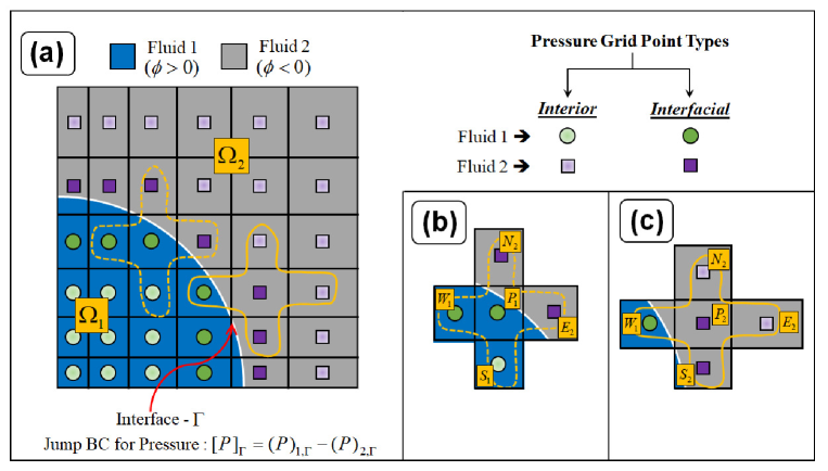
Figure 1: ($a$) A representative computational domain along with two-fluid interface and non-uniform grid distribution and of different types of pressure grid points for the two-fluid sub-domains ($\Omega_{1}$ and $\Omega_{2}$). Mixing of pressure grid point (from another fluid sub-domain) during the solution of pressure Poisson equation for interfacial pressure grid points is shown for $\Omega_{1}$ in ($b$) and for $\Omega_{2}$ in ($c$).

2.1 Single Fluid Formulation

For obtaining a single velocity and pressure field for both the fluids in a two-fluid flow, a single field formulation based governing equations and interfacial boundary conditions for SI-LSM are presented in a recent work from our research group; separately for two-phase flow without [9] and with [37] phase change. For two-phase flow without phase change considered here, the various functions used in a LSM and the formulation for sharp as well as diffuse interface LSM are presented in-detail by Shaikh et al. [9]; thus, the formulation is presented concisely in separate subsections below.

For the mathematical formulation, it is assumed that the interface is massless with zero-thickness, and no-slip in tangential velocity. Constant material properties are considered, but not equal for each phase, i.e., the bulk fluids are incompressible. The surface tension coefficient is assumed to be constant, and its tangential variation along the interface is neglected. The effects of radiation, viscous dissipation, and energy contribution due to interface stretching are neglected.

2.1.1 Governing Equations for Two-Fluid Flow Properties

Non-dimensional form of the conservation equations for the two-fluid flow (Navier-Stokes equations) are given as

Volume-Conservation (Continuity) Equation:

$$\nabla\cdot\mathbf{U}=0,$$ (1)

Momentum-Conservation Equation:

$$\frac{\partial\mathbf{U}}{\partial\tau}+\nabla\cdot\left(\mathbf{U}\mathbf{U}\right)=-\frac{\nabla P}{\chi_{i}}+\frac{1}{\chi_{i}Re}\nabla\cdot\left(2\eta_{i}\mathbf{D}\right)-\frac{1}{Fr^{2}}\hat{j},$$ (2)

where rate of deformation tensor, $\mathbf{D}=0.5\left[\nabla\mathbf{U}+\left(\nabla\mathbf{U}\right)^{T}\right]$. Furthermore, $\chi_{i}$ and $\eta_{i}$ are the non-dimensional density and viscosity; calculated using a sharp Heaviside function [9]. Also $\hat{j}$ is the unit vector for gravity ($\hat{j}=<0,-1>$). Using characteristic scales as $l_{c}$ for length and $u_{c}$ for velocity, the non-dimensional spatial as well as temporal coordinates, non-dimensional flow properties, and non-dimensional governing parameters (Reynolds number $Re$ and Froude number $Fr$), the non-dimensional variables in the above equations are defined as

$$\mathbf{X}=\frac{x}{l_{c}},\,\mathbf{U}=\frac{u}{u_{c}},\,\tau=\frac{tu_{c}}{l_{c}},\>P=\frac{p}{\rho_{1}u_{c}^{2}},\>Re=\frac{\rho_{1}u_{c}l_{c}}{\mu_{1}}\mbox{ and }Fr=\frac{u_{c}}{\sqrt{gl_{c}}}.$$

For the two-phase as compared to most of the single-phase flow, note that the above momentum equations consist of gravity force as the additional force while the force due to surface tension which also appears for a two-phase flow is incorporated in the SI-LSM as an interfacial boundary condition during the solution of pressure Poisson equation (obtained from the above volume conservation equation); presented below. Also note that the force due to surface tension is considered as a sharp surface force in the SI-LSM [9] while it is modeled as a volumetric force term (within the thickness of the diffused interface) in the above momentum equation for the DI-LSM [36].

2.1.2 Governing Equations for Two-Fluid Interface

Physically, the two-fluid interface is advected by the fluid-flow; obtained by solving the governing equations in the previous subsection. Mathematically, in a LSM, the unsteady interface advection is represented by an advection equation for a signed normal distance function representing the interface, i.e., level set function $\phi$. However, after the advection, the interface representing $\phi$ no more remains as a normal distance function and another equation called as reinitialization equations is solved using the pseudo transient approach. The reinitialization is essential for an accurate calculation of surface tension, jump terms, and thermophysical properties. Thus, the governing equations for the two-fluid interface are given as

Level-Set Advection (Mass-Conservation) Equation:

$$\frac{\partial\phi}{\partial\tau}+\mathbf{U}_{a}\cdot\nabla\phi=0,\thinspace\thinspace\thinspace\thinspace\thinspace\thinspace\thinspace$$ (3)

where $\mathbf{U}_{a}$ is the advection velocity which is equal to the bulk-velocity $\mathbf{U}$ (obtained from the solution of the above volume and momentum conservation equations). The above equation was derived from a mass conservation equation by Gada and Sharma [38].

Reinitialization Equation:

$$\frac{\partial\phi}{\partial\tau_{s}}+S\left(\phi_{o}\right)\widehat{n}\cdot\nabla\phi-S\left(\phi_{o}\right)=0,$$ (4)

where $S\left(\phi_{o}\right)$ is a sign function and $\tau_{s}$ is a pseudo time step. After getting the converged solution of Eq. (4), level set field will again become signed normal distance with respect to zero level set value. Here, partial differential equation based reinitialization (Sussman et al. [5]) is used.

2.1.3 Interfacial Boundary Conditions

In a computational fluid dynamics (CFD), the unsteady velocity field is obtained from the momentum conservation equation (Eq. (2)) and the pressure field is left with the volume conservation equation (Eq. (1)) which does not consist of any pressure term [1]; thus, a predictor-corrector method is used to convert the volume conservation equation into a pressure Poisson equation in a pressure projection method. While solving the pressure Poisson equation and the momentum equation for a two-phase flow in a single field formulation based SI-LSM, interfacial boundary conditions along with the boundary conditions for the flow properties at the boundary of the domain are required. The interfacial BCs involve jump boundary conditions for pressure and velocity at the interface $\Gamma$; given as

$$\left[P\right]_{\Gamma} = \frac{2}{Re}\left[\eta\right]\hat{N\centerdot}\left(\nabla U\centerdot\hat{N},\nabla V\centerdot\hat{N}\right)+\frac{\kappa}{We},$$ (5)

$${}[\mathbf{U}]_{\Gamma} = 0,$$

where the above equation for pressure is obtained by applying Newton’s II law of motion at the interface $\Gamma$ and a detailed derivation of the pressure-jump BC was presented by Shaikh et al. [9]. The interfacial force balance considers the force due to surface tension as the sharp surface-force which is balanced with both pressure force and normal viscous force in viscous flow across the interface [39].

The interfacial boundary condition across the interface is shown in Fig. 1. As shown in the figure, for pressure, the jump condition notation across the interface is expressed as ${\color[rgb]{0,0,0}{\color[rgb]{1,0,0}{\color[rgb]{0,0,0}[\cdot]_{\Gamma}=\left(\cdot\right)_{1,\Gamma}-\left(\cdot\right)_{2,\Gamma}}}}$; $\left(\cdot\right)_{1,\Gamma}$ and $\left(\cdot\right)_{2,\Gamma}$ are the value of the flow properties at the interface $\Gamma$ from the heavier and lighter phase in the $\Omega_{1}$ and $\Omega_{2}$ region, respectively.

3 Adaptive interface-Mesh un-Refinement

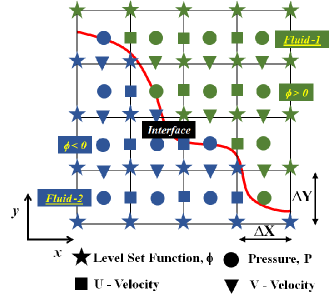
Figure 2: A representative 2D Cartesian grid along with the staggered grid points for flow-properties and level set function $\phi$ in a two-fluid problem.

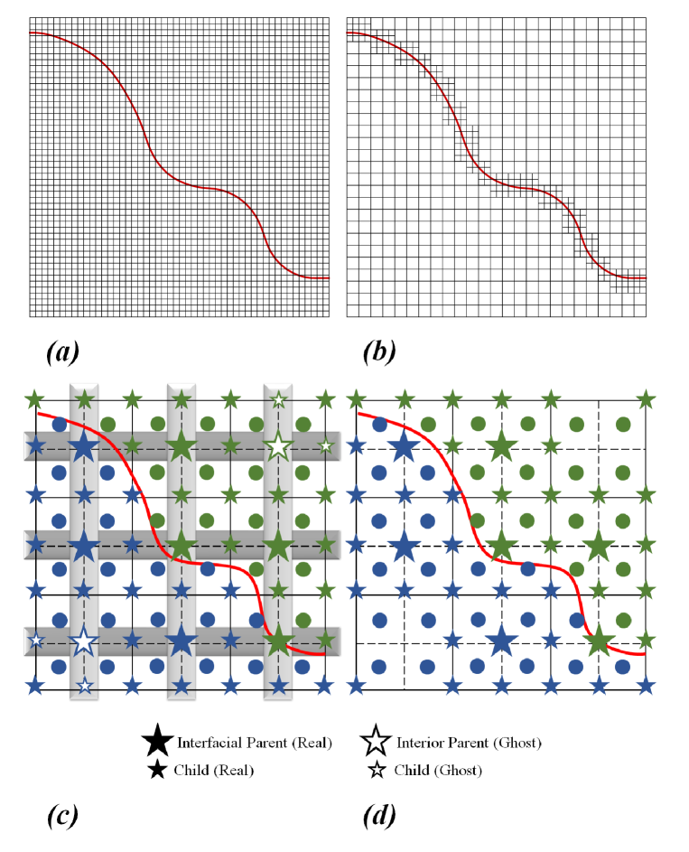
Figure 3: A representative Cartesian grid for a two-fluid system with an interface: ($a,c$) initial uniform grid at $\tau=0$ for the interface and at all time instants for the flow and ($b,d$) dynamically unrefined grid. Here, ($c$) and ($d$) show the various types of grid points considered to implement the instantaneous interface based dynamic mesh un-refinement. The unrefined interface grid in ($d$) is obtained from the uniform grid for the flow-properties in ($c$) after eliminating ghost-parent and ghost-child level set grid points. Note that a narrow band of the fine grid (at the interface) is shown in ($b$) for representative purpose only and a much wider band is used in the present method for accurate computations.

For the staggered grid used here, the grid points for pressure, velocity and level set function are shown in Fig. 2. For the implementation of the interface-mesh unrefinement, all level set grid points are tagged as a parent or a child grid point. All parent level set grid points are further tagged as interfacial or interior grid points. Finally, each parent and child grid point is tagged as real or ghost grid point. The various types of level set grid points are shown in Fig. 3. The figure also shows an interface representing the two-fluid. A representative 2D Cartesian grid is shown in Fig. 3($a$) as a uniform mesh for solving the Navier-Stokes equations (Eq. (1) and (2)) along with the interfacial boundary conditions (Eq. (5)); and Fig. 3($b$) as the adaptive unrefined interface mesh for solving the level set equations (Eq. (3) and (4)). The solution of the respective set of equations results in unsteady flow properties (U,V, and P) and level set function $\phi$. Fig. 3($b$) shows a merging of the four finer control volumes (CVs) in Fig. 3($a$) to a coarser control volume, for those CVs which are slightly away from the interface. This results in the unrefinement of the interface mesh which is away from the interface and the unrefinement is time-wise adaptive to the position of the interface which evolves with time $-$ called here as Adaptive interface-Mesh un-Refinement (AiMuR).

The implementation and algorithmic details for the adaptive unrefinement of the interface mesh (Fig. 3($b$)) $-$ from the fixed flow-properties mesh (Fig. 3($a$)) $-$ are presented with the help of Fig. 3($c$) and 3($d$). Fig. 3($c$) shows a tagging of each level set grid point as parent or child, interfacial or interior, and real or ghost grid points; and Fig. 3($d$) shows only real (not the ghost) grid points that lead to the AiMuR. The three types of tagging for each level set function grid point are as follows:

1. Tag as parent or child grid point: parent if both the running indices i and j are even; otherwise, child.

2. Tag parent grid points as interfacial or interior: all parent level set grid points with at least one adjoining neighbor (east/west/north/south) parent level set grid point in another fluid are tagged as an interfacial parent grid point. Identification of the interfacial and non-interfacial parent grid points are done by considering change in the sign of level set function $-$ interfacial parent grid point if the product of level set function at parent grid point $\phi_{P}$ and at any of the adjoining parent neighbor $\phi_{NB}$ is negative ($\phi_{P}\phi_{NB=W,E,S,N}<0$); otherwise, consider the grid point as interior parent grid point.

3. Tag as ghost or real: interior as ghost and interfacial as real, for the parent grid points; whereas, for the child grid points, the adjoining neighbor (north, south, east, and west) child grid points of a ghost interior parent grid point are considered as ghost and all the other child nodes in the domain are considered as real. Note that the common adjoining child neighbors of ghost interior parent grid points and real interfacial parent grid points are considered as real child grid points.

Based on the proposed definition of parent and child level set grid points and interface configuration shown in Fig. 3($c$), level set function grid points at the intersection of the horizontal strips and vertical strips (marked in the figure) are the parent level set grid points. Here, words real and ghost are used in the sense that level set equations are solved only for real grid points and not for ghost grid points. This classification of parent and child level set grid points into real and ghost grid points generates level set grid point distribution as finer in the interfacial region and coarser in the non-interfacial region. Implementing the tagging procedure (discussed above) for level set grid point distribution shown in Fig. 3($c$) and then eliminating the ghost parent and child nodes results in real grid points distribution as shown in Fig. 3($d$).

The above-discussed implementation results in a single level adaptive interface mesh unrefinement. However, the present unstructured adaptive grid-like distribution is implicitly achieved by the unrefinement using tagging and without involving any tree data structure. Once the unrefinement is done, the level set grid will have the same resolution as that of flow grid in the interfacial region while the level set grid away from interface will be coarser by the single-level. Limiting the refined grid close to the interface is justified since the value of the level set function $\phi$ close to the physically relevant interface $\phi=0$ is only numerically relevant $-$ $\phi$ values close to the interface are only involved in the calculation of interfacial parameters such as fluid properties, curvature, and jump in the flow properties.

Although the above implementation details for AiMuR are presented in Fig. 3 for one interfacial cell on each side of the interface, note that every interfacial parent level set grid point and its three neighbor parent level set grid points in all the four directions (east/west/north/south) are considered in the present work for a more accurate CMFD computations. Thus, the wider interfacial band is considered in the proposed AiMuR since the one interfacial cell-based AiMuR shown in Fig. 3($b$) leads to an inaccurate solution. Moreover, as commonly used in AMR [24, 32] and used here for a more efficient AiMuR, the adaption of the grid is done after certain number of time steps (instead of after every $\Delta\tau$); $50\Delta\tau$, $150\Delta\tau$, and $15\Delta\tau$ are considered for the dam break simulation, liquid jet breakup, and droplet coalescence problems (presented below), respectively. These time-periods of the unrefinment are obtained after an unrefinment time-period independence study, presented below in subsection 7.1. The periodic grid unrefinement justifies the need for the wider interfacial band of the finer grid. Further, it is ensured that the interface does not enter into unrefined region during the above mentioned time interval of the periodic unrefinement for the three problems considered in the present work.

4 Numerical Methodology

4.1 Solution of Volume and Momentum Conservation Equations

Numerical solution of volume and momentum conservation equations is obtained by the pressure projection method in the present study. Here, semi-implicit formulation is adopted wherein the volume conservation equation is treated implicitly and all the terms of the momentum conservation equation except advection term are treated implicitly. Temporal discretization of the corresponding equations (Eq. (1) and (2)) are given as

$$\nabla\cdot\mathbf{U}_{P}^{n+1}=0,$$ (6)

$$\frac{\mathbf{U}_{P}^{n+1}-\mathbf{U}_{P}^{n}}{\Delta\tau}+\nabla\cdot(\mathbf{U}_{P}^{n}\mathbf{U}_{P}^{n})=-\frac{\nabla P^{n+1}}{\chi_{i}^{n}}+\frac{1}{\chi_{i}^{n}Re}\nabla\cdot(2\eta_{i}^{n}\mathbf{D}^{n+1})-\frac{1}{Fr^{2}}\hat{j}.$$ (7)

4.1.1 Semi-Implicit Pressure Projection Method

In the pressure projection method, velocity field is predicted by neglecting the pressure term in Eq. (7); given as

$$\frac{\mathbf{U}_{P}^{*}-\mathbf{U}_{P}^{n}}{\Delta\tau}+\nabla\cdot(\mathbf{U}_{P}^{n}\mathbf{U}_{P}^{n})=\frac{1}{\chi_{i}^{n}Re}\nabla\cdot(2\eta_{i}^{n}\mathbf{D}^{*})-\frac{1}{Fr^{2}}\hat{j}.$$ (8)

Using the predicted velocity field $\mathbf{U^{*}}$, new time level pressure field is obtained by solving a pressure Poisson equation (obtained from Eq. (6) using a predictor-corrector method); given as

$$\nabla\cdot\left(\frac{\nabla P^{n+1}}{\chi_{i}^{n}}\right)=\frac{1}{\Delta\tau}\nabla\cdot\mathbf{U^{*}}.$$ (9)

Finally, by subtracting Eq. (8) from Eq. (7) and neglecting the velocity correction in the diffusion terms, continuity satisfying velocity field at the new time level is obtained as

$$\mathbf{U}_{P}^{n+1}=\mathbf{U}_{P}^{*}-\frac{\nabla P^{n+1}}{\chi_{i}^{n}}\Delta\tau.$$ (10)

While solving the pressure Poisson equation (Eq. (9)), an interfacial jump boundary condition for pressure is used; presented in the next subsection.

4.1.2 Implementation of Jump Boundary Condition for Pressure

In a two-fluid system, there will be a lower dimensional mass-less interface separating different fluids. As shown in Fig. 1($a$), for each fluid, there will be two types of control volumes: (1) interfacial and (2) interior. While solving pressure Poisson equation (Eq. (9)) for interfacial control volumes, as depicted by the computational stencil in Fig. 1($b$)-($c$), the resulting linear algebraic equation involves pressure from the other fluid that leads to a poor approximation of pressure gradient term across the interface. This was demonstrated by Liu et al. [40] using order-of-magnitude analysis.

The poor approximation is avoided by using a pressure jump as an interfacial boundary condition [40] while solving the pressure Poisson equation (Eq. (9)). The interfacial pressure boundary condition is obtained by incorporating force balance at the interface [9]; given as ${(p_{1}-p_{2})-\mathbf{((\hat{n}\cdot\sigma)_{1}-(\hat{n}\cdot\sigma)_{2})\cdot\hat{n}}=-\gamma\mathbf{\nabla\cdot\hat{n}}}$, here, $p$ is pressure, $\mathbf{\sigma}$ is viscous stress tensor, $\gamma$ is surface tension coefficient and $\mathbf{\hat{n}}$ is a normal unit vector; and subscripts 1 and 2 denote fluid-1 and fluid-2, respectively. This force balance at the interface takes care of the discontinuity in pressure across the two-fluid interface. Here, a finite volume method based generalized algebraic formulation of pressure Poisson equation (along with the interfacial jump boundary condition for pressure), proposed by Shaikh et al. [9], is used. The generalized formulation involves an additional source term for the interfacial control volumes that is zero for the interior control volumes for pressure.

4.1.3 Special Treatment for a Non-Uniform Grid

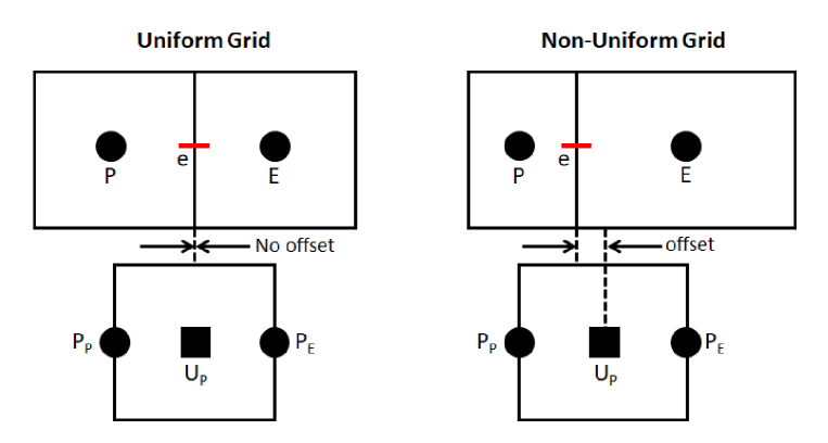
Figure 4: Offset between the centroid of velocity control volume and the face of pressure control volume.

Although Section 3 and Fig. 3 presents AiMuR on a uniform grid, the AiMuR and SI-LSM based in-house code is developed in the present work for both uniform and non-uniform Cartesian-grid. In this section, additional numerical details for non-uniform as compared to a uniform grid is presented. The essential difference in the numerical methodology is due to the staggered grid that results in a non-coinciding or an offset between the centroid of a velocity control volume and the associated face-center of the pressure control volume. This offset is shown in Fig. 4 for the east face of the non-uniform pressure control volume along with no such offset for the uniform grid.

The offset for the non-uniform grid results in a distance-based linear interpolations to compute the predicted velocities at the various face centers ($U_{e}^{*}$, $U_{w}^{*}$, $V_{n}^{*}$, and $V_{s}^{*}$) of the pressure control volume from the predicted velocities (Eq. (8)) at the centroid of the adjoining velocity control volumes ($U_{P}^{*}$, $U_{W}^{*}$, $V_{P}^{*}$, and $V_{S}^{*}$); thereafter, the $U_{e}^{*}$, $U_{w}^{*}$, $V_{n}^{*}$, and $V_{s}^{*}$ are used to calculate the predicted mass source on the right-hand side of the pressure Poisson equation (Eq. (9)). Furthermore, after obtaining the correct velocity field $\mathbf{U}_{P}^{n+1}$ from Eq. (10), the cell-center velocities are linearly interpolated to compute the velocity at the face-center of the pressure control volumes ($U_{e}^{n+1}$, $U_{w}^{n+1}$, $V_{n}^{n+1}$, and $V_{s}^{n+1}$). Finally, the face-center velocity are interpolated to obtain velocity at the corners of the pressure control volumes that is used to advect the level set function field.

4.2 Solution of Level Set Advection (Mass-Conservation) Equations

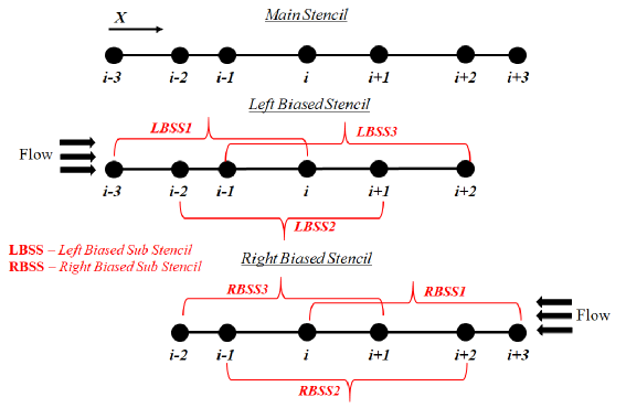
Figure 5: Stencil arrangement for $3^{rd}$ order accurate Essentially Non-Oscillatory (ENO) scheme for non-uniformly distributed grid points.

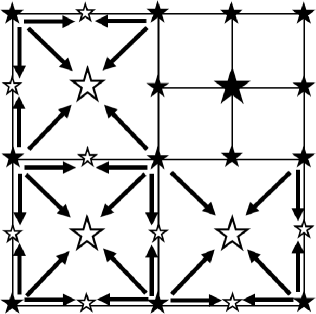
Figure 6: Interpolation of level set function at ghost grid point using real level set function grid points.

The numerical methodology for the solution of the Navier-Stokes equations (presented above) uses a physical law based finite volume method based algebraic formulation [1] while finite difference method is used for the discretization of the level set equations (Eq. (3) and (4)). Spatial (advection) term in the level set equations is discretized using a III-order accurate Essentially Non-Oscillatory (ENO) scheme (Jiang and Peng [41]). The temporal discretization of the level set advection equation is done using a III-order accurate Runge-Kutta scheme and using a I-order accurate forward difference for the reinitialization equation. Pseudo time step $\Delta\tau_{s}$ for the temporal term in the reinitialization equation is taken as 0.1 times of minimum grid size.

Although the formulation for the ENO scheme corresponding to a non-uniform grid is available for the finite volume method in literature [42], the formulation for finite difference method is presented here with the help of Fig. 5. The figure shows a non-uniform spacing based 7-point main-stencil, for implementing the ENO scheme on a non-uniform grid. The figure also shows that the main stencil is subdivided into two 6-point stencil: left and right biased stencils (LBS and RBS). These left/right stencils are further subdivided into three 4-point substencils: left substencil as LBSS1, LBSS2, and LBSS3; and right substencil as RBSS1, RBSS2, and RBSS3. Fitting a III-order Lagrange interpolation polynomial in each of these substencils results in a finite difference representation of the first derivative in the level set advection equation $-$ presented below for $\phi_{X}$ (representing ${\partial\phi}/{\partial X}$) at the various LBSS as

$$\phi_{X,i}^{LBSS1}=\phi_{i-3}\left(\frac{X_{i}^{2}-X_{i}X_{i-1}-X_{i}X_{i-2}+X_{i-1}X_{i-2}}{\left(X_{i-3}-X_{i}\right)\left(X_{i-3}-X_{i-2}\right)\left(X_{i-3}-X_{i-1}\right)}\right)\\ +\phi_{i-2}\left(\frac{X_{i}^{2}-X_{i}X_{i-1}-X_{i}X_{i-3}+X_{i-1}X_{i-3}}{\left(X_{i-2}-X_{i-3}\right)\left(X_{i-2}-X_{i-1}\right)\left(X_{i-2}-X_{i}\right)}\right)\\ +\phi_{i-1}\left(\frac{X_{i}^{2}-X_{i}X_{i-2}-X_{i}X_{i-3}+X_{i-2}X_{i-3}}{\left(X_{i-1}-X_{i-3}\right)\left(X_{i-1}-X_{i-2}\right)\left(X_{i-1}-X_{i}\right)}\right)\\ +\phi_{i}\left(\frac{1}{\left(X_{i}-X_{i-3}\right)}+\frac{1}{\left(X_{i}-X_{i-2}\right)}+\frac{1}{\left(X_{i}-X_{i-1}\right)}\right),$$ (11)

$$\phi_{X,i}^{LBSS2}=\phi_{i-2}\left(\frac{X_{i}^{2}-X_{i}X_{i-1}-X_{i}X_{i+1}+X_{i-1}X_{i+1}}{\left(X_{i-2}-X_{i-1}\right)\left(X_{i-2}-X_{i}\right)\left(X_{i-2}-X_{i+1}\right)}\right)\\ +\phi_{i-1}\left(\frac{X_{i}^{2}-X_{i}X_{i-2}-X_{i}X_{i+1}+X_{i-2}X_{i+1}}{\left(X_{i-1}-X_{i-2}\right)\left(X_{i-1}-X_{i}\right)\left(X_{i-1}-X_{i+1}\right)}\right)\\ +\phi_{i+1}\left(\frac{X_{i}^{2}-X_{i}X_{i-1}-X_{i}X_{i-2}+X_{i-1}X_{i-2}}{\left(X_{i+1}-X_{i}\right)\left(X_{i+1}-X_{i-2}\right)\left(X_{i+1}-X_{i-1}\right)}\right)\\ +\phi_{i}\left(\frac{1}{\left(X_{i}-X_{i-2}\right)}+\frac{1}{\left(X_{i}-X_{i-1}\right)}+\frac{1}{\left(X_{i}-X_{i+1}\right)}\right),$$ (12)

$$\phi_{X,i}^{LBSS3}=\phi_{i-1}\left(\frac{X_{i}^{2}-X_{i}X_{i+1}-X_{i}X_{i+2}+X_{i+1}X_{i+2}}{\left(X_{i-1}-X_{i}\right)\left(X_{i-1}-X_{i+1}\right)\left(X_{i-1}-X_{i+2}\right)}\right)\\ +\phi_{i+1}\left(\frac{X_{i}^{2}-X_{i}X_{i-1}-X_{i}X_{i+2}+X_{i-1}X_{i+2}}{\left(X_{i+1}-X_{i-1}\right)\left(X_{i+1}-X_{i}\right)\left(X_{i+1}-X_{i+2}\right)}\right)\\ +\phi_{i+2}\left(\frac{X_{i}^{2}-X_{i}X_{i-1}-X_{i}X_{i+1}+X_{i-1}X_{i+1}}{\left(X_{i+2}-X_{i}\right)\left(X_{i+2}-X_{i+1}\right)\left(X_{i+2}-X_{i-1}\right)}\right)\\ +\phi_{i}\left(\frac{1}{\left(X_{i}-X_{i-1}\right)}+\frac{1}{\left(X_{i}-X_{i+1}\right)}+\frac{1}{\left(X_{i}-X_{i+2}\right)}\right),$$ (13)

From the above values, the $\phi_{X,i}^{LBSS}$ is chosen as

$$\phi_{X,i}^{LBSS}=\begin{cases}\phi_{X,i}^{LBSS1}&\begin{array}[]{cc}if\end{array}\mid B\mid<\mid C\mid\&\mid A-B\mid<\mid B-C\mid\\ \phi_{X,i}^{LBSS3}&\begin{array}[]{cc}if\end{array}\mid B\mid>\mid C\mid\&\mid B-C\mid>\mid C-D\mid\\ \phi_{X,i}^{LBSS2}&\text{otherwise},\end{cases}$$ (14)

where

$$A=\frac{\phi_{i-3}-\phi_{i-2}}{X_{i-2}-X_{i-3}}+\frac{\phi_{i-1}-\phi_{i-2}}{X_{i-1}-X_{i-2}},\,\,\,\,B=\frac{\phi_{i-2}-\phi_{i-1}}{X_{i-1}-X_{i-2}}+\frac{\phi_{i}-\phi_{i-1}}{X_{i}-X_{i-1}}$$

$$C=\frac{\phi_{i-1}-\phi_{i}}{X_{i}-X_{i-1}}+\frac{\phi_{i+1}-\phi_{i}}{X_{i+1}-X_{i}},\,\,\text{and}\,\,D=\frac{\phi_{i}-\phi_{i+1}}{X_{i+1}-X_{i}}+\frac{\phi_{i+2}-\phi_{i+1}}{X_{i+2}-X_{i+1}}.$$

Similarly, the expression for $\phi_{X,i}^{RBSS}$ can be obtained and the ENO scheme based discretized form of $\phi_{X,i}$ in the level set advection equation (Eq. (3)) is given as

$$U\frac{\partial\phi}{\partial X}=\text{max}(U,0)\phi_{X,i}^{LBSS}+\text{min}(U,0)\phi_{X,i}^{RBSS}$$ (15)

For the AiMuR on a uniform or non-uniform Cartesian-grid, now the implementation details for the above ENO scheme are discussed. For the AiMuR, ghost grid points are considered in the stencil wherever needed while applying the ENO scheme for the real grid points; and are not needed for the interfacial boundary condition since we ensured a sufficiently wider band of the refined grid near the interface. This is done to ensure that the weights of neighboring $\phi^{\prime}$s in Eq. (11), (12) and (13) are computed only once (after the generation of uniform or non-uniform Cartesian-grid) and do not change with time $-$ they are not dynamic. Values of the level set function at the ghost grid points are computed by linear interpolation of the adjoining real grid points. This is shown in Fig. 6, where the arrows show the neighboring real child point values involved in the interpolation. In addition to the computation of ENO scheme, these interpolated level set function values at ghost grid points are utilized when ghost level set grid points turn into real level set grid points.

5 Solution Algorithm

1. Generate initial configuration of fluid-fluid interface for all the level set grid points. Initialize pressure and velocity as zero. Calculate the weights of ENO scheme based on the distribution of level set grid points.

2. Identify parent as well as child level set grid points (see section 3). Further, bifurcate them into real and ghost level set grid points.

3. Calculate the thermo-physical properties using a sharp Heaviside function [9]. Harmonic mean of the thermo-physical properties on the either side of the interface is considered for interfacial cells.

4. Calculate the advection and diffusion flux (in Eq. (8)) considering the continuity in velocity field and in its gradient at the fluid-fluid interface. Predict the velocity $\mathbf{U^{*}}$ at the new time level by solving Eq. (8). Here, III-order Lin-Lin total variation diminishing (TVD) [43] scheme is employed for discretizing the explicit advection term while the diffusion term is discretized using a central difference scheme.

5. Calculate the mass-source (RHS of Eq. (9)) by linearly interpolating predicted velocity $\mathbf{U^{*}}$ at the face-center of the pressure control volume.

6. Obtain the converged solution of the pressure Poisson equation (Eq. (9)) using the jump condition by Ghost Fluid Method (GFM).

7. Calculate the corrected velocity at the new time step (Eq. (10)). Linearly interpolate the corrected velocity at the face-center of the pressure control volume.

8. Obtain the level set advection velocity $\mathbf{U}_{a}$ at the real level set grid points using a linear interpolation of the velocity at the face-center of the pressure control volume. Advect the level set function field using Eq. (3) for real level set grid points using the methodology explained in subsection 4.2.

9. Interpolate the advected level set function field at ghost level set grid points from the real level set grid points (see Fig. 6).

10. Set the level set field as normal signed distance function by solving level set reinitialization equation (Eq. 4) for real level set grid points.

11. Repeat step 9.

12. Go to step 2 until the stopping criterion is met.

6 Validation and Qualitative Performance Study of AiMuR based SI-LSM

Table 2: Grid size for the five different grid types: uniform coarse grid ($U_{c}$), non-uniform coarse grid ($NU_{c}$), non-uniform coarse grid with AiMuR ($NU_{c}^{AiMuR}$), uniform fine grid with AiMuR ($U_{f}^{AiMuR}$) and uniform fine grid ($U_{f}$) corresponding to the dam break, jet breakup and droplet coalescence problem .

	DB	JB	DC
$U_{c}$, $NU_{c}$, and $NU_{c}^{AiMuR}$	100$\times$50	35$\times$200	100$\times$200
$U_{f}$ and $U_{f}^{AiMuR}$	144$\times$80	50$\times$300	200$\times$400

In order to present the validation of the proposed numerical methodology and performance study, three different types of two-phase flow problems are considered: Dam-Break (DB), Jet-Breakup (JB) and Drop-Coalescence (DC). The dominant force is gravity, inertia and capillary force in the DB, JB and DC simulations, respectively. The DB simulation does not involve breakup of interface while the JB and DC problems involve more rigorous interface dynamics with break-up of interface that leads to a droplet formation. Computational setup corresponding to the three problems are shown in Fig. 7. A performance study of the proposed AiMuR based SI-LSM is presented here by considering the adaptive unrefinement of the interface mesh on both uniform and non-uniform grid. However, since the result on a non-uniform as compared to the uniform grid is more accurate, the AiMuR on a non-uniform grid is considered on a coarser grid while the AiMuR on a uniform grid is presented on a finer grid; the respective AiMuR based SI-LSM is represented here as $NU_{c}^{AiMuR}$ and $U_{f}^{AiMuR}$. Considering our in-house codes for the novel AiMuR based SI-LSM as well as the traditional SI-LSM, the scope of the present performance study is to compare the relative accuracy of the novel and traditional SI-LSMs (on uniform and non-uniform grid), with the accuracy obtained by comparing with the published experimental and numerical results for the DB, JB and DC problems. The relative accuracy is presented qualitatively in this section and and quantitatively in the next section. The resulting five different grid types of SI-LSM are presented in Table 2 along with the associated grid size considered in the present simulations. Note that grid size mentioned in Table 2 for $NU_{c}^{AiMuR}$ and $U_{f}^{AiMuR}$ is without performing unrefinement for the level set function.

For the five grid types ($U_{c}$, $NU_{c}$, $NU_{c}^{AiMuR}$, $U_{f}^{AiMuR}$, and $U_{f}$), the grid resolution of uniform coarse grid $U_{c}$ (Table 2) is intentionally chosen such that, numerical result will not be accurate enough while the finer grid size $U_{f}$ is kept fine enough to produce reliable numerical results. Furthermore, non-uniform coarse grid ($NU_{c}$) is chosen such that it comprises of same number of control volumes as that of uniform coarse grid ($U_{c}$). However, grid stretching in $NU_{c}$ is done such that the grid resolution in interfacial region is comparable to uniform fine grid ($U_{f}$). For grid case $NU_{c}^{AiMuR}$, control volume distribution for pressure and velocity is same as that for $NU_{c}$. Nevertheless, mesh unrefinement strategy is incorporated in $NU_{c}^{AiMuR}$, which creates level set resolution equivalent to $NU_{c}$ in interfacial region and coarser resolution in non-interfacial region. Similar discussion is also applicable for grid types $U_{f}$ and $U_{f}^{AiMuR}$. Similar to $NU_{c}$, both $NU_{c}^{AiMuR}$ and $U_{f}^{AiMuR}$ possess grid resolution equivalent to that of $U_{f}$ near the interface.

Based on the characteristic of the grid types selected in present work, one can predict that computational time for $U_{f}$ will be maximum among all, which will get reduced after applying mesh unrefinement ($U_{f}^{AiMuR}$). Computational time associated with $U_{c}$ and $NU_{c}$ should be nearly same, as they have same number of control volumes. However, it largely depends on the trend of iterations while solving pressure Poisson equation and also up to some extent on additional computational operations required for $NU_{c}$ as compared to $U_{c}$. Computational time for $NU_{c}^{AiMuR}$ should be less than that required by $NU_{c}$. Difference in computational time for $NU_{c}^{AiMuR}$ ($U_{f}^{AiMuR}$) and $NU_{c}$ ($U_{f}$) will depend on the number of unrefined level set grid points (which implicitly depends on how the interface evolves with time) in $NU_{c}^{AiMuR}$ ($U_{f}^{AiMuR}$). The hypothesised computational time for the various grid types are compared quantitatively in the next section.

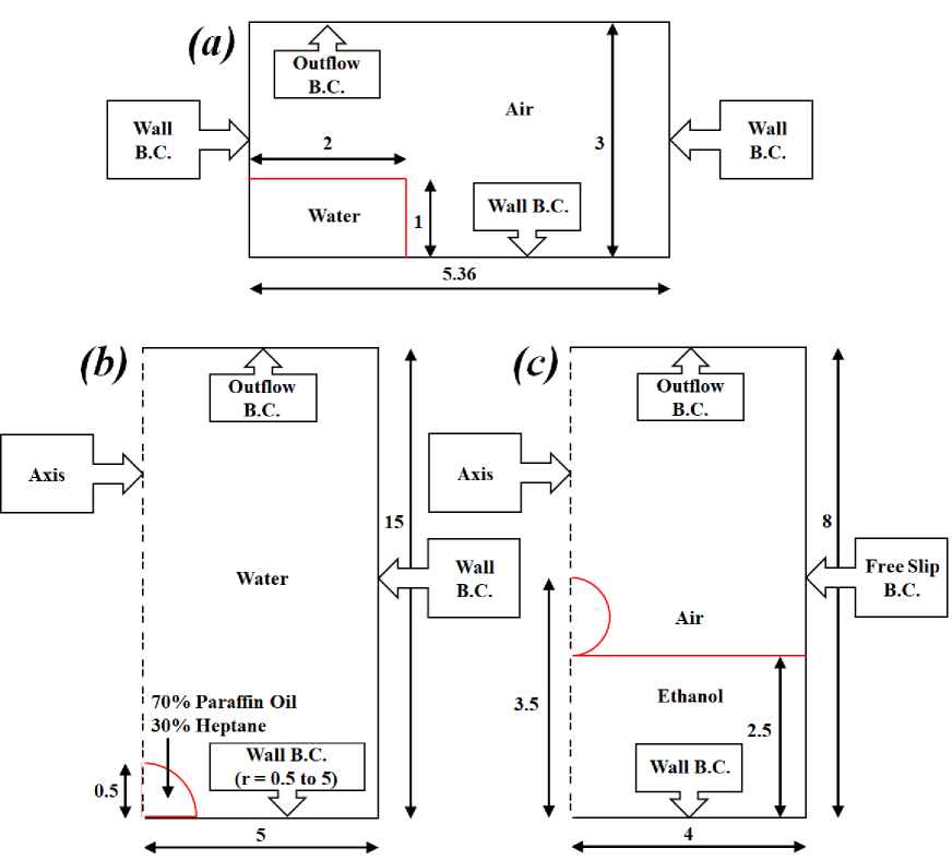
Figure 7: Computational setup for (a) Dam break simulation (b) Breakup of a liquid jet and (c) Coalescence of a stagnant ethanol drop at air-ethanol interface.

6.1 Dam Break Simulation

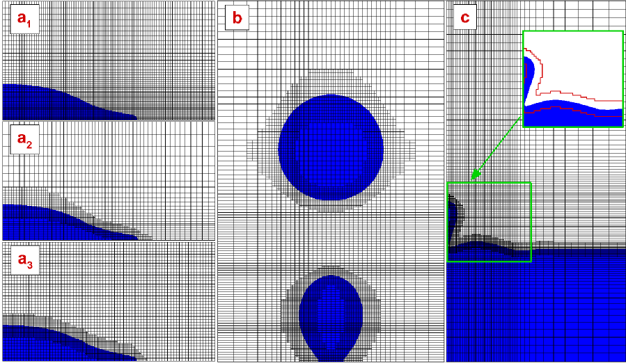
Figure 8: Interface (level set) mesh for ($a$) dam break simulation, ($b$) liquid jet-breakup, and ($c$) drop coalescence problems. The interface mesh shown in $(a_{1})$, $(a_{2},b,c)$, and $(a_{3})$ is for $NU_{c}$, $NU_{c}^{AiMuR}$, and $U_{f}^{AiMuR}$, respectively. The adaptive unrefined instantaneous interface mesh is at $\tau=1.5$ for ($a_{2}$) and ($a_{3}$), $\tau=150$ for ($b$), and $\tau=0.55$ for ($c$).

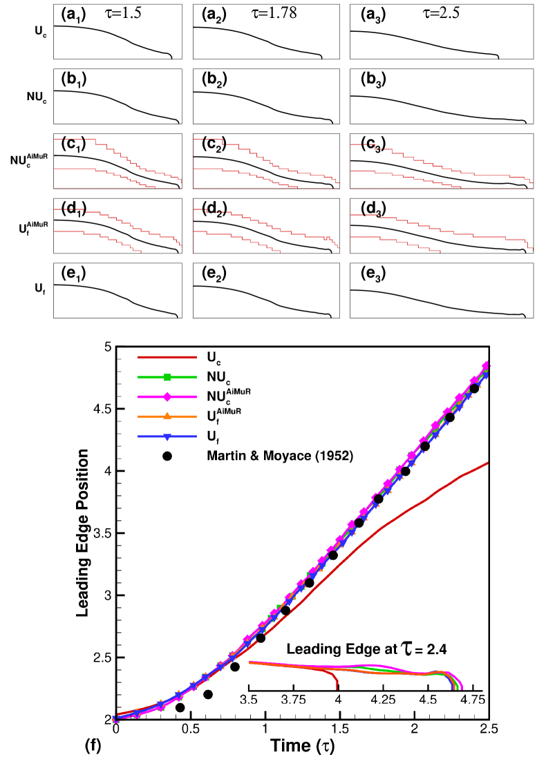
Figure 9: Dam break simulation at $Re=3\times 10^{6}$ and $Fr=1$. For the present SI-LSM on the various grid types (Table 2), ($a-e$) instantaneous interface position at three different time instances and ($f$) comparison of the present numerical and the published experimental [44] result. The stair-stepped lines for $NU_{c}^{AiMuR}$ and $U_{f}^{AiMuR}$ represent the interfacial region (in between the lines) outside which the level set grid points are dynamically unrefined.

Computational setup for this problem in Fig. 7($a$) shows a water column that is allowed to collapse under the effect of gravity. For the non-uniform Cartesian grid generation, a grid transformation function [45] is used that is given as

$$X/Y=L\lambda\left(1+\frac{\text{sinh}\left(\beta\left(\xi-A\right)\right)}{\text{sinh}\left(\beta A\right)}\right),$$ (16)

where,

$$A=\frac{\text{ln}\left(\frac{1+\lambda\left(e^{\beta}-1\right)}{1+\lambda\left(e^{-\beta}-1\right)}\right)}{2\beta}.$$

The value of different tuning parameters for non-uniform distribution in X and Y directions are $\beta_{X}=2.5$, $\beta_{Y}=3.1$, $\lambda_{X}=0.466$, and $\lambda_{Y}=0.066$. Resulting non-uniform grid distribution is shown in Fig. 8($a_{1}$) for $NU_{c}$ and Fig. 8($a_{2}$) for $NU_{c}^{AiMuR}$; and Fig. 8($a_{3}$) shows adaptive unrefined uniform grid $U_{f}^{AiMuR}$. Note that the adaptive unrefined grid in Fig. 8($a_{2},a_{3}$) corresponds to $\tau=1.5$. For instantaneous interface position, Fig. 9($a$)-($e$) shows excellent agreement between the present results on the various types of SI-LSM on uniform/non-uniform grids (with or without interface mesh unrefinement) except the present result on $U_{c}$. This is also demonstrated for the leading edge distance in Fig. 9($f$) by comparing with a benchmark experimental results [44].

6.2 Breakup of a Liquid Jet

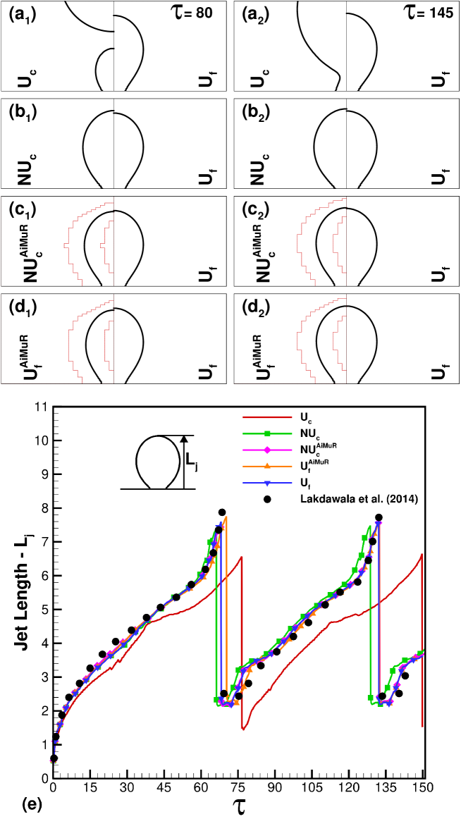
Figure 10: For jet breakup study at $Re=396$, $We=1.27$, and $Fr=5.44$, comparison of instantaneous interface obtained from $U_{c}$, $NU_{c}$, $NU_{c}^{AiMuR}$, and $U_{f}^{AiMuR}$ (left) with that obtained from $U_{f}$ (right) after $(a_{1}-d_{1})$ first jet breakup and $(a_{2}-d_{2})$ second jet breakup at time instances $\tau=80$ and $145$, respectively. Temporal variation of jet length $L_{j}$ obtained in the present work is plotted in ($e$) and compared with the published numerical results [46].

Computational setup for this problem is shown in Fig. 7($b$), where a lighter liquid is injected (against the gravity) in the heavier liquid with a constant velocity $0.15$ m/s. For the present problem, as long as the surface tension force dominates over the buoyancy force, the jet will keep on rising. Once buoyancy force exceeds the surface tension force, a neck forms and a droplet gets detached from the jet. The detached droplet continues to rise in the heavier stagnant fluid and the jet will regain its original shape.

Number of control volumes employed for the present jet breakup problem is presented in Table 2. For $NU_{c}$ and $NU_{c}^{AiMuR}$, gird clustering is implemented in both radial and axial direction, that results in almost same grid resolution to that for the fine uniform grid ($U_{f}$) in the breakup region. Distribution of level set function grid points after performing unrefinement on a non-uniform grid is shown in Fig. 8($b$) at a time instance $\tau=150$. Results for the interface dynamics corresponding to breakup of two droplets from the inlet jet are shown in Fig. 10. The instantaneous interface at $\tau=80$ and $\tau=145$ in Fig. 10($a$)$-$($d$) shows an excellent agreement between the present results on a coarse non-uniform grid (with and without unrefinement) as compared to the uniform grid. Similar agreement between the results on the various grid types and also with the results reported in Lakdawala et al. [46] is shown in Fig. 10($e$), for the temporal variation of jet length $L_{j}$; except for the result on uniform coarse grid $U_{c}$, which experiences late breakup of the jet as the interplay between surface tension and buoyancy force is not captured well because of insufficient grid cells in radial and axial direction.

6.3 Coalescence of an Ethanol Droplet

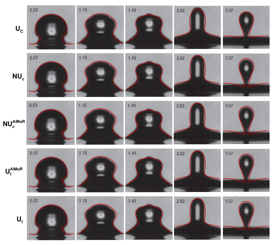
Figure 11: For coalescence study of an ethanol droplet (of diameter $1.07$ mm) in air, comparison of the temporal variation of present SI-LSM based numerically obtained instantaneous interface on five different grid types (Table 2) with experimental results of Blanchette and Bigioni [47]. The time instant marked above (0.53, 1.15, 1.40, 2.62 and 3.57) are in milli-second and the present numerically obtained interface is shown as line contour.

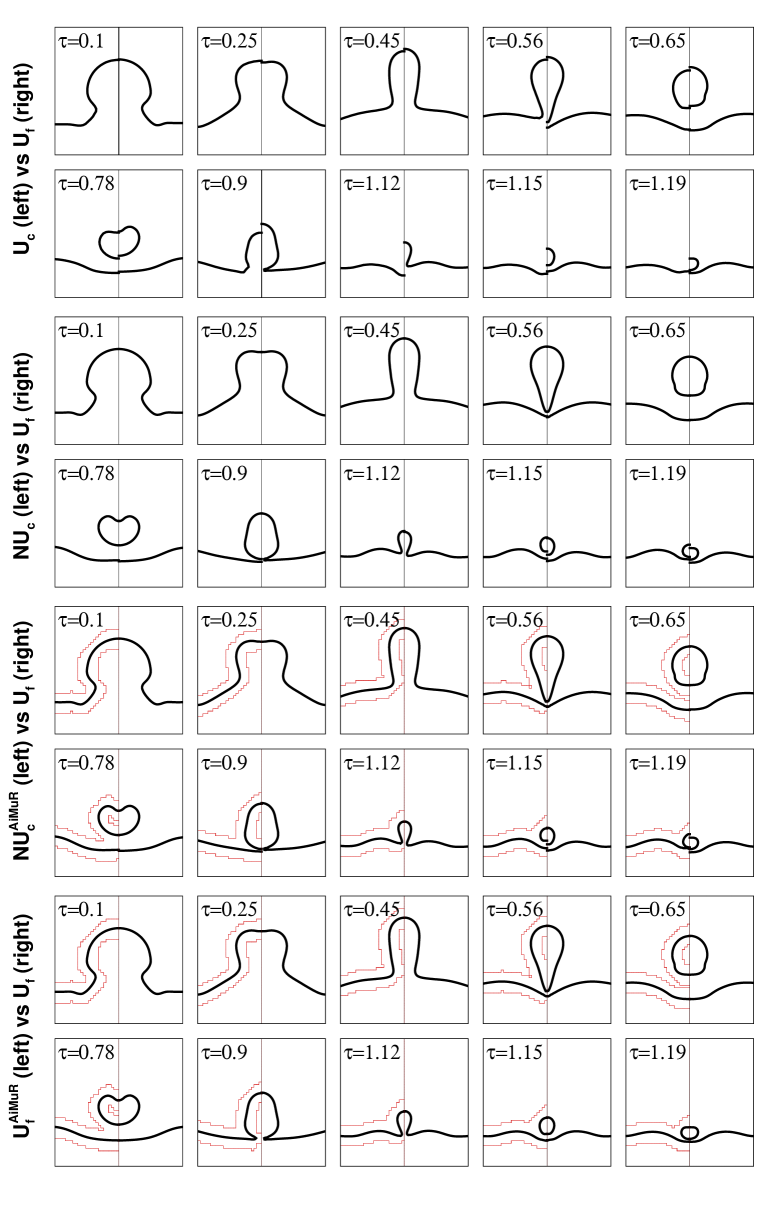
Figure 12: For coalescence dynamics of an ethanol droplet in air, comparison of temporal variation of instantaneous interface obtained for $U_{c}$, $NU_{c}$, $NU_{c}^{AiMuR}$, and $U_{f}^{AiMuR}$ (left) with that obtained for $U_{f}$ (right).

Computational set-up for the coalescence dynamics of an ethanol droplet of diameter $1.07$ mm, surrounded by air, over a pool of ethanol is shown in Fig. 7($c$)); and the unrefined non-uniform interface-mesh at $\tau=0.55$ is shown in Fig. 8($c$). Fig. 11 shows an excellent agreement between the instantaneous interface obtained on the various grid types and the experimental results reported by Blanchette and Bigioni [47]. However, at time instance $3.57$ ms, the present result for $U_{c}$ as compared to the result on other grid types shows a much thicker neck that indicates a delay in the pinch-off and the resulting formation of secondary droplet.

As compared to the time-duration just before the first pinch-off, Fig. 12 shows the temporal variation of the instantaneous interface for a longer time-duration corresponding to the second pinch-off of the secondary droplet. The figure shows that our result for the non-uniform grid with or without unrefinement agrees very well with the result on the finer uniform grid. However, the present result on a coarser uniform grid shows a slight delay in the first pinch-off of the primary droplet and thereafter it does not show the second pinch-off that is seen in the present results on the other grid types.

7 Unrefinement Time-Period Independence and Order-of-Accuracy Studies

7.1 Unrefinement Time-Period Independence Study

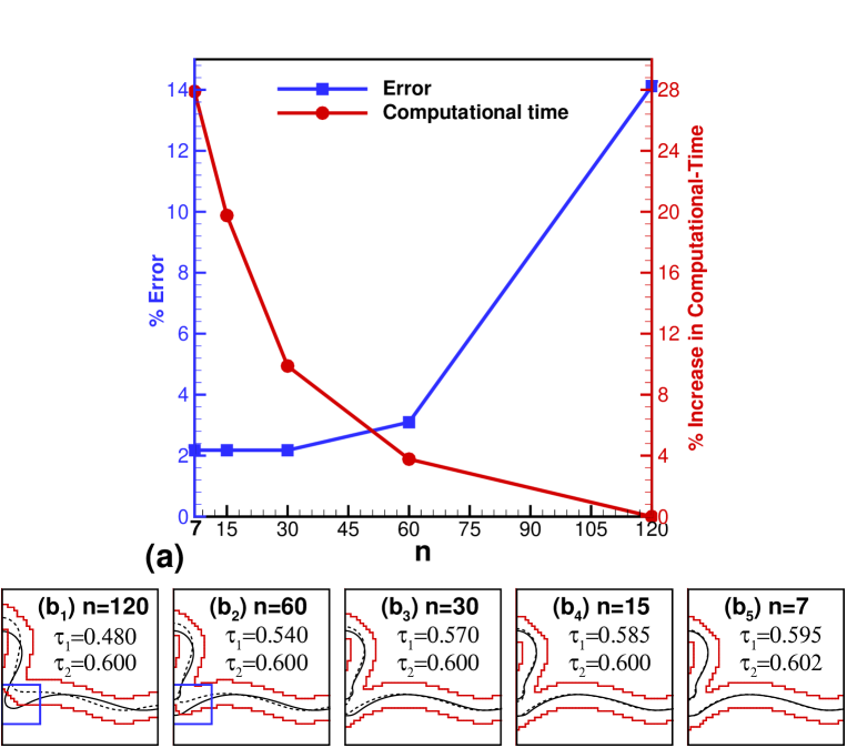
Figure 13: For the droplet coalescence problem, unrefinement time-period independence study of the present AiMuR on a uniform $200\times 400$ grid: ($a$) variation of % error and % increase in computational-time with decreasing number ($n$) of the time-step $\Delta t$ after which the interface-mesh is periodically-unrefined; and ($b_{1}$)-($b_{5}$) instantaneous interface obtained for the different values of $n$. The % error is for the first pinch-off time reported by Blanchette and Bigioni [47]. For ($b_{1}$)-($b_{5}$), the region in-between the red-curves corresponds to the fine-mesh region, with unrefined coarser-mesh outside this region; and the dashed and solid black-lines represent the interface at a time-instant corresponding to the beginning ($\tau_{1}$) and end ($\tau_{2}$) of the associated unrefinement time-period, respectively.

For the present AiMuR, the periodic unrefinement of the interface mesh is done after certain number $n$ of the time-step $\Delta t$ that results in the time-period for the unrefinement as $n\Delta t$ . Thus $n$ is a numerical parameter for the present method that is problem dependent and determined here from an unrefinement time-period independence study; similar to the grid-independence and time-step independence studies commonly used in CFD. The time-period independence study is presented in Fig. 13($a$), for the uniform grid based AiMuR and the droplet-coalascence problem. The figure shows an asymtotic decrease in the error with increasing $n$, with almost no change in the error after $n=15$. Thus, $n=15$, i.e., the periodic-unrefinement after every $15^{th}$ time-step, is chosen for the AiMuR based simulation of the coalascence of an ethanol droplet in air. The figure also shows an almost $20\%$ increase in the computational time as $n$ decreases from $120$ to $15$.

The unrefinement after certain number of time-steps, instead of after every time-step, is due to the fact that the present AiMuR involves a wider band of finer mesh near the interface. The fine-mesh region, along with the interface extreme positions, during the time-interval of the unrefinement is shown in Fig. 13($b_{1}$)-($b_{5}$) for various values of $n$. For the cases with $n=120$ and $60$, the figure shows that the interface moves outside the fine-mesh region during the time period $n\Delta t$ of the unrefinement; thus resulting in the larger error as seen in Fig. 13($a$). The unrefinement time-period independence study ensures that the fluid-fluid interface stays within the fine-mesh region for an accurate solution. Similar unrefinement independence study for the other problems resulted in $n=50$ for the dam break problem and $n=150$ for the liquid jet breakup problem.

7.2 Order of Accuracy Study

For a multiphase flow solver, order of accuracy study is widely reported for a problem on decaying oscillations of a capillary wave that has an analytical solution (Prosperetti [48]). Thus, after ensuring the verification of our numerical with the analytical solution, Fig. 14($a$) presents an order of accuracy study for this problem. The computational setup for this problem can be found in Gerlach et al. [49]; error is defined as $L_{2}$ norm of the difference between time-wise variation of the non-dimensional relative amplitude computed numerically and that obtained analytically. The figure shows that the order of accuracy of our SI-LSM on a uniform grid, with and without AiMuR, is between first and second order; almost same as that seen in the figure for the refined level-set grid method of Hermann [35]. For a comparative study, the figure also presents the order of accuracy study of seven other numerical methods: front-tracking method [50], Gerris flow-solver [24] (volume-of-fluid implementation with generalised height-function curvature calculation for quadtree and octree discretizations), PROST [51] (volume-of-fluid implementation with a parabolic reconstruction of surface tension) and CLSVOF [52] (coupled level-set volume-of-fluid formulation) implementations of Gerlach et al.[49], CSF-VOF [53] (continuous surface force method based modelling of surface tension in volume-of-fluid framework), and VOF-NIFPA-1 [54] (VOF implementation with non-intersecting flux polyhedron advection (NIFPA) scheme for the advection of volume fraction) and Conservative DI [55] (diffuse-interface) implementations of Mirjalili et al. [56] . The figure shows that the Gerris, PROST, and CLSVOF are almost second order accurate while the other six multiphase flow solvers (including our SI-LSM) exhibit an order of accuracy between first and second order. It is worth noting from the figure that the present SI-LSM as compared to the other numerical methods is most accurate for the coarser grid resolution of $N=8$ Whereas, on relatively finer grid resolution of $N=64$, it can be seen that our SI-LSM is more accuracte than the front-tracking, CSF-VOF, conservative DI and RLSG.

Order of accuracy study is also presented in Fig. 14($b$) for the same dam-break simulation (Fig. 7($a$)),considering the mass-error since this is the biggest disadvantage of the level set method [6]. With grid refinement, the convergence of the mass-error (at some particular time-instant) in the figure shows that the present present AiMuR based LSM is somewhere between first and second order accurate; same as concluded from Fig. 14($a$). Using the physical interpretation of Heaviside function, proposed [38] and later used in the previous work from our reasearch group [36, 57], the mass error is computed here as

$$\text{\% Mass Error}=100\times\frac{1}{\tau_{max}}\int_{0}^{\tau_{max}}\frac{\left|\sum_{i,j}H_{i,j}^{\tau}\Delta V_{i,j}-\sum_{i,j}H_{i,j}^{o}\Delta V_{i,j}\right|}{\sum_{i,j}H_{i,j}^{o}\Delta V_{i,j}}d\tau,$$ (17)

where, $H_{i,j}^{o}$ is the initial Heaviside function and $H_{i,j}^{\tau}$ is Heaviside function at a particular time instance $\tau$.

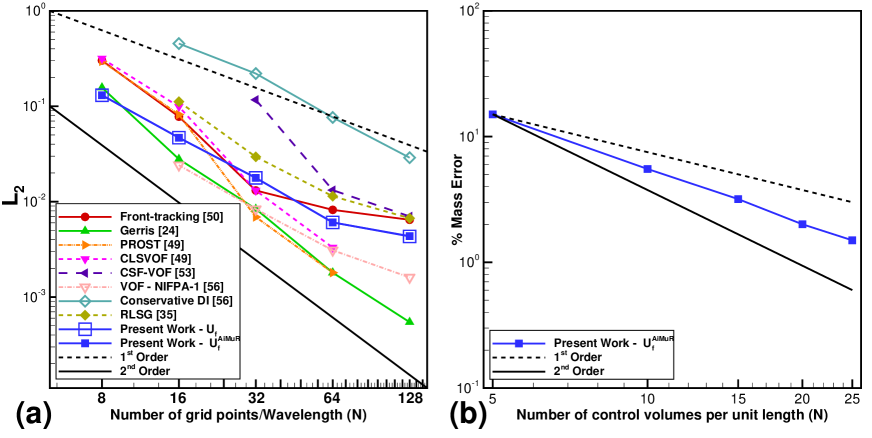
Figure 14: With increasing grid refinement levels, variation of ($a$) $L_{2}$ norm of the error (between the present/published mumtiphase solvers and analytical solution [48]) for the time-wise variation of the non-dimensional relative amplitude of a damped capillary wave (for $\rho_{1}=\rho_{2}=1$, $\mu_{1}=\mu_{2}=0.064720863$, and Ohnesorge number $Oh=1/\sqrt{3000}$) and (b) mass-error for the $U_{f}^{AiMuR}$ based dam-break simulation.

8 Quantitative Performance Study

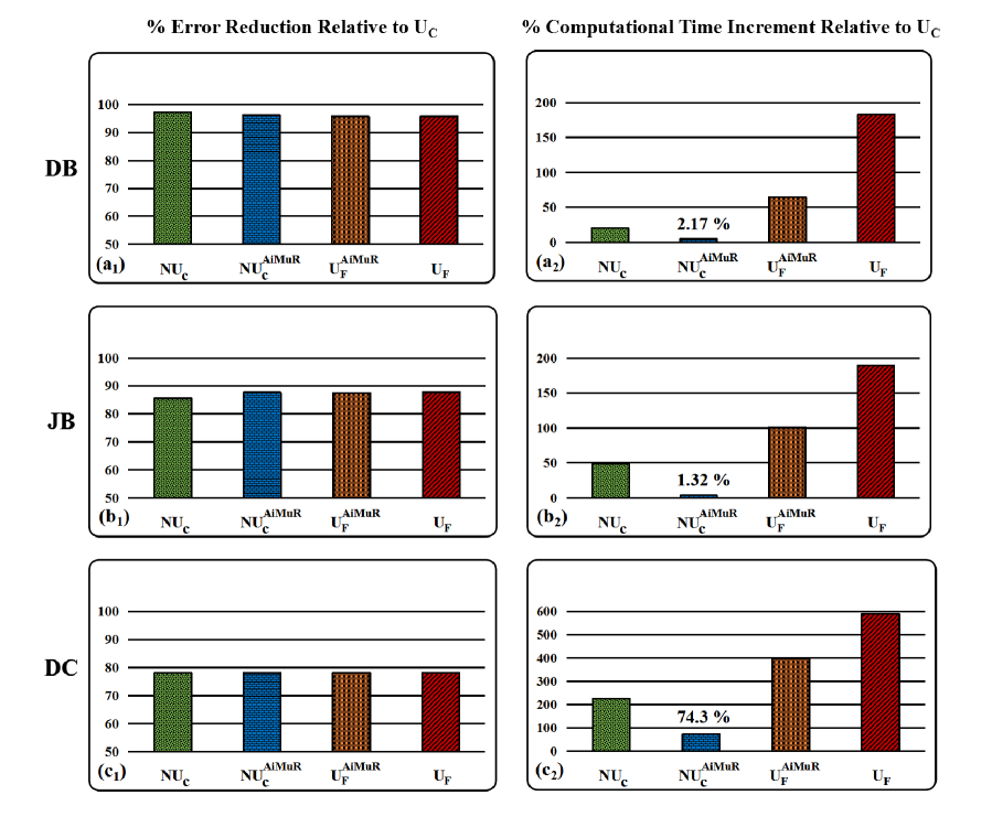
Figure 15: Variation of the performance parameters (Eq. (18)) for the present novel SI-LSM and traditional SI-LSM on the various grid types (Table 2) for $(a)$ dam break, $(b)$ jet breakup, and $(c)$ drop coalescence problems.

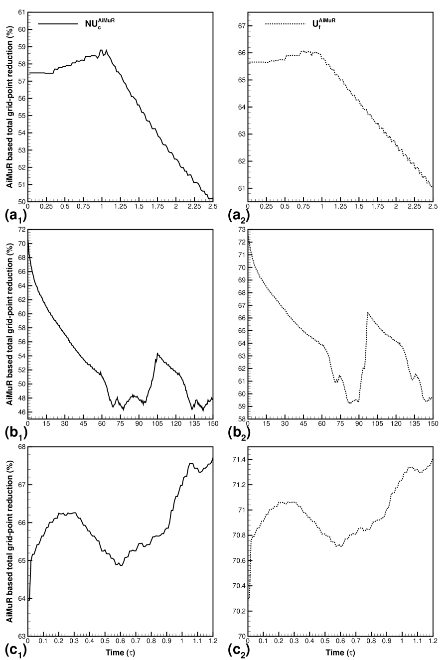
Figure 16: Temporal variation of AiMuR based total grid-point reduction (%) for the level set function on the $(a_{1},b_{1},c_{1})$ non-uniform coarse grid $NU_{c}$ and $(a_{2},b_{2},c_{2})$ uniform fine grid $U_{f}$, for $(a_{1},a_{2})$ dam break, $(b_{1},b_{2})$ jet breakup and $(c_{1},c_{2})$ droplet coalescence problems.

For the three different two-phase problems, the above comparison of the unsteady interface dynamics on the various grid types and also with the published numerical/experimental results clearly demonstrates the superiority of the SI-LSM on the non-uniform grid and unrefinement as compared to that on the uniform grid. Almost similar superiority of the $NU_{c}$, $NU_{c}^{AiMuR}$, and $U_{f}^{AiMuR}$ as compared to $U_{c}$ was demonstrated qualitatively above and presented quantitatively here.

The quantitative representation of the relative performance considers the total computational time (including the time required for the interpolation and the inter-grid transfer) along with the computational accuracy to distinguish the relatively superior performance of $NU_{c}$, $NU_{c}^{AiMuR}$, and $U_{f}^{AiMuR}$ as compared to $U_{c}$. Thus, for a quantitative representation, a detailed performance study is carried out by defining two performance parameters: % Error Reduction and % Computational Time Increment; given as [36, 57, 58, 37]

$$\%\,\,\text{Error}\,\,\text{Reduction}=\left(1-\frac{\text{Error}_{grid-type}}{\text{Error}_{U_{C}}}\right)\times 100,$$

$$\%\,\,\text{Computational}\,\,\text{Time}\,(C.T.)\,\,\text{Increment}=\left(\frac{C.T.{}_{grid-type}}{C.T.{}_{U_{C}}}-1\right)\times 100,$$ (18)

where a grid-type corresponds to $NU_{c}$, $NU_{c}^{AiMuR}$, $U_{f}^{AiMuR}$, and $U_{f}$. Further, present performance study is carried out using coarse uniform grid ($U_{c}$) as a reference grid for all the problems. In order to calculate the error associated with the present numerical results on various grid types, as compared to the published experimental/numerical results, certain parameter is selected in each problem. The parameter considered for calculating the error of the present SI-LSM corresponds to leading edge distance reported by Martin and Moyce [44] at time $\tau=2.4$, jet breakup length reported by Lakdawala et al. [46] (after second breakup) at time $\tau=145$, and first pinch-off time reported by Blanchette and Bigioni [47] for Dam-Break (DB), Jet-Breakup (JB) and Drop-Coalescence (DC) problems, respectively.

For the three sufficiently different two phase flow problems, the performance parameters (Eq. (18)) for the present novel and traditional SI-LSM on various grid types are shown in Fig. 15. As discussed in previous subsection, the error reduction in Fig. 15 demonstrates a quantitative (in terms of accuracy) evidence of almost same superiority of the $NU_{c}$, $NU_{c}^{AiMuR}$, and $U_{f}^{AiMuR}$ as compared to $U_{c}$. Whereas, the computational time increment clearly demonstrates the relative superiority of the $NU_{c}$, $NU_{c}^{AiMuR}$, and $U_{f}^{AiMuR}$, with the least computational time increment by the SI-LSM on $NU_{c}^{AiMuR}$ as compared to that on $NU_{c}$ and $U_{f}^{AiMuR}$. Theoretically, computational time for grid type $NU_{c}$ should be same as that for $U_{c}$ (as both of them are having same number of control volumes). Nevertheless, since $NU_{c}$ as compared to $U_{c}$ requires more iterations for solving pressure Poisson equation, $NU_{c}$ results in more computational time. Application of AiMuR on $NU_{c}$ reduces this overhead in computational time. This is seen in Fig. 15($a_{2},b_{2},$), with a negligible increase in computational time by $NU_{c}^{AiMuR}$ as compared to $U_{c}$. Further, the figure also shows that computational time demanded by $U_{f}$ gets reduced after applying the mesh unrefinement.

After applying AiMuR strategy on either uniform or non-uniform grid, the reduction in computational time is correlated with AiMuR based total grid-point reduction (%) that is shown in Fig. 16. The figure shows that instantaneous value of AiMuR based total grid-point reduction (%) for level set function is more than 45% for the problems studied here. Time-wise increase or decrease of AiMuR based total grid-point reduction (%) in Fig. 16 also implicitly represents the dynamics of fluid-fluid interface, i.e., spreading of the fluid-fluid interface in computational domain and AiMuR based total grid-point reduction (%) are inversely related. In dam break problem, gradual decrease in AiMuR based total grid-point reduction (%) is due to the interface spreading after the collapse of the water column. Similarly, in jet breakup, initial decrement in total grid-point reduction (%) is because of the continuous injection of fluid. After the first breakup, an increase in total grid-point reduction (%) is attained as soon as the detached droplet escapes the computational domain, followed by another decrease-increase cycle. For drop coalescence problem, an increase in AiMuR based total grid-point reduction (%) after first pinch off corresponds to the smaller daughter droplet size. Among all grid combinations, $NU_{c}^{AiMuR}$ is found to be computationally most efficient since it produces numerical results of almost same accuracy as that on a fine uniform grid ($U_{f}$) and requires a computational time almost same as that on coarse uniform grid ($U_{c}$).

Concluding Remarks

In the present work, numerical methodology for simulating multi-phase flows on dynamically unrefined uniform as well as non-uniform level set mesh is proposed, where unrefinement is carried out away from the interface location. The dynamic unrefinement is done for the Cartesian interface mesh corresponding to level set function only. Consequently, higher order schemes based solution of level set equations (advection and reinitialization) is obtained on almost half of the grid in the region away from the interface. Further, ENO scheme with varying weights is used to solve mass conservation equation on highly stretched non-uniform grids. To demonstrate the numerical accuracy and computational efficiency of the proposed AiMuR based SI-LSM, performance study is carried out for three sufficiently different two-phase flow problems: dam break, breakup of a liquid jet and drop coalescence problems. For a detailed qualitative and quantitative performance study of the proposed adaptive unrefinement based SI-LSM as compared to the traditional SI-LSM, a systematic combinations of various types of SI-LSM and coarse/fine grid size are considered. It is found that the present SI-LSM on a non-uniform coarse grid ($NU_{c}$) demands more computational time than for the uniform coarse grid ($U_{c}$) with numerical accuracy almost same as the uniform fine grid ($U_{f}$). After implementing adaptive interface-mesh unrefinement (AiMuR) on a non-uniform grid ($NU_{c}^{AiMuR}$), further reduction in computational time is obtained without much compromise in numerical accuracy. Incorporating AiMuR on a fine uniform grid ($U_{f}^{AiMuR}$) also produces results of almost same accuracy as that of uniform fine grid but with less computational time. However, reduction in computational time by $U_{f}^{AiMuR}$ is not as significant as that of $NU_{c}^{AiMuR}$.

The application of the AMR as well as the AiMuR algorithm generates a time-evolving hierarchical distribution of Cartesian control volumes. The evolution of this hierarchical distribution (successive refinement or un-refinement of control volumes) is governed by the mesh refinement/un-refinement criteria that is based on flow physics as well as interface dynamics for the AMR and only interface dynamics for the AiMuR. However, the implementation details of the novel AiMuR are relatively less complex as compared to the AMR. The AiMuR based LSM is presented here as a proof-of-concept and studies on the performance of AiMuR on more suitable multiphase problems is part of future work. Application of the present non-uniform and adaptive unrefinement grid strategies will be extended to two-phase flow involving phase change. Furthermore, performance characteristics of these grid types will also be studied for three-dimensional multi-processor multi-phase flow simulations as present study is restricted to two dimensional two-phase flows.

References

- [1] A. Sharma, An Introduction to Computational Fluid Dynamics: Development, Application and Analysis, New Delhi, India: Wiley and Athena UK/Ane Books Pvt. Ltd, 2017, iSBN 978-1-119-00299-4.
- [2] Juric, G. Tryggvason, A front-tracking method for dendritic solidification, J. Comput. Phys. 123 (1996) 127–148.
- [3] C. W. Hirt, B. D. Nicholas, Volume of fluid (vof) method for the dynamics of free boundaries, J. Comput. Phys. 39 (1981) 201–225.
- [4] S. Osher, J. A. Sethian, Fronts propagating with curvature-dependent speed: algorithms based on hamilton-jacobi formulations, J. Comput. Phys. 79 (1988) 12–49.
- [5] M. Sussman, P. Smereka, S. Osher, A level set approach for computing solutions to incompressible two-phase flow, J. Comput. Phys. 114 (1994) 146–159.
- [6] A. Sharma, Level set method for computational multi-fluid dynamics: a review on developments, applications, and analysis, Sadhna 40 (2015) 627–652.
- [7] F. Gibou, R. Fedkiw, S. Osher, A review of level-set methods and some recent applications, J. Comput. Phys. 353 (2018) 82–109.
- [8] R. Fedkiw, T. Aslam, B. Merriman, S. Osher, A non-oscillatory eulerian approach to interfaces in multimaterial flows (the ghost fluid method), J. Comput. Phys. 152 (1999) 457–492.
- [9] J. Shaikh, A. Sharma, R. Bhardwaj, On comparison of the sharp-interface and diffuse-interface level set methods for 2d capillary or/and gravity induced flows, Chem. Eng. Sci. 176 (2018) 77–95.
- [10] M. Detrixhe, T. D. Aslam, From level set to volume of fluid and back again at second-order accuracy, Int. J. Numer. Meth. Fluids 80 (2015) 231–255.
- [11] S. Thomas, A. Esmaeeli, G. Tryggvason, Multiscale computations of thin films in multiphase flows, Int. J. Multiphase Flow 36 (2010) 71–77.
- [12] J. R. Richards, A. N. Beris, A. M. Lenhoff, Drop formation in liquid–liquid systems before and after jetting, Phys. Fluids 7 (1995) 2617.
- [13] I. Kobayashi, S. Mukataka, M. Nakajima, Cfd simulation and analysis of emulsion droplet formation from straight-through microchannels, Langmuir 20 (2004) 9868–9877.
- [14] J. Yanke, K. Fezi, R. W. Trice, M. J. M. Krane, Simulation of slag-skin formation in electroslag remelting using a volume-of-fluid method, Numer. Heat Transf. Part B 67 (2015) 268–292.
- [15] P. Koukouvinis, M. Gavaises, O. Supponen, M. Farhat, Simulation of bubble expansion and collapse in the vicinity of a free surface, Phys. Fluids 28 (2016) 052103.
- [16] J. Waters, D. B. Carrington, M. M. Francois, Modeling multiphase flow: Spray breakup using volume of fluids in a dynamics les fem method, Numer. Heat Transf. Part B 72 (2017) 285–299.
- [17] K. R. Sultana, K. Pope, L. Lam, Y. S. Muzychka, Phase change and droplet dynamics for a free falling water droplet, Int. J. of Heat and Mass Transfer 115 (2017) 461–470.
- [18] D. Jarrahbashi, W. Sirignano, Vorticity dynamics for transient high-pressure liquid injection, Phys. Fluids 26 (2014) 101304.
- [19] H. Montazeri, C. A. Ward, A balanced-force algorithm for two-phase flows, J. Comput. Phys. 257 (2014) 645–669.
- [20] L. R. Villegas, R. Alis, M. Lepilliez, S. Tanguy, A ghost fluid level set method for boiling flows and liquid evaporation: Application to the leidenfrost effect, J. Comput. Phys. 316 (2016) 789–813.
- [21] L. R. Villegas, S. Tanguy, G. Castane, O. Caballina, Direct numerical simulation of the impact of a droplet onto a hot surface above the leidenfrost temperature, Int. J. of Heat and Mass Transfer 104 (2017) 1090–1109.
- [22] A. Ferrari, M. Magnini, J. R. Thome, A flexible coupled level set and volume of fluid (flexclv) method to simulate microscale two-phase flow in non-uniform and unstructured meshes, Int. J. Multiphase Flow 91 (2017) 276–295.
- [23] M. J. Berger, J. Oliger, Adaptive mesh refinement for hyperbolic partial differential equations, J. Comput. Phys. 53 (1984) 484–512.
- [24] S. Popinet, An accurate adaptive solver for surface-tension-driven interfacial flows, J. Comput. Phys. 228 (2009) 5838–5866.
- [25] M. Sussman, A. S. Almgren, J. B. Bell, P. Colella, L. H. Howell, M. L. Welcome, An adaptive level set approach for incompressible two-phase flows, J. Comput. Phys. 148 (1999) 81–124.
- [26] R. R. Nourgaliev, T. G. Theofanous, High-fidelity interface tracking in compressible flows: Unlimited anchored adaptive level set, J. Comput. Phys. 224 (2007) 836–866.
- [27] H. Samet, The Design and Analysis of Spatial Data Structures, New York: Addison-Wesley, 1989, iSBN 978-0201502558.
- [28] H. Samet, Applications of Spatial Data Structures: Computer Graphics, Image Processing and GIS, New York: Addison-Wesley, 1990, iSBN 978-0201503005.
- [29] E. Brun, A. Guittet, F. Gibou, A local level-set method using a hash table data structure, J. Comput. Phys. 231 (2012) 2528–2536.
- [30] D. Adalsteinsson, J. A. Sethian, A fast level set method for propagating interfaces, J. Comput. Phys. 118 (1995) 269–277.
- [31] D. Peng, B. Merriman, S. Osher, H. Zhao, M. Kang, A pde-based fast local level set method, J. Comput. Phys. 155 (1999) 410–438.
- [32] A. Theodorakakos, G. Bergeles, Simulation of sharp gas–liquid interface using vof method and adaptive grid local refinement around the interface, Int. J. Numer. Meth. Fluids 45 (2004) 421–439.
- [33] O. Antepara, N. Balcázar, J. Rigola, A. Oliva, Numerical study of rising bubbles with path instability using conservative level-set and adaptive mesh refinement, Comput. Fluids 187 (2019) 83–97.
- [34] O. Antepara, O. Lehmkuhl, R. Borrell, J. Chiva, A. Oliva, Parallel adaptive mesh refinement for large-eddy simulations of turbulent flows, Comput. Fluids 110 (2015) 48–61.
- [35] M. Herrmann, A balanced force refined level set grid method for two-phase flows on unstructured flow solver grids, J. Comput. Phys. 227 (2008) 2674–2706.
- [36] V. H. Gada, A. Sharma, On a novel dual–grid level–set method for two-phase flow simulation, Numer. Heat Transf. Part B 59 (2011) 26–57.
- [37] J. Shaikh, A. Sharma, R. Bhardwaj, On sharp-interface dual–grid level–set method for two-phase flow simulation, Numer. Heat Transf. Part B 75 (2019) 67–91.
- [38] V. H. Gada, A. Sharma, On derivation and physical interpretation of level set method-based equations for two-phase flow simulations, Numer. Heat Transf. Part B 56 (2009) 307–322.
- [39] M. M. Francois, S. J. Cummins, E. D. Dendy, D. B. Kothe, J. M. Sicilian, M. W. Williams, A balanced- force algorithm for continuous and sharp interfacial surface tension models within a volume tracking framework, J. Comput. Phys. 213 (2006) 141–173.
- [40] X. Liu, R. P. Fedkiw, M. Kang, A boundary condition capturing method for poisson equation on irregular domains, J. Comput. Phys. 160 (2000) 151–178.
- [41] G. Jiang, D. Peng, Weighted eno schemes for hamilton–jacobi equations, Siam J. Sci. Comput. 21 (2000) 2126–2143.
- [42] J. Smit, V. M. Sint Annaland, J. A. M. Kuipers, Grid adaption with weno schemes for non-uniform grids to solve convection-dominated partial differential equation, Chem. Eng. Sci. 60 (2005) 2609–2619.
- [43] A. W. Date, Introduction to Computational Fluid Dynamics, Cambridge University Press, New York, 2005, iSBN 978-0521853262.
- [44] J. C. Martin, W. J. Moyce, An experimental study of the collapse of liquid columns on a rigid horizontal plane, Phil. Trans. Roy. Soc. Lond. Ser. A vol. 244 (1952) 312–324.
- [45] K. A. Hoffmann, S. T. Chiang, Computational Fluid Dynamics - fourth ed. - vol. 1., Engineering Education System, Kansas, 2000, iSBN 978-0962373107.
- [46] A. Lakdawala, V. H. Gada, A. Sharma, A dual grid level set method based study of interface-dynamics for a liquid jet injected upwards into another liquid, Int. J. Multiphase Flow 59 (2014) 206–220.
- [47] F. Blanchette, T. P. Bigioni, Partial coalescence of drops at liquid interfaces, Nat. Lett. 2 (2006) 254–257.
- [48] A. Prosperetti, Motion of two superposed viscous fluids, Phys. Fluids 24 (1981) 127.
- [49] D. Gerlach, G. Tomar, G. Biswas, F. Durst, Comparison of volume-of-fluid methods for surface tension-dominant two-phase flows, Int. J. of Heat and Mass Transfer 49 (2006) 740–754.
- [50] S. Popinet, S. Zaleski, A front-tracking algorithm for accurate representation of surface tension, Int. J. Numer. Meth. Fluids 6 (1999) 775–793.
- [51] Y. Renardy, M. Renardy, Prost – a parabolic reconstruction of surface tension for the volume-of-fluid method, J. Comput. Phys. 183 (2002) 400–421.
- [52] M. Sussman, E. Puckett, A coupled level set and volume of fluid method for computing 3d and axisymmetric incompressible two-phase flows, J. Comput. Phys. 162 (2000) 301–337.
- [53] D. Gueyffier, A. Nadim, J. Li, R. Scardovelli, S. Zaleski, Volume of fluid interface tracking with smoothed surface stress methods for three-dimensional flows, J. Comput. Phys. 152 (1999) 423–456.
- [54] C. B. Ivey, P. Moin, Conservative and bounded volume-of-fluid advection on unstructured grids, J. Comput. Phys. 350 (2017) 387–419.
- [55] S. Mirjalili, C. B. Ivey, A. Mani, A conservative diffuse interface method for two-phase flows with provable boundedness properties, J. Comput. Phys. 401 (2020) 109006.
- [56] S. Mirjalili, C. B. Ivey, A. Mani, Comparison between the diffuse interface and volume of fluid methods for simulating two-phase flows, Int. J. Multiphase Flow 116 (2019) 221–238.
- [57] A. Lakdawala, V. H. Gada, A. Sharma, On dual-grid level-set method for computational-electro-multifluid-dynamics simulation, Numer. Heat Transf. Part B 67 (2015) 161–185.
- [58] N. D. Patil, V. H. Gada, A. Sharma, R. Bhardwaj, On dual-grid level-set method for contact line modeling during impact of a droplet on hydrophobic and superhydrophobic surfaces, Int. J. Multiphase Flow 81 (2016) 54–66.
- [59] C.-W. Shu, Essentially non-oscillatory and weighted essentially non-oscillatory schemes for hyperbolic conservation laws, in: Lecture Notes in Mathematics, Springer Berlin Heidelberg, 1998, pp. 325–432.
- [60] S. Patankar, Numerical Heat Transfer and Fluid Flow, Hemisphere Publishing Corporation, 1980, iSBN 978-0891165224.
- [61] T. Abadie, J. Aubin, D. Legendre, On the combined effects of surface tension force calculation and interface advection on spurious currents within volume of fluid and level set frameworks, J. Comput. Phys. 297 (2015) 611–636.
- [62] S. Popinet, Numerical models of surface tension, Annu. Rev. Fluid Mech. 50 (2018) 49–75.
- [63] H. F. Meier, J. J. N. Alves, M. Mori, Comparison between staggered and collocated grids in the fnite-volume method performance for single and multi-phase flows, Comput. Chem. Eng. 23 (1999) 247–262.
- [64] H. Montazeri, M. Bussmann, J. Mostaghimi, Accurate implementation of forcing terms for two-phase flows into simple algorithm, Int. J. Multiphase Flow 45 (2012) 40–52.