Realizing normal group-velocity dispersion in free space via angular dispersion

Abstract

It has long been thought that normal group-velocity dispersion (GVD) cannot be produced in free space via angular dispersion. Indeed, conventional diffractive or dispersive components such as gratings or prisms produce only anomalous GVD. We identify the conditions that must be fulfilled by the angular dispersion introduced into a plane-wave pulse to yield normal GVD. We then utilize a pulsed-beam shaper capable of introducing arbitrary angular-dispersion profiles to symmetrically produce normal and anomalous GVD in free space, which are realized here on the same footing for the first time.

Angular dispersion (AD) refers to the wavelength-dependent propagation angle inculcated into polychromatic fields by diffractive or dispersive components such as gratings or prisms [1, 2]. Because AD can change the group velocity of a pulse and introduce group-velocity dispersion (GVD), it has found myriad applications in dispersion compensation [3, 4], pulse compression [5, 6], and facilitating nonlinear interactions [7]. In the visible and near-infrared, anomalous GVD produced by AD can counterbalance normal GVD in optical materials [8, 9, 10, 11]. However, AD does not produce anomalous and normal GVD symmetrically. In fact, the normal GVD required to compensate for anomalous GVD at longer wavelengths beyond the zero-dispersion wavelength has not been realized to date. Indeed, a well-known result by Martinez, Gordon, and Fork (henceforth ‘MGF’) [12] purports to prove that AD can produce only anomalous GVD in free space.

A counterexample to the MGF result was proposed by Porras et al. [13] in which a particular AD profile produces normal GVD, but it has not been realized experimentally to date. The existence of propagation-invariant wave packets in the anomalous GVD regime [14, 15, 16, 17, 18] has been established theoretically, which implies that they incorporate AD-driven normal GVD, but no proposals have been offered for their realization. From a fundamental perspective, it is not clear why such counterexamples exist in contradistinction to MGF. In other words, what are the implicit assumptions that delimit the domain of validity of MGF? And how can AD-driven normal GVD be realized in free space?

We show here that the MGF result is not universally valid, and AD can indeed readily produce normal GVD in free space. Synthesizing such field configurations, however, requires either independent control over multiple orders of AD, or the ability to introduce non-differentiable AD [19, 20]. That is, a wavelength-dependent propagation angle that does not possess a derivative at some wavelength, a phenomenon that we recently showed undergirds the unique characteristics of ‘space-time’ (ST) wave packets [21, 22, 23, 24, 25, 26, 27, 28, 29]. Conventional components such as gratings or prisms do not produce these forms of AD required to yield normal GVD. Instead, we utilize here a pulsed-beam shaper capable of introducing arbitrary AD profiles (both differentiable and non-differentiable) into a plane-wave pulse, and observe for the first time normal and anomalous GVD in free space produced by AD on the same footing.

We start with a scalar plane-wave pulse $E(x,z;t)\!=\!E(z;t)\!=\!\int\!d\omega\widetilde{E}(\omega)e^{-i\omega(t-z/c)}\!=\!E(0;t-z/c)$ traveling in free space at a group velocity $\widetilde{v}\!=\!c$; here $\widetilde{E}(\omega)$ is the Fourier transform of $E(0;t)$, $x$ and $z$ are the transverse and axial coordinates, respectively, and $c$ is the speed of light in vacuum. Introducing AD in the form of a frequency-dependent propagation angle $\varphi(\omega)$ [Fig. 1(a)] yields $E(x,z;t)\!=\!\int\!d\omega\widetilde{E}(\omega)e^{ik(z\cos{\varphi}+x\sin{\varphi}-ct)}$ [Fig. 1(b,c)], with transverse and axial wave numbers $k_{x}\!=\!k\sin\{\varphi(\omega)\}$ and $k_{z}\!=\!k\cos\{\varphi(\omega)\}$, respectively, where $k\!=\!\tfrac{\omega}{c}$. We expand $\varphi$ and $k_{z}$ into Taylor series around a carrier frequency $\omega_{\mathrm{o}}$ as $\varphi(\omega)\!=\!\varphi(\omega_{\mathrm{o}}+\Omega)\!=\!\varphi_{\mathrm{o}}+\varphi_{\mathrm{o}}^{(1)}\Omega+\tfrac{1}{2}\varphi_{\mathrm{o}}^{(2)}\Omega^{2}+\cdots$, and $k_{z}(\omega)\!=\!k_{z}^{(0)}+k_{z}^{(1)}\Omega+\tfrac{1}{2}k_{z}^{(2)}\Omega^{2}+\cdots$, where $\varphi_{\mathrm{o}}\!=\!\varphi(\omega_{\mathrm{o}})$, $\varphi_{\mathrm{o}}^{(n)}\!=\!\tfrac{d^{n}\varphi}{d\omega^{n}}\big{|}_{\omega_{\mathrm{o}}}$, $k_{z}^{(0)}\!=\!k_{\mathrm{o}}\cos{\varphi_{\mathrm{o}}}$, $k_{\mathrm{o}}\!=\!\omega_{\mathrm{o}}/c$, and the higher-order terms are:

$$ck_{z}^{(1)}\!\!\!\!\! = \!\!\!\!\!\cos{\varphi_{\mathrm{o}}}-\omega_{\mathrm{o}}\varphi_{\mathrm{o}}^{(1)}\sin{\varphi_{\mathrm{o}}},$$ (1)

$$c\omega_{\mathrm{o}}k_{z}^{(2)}\!\!\!\!\! = \!\!\!\!\!-(\omega_{\mathrm{o}}\varphi_{\mathrm{o}}^{(1)})^{2}\cos{\varphi_{\mathrm{o}}}\!-\!(\omega_{\mathrm{o}}^{2}\varphi_{\mathrm{o}}^{(2)}\!+\!2\omega_{\mathrm{o}}\varphi_{\mathrm{o}}^{(1)})\sin{\varphi_{\mathrm{o}}}.$$ (2)

A similar series can be obtained for the transverse wave number $k_{x}(\omega)\!=\!k_{x}^{(0)}+k_{x}^{(1)}\Omega+\tfrac{1}{2}k_{x}^{(2)}\Omega^{2}+\cdots$. The phase front (the plane of constant phase) is orthogonal to the vector $\vec{k}_{\mathrm{o}}\!=\!(k_{x}^{(0)},k_{z}^{(0)})$, which makes an angle $\varphi_{\mathrm{o}}$ with the $z$-axis; the pulse front (the plane of constant amplitude) is orthogonal to the vector $\vec{k}_{\mathrm{o}}^{(1)}\!=\!(k_{x}^{(1)},k_{z}^{(1)})$, which makes an angle $\delta_{\mathrm{o}}^{(1)}$ with $\vec{k}_{\mathrm{o}}$, where $\tan{\delta_{\mathrm{o}}^{(1)}}\!=\!\omega_{\mathrm{o}}\varphi_{\mathrm{o}}^{(1)}$ [Fig. 1(b,c)] [30, 13]. Throughout, the $z$-axis is the observation axis, along which the phase velocity is $v_{\mathrm{ph}}\!=\!c/\cos{\varphi_{\mathrm{o}}}$ and the group velocity is $\widetilde{v}\!=\!c/\{\cos{\varphi_{\mathrm{o}}}-\omega_{\mathrm{o}}\varphi_{\mathrm{o}}^{(1)}\sin{\varphi_{\mathrm{o}}}\}\!=\!c\cos{\delta^{(1)}}/\cos{(\delta^{(1)}+\varphi_{\mathrm{o}})}$, and the GVD coefficient is $k_{z}^{(2)}$ given in Eq. 2. We distinguish between two field configurations: (1) on-axis fields where all the wavelengths propagate close to the $z$-axis, $\varphi_{\mathrm{o}}\!=\!0$ [Fig. 1(c)], which are more appropriate for applications that require a significant propagation distance; and (2) off-axis fields where all the wavelengths travel at an angle with the $z$-axis, $\varphi_{\mathrm{o}}\!\neq\!0$ [Fig. 1(b)], which are useful for interactions with localized structures.

We are now in a position to formulate the MGF result [12]. Starting with the axial GVD $k_{z}^{(2)}$ for an off-axis field (Eq. 2), MGF align $\vec{k}_{\mathrm{o}}$ with the $z$-axis, whereupon $c\omega_{\mathrm{o}}k_{z}^{(2)}\!=\!-(\omega_{\mathrm{o}}\varphi_{\mathrm{o}}^{(1)})^{2}$, so the GVD is anomalous independently of the sign of $\varphi_{\mathrm{o}}^{(1)}$, and $\widetilde{v}\!=\!c$. Hence, this result applies only to on-axis fields. We show below that normal GVD can be produced via AD in off-axis fields, and even in on-axis fields by introducing non-differentiable AD. As such, the MGF result is valid only for on-axis fields endowed with differentiable AD.

We first examine GVD for on-axis fields. The results given above take for granted that $\varphi(\omega)$ is differentiable at $\omega\!=\!\omega_{\mathrm{o}}$, so that $\varphi_{\mathrm{o}}^{(1)}$ and $\varphi_{\mathrm{o}}^{(2)}$ are well-defined. Consider instead AD of the form $\varphi(\omega)\!\approx\!\eta\sqrt{\tfrac{\Omega}{\omega_{\mathrm{o}}}}$ for small $\varphi$ and constant $\eta$, which is not differentiable at $\omega\!=\!\omega_{\mathrm{o}}$ ($\Omega\!=\!0$) [Fig. 1(d)]. In this case $\widetilde{v}\!=\!c/\widetilde{n}$, $k_{z}^{(2)}\!=\!0$, and the group index is $\widetilde{n}\!=\!1-\tfrac{1}{2}\eta^{2}$. To produce GVD, it can be readily shown that modifying the AD to take the form:

$$\sin \!\!\!\!\!\!{\{\varphi(\omega)\}}=\eta\sqrt{\frac{\Omega}{\omega_{\mathrm{o}}}}\;\frac{\omega_{\mathrm{o}}}{\omega}$$ (3)

$$\times \!\!\!\!\!\sqrt{\left\{1+\frac{1+\widetilde{n}}{2}\frac{\Omega}{\omega_{\mathrm{o}}}+\frac{\sigma}{2}\left(\frac{\Omega}{\omega_{\mathrm{o}}}\right)^{2}\right\}\left\{1-\frac{\sigma}{1-\widetilde{n}}\frac{\Omega}{\omega_{\mathrm{o}}}\right\}},$$

results in $k_{z}\!=\!k_{\mathrm{o}}+\tfrac{\widetilde{n}}{c}\Omega+\tfrac{1}{2}k_{2}\Omega^{2}$, where $\sigma\!=\!\tfrac{1}{2}k_{2}\omega_{\mathrm{o}}c$, $\widetilde{v}\!=\!c/\widetilde{n}$, the GVD coefficient is $k_{z}^{(2)}\!=\!k_{2}$, and all the higher-order terms vanish. Crucially, this formulation is agnostic with respect to the sign of $k_{2}$: normal $k_{2}\!>\!0$ and anomalous $k_{2}\!<\!0$ are treated on the same footing. However, because of the $\sqrt{\Omega}$ term in Eq. 3, realizing normal GVD on-axis in free space requires non-differentiable AD and $\widetilde{v}\!\neq\!c$.

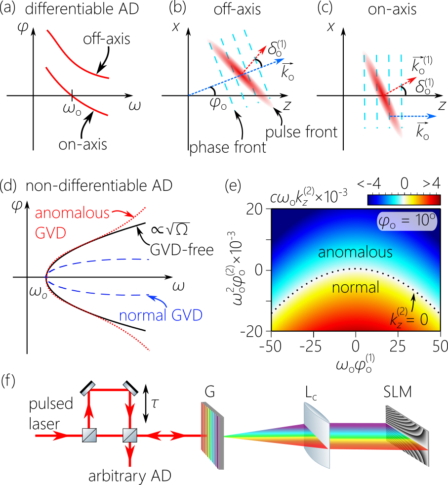
Figure 1: (a) The propagation angle $\varphi(\omega)$ for on-axis and off-axis fields endowed with differentiable AD. (b) Off-axis and (c) on-axis field configurations. (d) Non-differentiable AD enabling GVD-free propagation, normal, or anomalous GVD for on-axis fields. (e) Calculated GVD coefficient $k_{z}^{(2)}$ from Eq. 2 as a function $\omega_{\mathrm{o}}\varphi_{\mathrm{o}}^{(1)}$ and $\omega_{\mathrm{o}}^{2}\varphi_{\mathrm{o}}^{(2)}$ for an off-axis field $\varphi_{\mathrm{o}}\!=\!10^{\circ}$. (f) Setup for realizing arbitrary AD profiles. G: Diffraction grating; L_c: cylindrical lens; SLM: spatial light modulator.

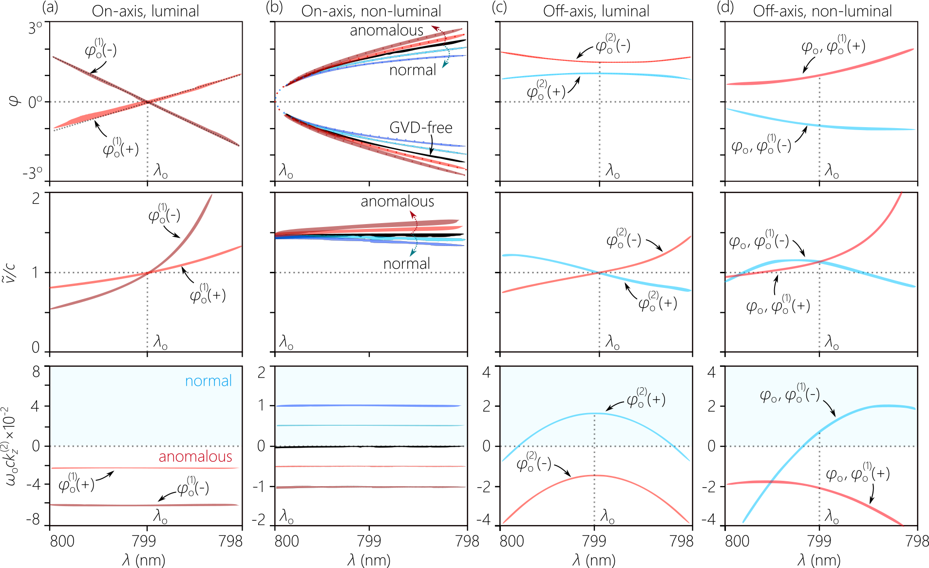
Figure 2: Measurements of the propagation angle $\varphi(\lambda)$ in the first row, from which we extract the group velocity $\widetilde{v}(\lambda)\!=\!(k_{z}(\lambda)-k_{\mathrm{o}})/\Omega$ in the second row, and the GVD coefficient $k_{z}^{(2)}(\lambda)\!=\!2(k_{z}(\lambda)-k_{\mathrm{o}}-\Omega/\widetilde{v})/\Omega^{2}$ in the third row. The red curves correspond to anomalous GVD and the blue to normal GVD. (a) On-axis ($\varphi_{\mathrm{o}}\!=\!0$) luminal ($\widetilde{v}\!=\!c$) fields, with $\lambda_{\mathrm{o}}\!=\!799$ nm, and $\omega_{\mathrm{o}}\varphi^{(1)}_{\mathrm{o}}\!=\!10$ and $-25$. The GVD is anomalous in both cases. (b) Non-differentiable AD from Eq. 3 producing normal and anomalous GVD in on-axis fields with $\widetilde{v}\!=\!1.5c$, and $\omega_{\mathrm{o}}ck_{z}^{(2)}\!=\!\pm 50$, $\pm 100$, and 0 (GVD-free, black curve in the center). Propagation angles $\varphi\!\approx\!0^{\circ}$ are blocked by a spatial filter that removes the zero diffraction order, and the dotted curve is the theoretical prediction. (c) Off-axis luminal fields with $(\varphi_{\mathrm{o}},\omega_{\mathrm{o}}\varphi^{(1)}_{\mathrm{o}},\omega_{\mathrm{o}}^{2}\varphi^{(2)}_{\mathrm{o}})\!=\!(1^{\circ},-8.72\!\times\!10^{-3},-10^{4})$ in blue for normal GVD and $(1.5^{\circ},-1.3\!\times\!10^{-2},10^{4})$ in red for anomalous GVD. (d) Off-axis non-luminal fields with $(-1^{\circ},-8.72,10^{4})$ in blue for normal GVD and $(1^{\circ},8.72,10^{4})$ in red for anomalous GVD.

For off-axis fields, on the other hand, differentiable AD suffices to achieve normal GVD. Porras et al. in [13] propose setting $\varphi_{\mathrm{o}}^{(1)}\!=\!0$ in Eq. 1 and Eq. 2, whereupon $\widetilde{v}\!=\!c/\cos{\varphi_{\mathrm{o}}}$ and $c\omega_{\mathrm{o}}k_{z}^{(2)}\!=\!-\omega_{\mathrm{o}}^{2}\varphi_{\mathrm{o}}^{(2)}\sin{\varphi_{\mathrm{o}}}$, whose sign is determined by $\varphi_{\mathrm{o}}$ and $\varphi_{\mathrm{o}}^{(2)}$. More generally, normal GVD can be realized by judicious choice of $\varphi_{\mathrm{o}}$, $\varphi_{\mathrm{o}}^{(1)}$, and $\varphi_{\mathrm{o}}^{(2)}$, as is clear from Fig. 1(e). Although there always exist normal- and anomalous-GVD regions, the normal-GVD domain shrinks as $\varphi_{\mathrm{o}}\!\rightarrow\!0$. Off-axis fields exhibiting normal GVD may have $\widetilde{v}\!\neq\!c$ (as in [13]) or $\widetilde{v}\!=\!c$, the latter of which requires satisfying the constraint $\varphi_{\mathrm{o}}\!=\!-2\delta_{\mathrm{o}}^{(1)}$. In general, producing normal GVD in an off-axis field requires independent control over the first three AD terms $\varphi_{\mathrm{o}}$, $\varphi_{\mathrm{o}}^{(1)}$, and $\varphi_{\mathrm{o}}^{(2)}$. Conventional optical components such as gratings and prisms do not offer such tailored control; indeed, gratings produce solely anomalous GVD. Finally, the higher-order dispersion coefficients $k_{z}^{(n)}$ for $n\!>\!2$ are not eliminated in off-axis fields endowed with differentiable AD as they are in on-axis fields endowed with non-differentiable AD.

In our experiments, we make use of the arrangement depicted in Fig. 1(f) that can introduce arbitrary AD profiles $\varphi(\omega)$, whether differentiable or non-differentiable. This pulsed-beam shaper comprises a diffraction grating and a cylindrical lens to spatially resolve and collimate the spectrum of plane-wave femtosecond pulses (Tsnumai, Spectra Physics; wavelength $\approx\!800$ nm, bandwidth $\approx\!10$ nm, and pulsewidth $\sim\!100$ fs). A reflective, phase-only SLM placed at the focal plane modulates the phase of the impinging spectrally resolved wave front. Each wavelength $\lambda$ occupies a column on the SLM, and a phase of the form $\tfrac{2\pi}{\lambda}x\sin{\varphi(\lambda)}$ deflects it at a prescribed angle $\varphi(\lambda)$ with respect to the $z$-axis. Because the SLM implements the angle $\varphi$ independently for each $\lambda$, arbitrary functional forms for $\varphi(\lambda)$ can be produced in principle. We record $\varphi(\lambda)$ by taking a spatial Fourier transform of the spectrally resolved wave front.

We first introduce differentiable AD into on-axis fields $\varphi_{\mathrm{o}}\!=\!0$ with $\varphi_{\mathrm{o}}^{(1)}$ taking on positive and negative values [Fig. 2(a)]; i.e., $\varphi(\omega_{\mathrm{o}}+\Omega)\!=\!\varphi_{\mathrm{o}}^{(1)}\Omega$, with $\lambda_{\mathrm{o}}\!=\!799$ nm. This approximates the AD produced by a grating after eliminating higher-order AD terms $\varphi_{\mathrm{o}}^{(n)}\!=\!0$ for $n\!\geq\!2$ (see also [31, 32]). The GVD is anomalous whether $\varphi_{\mathrm{o}}^{(1)}$ is positive or negative, and $\widetilde{v}\!=\!c$ at $\lambda_{\mathrm{o}}$. Because $\varphi$ is purely linear in $\Omega$, the GVD is spectrally flat. In general, this is the domain of validity of the MGF result: on-axis luminal fields endowed with differentiable AD.

We next examine the possibility of realizing normal GVD in an on-axis field, which necessitates introducing non-differentiable AD. We show in Fig. 2(b) measurements for 5 on-axis fields whose AD are implemented according to Eq. 3 and are thus endowed with non-differentiable AD. In all cases, the field is non-luminal with $\widetilde{v}\!=\!1.5c$ and $\lambda_{\mathrm{o}}\!=\!800$ nm. The central field (shown in black) is GVD-free with $\varphi(\omega)\!\approx\!\eta\sqrt{\tfrac{\Omega}{\omega_{\mathrm{o}}}}$. Besides this field, we produce two anomalous-GVD fields $c\omega_{\mathrm{o}}k_{2}\!=\!-50$ and -100, and two normal-GVD fields with $c\omega_{\mathrm{o}}k_{2}\!=\!50$ and 100. Normal and anomalous GVD are produced here symmetrically, independently of $\widetilde{v}$. The group velocities $\widetilde{v}(\lambda)$ for all 5 fields are linear in $\lambda$ over the bandwidth used ($\Delta\lambda\!\approx\!2$ nm), except for the GVD-free field in which $\widetilde{v}(\lambda)$ is independent of $\lambda$. Consequently, $k_{z}^{(2)}$ is a wavelength-independent constant in all cases.

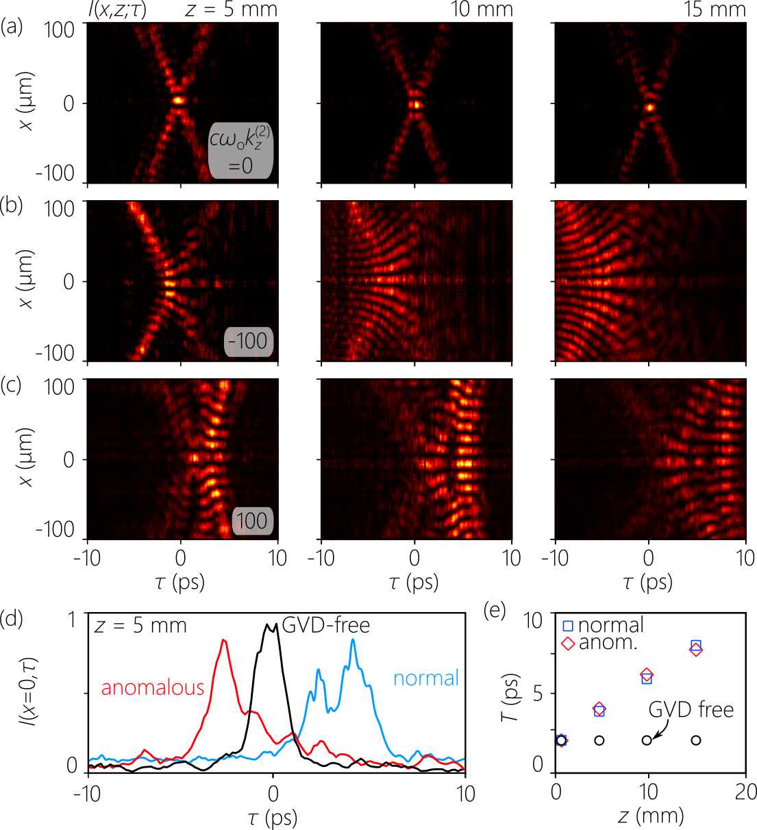
Figure 3: Measured spatio-temporal profiles $I(x,z;\tau)$ all with $\widetilde{v}\!=\!1.5c$ at $z\!=\!5$, 10, and 15 mm, for (a) a propagation-invariant GVD-free field, (b) after introducing anomalous GVD $\omega_{\mathrm{o}}ck_{z}^{(2)}\!=\!-100$, and (c) normal GVD $\omega_{\mathrm{o}}ck_{z}^{(2)}\!=\!100$, all from Fig. 2(b); see Eq. 3. At $z\!=\!0$, all three fields are identical to that in the first panel in (a). (d) The on-axis $x\!=\!0$ temporal profiles $I(0,z;\tau)$ from (a-c) at $z\!=\!5$ mm. (e) The temporal width $T$ along $z$ for the on-axis fields in (a-c).

The third class of fields are off-axis ($\varphi_{\mathrm{o}}\!=\!1^{\circ}$) luminal configurations with $\lambda_{\mathrm{o}}\!=\!799$ nm. We control the sign of the GVD term and set $\widetilde{v}\!=\!c$ by precisely tailoring the values of $\varphi_{\mathrm{o}}$, $\varphi_{\mathrm{o}}^{(1)}$, and $\varphi_{\mathrm{o}}^{(2)}$. Setting $\delta_{\mathrm{o}}^{(1)}\!=\!-\tfrac{1}{2}\varphi_{\mathrm{o}}$ dictates that $\omega_{\mathrm{o}}\varphi_{\mathrm{o}}^{(1)}\!=\!\tan{\delta_{\mathrm{o}}^{(1)}}\!=\!-8.72\!\times\!10^{-3}$ to ensure that $\widetilde{v}\!=\!c$. The GVD coefficient is then tuned by varying the second-order AD term $\omega_{\mathrm{o}}^{2}\varphi_{\mathrm{o}}^{(2)}$. Here we use $\omega_{\mathrm{o}}^{2}\varphi_{\mathrm{o}}^{(2)}\!=\!10^{4}$ to produce anomalous GVD across the spectral range of interest, and $\omega_{\mathrm{o}}^{2}\varphi_{\mathrm{o}}^{(2)}\!=\!-10^{4}$ to produce normal GVD [Fig. 2(c)]. The contribution from the $\omega_{\mathrm{o}}^{2}\varphi_{\mathrm{o}}^{(2)}$ term dominates here over that from $\omega_{\mathrm{o}}\varphi_{\mathrm{o}}^{(1)}$, so that this scenario approaches the proposal by Porras et al. in [13], except that $\omega_{\mathrm{o}}\varphi_{\mathrm{o}}^{(1)}$ deviates slightly from 0 to adjust $\widetilde{v}$ from $c/\cos{\varphi_{\mathrm{o}}}$ to $c$.

Finally, by removing the constraint $\varphi_{\mathrm{o}}\!=\!-\tfrac{1}{2}\delta_{\mathrm{o}}^{(1)}$, the off-axis field is no longer luminal $\widetilde{v}\!\neq\!c$, and we can use the AD terms $\varphi_{\mathrm{o}}$, $\omega_{\mathrm{o}}\varphi_{\mathrm{o}}^{(1)}$ and $\omega_{\mathrm{o}}^{2}\varphi_{\mathrm{o}}^{(2)}$ to adjust the GVD [Fig. 2(d)]. We first consider a field in which $\varphi_{\mathrm{o}}\!=\!-1^{\circ}$, $\omega_{\mathrm{o}}\varphi_{\mathrm{o}}^{(1)}\!=\!-8.72$ and $\omega_{\mathrm{o}}^{2}\varphi_{\mathrm{o}}^{(2)}\!=\!10^{4}$ at $\lambda_{\mathrm{o}}\!=\!799$ nm. Because of the significant value of $\omega_{\mathrm{o}}\varphi_{\mathrm{o}}^{(1)}$ the field is no longer luminal, $\widetilde{v}\!\approx\!1.18c$, and the GVD is anomalous throughout. In another example we set $\varphi_{\mathrm{o}}\!=\!1^{\circ}$, $\omega_{\mathrm{o}}\varphi_{\mathrm{o}}^{(1)}\!=\!8.72$, and $\omega_{\mathrm{o}}^{2}\varphi_{\mathrm{o}}^{(2)}\!=\!10^{4}$. Switching the signs of both $\varphi_{\mathrm{o}}$ and $\omega_{\mathrm{o}}\varphi_{\mathrm{o}}^{(1)}$ while keeping their amplitudes constant retains $\widetilde{v}\!\approx\!1.18c$, but renders the GVD normal over part of the spectrum, as can be verified in Eq. 2. Because $\varphi$ is not linear in terms of $\Omega$ in Fig. 2(c,d), the GVD is not spectrally flat.

The AD-driven GVD in free space was further verified by measuring the spatio-temporal profile of the field $I(x,z;\tau)$ along the $z$-axis by embedding the angular-dispersion synthesizer in one arm of a Mach Zehnder interferometer and placing an optical delay $\tau$ in the reference path for the original laser pulses [Fig. 1(f)]. Scanning the delay $\tau$ produces spatially resolved fringes when the synthesized field overlaps with the reference pulse in space and time. We thus reconstruct $I(x,z;\tau)$ from the interference visibility in a frame moving at $\widetilde{v}\!=\!c/\widetilde{n}$ (see [33, 34, 28] for details). We plot in Fig. 3 measurements for three fields from Fig. 2(b) at $z\!=\!5$, 10, and 15 mm: a propagation-invariant GVD-free field in which $\varphi(\omega)\!\propto\!\sqrt{\Omega}$ [Fig. 3(a)], and fields having anomalous [Fig. 3(b)] and normal GVD [Fig. 3(c)], which both disperse temporally, but in different directions with respect to the leading edge of the initial pulse. The on-axis pulse profiles [Fig. 3(d)] and the pulse widths along $z$ [Fig. 3(e)] both confirm the expected dispersive propagation characteristics of these two fields.

In conclusion, we have shown that the well-known result by MGF [12] implying that AD in free space yields only anomalous GVD applies in fact to only a subset of pulsed optical fields; namely, to on-axis luminal fields incorporating differentiable AD. We have demonstrated here theoretically and experimentally that normal and anomalous GVD can both be produced via AD in on-axis fields via non-differentiable AD (at non-luminal group velocities), and in off-axis fields via differentiable AD (at either luminal or non-luminal group velocities) that requires independent tunability of the first- and second-order AD terms. These results expand the repertoire of applications that can be broached by AD in the areas of dispersion compensation, pulse compression, and nonlinear optics, especially at long wavelengths where material dispersion is anomalous. Both differentiable and non-differentiable AD can be synthesized in the mid-infrared [35] by exploiting appropriate phase plates [36, 37]. In addition, our results are a crucial step towards realizing linear propagation-invariant wave packets in the anomalous dispersion regime [15, 17, 16, 18, 38].

Funding

U.S. Office of Naval Research (ONR) contract N00014-17-1-2458 and ONR MURI contract N00014-20-1-2789.

Disclosures. The authors declare no conflicts of interest.

References

- Torres et al. [2010] J. P. Torres, M. Hendrych, and A. Valencia, Angular dispersion: an enabling tool in nonlinear and quantum optics, Adv. Opt. Photon. 2, 319 (2010).
- Fülöp and Hebling [2010] J. A. Fülöp and J. Hebling, Applications of tilted-pulse-front excitation, in Recent Optical and Photonic Technologies, edited by K. Y. Kim (InTech, 2010).
- Fork et al. [1984] R. L. Fork, O. E. Martinez, and J. P. Gordon, Negative dispersion using pairs of prisms, Opt. Lett. 9, 150 (1984).
- Gordon and Fork [1984] J. P. Gordon and R. L. Fork, Optical resonator with negative dispersion, Opt. Lett. 9, 153 (1984).
- Lemoff and Barty [1993] B. E. Lemoff and C. P. J. Barty, Quintic-phase-limited, spatially uniform expansion and recompression of ultrashort optical pulses, Opt. Lett. 18, 1651 (1993).
- Kane and Squier [1997] S. Kane and J. Squier, Grism-pair stretcher–compressor system for simultaneous second- and third-order dispersion compensation in chirped-pulse amplification, J. Opt. Soc. Am. B 14, 661 (1997).
- Hebling et al. [2002] J. Hebling, G. Almási, I. Z. Kozma, and J. Kuhl, Velocity matching by pulse front tilting for large-area THz-pulse generation, Opt. Express 10, 1161 (2002).
- Szatmari et al. [1990] S. Szatmari, G. Kuhnle, and P. Simon, Pulse compression and traveling wave excitation scheme using a single dispersive element, Appl. Opt. 29, 5372 (1990).
- Szatmári et al. [1996] S. Szatmári, P. Simon, and M. Feuerhake, Group-velocity-dispersion-compensated propagation of short pulses in dispersive media, Opt. Lett. 21, 1156 (1996).
- Sõnajalg and Saari [1996] H. Sõnajalg and P. Saari, Suppression of temporal spread of ultrashort pulses in dispersive media by bessel beam generators, Opt. Lett. 21, 1162 (1996).
- Sõnajalg et al. [1997] H. Sõnajalg, M. Rätsep, and P. Saari, Demonstration of the Bessel-X pulse propagating with strong lateral and longitudinal localization in a dispersive medium, Opt. Lett. 22, 310 (1997).
- Martinez et al. [1984] O. E. Martinez, J. P. Gordon, and R. L. Fork, Negative group-velocity dispersion using refraction, J. Opt. Soc. Am. A 1, 1003 (1984).
- Porras et al. [2003] M. A. Porras, G. Valiulis, and P. Di Trapani, Unified description of Bessel X waves with cone dispersion and tilted pulses, Phys. Rev. E 68, 016613 (2003).
- Zamboni-Rached et al. [2003] M. Zamboni-Rached, K. Z. Nóbrega, H. E. Hernández-Figueroa, and E. Recami, Localized superluminal solutions to the wave equation in (vacuum or) dispersive media, for arbitrary frequencies and with adjustable bandwidth, Opt. Commun. 226, 15 (2003).
- Longhi [2003] S. Longhi, Spatial-temporal Gauss-Laguerre waves in dispersive media, Phys. Rev. E 68, 066612 (2003).
- Longhi [2004] S. Longhi, Localized subluminal envelope pulses in dispersive media, Opt. Lett. 29, 147 (2004).
- Porras and Di Trapani [2004] M. A. Porras and P. Di Trapani, Localized and stationary light wave modes in dispersive media, Phys. Rev. E 69, 066606 (2004).
- Malaguti et al. [2008] S. Malaguti, G. Bellanca, and S. Trillo, Two-dimensional envelope localized waves in the anomalous dispersion regime, Opt. Lett. 33, 1117 (2008).
- Hall et al. [2021a] L. A. Hall, M. Yessenov, and A. F. Abouraddy, Space-time wave packets violate the universal relationship between angular dispersion and pulse-front tilt, Opt. Lett. 46, 1672 (2021a).
- Yessenov et al. [2021] M. Yessenov, L. A. Hall, and A. F. Abouraddy, Engineering the optical vacuum: Arbitrary magnitude, sign, and order of dispersion in free space using space-time wave packets, arXiv:2102.09443 (2021).
- Kondakci and Abouraddy [2016] H. E. Kondakci and A. F. Abouraddy, Diffraction-free pulsed optical beams via space-time correlations, Opt. Express 24, 28659 (2016).
- Parker and Alonso [2016] K. J. Parker and M. A. Alonso, The longitudinal iso-phase condition and needle pulses, Opt. Express 24, 28669 (2016).
- Kondakci and Abouraddy [2017] H. E. Kondakci and A. F. Abouraddy, Diffraction-free space-time beams, Nat. Photon. 11, 733 (2017).
- Porras [2017] M. A. Porras, Gaussian beams diffracting in time, Opt. Lett. 42, 4679 (2017).
- Wong and Kaminer [2017] L. J. Wong and I. Kaminer, Ultrashort tilted-pulsefront pulses and nonparaxial tilted-phase-front beams, ACS Photon. 4, 2257 (2017).
- Efremidis [2017] N. K. Efremidis, Spatiotemporal diffraction-free pulsed beams in free-space of the Airy and Bessel type, Opt. Lett. 42, 5038 (2017).
- Yessenov et al. [2019a] M. Yessenov, B. Bhaduri, H. E. Kondakci, and A. F. Abouraddy, Weaving the rainbow: Space-time optical wave packets, Opt. Photon. News 30, 34 (2019a).
- Yessenov et al. [2019b] M. Yessenov, B. Bhaduri, L. Mach, D. Mardani, H. E. Kondakci, M. A. Alonso, G. A. Atia, and A. F. Abouraddy, What is the maximum differential group delay achievable by a space-time wave packet in free space?, Opt. Express 27, 12443 (2019b).
- Yessenov et al. [2019c] M. Yessenov, B. Bhaduri, H. E. Kondakci, and A. F. Abouraddy, Classification of propagation-invariant space-time light-sheets in free space: Theory and experiments, Phys. Rev. A 99, 023856 (2019c).
- Hebling [1996] J. Hebling, Derivation of the pulse front tilt caused by angular dispersion, Opt. Quant. Electron. 28, 1759 (1996).
- Hall and Abouraddy [2021] L. A. Hall and A. F. Abouraddy, Free-space group-velocity dispersion induced in space-time wave packets by V-shaped spectra, Phys. Rev. A 104, 013505 (2021).
- Hall et al. [2021b] L. A. Hall, M. Yessenov, S. A. Ponomarenko, and A. F. Abouraddy, The space-time Talbot effect, APL Photon. 6, 056105 (2021b).
- Kondakci and Abouraddy [2019] H. E. Kondakci and A. F. Abouraddy, Optical space-time wave packets of arbitrary group velocity in free space, Nat. Commun. 10, 929 (2019).
- Bhaduri et al. [2019a] B. Bhaduri, M. Yessenov, and A. F. Abouraddy, Space-time wave packets that travel in optical materials at the speed of light in vacuum, Optica 6, 139 (2019a).
- Yessenov et al. [2020] M. Yessenov, Q. Ru, K. L. Schepler, M. Meem, R. Menon, K. L. Vodopyanov, and A. F. Abouraddy, Mid-infrared diffraction-free space-time wave packets, OSA Continuum 3, 420 (2020).
- Kondakci et al. [2018] H. E. Kondakci, M. Yessenov, M. Meem, D. Reyes, D. Thul, S. R. Fairchild, M. Richardson, R. Menon, and A. F. Abouraddy, Synthesizing broadband propagation-invariant space-time wave packets using transmissive phase plates, Opt. Express 26, 13628 (2018).
- Bhaduri et al. [2019b] B. Bhaduri, M. Yessenov, D. Reyes, J. Pena, M. Meem, S. R. Fairchild, R. Menon, M. C. Richardson, and A. F. Abouraddy, Broadband space-time wave packets propagating 70 m, Opt. Lett. 44, 2073 (2019b).
- Mills et al. [2012] M. S. Mills, G. A. Siviloglou, N. Efremidis, T. Graf, E. M. Wright, J. V. Moloney, and D. N. Christodoulides, Localized waves with spherical harmonic symmetries, Phys. Rev. A 86, 063811 (2012).