SemSegMap – 3D Segment-based Semantic Localization

Abstract

Localization is an essential task for mobile autonomous robotic systems that want to use pre-existing maps or create new ones in the context of SLAM. Today, many robotic platforms are equipped with high-accuracy 3D LiDAR sensors, which allow a geometric mapping, and cameras able to provide semantic cues of the environment. Segment-based mapping and localization have been applied with great success to 3D point-cloud data, while semantic understanding has been shown to improve localization performance in vision based systems. In this paper we combine both modalities in SemSegMap, extending SegMap into a segment based mapping framework able to also leverage color and semantic data from the environment to improve localization accuracy and robustness. In particular, we present new segmentation and descriptor extraction processes. The segmentation process benefits from additional distance information from color and semantic class consistency resulting in more repeatable segments and more overlap after re-visiting a place. For the descriptor, a tight fusion approach in a deep-learned descriptor extraction network is performed leading to a higher descriptiveness for landmark matching. We demonstrate the advantages of this fusion on multiple simulated and real-world datasets and compare its performance to various baselines. We show that we are able to find $50.9\,\mathrm{\%}$ more high-accuracy prior-less global localizations compared to SegMap on challenging datasets using very compact maps while also providing accurate full 6 DoF pose estimates in real-time.

I Introduction

Mobile robots are continuously increasing their impact on our everyday life and becoming more and more viable not only in structured factories but also unstructured environments and in contact with humans [1]. One of the most crucial capabilities of mobile robots is the ability to know their position in the environment in order to navigate and fulfill their task. Positioning can be framed either in the context of localization in a known map or in the context of the Simultaneous Localization and Mapping (SLAM) problem where localizations and potential loop closures are needed to maintain a consistent map. A multitude of solutions to the positioning problem exist, mainly depending on the available sensor data, specific challenges of the environment and computational limitations of the robotic platform [1].

For standard indoor applications, visual localization based on hand-crafted keypoint descriptors [2, 3] has been demonstrated to achieve high accuracy and recall. However, outdoor applications typically pose challenges to those methods, namely large-scale environments, self similarity and vast appearance changes due to weather, daytime and seasonal conditions [4]. Vision based learning methods improve on viewpoint and appearance invariance [5, 6, 7] by enabling a more context aware description. In contrast, Light Detection and Ranging (LiDAR) based localization achieves illumination invariance using geometry to describe the environment [8, 9], however in turn missing rich information available from vision.

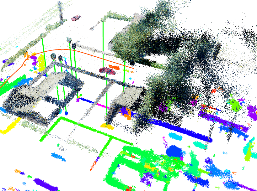
Figure 1: This image shows the SemSegMap pipeline in action. SemSegMap is able to perform segment-based semantic localization on point cloud data enriched with semantic and color information from a visual camera. The currently observed local map around the robot is shown as the colored point cloud on top of the global map depicted below, with each segment having a unique color. Green lines show matched segment correspondences leading to a localization while the orange line shows the robot trajectory.

As a combined solution, in this paper, we introduce SemSegMap, a method that leverages the visual and semantic information available from cameras and fuses it with geometric information from a standard 3D LiDAR. As a basis for our localization framework we use SegMap [8], a LiDAR based SLAM pipeline that uses 3D segments of the environment as landmarks and allows for 6D pose retrieval from compact descriptors in large-scale maps. In contrast to SegMap, in SemSegMap, as outlined in Figure 1, first the point cloud (PC) gets enriched with color and semantic information using back-projection of semantically segmented RGB images. Further, the PC is segmented based on geometric, color and semantic information to create consistent and meaningful segments. We show in multiple experiments that as a result of this fusion, the segmentation process and the generated descriptors become more robust to viewpoint and appearance changes, thus enabling a more consistent re-localization of the robot.

Our contributions are as follow

• We show that integrating color and semantic information from a cameras into PCs improves both the segmentation and descriptor generation processes, leading to more consistent 6D localizations in a SLAM pipeline.

• We introduce a simulation based learning pipeline for training segment descriptors using ground truth associations, and show their transferability to real-world scenarios.

• We demonstrate the performance of SemSegMap in an extensive evaluation on simulation and real-world data outperforming various baselines.

• For the benefit of the community, we open-source the whole framework under a permissive license available at: https://github.com/ethz-asl/segmap.

II Related Work

The ability to localize is at the heart of the SLAM problem [1]. Two distinct problems addressed in localization are the localization of landmarks, which can then be used to calculate a precise 6D location in a global map, and place recognition, where only a rough neighborhood is estimated.

Vision-based place recognition methods such as NetVLAD [7] or DELF [10] have the advantage that they can incorporate a lot of contextual information and thus gain high robustness to viewpoint and illumination changes. Some recent techniques explicitly model the semantics of the scene to obtain higher robustness towards seasonal changes [11, 12, 13]. More precise visual keypoint-based place recognition methods are well studied [14] and of significant interest [15], but they present their own set of challenges with regards to scalability, viewpoint, and illumination changes. A compromise between precise keypoint localization and the ability to incorporate contextual and semantic information can be found in object-based localization frameworks [16, 17].

LiDAR based localization methods rely mainly on matching geometry and can be separated into various categories. Many PC registration methods, out of which Iterative Closest Point (ICP) [18] is the most well-known one, require a good pose prior and are not suited for global localization. While global registration methods exist that work beyond the local context [19, 20], they still require storing at least parts of the PC data. This can be partially mitigated by only extracting compact descriptors during map building and localization. Descriptors of single LiDAR scans [21, 22, 23, 24] only allow rough location estimates and not precise 6D poses that could be integrated into a SLAM pipeline. Descriptors of local keypoint neighborhoods [25, 26, 27, 28] in turn can be noisy and lack distinctiveness due to only having geometry data available. A combination can be achieved by performing a refinement step, e.g. using ICP, after the rough localization, but would again require storing and working with PC data [29, 30].

PC segment description and mapping based approaches were first proposed by Douillard et al. [31] and Nieto et al. [32] and then further extended into a full SLAM pipeline in SegMap by Dubé et al. [8]. SegMap leverages advantages from both local and global descriptors by looking at features in the environment that are large enough to be more robust and meaningful, while also maintaining the ability to produce accurate 6D poses. Extensions to the pipeline include different training methods for the descriptor, as well as fine tuning to different environments [33, 34].

Enriching PCs with semantic information, e.g. obtained by fusing camera and LiDAR data, has proven beneficial [35, 36, 37, 38, 39]. Ratz et al. [40] propose not only to use just one scan instead of an accumulated PC but also to enrich the descriptor with appearance information from a camera using NetVLAD and a customized fusion layer in their network. This increases accuracy at the cost of a significant decrease in computational performance, due to the expensive NetVLAD backbone. Also, the segmentation procedure is still purely based on geometry and cannot incorporate any additional information from the camera. Schönberger et al. [41] propose a localization scheme based on semantically labeled 3D PCs able to localize in the presence of severe viewpoint and appearance changes. They extract a deep-learned descriptor for a subvolume of the semantic map and compare it to similarly extracted ones from a prior map. However, using such submaps only provides a rough place-recognition like localization and require further refinement steps to get 6D poses. Furthermore, by operating on comparably larger subvolumes and the need to check multiple hypothesis, the corresponding descriptor network is computationally expensive.

In contrast, SemSegMap introduces a framework that is both efficient enough to be run in real-time on a consumer CPU (excluding the semantic segmentation running on the GPU) and still able to leverage the rich information available from geometry, appearance and semantics. We perform a very early fusion of the two sensor modalities which allows also the segmentation to be based on all available information.

III SemSegMap

In this section we present the details of the proposed SemSegMap pipeline, as shown in Figure 2.

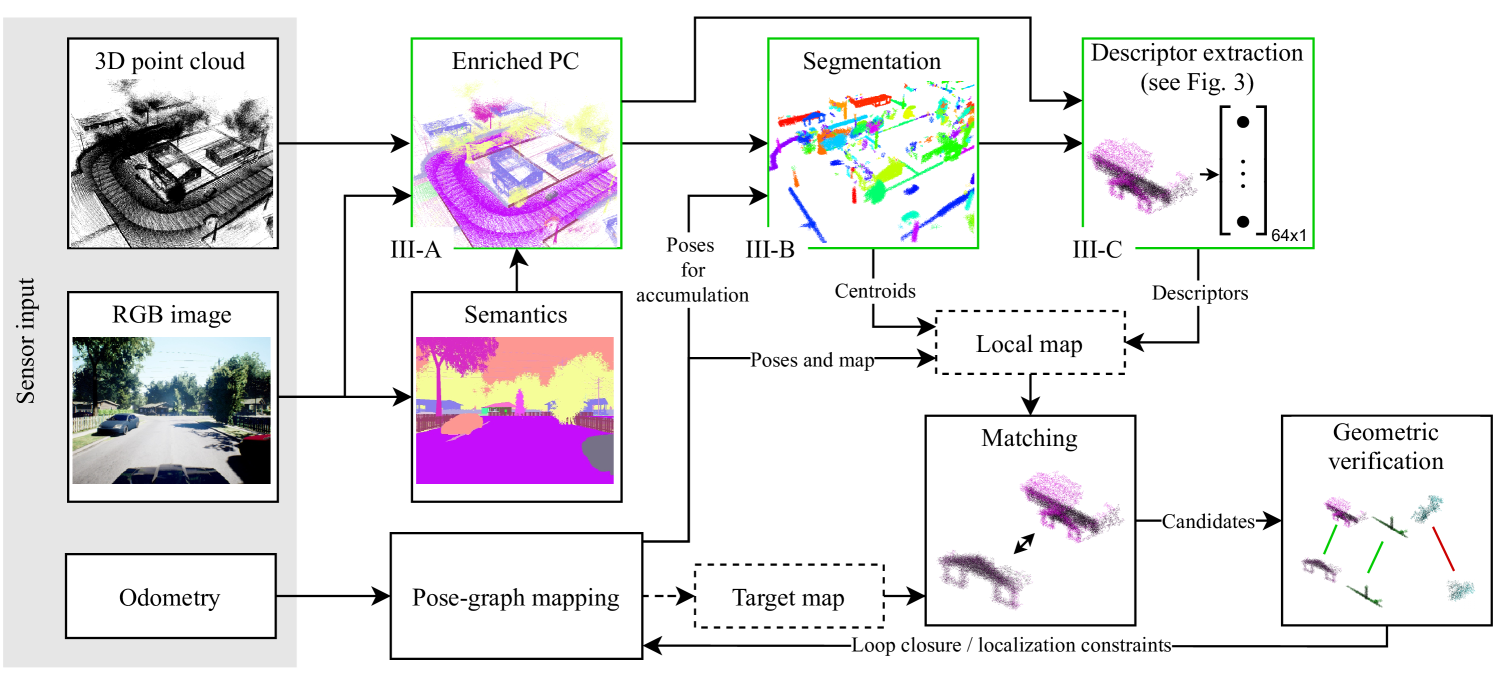
Figure 2: Overview of the SemSegMap pipeline. The whole pipeline can be run in localization mode with a target map loaded from the disk or in loop closure mode where the target map is provided by the current pose-graph. Green: Main modules changed from [8] with corresponding section numbers.

The approach can be split into several key modules, out of which the new segmentation and descriptor explained in Sections III-B and III-C, represent the core contributions of this paper.

III-A Semantic enrichment

The inputs to the pipeline consist of a stream of color images and PCs. The color images are passed through a semantic segmentation network to obtain a semantic class for each pixel. Using the extrinsic calibration between the camera and the LiDAR as well as the intrinsic calibration parameters of the camera, the color and semantic class of each pixel is projected onto the PC. The result is a set of enriched points in the form $\mathbf{p}=\{x,y,z,h,s,v,c\}$, where $x$, $y$, and $z$ are the spatial coordinates, featuring also color values $h$, $s$, and $v$ in HSV space (result visible in Figure 1), and semantic class labels $c$ (example depicted in Figure 2: Enriched PC).

III-B Semantic segmentation

To remove noise and achieve a more compact data representation, we accumulate the enriched PC data in a fixed size voxel grid. The voxel grid is a cylinder with a radius of $R$ that dynamically follows the robot and is centered on it. For each voxel, the color information of multiple points is fused by using a running average over the incoming values to obtain the current value for the voxel. In contrast, the semantic class labels can not be averaged, and therefore, all values are stored and the semantic label of the voxel is determined by majority voting. Further filtering can be done by excluding points that belong to known dynamic classes e.g. humans and cars.

We use an incremental Euclidean segmentation that does not need to be rerun on the entire PC at each step, but is computed incrementally only on the newly active voxels, as detailed in [8]. A segment $\mathcal{S}$ is defined as a set of points, where for each point $\mathbf{p}_{1}\in\mathcal{S}$ there exists at least one other point $\mathbf{p}_{2}\in\mathcal{S}$, so that the distance between these two points is smaller than the segmentation distance $d_{segment}$.

To include the semantic and color information into the segmentation process, we modify the standard Euclidean distance function between two points $\mathbf{p}_{1}$ and $\mathbf{p}_{2}$ to be

$$\begin{split}d^{2}=&\ (x_{1}-x_{2})^{2}+(y_{1}-y_{2})^{2}+(z_{1}-z_{2})^{2}+\\ &f_{h}^{2}(|h_{1}-h_{2}|)+f_{c}^{2}(c_{1},c_{2}).\end{split}$$ (1)

The function $f_{h}$ is used to compute the distance between two colors by only comparing the difference in hue values in order to mitigate the appearance variance and is defined as

$$f_{h}(\Delta h)=\begin{cases*}p_{h}&$\min{(\Delta h,1-\Delta h)}>t_{h}$\\ 0&\text{otherwise}\end{cases*},$$ (2)

where $p_{h}$ is a fixed penalty for when the color difference is above a certain chosen threshold $t_{h}$ and where the hue values $h$ are normalized to $[0,1)$. In practice, there are two cases because the hue color space is cyclical. Similarly, the semantic class distance function is defined as

$$f_{c}(c_{1},c_{2})=\begin{cases*}p_{c}&\text{$c_{1}\neq c_{2}$}\\ 0&\text{otherwise}\end{cases*},$$ (3)

where $p_{c}$ is a fixed penalty applied when the semantic classes do not match. Fixed penalties are necessary because the color space and semantic spaces are either not continuous or not numerically comparable to physical distances in space. A soft constraint on the segmentation can be imposed by choosing $p_{h}$ and $p_{c}$ smaller than $d_{segment}$, which means that two points that are sufficiently close in space can still be part of the same segment, even if they have a very different color or class.

During the segmentation process, at each step, the robot extracts a set of segments in the local map around itself. Those segments slowly accumulate points as more observations are made from different viewpoints. Similarly to how a keypoint is tracked, a segment will have multiple accumulated observations. Therefore, the final observation, just before it moves out of the local map neighborhood, will be the most complete one.

III-C Description

For each segment observation, a learned descriptor is calculated and the local map is built by associating each descriptor to the corresponding segment centroid point. For efficiency reasons, we only keep the descriptor of the last and most complete observation of each segment to create the target map for subsequent localizations or loop closures.

The new descriptor network, illustrated in Figure 3, uses the Pointnet++ architecture [42] that is based on hierarchical point set feature learning.

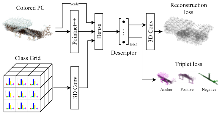
Figure 3: The descriptor extraction of the colored PC is based on a Pointnet++ [42] backbone while the semantics are fused in a coarse voxel grid of semantic class histograms. The network is trained using both a reconstruction loss and a triplet loss.

The input to the Pointnet++ backbone is the colored PC segment that has been randomly subsampled to a fixed size of $2048$ points. The class labels are instead accumulated into a very coarse $3\times 3\times 3$ spatial voxel grid, where each cell contains a normalized histogram of the class labels that fall inside that section of the PC segment. This very coarse description is enough because due to the semantic segmentation process the class labels inside most segments are relatively homogeneous. For the sake of computational efficiency this class representation is handled separately by a small 3D convolutional network, whose output is later concatenated with that of the Pointnet++ backbone. Finally, we also input into the network the scaling factor by which the point coordinates were normalized, which helps the network better discriminate between segments that do not match but are either visually or geometrically similar.

The descriptor is trained using both a triplet loss as well as a reconstruction loss from a convolutional decoder. The triplet loss is formulated as

$$L_{\text{triplet}}=\max(m+\sigma(\mathcal{A},\mathcal{P})\cdot D_{\mathcal{A},\mathcal{P}}-D_{\mathcal{A},\mathcal{N}},0)$$ (4)

where $m=0.4$ is the margin, $D_{\mathcal{A},\mathcal{P}}$ is the Euclidean distance between an anchor segment $\mathcal{A}$ and a positive example $\mathcal{P}$, $D_{\mathcal{A},\mathcal{N}}$ is the Euclidean distance between the anchor and a negative example $\mathcal{N}$, and $\sigma(\mathcal{A},\mathcal{P})=\frac{\mathbf{card}(\mathcal{P})}{\mathbf{card}(\mathcal{A})}$ is the ratio in number of points between anchor and positive example. The scaling $\sigma(\mathcal{A},\mathcal{P})$ is a heuristic that prevents the loss function from penalizing too much segment observations that should match, but due to segment incompleteness only share a small overlap and therefore in practice are hard to match. For the reconstruction loss we use a binary cross entropy loss applied to each voxel. This enables approximate reconstructions of the PC map from only the descriptor space for visualization and improves the descriptor quality of very similar looking segments. During training we augment the PCs in multiple ways, including both geometric variations such as random rotations, jitter, scale shifts, missing points or sections, and visual variations such as color shifts or erronous class labels.

III-D Localization and loop closure

To perform localization or loop closure, candidate correspondences are identified between the locally built map of segments and the prior or global map, respectively. The candidates are identified using the descriptors of each locally visible segment and retrieving the $k$ most similar descriptors from the global map. Finally, a geometric verification step is performed based on the centroids of the target and query match candidates to identify the 6  degree of freedom (DoF) transformation that leads to the largest set of inliers using Random Sample Consensus (RANSAC). The resulting transformation can either be used as a localization result when localizing from a previously built map, or as a loop closure constraint in a SLAM scenario. In the latter case, both the loop closure constraint and robot odometry constraints are placed into an online pose graph based on iSAM2 [43].

IV Experiments

In this section, we describe our training procedure and present thorough evaluation of SemSegMap on both simulated and public real-world datasets, demonstrating a superior performance compared to different baselines on segmentation, descriptor quality, and localization accuracy and robustness.

IV-A Datasets

Datasets including visual as well as PC data, spanning large areas and covering different environmental conditions that include semantic annotations are rare and hard to obtain. Therefore, for the data intensive step of descriptor training, we utilize simulated data to be able to quickly produce training data for SemSegMap. Furthermore, simulated datasets provide the opportunity to specifically evaluate our contribution in isolation of sensor noise, state estimation and calibration inaccuracies, and imperfect semantic segmentation. In addition, we demonstrate the transferablility of our approach to a challenging real-world dataset.

IV-A1 Simulation

Photo-realistic simulation is a popular tool for efficiently generating visually rich data with high quality ground truth annotations. Some of the most popular simulation tools in the robotics domain are Gazebo [44], CARLA [45], LGVSL [46] and AirSim [47]. While CARLA and LGVSL focus on autonomous driving scenarios, Gazebo does not provide photorealistic visual output. The datasets used in the following experiments were generated by AirSim using the ”Modular Neighborhood Pack”, a large residential environment. Each dataset consists of RGB image data, a semantic segmentation map for the image, LiDAR PCs as well as odometry information. The image data consists of three cameras, one on each side and a front facing one, spanning a total horizontal Field of View (FoV) of $270\,\mathrm{{}^{\circ}}$. The simulated LiDAR has a resolution of $1920\times 64$ and the same $270\,\mathrm{{}^{\circ}}$ FoV. All sensors are synchronized and operated at $5\,\mathrm{Hz}$.

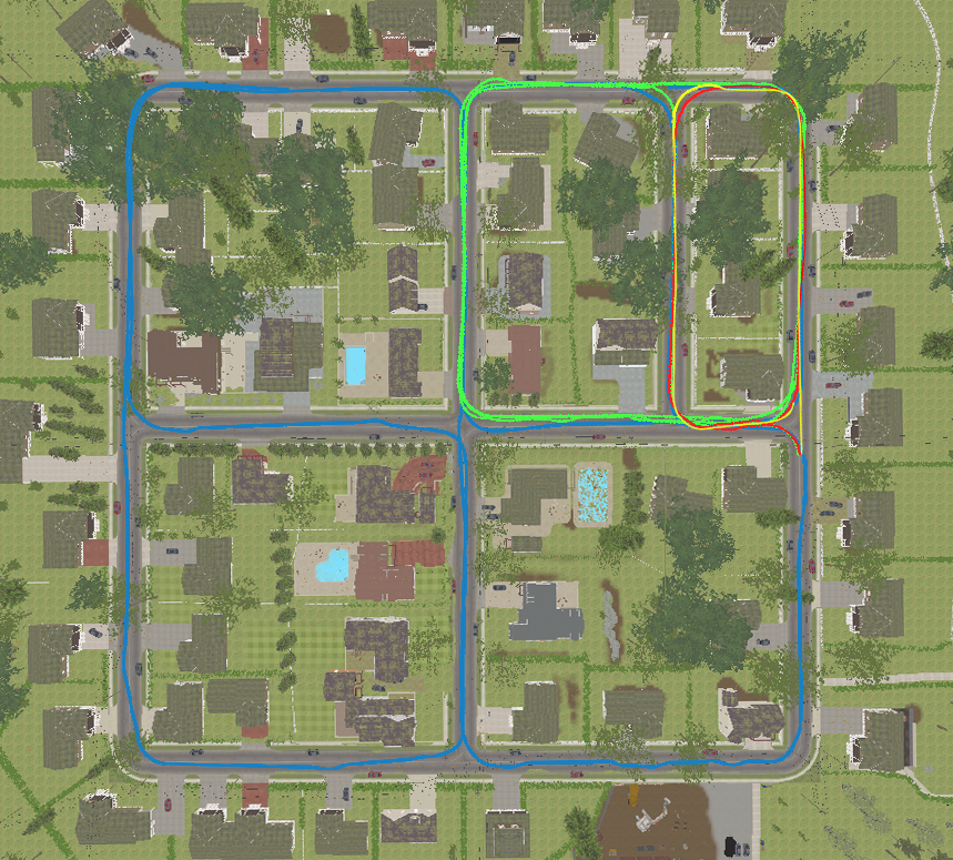
Figure 4: Bird’s eye view of the simulation environment including the simulated trajectories (blue: S0, green: S1, red: S2, yellow: S3).

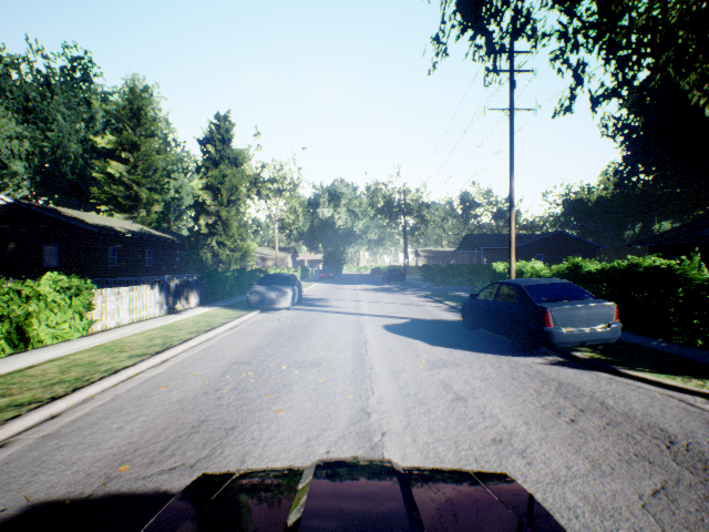
((a)) RGB image: Sunny day

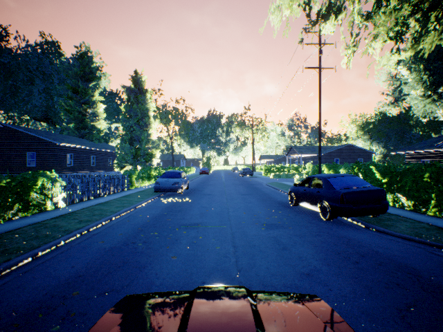
((b)) RGB image: Sunrise

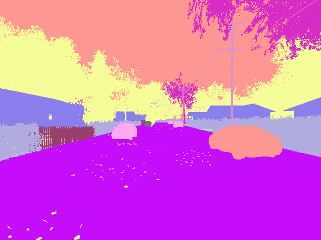
((c)) Semantic segmentation

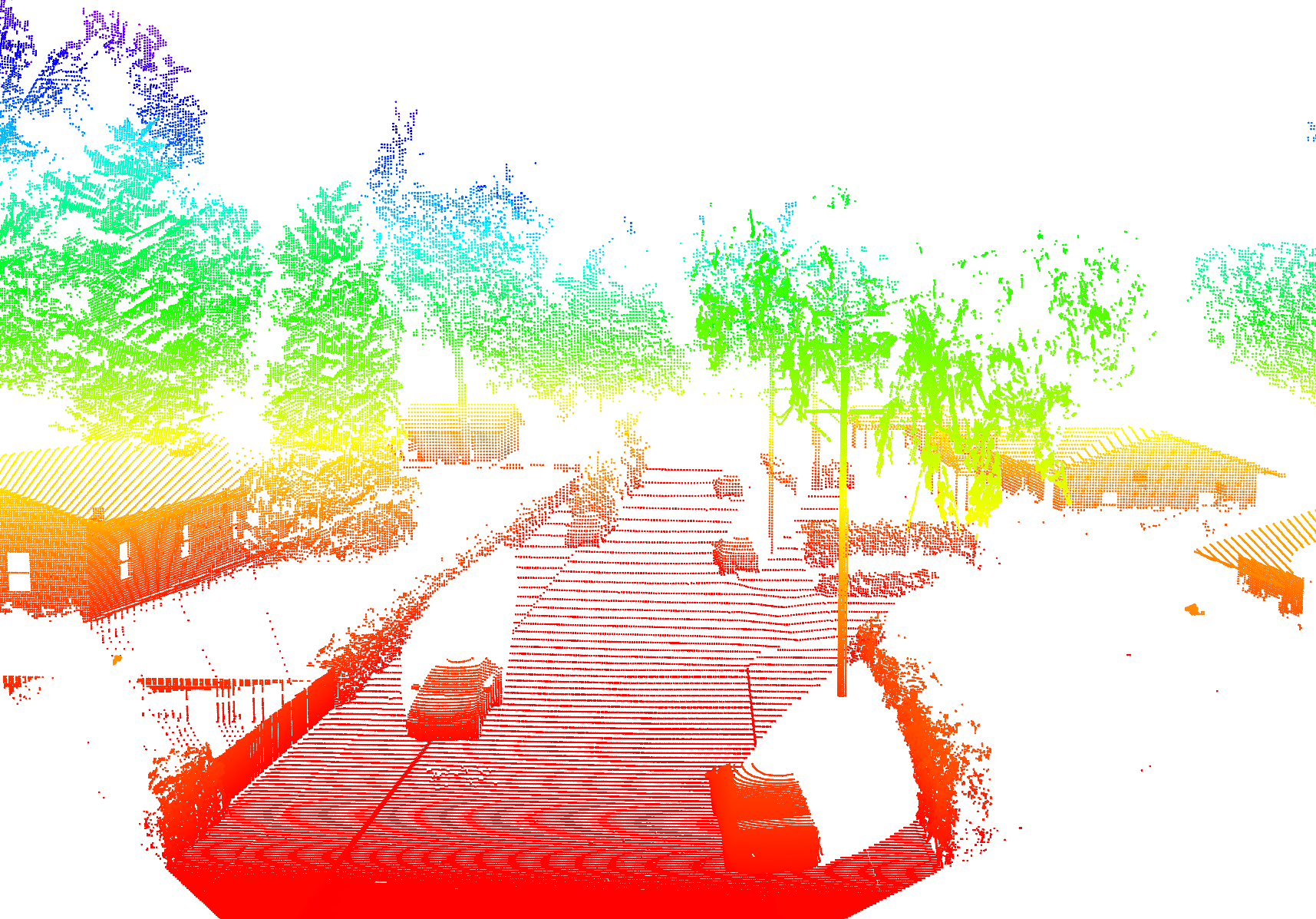
((d)) 3D LiDAR PC

Figure 5: Overview of simulated sensor modalities and environmental conditions.

An overview of the neighborhood, the simulated environmental conditions, as well as the simulated trajectories, is given in Figure 4 and 5, and Table I, respectively.

IV-A2 Real world data

For demonstrating the applicability of our approach to real-world environments, we use the NCLT dataset [48]. The dataset provides raw sensor data from a LiDAR sensor, an omnidirectional camera, and ground truth position data, among others. As the images lack ground-truth semantic labelling, we used the author’s implementation from [49] to semantically segment the images from the five horizontal color cameras. The camera-to-LiDAR extrinsics, provided in the dataset, were used to enrich the PCs with color and semantic information by projection onto the image plane. As a last step, we removed the local ground plane from the enriched PC in order to make the subsequent segmentation process more robust. Because the dataset was recorded on a SegWay, which experiences a lot of back and forth pitching motion, the ground plane cannot simply be removed by setting a height threshold on the raw PC. Instead, we estimated the local ground plane based on the points in the enriched PC whose class labels correspond to ground and subsequently removed all points in close proximity to these points. A subset of the dataset featuring large map overlap and different environmental conditions was processed and used for our experiments as listed in Table II.

TABLE I: Overview of simulated trajectories. The referenced trajectories as well as environmental conditions are shown in Figures 4 and 5, respectively.

#	Length	Conditions	Comment
S0	$2071\,\mathrm{m}$	daytime, sunny, clear	Covers whole map
S1	$1462\,\mathrm{m}$	daytime, sunny, clear	Medium size with overlap
S2	$377\,\mathrm{m}$	daytime, sunny, clear	Single small loop
S3	$358\,\mathrm{m}$	early sunrise, shadows	Opposite direction to S2

TABLE II: Overview of the trajectories extracted from the NCLT dataset. Please refer to [48] for a detailed description of the dataset.

#	Date	Time	Conditions
N0	2012-04-29	$4\,\mathrm{min}-30\,\mathrm{min}$	morning, sunny, foliage
N1	2012-05-26	$0\,\mathrm{min}-10\,\mathrm{min}$	evening, sunny, foliage
N2	2012-11-04	$0\,\mathrm{min}-25\,\mathrm{min}$	morning, cloudy
N3	2013-04-05	$54\,\mathrm{min}-69\,\mathrm{min}$	afternoon, sunny, snow

IV-B Segmentation

To evaluate the segmentation method presented in Section III-B we use the simulation dataset run S1 and the NCLT run N0. For the classic Euclidean segmentation in SegMap we use the default segmentation distance $d_{segment}=0.2$. In SemSegMap we adjust this to $d_{segment}=0.3$ and set the penalties and thresholds in the color and semantic distance functions to $t_{h}=0.1$, $p_{h}=0.05$ and $p_{c}=0.15$.

To measure the segmentation quality, we first calculate the convex hull $V_{i}$ of each segment $S_{i}$ in the local map, and then compare it to the segment $S_{j}$ with the convex hull $V_{j}$ at the same global location in the target map. The quality of the segmentation is then given by the Intersection Over Union (IoU) as

$$\text{IoU}(V_{i},V_{j})=\frac{V_{i}\cap V_{j}}{V_{i}\cup V_{j}}.$$ (5)

In this way, we compare how repeatable and accurate the segmentation is when visiting the same place multiple times. Figure 6 shows the segmentation IoU results from run S1 in the simulated environment which features multiple intersecting loops in the same environment and N0 for the NCLT dataset. A low IoU indicates that the segment was not properly re-segmented when re-visiting the place, while a high IoU corresponds to a consistent re-segmentation. In the latter case the segments occupy the same volume in space and are therefore more likely to be matched based on their descriptors. We consider an $\text{IoU}\geq 0.33$ to represent a good overlap while an $\text{IoU}<0.33$ represents an inconsistent segmentation. SemSegMap produced $-24.24\,\mathrm{\%}$ and $-8.38\,\mathrm{\%}$ less inconsistent segments with $\text{IoU}<0.33$ while obtaining $30.97\,\mathrm{\%}$ and $25.03\,\mathrm{\%}$ more consistent segments with an $\text{IoU}\geq 0.33$ with respect to SegMap for the simulation and NCLT dataset, respectively.

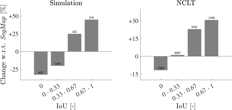
Figure 6: Change of the segmentation IoU for the simulation dataset S1 (left) and NCLT N0 (right) using SemSegMap with respect to SegMap. The bins represent the change in number of segments with a specific IoU range. The small numbers on top of the bars depict the absolute numbers of segments in that range produced by SemSegMap. While SemSegMap produces less segments with low IoU, which represent inconsistent segmentations, it is able to produce more consistent segments with a high overlap and IoU compared to SegMap.

IV-C Descriptor quality

To evaluate the impact of our adapted descriptor extraction network described in Section III-C, we performed a similar experiment as described in [8, Section 5.4].

In order to use the segments as landmarks in a localization and loop-closure scenario as described in Section III-D, we obtain candidate matches using $k$ nearest neighbours ($k$-NN). For a more robust and efficient localization, the amount $k$ of candidates necessary to retrieve the correct match should be as small as possible, even with partially observed segments which occur during live operation or different directions of travel. In Figure 7, we show a comparison of how high $k$ needs to be in order to retrieve the correct match using SemSegMap and different state-of-the-art PC descriptors operating on the simulation dataset S0 and the NCLT dataset N0. The SemSegMap network is trained solely on ground truth data obtained from S1 and not retrained on the NCLT data.

We compare the quality of our descriptor to a learned segment descriptor [8] for the simulated data, and extended the evaluation for the NCLT dataset to the hand-crafted descriptor FPFH [25] and the learned local descriptor 3DSmoothNet [28]. For FPFH, a single segment descriptor was computed by selecting the segment centroid as the keypoint and choosing the descriptor radius to encompass all points of the respective segment [50]. In the case of 3DSmoothNet, simply extending the radius did not yield meaningful results. One reason could be that the descriptor was specifically designed and trained as a local descriptor. In order to deploy it within our segment-based framework, we randomly select points from the segment PC as keypoints, extract local descriptors for each keypoint and aggregate them to a global descriptor by following a bag of words (BoW) approach using $k$-means clustering. Specifically, we trained the $k$-means model on a subset of segments extracted from N0, where $k=16$ yielded the best results.

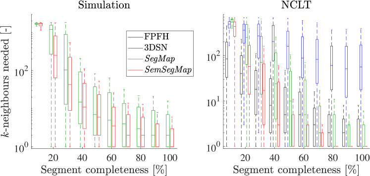
Figure 7: Comparison of descriptor quality on the simulation dataset S0 (left) and the NCLT dataset N0 (right).

Note from Figure 7 that SemSegMap outperforms all other descriptors in both datasets except for FPFH with incomplete segments with completeness $<30\,\mathrm{\%}$. This property of the SemSegMap descriptor is controlled by the $\sigma$ term in the triplet loss formulation introduced in Equation 4 that biases the network towards better matching more complete segments. Removing the influence of this term causes better matching performance for harder matches, i.e. at low completeness thresholds, but at the same time reduces the matching performance of more complete segments as the descriptor attempts to perform more unlikely matches. However, in a typical SLAM application, while an early localization, e.g. with many incomplete segments is important, achieving more accurate and robust localizations during operation with complete segments is often of greater interest in a full smoothing and mapping framework. The descriptor transfers well to the more challenging real-world data from the NCLT dataset, where the performance difference is even more evident.

IV-D Localization accuracy and robustness

To assess the localization accuracy and robustness, we tested SemSegMaps ability to localize in a previously built target map. Therefore, we recorded the target map on trajectories S0 and N0 for the simulation and NCLT dataset, respectively. The map for S0 contains $2006$ segments and has a size of $0.51\,\mathrm{MB}$ while for N0 there are $2588$ segments in a $0.66\,\mathrm{MB}$ map. All other trajectories except for the training set S1 are used for on-line localization against the target map as described in Section III-D.

For the localization evaluation we retrieve a total of 16 neighbours using $k$-NN. For the geometric verification in our experiments the RANSAC was set to require a minimum of $6$ and $7$ inliers for the simulation and NCLT dataset, respectively, and allow a centroid distance of at most $0.4\,\mathrm{m}$. For all the experiments for both SegMap and SemSegMap we keep these parameters fixed and only change the segmentation and description process as outlined in Sections III-A and III-C, to provide the fairest comparison. With these settings SemSegMap (excluding the semantic segmentation) runs on an Intel i7-8700 CPU with an average frequency of $6.13\,\mathrm{Hz}$ and $6.74\,\mathrm{Hz}$ on the simulation and NCLT dataset, respectively.

Table III and Figures 8 and 9 report the accuracy results of the estimated 6-DoF pose for the simulation and NCLT dataset, respectively. SemSegMap is able to consistently find more localizations throughout all the tested datasets. In simulation, less affected by odometry and sensor noise, SemSegMap is able to find a total of $102\,\mathrm{\%}$ more high accuracy localizations (translation error of less than $1\,\mathrm{m}$) with respect to SegMap and $165\,\mathrm{\%}$ more accurate localizations (translation error of less than $5\,\mathrm{m}$). Especially on trajectory S3, SegMap suffers from different appearance and viewpoint while SemSegMap is less affected and still able to produce many accurate localizations. Those results also transfer to the real-world dataset where more than $50.9\,\mathrm{\%}$ high accuracy localization and $24.7\,\mathrm{\%}$ more accurate localizations are found compared to SegMap.

TABLE III: Localization accuracy results overview ($n_{<\bullet\,\mathrm{m}}$ relative improvement of SemSegMap with respect to SegMap with a certain accuracy).

#	Number of localizations		$n_{<1\,\mathrm{m}}$	$n_{<5\,\mathrm{m}}$
	SegMap	SemSegMap
S2	126	258	53.93 %	100.79 %
S3	10	108	4400 %	980 %
N1	1201	1395	60.00 %	14.96 %
N2	1060	1337	44.17 %	27.55 %
N3	774	1056	41.70 %	35.58 %

V Conclusions

In this paper, we introduced SemSegMap, an extension to SegMap that fuses both color and semantic information from an RGB camera with LiDAR data in real-time. In a real-world robotic application, the addition of cameras to a platform equipped with a LiDAR is typically easily possible due to the comparably low price of cameras and their cross-purpose use, especially when also performing semantic segmentation to improve scene understanding. We include this additional modality both to improve segmentation and descriptor quality, which we showed in a stimulated dataset with accurate ground truth and a challenging real-world dataset.

Using the described extensions, SemSegMap is able to outperform a geometric segmentation approach by producing less inconsistent segments and more highly overlapping segments when re-visiting a place. The tight fusion of the additional information in the descriptor also increases descriptor quality where SemSegMap not only outperforms the SegMap baseline but also other state-of-the-art PC descriptors like FPFH and 3DSmoothNet in terms of $k$-NN required to find the correct match. These improvements also propagate to the localization accuracy and robustness resulting in SemSegMap providing $102\,\mathrm{\%}$ and $50.9\,\mathrm{\%}$ more high accuracy localizations than SegMap for the simulated and the real-world dataset, respectively.

To further extend our framework, a combination of FPFH and SemSegMap descriptor based on the expected completeness of a segment could be used in order to benefit from both advantages.

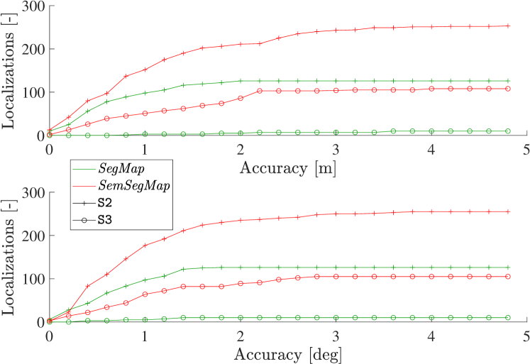
Figure 8: Cumulative successful localizations with a certain accuracy on the simulation datasets with a target map built from S0.

Figure 9: Cumulative successful localizations with a certain accuracy on the real-world datasets with a target map built from N0.

GNSS

Global Navigation Satellite System

IMU

Inertial Measurement Unit

SLAM

Simultaneous Localization and Mapping

MAV

Micro Aerial Vehicle

FoV

Field of View

RTK

Real-Time Kinematic

RMSE

Root Mean Square Error

LiDAR

Light Detection and Ranging

ICP

Iterative Closest Point

$k$-NN

$k$ nearest neighbours

DoF

degree of freedom

RANSAC

Random Sample Consensus

IoU

Intersection Over Union

PC

point cloud

BoW

bag of words

References

- [1] C. Cadena, L. Carlone, H. Carrillo, Y. Latif, D. Scaramuzza, J. Neira, I. Reid, and J. J. Leonard, “Past, Present, and Future of Simultaneous Localization and Mapping: Toward the Robust-Perception Age,” IEEE Transactions on Robotics, vol. 32, no. 6, Dec. 2016.
- [2] T. Schneider, M. Dymczyk, M. Fehr, K. Egger, S. Lynen, I. Gilitschenski, and R. Siegwart, “maplab: An Open Framework for Research in Visual-inertial Mapping and Localization,” IEEE Robotics and Automation Letters, vol. 3, no. 3, 11 2018.
- [3] R. Mur-Artal, J. M. M. Montiel, and J. D. Tardos, “ORB-SLAM: A Versatile and Accurate Monocular SLAM System,” IEEE Transactions on Robotics, vol. 31, no. 5, 10 2015.
- [4] M. J. Milford and G. F. Wyeth, “SeqSLAM: Visual route-based navigation for sunny summer days and stormy winter nights,” in IEEE International Conference on Robotics and Automation (ICRA), 2012.
- [5] J. Revaud, P. Weinzaepfel, C. R. de Souza, and M. Humenberger, “R2D2: repeatable and reliable detector and descriptor,” in Advances in Neural Information Processing Systems, 2019.
- [6] P.-E. Sarlin, C. Cadena, R. Siegwart, and M. Dymczyk, “From Coarse to Fine: Robust Hierarchical Localization at Large Scale,” in IEEE Computer Society Conference on Computer Vision and Pattern Recognition, Dec. 2018.
- [7] R. Arandjelović, P. Gronat, A. Torii, T. Pajdla, and J. Sivic, “NetVLAD: CNN Architecture for Weakly Supervised Place Recognition,” IEEE Transactions on Pattern Analysis and Machine Intelligence, vol. 40, no. 6, 2018.
- [8] R. Dubé, A. Cramariuc, D. Dugas, H. Sommer, M. Dymczyk, J. Nieto, R. Siegwart, and C. Cadena, “SegMap: Segment-based mapping and localization using data-driven descriptors,” The International Journal of Robotics Research, vol. 39, no. 2-3, 2019.
- [9] M. Elhousni and X. Huang, “A Survey on 3D LiDAR Localization for Autonomous Vehicles,” in 2020 IEEE Intelligent Vehicles Symposium (IV2020), Las Vegas, US, May 2020.
- [10] H. Noh, A. Araujo, J. Sim, T. Weyand, and B. Han, “Large-Scale Image Retrieval with Attentive Deep Local Features,” in 2017 IEEE International Conference on Computer Vision (ICCV), Oct. 2017.
- [11] A. Gawel, C. Del Don, R. Siegwart, J. Nieto, and C. Cadena, “X-View: Graph-Based Semantic Multi-View Localization,” IEEE Robotics and Automation Letters, vol. 3, no. 3, 2017.
- [12] A. Benbihi, S. Arravechia, M. Geist, and C. Pradalier, “Image-Based Place Recognition on Bucolic Environment Across Seasons From Semantic Edge Description,” in 2020 IEEE International Conference on Robotics and Automation (ICRA), 2020.
- [13] H. Hu, Z. Qiao, M. Cheng, Z. Liu, and H. Wang, “Dasgil: Domain adaptation for semantic and geometric-aware image-based localization,” IEEE Transactions on Image Processing, vol. 30, 2020.
- [14] S. Lowry, N. Sunderhauf, P. Newman, J. J. Leonard, D. Cox, P. Corke, and M. J. Milford, “Visual Place Recognition: A Survey,” IEEE Transactions on Robotics, vol. 32, no. 1, Feb. 2016.
- [15] L. Hammarstrand, F. Kahl, W. Maddern, T. Pajdla, M. Pollefeys, T. Sattler, J. Sivic, E. Stenborg, C. Toft, and A. Torii, “Benchmarking Long-term Visual Localization,” https://www.visuallocalization.net/.
- [16] K. Ok, K. Liu, K. Frey, J. P. How, and N. Roy, “Robust Object-based SLAM for High-speed Autonomous Navigation,” in International Conference on Robotics and Automation, Montreal, Canada, May 2019.
- [17] F. Taubner, F. Tschopp, T. Novkovic, R. Siegwart, and F. Furrer, “LCD – Line Clustering and Description for Place Recognition,” in International Virtual Conference on 3D Vision (3DV), Fukuoka, Japan, Nov. 2020.
- [18] P. J. Besl and N. D. McKay, “Method for registration of 3-d shapes,” in Sensor fusion IV: control paradigms and data structures, vol. 1611, 1992.
- [19] L. Bernreiter, L. Ott, J. Nieto, R. Siegwart, and C. Cadena, “PHASER: a Robust and Correspondence-free Global Pointcloud Registration,” IEEE Robotics and Automation Letters, vol. 6, no. 2, 2021.
- [20] H. M. Le, T.-T. Do, T. Hoang, and N.-M. Cheung, “SDRSAC: Semidefinite-Based Randomized Approach for Robust Point Cloud Registration Without Correspondences,” in IEEE/CVF Conference on Computer Vision and Pattern Recognition (CVPR), June 2019.
- [21] X. Chen, T. Läbe, A. Milioto, T. Röhling, O. Vysotska, A. Haag, J. Behley, and C. Stachniss, “OverlapNet: Loop Closing for LiDAR-based SLAM,” in Robotics: Science and Systems XVI, Jul. 2020.
- [22] H. Yin, Y. Wang, X. Ding, L. Tang, S. Huang, and R. Xiong, “3D LiDAR-Based Global Localization Using Siamese Neural Network,” IEEE Transactions on Intelligent Transportation Systems, vol. 21, no. 4, 2019.
- [23] G. Kim, B. Park, and A. Kim, “1-Day Learning, 1-Year Localization: Long-Term LiDAR Localization Using Scan Context Image,” IEEE Robotics and Automation Letters, vol. 4, no. 2, Apr. 2019.
- [24] H. Yin, L. Tang, X. Ding, Y. Wang, and R. Xiong, “Locnet: Global localization in 3d point clouds for mobile vehicles,” in 2018 IEEE Intelligent Vehicles Symposium (IV), 2018, pp. 728–733.
- [25] R. B. Rusu, N. Blodow, and M. Beetz, “Fast Point Feature Histograms (FPFH) for 3D registration,” in 2009 IEEE International Conference on Robotics and Automation, 2009.
- [26] W. Lu, Y. Zhou, G. Wan, S. Hou, and S. Song, “L3-net: Towards learning based lidar localization for autonomous driving,” in IEEE/CVF Conference on Computer Vision and Pattern Recognition, 2019.
- [27] F. Kallasi, D. L. Rizzini, and S. Caselli, “Fast keypoint features from laser scanner for robot localization and mapping,” IEEE Robotics and Automation Letters, 2016.
- [28] Z. Gojcic, C. Zhou, J. D. Wegner, and A. Wieser, “The perfect match: 3d point cloud matching with smoothed densities,” in IEEE/CVF Conference on Computer Vision and Pattern Recognition, 2019.
- [29] L. Schaupp, M. Bürki, R. Dubé, R. Siegwart, and C. Cadena, “OREOS: Oriented Recognition of 3D Point Clouds in Outdoor Scenarios,” in IEEE/RSJ International Conference on Intelligent Robots and Systems (IROS), Nov. 2019.
- [30] A. Zaganidis, A. Zerntev, T. Duckett, and G. Cielniak, “Semantically Assisted Loop Closure in SLAM Using NDT Histograms,” in 2019 IEEE/RSJ International Conference on Intelligent Robots and Systems (IROS), Nov. 2019.
- [31] B. Douillard, A. Quadros, P. Morton, J. P. Underwood, M. De Deuge, S. Hugosson, M. Hallström, and T. Bailey, “Scan segments matching for pairwise 3D alignment,” in IEEE International Conference on Robotics and Automation, 2012.
- [32] J. Nieto, T. Bailey, and E. Nebot, “Scan-SLAM: Combining EKF-SLAM and scan correlation,” in Field and service robotics, 2006.
- [33] G. Tinchev, S. Nobili, and M. Fallon, “Seeing the Wood for the Trees: Reliable Localization in Urban and Natural Environments,” in IEEE/RSJ International Conference on Intelligent Robots and Systems (IROS), Oct. 2018.
- [34] G. Tinchev, A. Penate-Sanchez, and M. Fallon, “Learning to See the Wood for the Trees: Deep Laser Localization in Urban and Natural Environments on a CPU,” IEEE Robotics and Automation Letters, vol. 4, no. 2, Apr. 2019.
- [35] L. Sun, Z. Yan, A. Zaganidis, C. Zhao, and T. Duckett, “Recurrent-OctoMap: Learning State-Based Map Refinement for Long-Term Semantic Mapping With 3-D-Lidar Data,” IEEE Robotics and Automation Letters, vol. 3, no. 4, Oct. 2018.
- [36] A. Zaganidis, L. Sun, T. Duckett, and G. Cielniak, “Integrating Deep Semantic Segmentation Into 3-D Point Cloud Registration,” IEEE Robotics and Automation Letters, vol. 3, no. 4, Oct. 2018.
- [37] X. Chen, A. Milioto, E. Palazzolo, P. Giguère, J. Behley, and C. Stachniss, “SuMa++: Efficient LiDAR-based Semantic SLAM,” in IEEE/RSJ International Conference on Intelligent Robots and Systems (IROS), Nov. 2019.
- [38] S. A. Parkison, L. Gan, M. G. Jadidi, and R. Eustice, “Semantic Iterative Closest Point through Expectation-Maximization,” in BMVC, 2018.
- [39] L. Bernreiter, L. Ott, J. Nieto, R. Siegwart, and C. Cadena, “Spherical Multi-Modal Place Recognition for Heterogeneous Sensor Systems,” in International Conference on Robotics and Automation (ICRA), 2021.
- [40] S. Ratz, M. Dymczyk, R. Siegwart, and R. Dubé, “OneShot Global Localization: Instant LiDAR-Visual Pose Estimation,” in IEEE International Conference on Robotics and Automation (ICRA), 2020.
- [41] J. L. Schönberger, M. Pollefeys, A. Geiger, and T. Sattler, “Semantic Visual Localization,” in 2018 IEEE/CVF Conference on Computer Vision and Pattern Recognition, 2018.
- [42] C. R. Qi, L. Yi, H. Su, and L. J. Guibas, “Pointnet++: Deep hierarchical feature learning on point sets in a metric space,” in Advances in Neural Information Processing Systems, 2017.
- [43] M. Kaess, H. Johannsson, R. Roberts, V. Ila, J. J. Leonard, and F. Dellaert, “iSAM2: Incremental smoothing and mapping using the Bayes tree,” The International Journal of Robotics Research, vol. 31, no. 2, 2012.
- [44] N. Koenig and A. Howard, “Design and use paradigms for gazebo, an open-source multi-robot simulator,” in IEEE/RSJ International Conference on Intelligent Robots and Systems, Sendai, Japan, Sep 2004.
- [45] A. Dosovitskiy, G. Ros, F. Codevilla, A. Lopez, and V. Koltun, “CARLA: An open urban driving simulator,” in 1st Annual Conference on Robot Learning, 2017.
- [46] G. Rong, B. H. Shin, H. Tabatabaee, Q. Lu, S. Lemke, M. Možeiko, E. Boise, G. Uhm, M. Gerow, S. Mehta, E. Agafonov, T. H. Kim, E. Sterner, K. Ushiroda, M. Reyes, D. Zelenkovsky, and S. Kim, “LGSVL simulator: A high fidelity simulator for autonomous driving,” in 2020 IEEE 23rd International Conference on Intelligent Transportation Systems (ITSC), 2020.
- [47] S. Shah, D. Dey, C. Lovett, and A. Kapoor, “Airsim: High-fidelity visual and physical simulation for autonomous vehicles,” in Field and Service Robotics, 2017.
- [48] N. Carlevaris-Bianco, A. K. Ushani, and R. M. Eustice, “University of Michigan North Campus long-term vision and lidar dataset,” International Journal of Robotics Research, Aug. 2016.
- [49] A. Tao, K. Sapra, and B. Catanzaro, “Hierarchical multi-scale attention for semantic segmentation,” 2020, arxiv: 2005.10821.
- [50] Anu, W. Nguatem, and Jan, “Computing a global descriptor with local descriptors,” May 2015. [Online]. Available: http://www.pcl-users.org/Computing-a-global-descriptor-with-local-descriptors-td4038260.html