Inclusive jet and dijet productions using $k_{t}$ and $(z,k_{t})\textrm{-factorizations}$ versus ZEUS collaboration data

Abstract

In this paper, we investigate the differential cross sections of the inclusive jet and dijet productions of the ZEUS collaboration data at the center of mass energies of $\sim 300\;GeV$ and $319\;GeV$ using the $k_{t}$ and $(z,k_{t})\textrm{-factorizations}$ with the different unintegrated and double unintegrated parton distribution functions, i.e., UPDFs and DUPDFs, respectively. The KaTie event generator is used to calculate the differential cross section with the UPDFs, while for the input DUPDFs the calculations are directly performed by evaluating the corresponding matrix elements. We check the effect of choosing the different implementation of angular or strong ordering constraints using the UPDFs and the corresponding DUPDFs of Kimber-Martin-Ryskin (KMR) and the leading-order (LO) and next-to-leading-order (NLO) Martin-Ryskin-Watt (MRW) approaches. The impacts of choosing virtualities $k^{2}=k_{t}^{2}$ or $k^{2}={k_{t}^{2}\over{(1-z)}}$ in the differential cross section predictions for the ZEUS experimental data are also investigated. It is observed that, as one should expect, the applications of $(z,k_{t})\textrm{-factorization}$ is better than the $k_{t}\textrm{-factorization}$ framework for the predictions of high virtuality $Q^{2}$ with respect to the ZEUS collaboration data, and also the results of the KMR and LO-MRW UPDFs and DUPDFs are reasonably close to each other and in general can describe the data. It is also observed that only in the case of $k_{t}$-factorization, the inclusion of Born level makes our results to overshoot the inclusive jet experimental data.

I Introduction

The precise theoretical prediction of hadron level differential cross sections is a crucial issue since the advent of collider experiments. Two conventional methods exist for calculating theoretical cross sections. The first framework which is more common and widely used is the so called the collinear factorization method Collins et al. (1988); Collins (2011) and the second one that is attracted more interests in the recent years is the $k_{t}\textrm{-factorization}$ formalism ($k_{t}$ is the transverse momentum of parton) Catani et al. (1991); Collins and Ellis (1991), for good reviews see Andersson et al. (2002, 2004); Andersen et al. (2006). But recently the $k_{t}\textrm{-factorization}$ approach is extended and generalized and led to the presentation of the $(z,k_{t})\textrm{-factorization}$ formalism ($z$ is the longitudinal fractional momentum of parton) Watt et al. (2003).

The collinear factorization theorem allows us to write the hadronic cross section as a convolution of the partonic cross section and the parton distribution functions (PDFs). It is assumed that the parton enters into the hard scattering is collinear with the parent hadron and hence the PDFs do not depend on the transverse momentum of this parton. This framework which is well established becomes a conventional approach and used for the cross section calculations of many processes up to the next-to-next-to-leading-order (NNLO) Niehues and Walker (2019); Catani et al. (2012); Boughezal et al. (2015a); Gehrmann et al. (2014); Czakon et al. (2013) and the next-to-next-to-next-to-leading-order (NNNLO) Currie et al. (2018); Cieri et al. (2019) in the QCD perturbation theory. Obtaining the cross sections to such a high order of perturbation theory requires the use of novel and cumbersome techniques for calculating the matrix elements Freitas (2016) and curing the infrared divergences Boughezal et al. (2015b); Catani and Grazzini (2007); Cacciari et al. (2015). Apart from these difficulties, it is also very computationally intensive.

On the other hand, the $k_{t}\textrm{-factorization}$ framework is the extension of the collinear-factorization framework and considers the incoming parton which enters into the hard interaction also to have transverse component orthogonal to the direction of parent hadron. Therefore working in this framework requires the unintegrated parton distribution functions (UPDFs) which are transverse momentum dependent. The UPDFs are indispensable part of the calculation and they play a vital role in the numerical predictions of cross sections. Currently, different methods are proposed for the UPDFs and no unique one exists in which all researchers are agreed upon it. Among these methods the Kimber-Martin-Ryskin (KMR) Kimber et al. (2001) and the Martin-Ryskin-Watt at leading order (LO-MRW) Martin et al. (2010) and next-to-leading order (NLO-MRW) UPDFs Martin et al. (2010) are thoroughly investigated in the references Modarres and Hosseinkhani (2009, 2010); Hosseinkhani and Modarres (2011, 2012); Modarres et al. (2013, 2014); Modarres et al. (2017a) and shown a great success since their presentations Modarres et al. (2015); Modarres et al. (2016a, b, c, 2017b, 2017c); Modarres et al. (2018); Aminzadeh Nik et al. (2018); Modarres et al. (2019); Lipatov and Malyshev (2016); Baranov et al. (2014); Lipatov and Zotov (2014).

Working in the above frameworks, have this advantage that with some lower order Feynman diagrams, one can obtain a comparable precision with respect to the same cross section calculation, but with the collinear factorization framework in higher order. Despite these success, the $k_{t}$-factorizations are only limited to high energy domain Watt et al. (2003) and the small $x$ region, ($x$ is the longitudinal fractional momentum of parton or the Bjorken scale).

One way to extend and generalize the $k_{t}\textrm{-factorization}$ framework is proposed by Watt et al, Watt et al. (2004), which is called the $(z,k_{t})\textrm{-factorization}$ method. In this approach, they extend the partonic cross section to one step before the hard scattering, and instead of UPDFs, they used the double unintegrated parton distribution functions (DUPDFs) which are generated by LO-MRW UPDFs. This framework was tested for calculating the differential cross sections of inclusive jet Watt et al. (2003) and electroweak bosons productions Watt et al. (2004), which was remarkably successful in explaining of the data. Also, it is worth to mention that one of the advantage of the $(z,k_{t})\textrm{-factorization}$ formalism with respect to the collinear and the $k_{t}\textrm{-factorization}$ approaches is that, with a calculation of lower order sub-processes in the perturbation theory one can achieve acceptable results.

The KMR, LO-MRW and NLO-MRW UPDFs can be obtained from two alternative formulas, i.e.,the integral and differential definitions. At first, it seems that the integral form of the UPDFs can be obtained from the differential form. But in the reference Golec-Biernat and StaÅ›to (2018), it is shown that these two different approaches give different results at the virtuality larger than the factorization scale, $\mu$. It was demonstrate that for obtaining correct results, one should either use the differential form with the cutoff dependent PDFs, which is troublesome and inefficient, or the integral form, using the PDFs from the global fit, which is efficient and often used in the literature. There is also a debate over the choice of the cutoff introduced in these UPDFs, i.e., the cutoff based upon the angular or strong ordering constraints. The angular ordering cutoff allows the parton to have transverse momentum larger than $\mu$, while strong ordering cutoff limits the transverse momentum to the region less than $\mu$. In the reference Guiot (2019) it was claimed that in the heavy quark production the angular ordering cutoff leads to the result which considerably overestimates the data. But, it can be realized from some parts of this report Guiot (2019) that, it is erroneously used the wrong form of the UPDFs formula in the $k_{t}>\mu$ region, by claiming that the Sudakov form factor is greater than one for $k_{t}>\mu$, which is physically incorrect and should be set equal to one, as it can be seen in the references Kimber et al. (2001); Martin et al. (2010). However, in the reference Guiot (2020) the form of the UPDFs formula is corrected and the Sudakov form factor is set equal to one ($k_{t}>\mu$), but still it is insisted that the UPDFs with angular ordering constraint greatly overestimates the data, without referring to this fact that the wrong UPDFs definitions are used in the reference Guiot (2019). However, in the present work it will be shown that, at least in the case of inclusive dijet production the UPDFs with angular ordering constraint does not have as significant impact as what is mentioned in the references Guiot (2019, 2020), and the calculated cross sections are similar to the strong ordering case. It is also worth to point out that, recently another approach for constructing transverse momentum dependent parton distribution functions, i.e., TMD-PDFs, led its way into the $k_{t}\textrm{-factorization}$ framework from the parton branching (PB), i.e., solution of the QCD evolution equation Hautmann et al. (2018, 2017). In the reference Hautmann et al. (2019), the LO-MRW UPDFs and the TMD-PDFs obtained from the PB are compared to each other and shown that these two distributions are close to each other at middle transverse momentum, but are different from each other at the extremely large $k_{t}\gg\mu$ and small $k_{t}\ll\mu$. The comparison of the UPDFs of LO-MRW and PB is also shown in the Drell-Yan Z-boson $p_{T}^{ll}$ distribution, in which these two distributions give the different results at large and small $p_{T}^{ll}$, such that those of PB are closer to the data Hautmann et al. (2019).

In this study, we first give a brief review of the $k_{t}$ and $(z,k_{t})\textrm{-factorizations}$ approaches, related to the KMR, LO-MRW and NLO-MRW UPDFS and DUPDFs, in the sections (II) and (III), respectively. We present a comparison between the experimental data of inclusive jet et al. [ZEUS Collaboration] (2002) and dijet differential cross sections Abramowicz et al. (2010) of ZEUS collaboration data at the center of mass energies of $\sim 300\;GeV$ and $319\;GeV$, respectively, and theoretical predictions using the $k_{t}$ and the $(z,k_{t})\textrm{-factorizations}$ with their corresponding aforementioned UPDFs and DUPDFs to test the credibility and precision of the KMR and MRW frameworks (the section IV). Additionally we also check the variations of each model versus the corresponding collinear framework Currie et al. (2017); et al. [ZEUS Collaboration] (2002) by calculating their ratios with respect to the data.

II The $k_{t}$-factorization theorem

The $k_{t}\textrm{-factorization}$ approach allows us to write the electron-proton cross section as a convolution of UPDFs, which have the phenomenological origin because of the PDFs input, and the process dependent parton level cross section. In this framework, the transverse momentum, $k_{t}$, of the parton coming into the hard process is not neglected, unlike the collinear factorization. This formalism mostly becomes important in the limit of small $x$, or equivalently where the transverse momentum of parton coming into hard interaction becomes comparable against the collinear part of momentum. Using the $k_{t}\textrm{-factorization}$ framework allows us to write the cross section for DIS process as Watt et al. (2003):

$$\sigma_{T,L}^{\gamma^{*}p}=\sum_{a}\int_{0}^{1}\;\frac{\mathrm{d}x}{x}\int_{0}^{\infty}\frac{\mathrm{d}k_{t}^{2}}{k_{t}^{2}}f_{a}(x,k_{t}^{2},\mu^{2})\hat{\sigma}^{\gamma^{*}a}(x,k_{t}^{2},\mu^{2}).$$ (1)

In this formula, $f_{a}$ is the partonic UPDF ($a=q,\bar{q}$ and $g$) and $\hat{\sigma}^{\gamma^{*}a}$ is the partonic cross section of virtual photon with the corresponding parton, which can be calculated with the perturbative QCD.

The two essential parts of the above equation 1 are obtaining a suitable UPDFs and calculating the off-shell partonic cross sections. In the present report the UPDFs are generated using the KMR, LO-MRW and NLO-MRW approaches. For calculating the cross sections, the KaTie parton-level event generator van Hameren (2018) is used, which automatically takes care of the off-shell partonic cross sections and gives the hadronic cross sections with desirable accuracy. This Monte Carlo event generator is discussed after a short review of the UPDFs models.

II.1 The UPDFs

The UPDFs of the proton, $f_{a}(x,k_{t}^{2},\mu^{2})$, is defined Kimber (2001) as the probability of finding a parton inside the proton with the longitudinal momentum fraction $x$ and the transverse momentum $k_{t}$ at scale $\mu$; It also should satisfy normalization condition:

$$a(x,\mu^{2})=\int_{0}^{\mu^{2}}\;\frac{\mathrm{d}k_{t}^{2}}{k_{t}^{2}}f_{a}(x,k_{t}^{2},\mu^{2}),$$ (2)

where $a(x,\mu^{2})$ in the above equation is the collinear PDF.

The KMR and MRW approaches suggested double scale, $k_{t}^{2}$ and $\mu^{2}$, dependent PDFs, $f_{a}(x,k_{t}^{2},\mu^{2})$ based on the Dokshitzer-Gribov-Lipatov-Altarelli-Parisi (DGLAP) evolution equations Gribov and Lipatov (1972); Altarelli and Parisi (1977); Dokshitzer (1977), which satisfies the normalization condition and can easily be calculated numerically for (anti) quarks and gluons.

II.1.1 The KMR UPDFs prescription

In the KMR formalism, it is assumed that the transverse momentum of the parton along the evolution ladder is strongly ordered up to the final evolution step. In the last step this assumption breaks down and the incoming parton enters into the hard interaction posses the large transverse momentum ($k_{t}\simeq\mu$). Eventually, the $k_{t}$-dependent parton evolves to the scale $\mu$ via the Sudakov form factors, without any real emission, and therefore the parton transverse momentum stays unchanged. Generally, this model can be formulated as:

$$f_{a}(x,k_{t}^{2},\mu^{2})=T_{a}(k_{t}^{2},\mu^{2})\left(\frac{\alpha_{s}(k_{t}^{2})}{2\pi}\sum_{a^{\prime}=q,g}\int_{x}^{1-\Delta}P_{aa^{\prime}}(z)\frac{x}{z}a^{\prime}(\frac{x}{z},k_{t}^{2})\;\mathrm{d}z\right),$$ (3)

where $T_{a}(k_{t}^{2},\mu^{2})$ is the Sudakov Form Factor which resums all the virtual contributions from the scale $k_{t}$ to the scale $\mu$:

$$\begin{split}T_{a}(k_{t}^{2}<\mu^{2},\mu^{2})&=exp\left(-\int_{k_{t}^{2}}^{\mu^{2}}\frac{\mathrm{d}\kappa_{t}^{2}}{\kappa_{t}^{2}}\frac{\alpha_{s}(\kappa_{t}^{2})}{2\pi}\;\sum_{a^{\prime}}\int_{0}^{1-\Delta}P_{a^{\prime}a}(\xi)\;\mathrm{d}\xi\right),\\ T_{a}(k_{t}^{2}\geq\mu^{2},\mu^{2})&=1.\end{split}$$ (4)

In the equations (3) and (4) $P_{aa^{\prime}}$ and $P_{a^{\prime}a}$ are the unregularized splitting functions, which for $P_{qq}$ and $P_{gg}$ are divergent in the limit $z\to 1$, i.e. the soft gluon emission region. To circumvent such a divergence, the upper limit of the integrals over $z$ in the equations (3) and (4) are changed from $1$ to $1-\Delta$. However in the above framework this cutoff is imposed on the soft (anti) quark emissions in addition to the soft gluon cases, which is theoretically incorrect. To determine $\Delta$, the KMR formalism uses the advantage of angular ordering of the gluons emissions Marchesini and Webber (1984) in the last step of the evolution ladder, and obtain it as Kimber (2001); Kimber et al. (2001):

$$\Delta=\frac{k_{t}}{k_{t}+\mu}.$$ (5)

However, it is also standard to adopt another choice of cutoff, according to the strong ordering in the transverse momentum of the emitted partons, which resulted as Kimber et al. (2000):

$$\Delta=\frac{k_{t}}{\mu}.$$ (6)

This limits the UPDFs to the region of $k_{t}<\mu$, while in the cutoff derived from the angular ordering the transverse momentum of the parton is free to exceed $\mu$ Golec-Biernat and StaÅ›to (2018). Also the unitarity condition gives the same cutoff for the virtual part Watt et al. (2003), i.e. equations 5 and 6, but by replacing $k_{t}$ with $\kappa_{t}$. In the section IV, the application of LO-MRW UPDF model with the strong and angular ordering cutoffs on the $k_{t}\textrm{-factorization}$ prediction of the high $Q^{2}$ inclusive jet and dijet data is shown.

In general one should note that in both of the KMR and MRW approaches are restricted to the $k_{t}\geq\mu_{0}$ limit, where $\mu_{0}\approx 1\;GeV$. Therefore for the $k_{t}<\mu_{0}$ we use the follwing form mentioned in the reference Kimber et al. (2001); Martin et al. (2010), where therein the authors assume the density of partons are constant at fixed $x$ and $\mu^{2}$ and also must satisfy the normalization condition the equation 2:

$$\frac{1}{k_{t}^{2}}f_{a}(x,k_{t}^{2}<\mu_{0}^{2},\mu^{2})=\frac{1}{\mu_{0}^{2}}a(x,\mu_{0}^{2})T_{a}(\mu_{0}^{2},\mu^{2}).$$ (7)

Finally we can write the KMR UPDFs and their corresponding Sudakov form factors for (anti) quarks and gluons, respectively, as:

$$\begin{split}f_{q}^{\textrm{KMR}}(x,k_{t}^{2},\mu^{2})=T_{q}^{\textrm{KMR}}(k_{t}^{2},\mu^{2})\frac{\alpha_{s}(k_{t}^{2})}{2\pi}\int_{x}^{1-\Delta}\big{[}P_{qq}^{LO}(z)\frac{x}{z}q^{LO}(\frac{x}{z},k_{t}^{2})+\\ P_{qg}^{LO}(z)\frac{x}{z}g^{LO}(\frac{x}{z},k_{t}^{2})\big{]}\;\mathrm{d}z,\end{split}$$ (8)

$$T_{q}^{\textrm{KMR}}(k_{t}^{2},\mu^{2})=exp\left(-\int^{\mu^{2}}_{k_{t}^{2}}\frac{\mathrm{d}\kappa_{t}^{2}}{\kappa_{t}^{2}}\frac{\alpha_{s}(\kappa_{t}^{2})}{2\pi}\int_{0}^{1-\Delta}P_{qq}^{LO}(\xi)\;\mathrm{d}\xi\right),$$ (9)

and

$$\begin{split}f_{g}^{\textrm{KMR}}(x,k_{t}^{2},\mu^{2})=T_{g}^{\textrm{KMR}}(k_{t}^{2},\mu^{2})\frac{\alpha_{s}(k_{t}^{2})}{2\pi}\int_{x}^{1-\Delta}\big{[}P_{gg}^{LO}(z)\frac{x}{z}g^{LO}(\frac{x}{z},k_{t}^{2})+\\ \sum_{q}P_{gq}^{LO}(z)\frac{x}{z}q^{LO}(\frac{x}{z},k_{t}^{2})\big{]}\;\mathrm{d}z,\end{split}$$ (10)

$$T_{g}^{\textrm{KMR}}(k_{t}^{2},\mu^{2})=exp\left(-\int_{k_{t}^{2}}^{\mu^{2}}\frac{\mathrm{d}\kappa_{t}^{2}}{\kappa_{t}^{2}}\frac{\alpha_{s}(\kappa_{t}^{2})}{2\pi}\int_{0}^{1-\Delta}(\xi P_{gg}^{LO}(\xi)+n_{f}P_{qg}^{LO}(\xi))\;\mathrm{d}\xi\right).$$ (11)

where $q={u,\overline{u},d,\overline{d},\ldots}$.

II.1.2 The MRW UPDFs prescription at LO and NLO levels

Martin, et al Martin et al. (2010) corrected the imposition of the cutoff on the soft (anti) quark emissions in the KMR prescription and changed the aforementioned KMR UPDFs with the angular ordering constraint such that to be only applied on the soft gluon emissions. As a result the LO-MRW formalism takes the following forms for the (anti) quarks and the gluons, respectively, as follows:

$$\begin{split}f_{q}^{\textrm{LO-MRW}}(x,k_{t}^{2},\mu^{2})=T_{q}^{\textrm{LO-MRW}}(k_{t}^{2},\mu^{2})\frac{\alpha_{s}(k_{t}^{2})}{2\pi}\int_{x}^{1}\Big{[}P_{qq}^{LO}(z)\frac{x}{z}q^{LO}(\frac{x}{z},k_{t}^{2})\Theta(1-z-\Delta)\\ +P_{qg}^{LO}(z)\frac{x}{z}g^{LO}(\frac{x}{z},k_{t}^{2})\Big{]}\;\mathrm{d}z,\end{split}$$ (12)

$$T_{q}^{\textrm{LO-MRW}}(k_{t}^{2},\mu^{2})=exp\left(-\int_{k_{t}^{2}}^{\mu^{2}}\frac{\mathrm{d}\kappa_{t}^{2}}{\kappa_{t}^{2}}\frac{\alpha_{s}(\kappa_{t}^{2})}{2\pi}\int_{0}^{1}P_{qq}^{LO}(\xi)\Theta(1-\xi-\Delta)\;\mathrm{d}\xi\right),$$ (13)

and

$$\begin{split}f_{g}^{\textrm{LO-MRW}}(x,k_{t}^{2},\mu^{2})=T_{g}^{\textrm{LO-MRW}}(k_{t}^{2},\mu^{2})\frac{\alpha_{s}(k_{t}^{2})}{2\pi}\int_{x}^{1}\Big{[}P_{gg}^{LO}(z)\frac{x}{z}g^{LO}(\frac{x}{z},k_{t}^{2})\Theta(1-z-\Delta)\\ +\sum_{q}P_{gq}^{LO}(z)\frac{x}{z}q^{LO}(\frac{x}{z},k_{t}^{2})\Big{]}\;\mathrm{d}z,\end{split}$$ (14)

$$\begin{split}T_{g}^{\textrm{LO-MRW}}(k_{t}^{2},\mu^{2})=exp\Big{(}-\int_{k_{t}^{2}}^{\mu^{2}}\frac{\mathrm{d}\kappa_{t}^{2}}{\kappa_{t}^{2}}\frac{\alpha_{s}(\kappa_{t}^{2})}{2\pi}\int_{0}^{1}(\xi P_{gg}^{LO}(\xi)\Theta(1-\xi-\Delta)\Theta(\xi-\Delta)\\ +n_{f}P_{qg}^{LO}(\xi))\;\mathrm{d}\xi\Big{)}.\end{split}$$ (15)

where $q={u,\overline{u},d,\overline{d},\ldots}$.

They also extended the LO-MRW formalism to the NLO level (NLO-MRW) Martin et al. (2010), which follows from the NLO DGLAP evolution equation. At this order the virtuality takes the following form instead of $k_{t}^{2}$:

$$k^{2}=\frac{k_{t}^{2}}{1-z}.$$ (16)

We can write the quark and the gluon UPDFs at the NLO level according to Martin et al. (2010):

$$\begin{split}f_{q}^{\textrm{NLO-MRW}}(x,k_{t}^{2},\mu^{2})=\int_{x}^{1}\mathrm{d}z\;T_{q}^{\textrm{NLO-MRW}}(k^{2},\mu^{2})\;\frac{{\alpha_{s}(k^{2})}}{2\pi}\bigg{[}\tilde{P}_{qq}^{(0+1)}(z)\frac{x}{z}q^{NLO}(\frac{x}{z},k^{2})\\ +\tilde{P}_{qg}^{(0+1)}(z)\frac{x}{z}g^{NLO}(\frac{x}{z},k^{2})\bigg{]}\;\Theta(1-z-k_{t}^{2}/\mu^{2}),\end{split}$$ (17)

$$T_{q}^{\textrm{NLO-MRW}}(k^{2},\mu^{2})=exp\left(-\int_{k^{2}}^{\mu^{2}}\frac{\mathrm{d}\kappa^{2}}{\kappa^{2}}\frac{\alpha_{s}(\kappa^{2})}{2\pi}\;\int_{0}^{1}\;\mathrm{d}\xi\;\xi[\tilde{P}_{qq}^{(0+1)}(\xi)+\tilde{P}_{gq}^{(0+1)}(\xi)]\right),$$ (18)

and:

$$\begin{split}f_{g}^{\textrm{NLO-MRW}}(x,k_{t}^{2},\mu^{2})=\int_{x}^{1}\mathrm{d}z\;T_{g}^{\textrm{NLO-MRW}}(k^{2},\mu^{2})\;\frac{{\alpha_{s}(k^{2})}}{2\pi}\bigg{[}\tilde{P}_{gg}^{(0+1)}(z)\frac{x}{z}g^{NLO}(\frac{x}{z},k^{2})\\ +\sum_{q}\tilde{P}_{gq}^{(0+1)}(z)\frac{x}{z}q^{NLO}(\frac{x}{z},k^{2})\bigg{]}\;\Theta(1-z-k_{t}^{2}/\mu^{2}),\end{split}$$ (19)

$$T_{g}^{\textrm{NLO-MRW}}(k^{2},\mu^{2})=exp\left(-\int_{k^{2}}^{\mu^{2}}\frac{\mathrm{d}\kappa^{2}}{\kappa^{2}}\frac{\alpha_{s}(\kappa^{2})}{2\pi}\;\int_{0}^{1}\;\mathrm{d}\xi\;\xi\left[\tilde{P}_{gg}^{(0+1)}(\xi)+2n_{F}\tilde{P}_{qg}^{(0+1)}(\xi)\right]\right).$$ (20)

where $q={u,\overline{u},d,\overline{d},\ldots}$, and $\tilde{P}_{ab}^{(0+1)}$s in above equations, where $a$, $b$ can be $q$ or $g$, are defined in the reference Martin et al. (2010). It is also seen in the above formula that an additional Heaviside step function is imposed on the UPDFs, which stops the parton to have virtuality larger than factorization scale, i.e. $\Theta(\mu^{2}-k^{2})=\Theta(1-z-k_{t}^{2}/\mu^{2})$. In the above equations $\kappa^{2}={\kappa_{t}^{2}\over{1-\xi}}$.

Finally, for the UPDFs of MRW approach in the $k_{t}<\mu_{0}\approx 1\;GeV$, at the LO and the NLO levels we again use the similar equation 7, with this difference that the corresponding PDFs and the Sudakov form factors are used.

II.2 The $k_{t}$-factorization approach in the inclusive jet and dijet differential cross sections

In this work, for the cross section calculation of high-$Q^{2}$ inclusive jet et al. [ZEUS Collaboration] (2002) and dijet Abramowicz et al. (2010) productions in the $k_{t}\textrm{-factorization}$ framework, we utilize the KaTie event generator van Hameren (2018). Providing the input UPDFs, this generator can produce the differential cross sections in the $k_{t}\textrm{-factorization}$ framework with the desirable accuracy while saving the gauge invariance.

One important point about using this event generator is the difference between the definitions of cross section formula in the equation 1 and the normalization condition in the equation 2 with the corresponding formulas in the reference van Hameren (2018). By looking at the equations (2) and (3) of the reference van Hameren (2018), one notices that the following normalization condition is used:

$$a(x,\mu^{2})=\int_{0}^{\mu^{2}}\mathrm{d}k_{t}^{2}f_{a}(x,k_{t}^{2},\mu^{2}).$$ (21)

This means that the UPDFs definitions of the reference van Hameren (2018) have the $GeV^{-2}$ dimension while the equation 2 which we employed in the section II.1, follows from the original KMR and MRW definitions Kimber et al. (2001); Martin et al. (2010), which are dimensionless. Also, the cross section formula, i.e., the equation (1) of the reference van Hameren (2018), does not have the virtuality $1/k_{t}^{2}$. In other word, $1/k_{t}^{2}$ in the cross section of the reference van Hameren (2018) is moved from the cross section formula into the UPDFs definition. In view of this fact, we can change UPDFs of KMR, LO-MRW and NLO-MRW in the section II.1, $f_{a}(x,k_{t}^{2},\mu^{2})$, to $f_{a}(x,k_{t}^{2},\mu^{2})/k_{t}^{2}$, in order to be consistent with the KaTie event generator and obtain correct results.

Before moving forward about how to use this generator, an important remark about the current version of this generator is in order. In generating the results of inclusive jet and dijet experiments of the ZEUS collaboration data within the $k_{t}$-factorization framework, we noticed that our results significantly offshoot the data that leaded us to doubt about results. So, we decided to run this generator in the collinear mode, which again the outputs were strangely offshoot the data. Therefore, it becomes clear that something is going wrong, and we diagnosed that the lab to Breit transformation is not appropriately implemented in KaTie. In fact, in the collinear factorization framework the parton should be scattered back along the $-\hat{z}$ direction for the Born level subprocess $\gamma^{\ast}+q\to q$, without having any transverse momentum which did not happen in KaTie van Hameren (2018). Therefore, we fixed this lab to Breit frame transformation KATIE1 according to the matrix elements of the reference Devenish and Cooper-Sarkar (2004).

To work with this generator, the UPDFs should be provided as a grid file of four columns of $ln(x)$, $ln(|k_{t}|^{2})$, $ln(\mu^{2})$ and $f(x,|k_{t}|,\mu)$. Due to the consistency of this generator with TMDLIB Hautmann et al. (2014), we generate the UPDFs in accordance with the UPDFs grid files of this library. For each aforementioned UPDF models, i.e. KMR and MRW, the total of the eleven files including the gluon, the first five flavors of quarks and their corresponding anti-quarks are generated. LO-PDFs in the equations 8, 10, 12 and 14 and the NLO-PDFs in the equations 17 and 19 are utilized correspondingly with the central PDFs of MMHT2014lo68cl and MMHT2014nlo68cl Harland-Lang et al. (2015, 2016) of LHAPDF6 library Buckley et al. (2015). Finally, for obtaining the UPDFs integrals we resort to the Gauss-Legendre quadrature method of the BOOST C++ libraries BOO .

After preparing the UPDFs, we can follow the KaTie event generator to set the desired partonic sub-processes, the renormalization and factorization scales, and the experimental cuts. In this project $\gamma^{\ast}+q\to g+q$ and $\gamma^{\ast}+g\to q+\bar{q}$ subprocesses, see the figure $2$, are included in the numerical calculation and also the renormalization and factorization scales $\mu_{R,F}^{2}=Q^{2}$ are adopted. Finally the experimental cuts are set according to the high $Q^{2}$ inclusive jet and dijet productions in the $ep$ scattering of the aforementioned ZEUS collaboration experiments, where in the section IV the necessary information about them are mentioned.

III The $(z,k_{t})$-factorization formalism

Watt, et al Watt et al. (2003) generalized the $k_{t}$-factorization approach to the $(z,k_{t})$-factorization formalism. With this generalization, the last step emission along the evolution ladder also participates into the processes, and as a result, leads to a improved prediction of the cross sections, especially at large $z$.

In this formalism, the virtuality has the form of the equation 16, $k^{2}=k_{t}^{2}/(1-z)$, in contrast to $k_{t}^{2}$ in case of the $k_{t}\textrm{-factorization}$, which holds in the high energy limit, $z\rightarrow 0$. Such a selection of virtuality has this effect that the cross section becomes no more limited on the parton enters into the hard process, and the parton emitted in the last step, plays an important role in the cross section calculations. It is worth to mention that, although in the NLO-MRW formalism, the same selection of virtuality is used but it does not have the features of the $(z,k_{t})\textrm{-factorization}$ framework, because the dependency on $z$ is integrated out.

The cross section for $\gamma^{\ast}p$ in the $(z,k_{t})$-factorization, can be generally expressed as Watt et al. (2003):

$$\sigma_{T,L}^{\gamma^{*}p}=\sum_{a}\int_{0}^{1}\;\frac{\mathrm{d}x}{x}\int_{x}^{1}\frac{\mathrm{d}z}{z}\int_{0}^{\infty}\frac{\mathrm{d}k_{t}^{2}}{k_{t}^{2}}f_{a}(x,z,k_{t}^{2},\mu^{2})\hat{\sigma}_{T,L}^{\gamma^{*}a}(x,z,k_{t}^{2},\mu^{2}),$$ (22)

where in this equation, $f_{a}(x,z,k_{t}^{2},\mu^{2})$ is called DUPDFs, and $\hat{\sigma}_{T,L}^{\gamma^{*}a}$ is the transverse and longitudinal components of partonic cross section which now depends also on $z$ in addition to $k_{t}^{2}$ and $\mu^{2}$. Hence for the inclusive jet and dijet cross sections, we need to obtain both the DUPDFs and the partonic cross sections. In the following we are going to discuss briefly the methods of obtaining DUPDFs and also calculating the partonic cross sections.

III.1 The DUPDFs

The DUPDFs which are unintegrated over both $k_{t}$ and $z$ can be obtained according to the reference Watt et al. (2003) via exactly the same way as we did for the UPDFs and mentioned before in the section II.1, provided that the integration over $z$ is ignored. The DUPDFs which are introduced in the reference Watt et al. (2003) is based only on the LO-MRW approach, although it seems to be working well and successfully can describe the data Watt et al. (2003, 2004). But at the same time, it seems one of the necessary component is overlooked and as can be seen in the LO-MRW UPDFs, i.e., the equations 12, 13, 14 and 15, that the scale $k_{t}^{2}$ is used in the arguments of both the input PDFs and the coupling constant, while the expectation is that the scale should be $k_{t}^{2}/(1-z)$, the equation 16. It means that the correct form for the DUPDFs should follow from the equations 17, 18, 19 and 20. Here in this paper, for investigation of the role virtuality, three different forms of DUPDFs based upon the UPDFs approaches of the references Kimber et al. (2001); Watt et al. (2003) and also Martin et al. (2010) are generated.

III.1.1 The KMR DUPDFs prescription

The first approach that is based on the KMR prescription, in which the cutoff on $z\rightarrow 1$ is imposed over the last step soft (anti) quark and the gluon emissions, gives the DUPDFs (it is referred to DKMR in our results) for the (anti) quark and gluon contributions as, respectively:

$$\begin{split}f_{q}^{\textrm{DKMR}}(x,z,k_{t}^{2},\mu^{2})=T_{q}^{\textrm{DKMR}}(k_{t}^{2},\mu^{2})\frac{\alpha_{s}(k_{t}^{2})}{2\pi}\bigg{[}P_{qq}^{LO}(z)\frac{x}{z}q^{LO}(\frac{x}{z},k_{t}^{2})\Theta(1-z-\Delta)\\ +P_{qg}^{LO}(z)\frac{x}{z}g^{LO}(\frac{x}{z},k_{t}^{2})\Theta(1-z-\Delta)\bigg{]},\end{split}$$ (23)

$$T_{q}^{\textrm{DKMR}}(k_{t}^{2},\mu^{2})=exp\left(-\int^{\mu^{2}}_{k_{t}^{2}}\frac{\mathrm{d}\kappa_{t}^{2}}{\kappa_{t}^{2}}\frac{\alpha_{s}(\kappa_{t}^{2})}{2\pi}\int_{0}^{1-\Delta}P_{qq}^{LO}(\xi)\;\mathrm{d}\xi\right),$$ (24)

$$\begin{split}f_{g}^{\textrm{DKMR}}(x,z,k_{t}^{2},\mu^{2})=T_{g}(k_{t}^{2},\mu^{2})\frac{\alpha_{s}(k_{t}^{2})}{2\pi}\bigg{[}P^{LO}_{gg}(z)\frac{x}{z}g^{LO}(\frac{x}{z},k_{t}^{2})\Theta(1-z-\Delta)\\ +\sum_{q}P_{gq}^{LO}(z)\frac{x}{z}q^{LO}(\frac{x}{z},k_{t}^{2})\Theta(1-z-\Delta)\bigg{]},\end{split}$$ (25)

$$T_{g}^{\textrm{DKMR}}(k_{t}^{2},\mu^{2})=exp\left(-\int_{k_{t}^{2}}^{\mu^{2}}\frac{\mathrm{d}\kappa_{t}^{2}}{\kappa_{t}^{2}}\frac{\alpha_{s}(\kappa_{t}^{2})}{2\pi}\int_{0}^{1-\Delta}(\xi P_{gg}^{LO}(\xi)+n_{f}P_{qg}^{LO}(\xi))\;\mathrm{d}\xi\right),$$ (26)

where $q={u,\overline{u},d,\overline{d},\ldots}$.

III.1.2 The MRW DUPDFs prescriptions at LO level

The second method which is based on the MRW approach, in which the cutoff is only applied to the soft gluon emissions, gives the following DUPDFs (it is referred to DMRW in our results) for the (anti) quark and the gluon, respectively:

$$\begin{split}f_{q}^{\textrm{DMRW}}(x,z,k_{t}^{2},\mu^{2})=T_{q}^{\textrm{DMRW}}(k_{t}^{2},\mu^{2})\frac{\alpha_{s}(k_{t}^{2})}{2\pi}\bigg{[}P_{qq}^{LO}(z)\frac{x}{z}q^{LO}(\frac{x}{z},k_{t}^{2})\Theta(1-z-\Delta)\\ +P_{qg}^{LO}(z)\frac{x}{z}g^{LO}(\frac{x}{z},k_{t}^{2})\bigg{]},\end{split}$$ (27)

$$T_{q}^{\textrm{DMRW}}(k_{t}^{2},\mu^{2})=exp\left(-\int_{k_{t}^{2}}^{\mu^{2}}\frac{\mathrm{d}\kappa_{t}^{2}}{\kappa_{t}^{2}}\frac{\alpha_{s}(\kappa_{t}^{2})}{2\pi}\int_{0}^{1}P_{qq}^{LO}(\xi)\Theta(1-\xi-\Delta)\;\mathrm{d}\xi\right),$$ (28)

$$\begin{split}f_{g}^{\textrm{DMRW}}(x,z,k_{t}^{2},\mu^{2})=T_{g}^{\textrm{DMRW}}(k_{t}^{2},\mu^{2})\frac{\alpha_{s}(k_{t}^{2})}{2\pi}\bigg{[}P_{gg}^{LO}(z)\frac{x}{z}g^{LO}(\frac{x}{z},k_{t}^{2})\Theta(1-z-\Delta)\\ +\sum_{q}P_{gq}^{LO}(z)\frac{x}{z}q^{LO}(\frac{x}{z},k_{t}^{2})\bigg{]},\end{split}$$ (29)

$$\begin{split}T_{g}^{\textrm{DMRW}}(k_{t}^{2},\mu^{2})=exp\bigg{(}-\int_{k_{t}^{2}}^{\mu^{2}}\frac{\mathrm{d}\kappa_{t}^{2}}{\kappa_{t}^{2}}\frac{\alpha_{s}(\kappa_{t}^{2})}{2\pi}\int_{0}^{1}\big{(}\xi P_{gg}^{LO}(\xi)\Theta(1-\xi-\Delta)\Theta(\xi-\Delta)\\ +n_{f}P_{qg}^{LO}(\xi)\big{)}\;\mathrm{d}\xi\bigg{)},\end{split}$$ (30)

where $q={u,\overline{u},d,\overline{d},\ldots}$.

Finally, altering the scale of the DUPDFs in the arguments of the PDFs and the strong coupling constant in the LO-MRW approach from $k_{t}^{2}$ to $k^{2}$, the modified LO-MRW DUPDFs (refer to DMRW^′ in our results) is derived and allows us to write the following formulas for the (anti) quark and the gluon distributions:

$$\begin{split}f_{q}^{\textrm{DMRW${}^{\prime}$ }}(x,z,k_{t}^{2},\mu^{2})=T_{q}^{\textrm{DMRW${}^{\prime}$}}(k^{2},\mu^{2})\;\frac{{\alpha_{s}(k^{2})}}{2\pi}\bigg{[}P_{qq}^{LO}(z)\frac{x}{z}q^{LO}(\frac{x}{z},k^{2})\Theta(1-z-\Delta)\\ +P_{qg}^{LO}(z)\frac{x}{z}g^{LO}(\frac{x}{z},k^{2})\bigg{]}\;\Theta(1-z-k_{t}^{2}/\mu^{2}),\end{split}$$ (31)

$$T_{q}^{\textrm{DMRW${}^{\prime}$ }}(k^{2},\mu^{2})=exp\left(-\int_{k^{2}}^{\mu^{2}}\frac{\mathrm{d}\kappa^{2}}{\kappa^{2}}\frac{\alpha_{s}(\kappa^{2})}{2\pi}\int_{0}^{1}P_{qq}^{LO}(\xi)\Theta(1-\xi-\Delta)\;\mathrm{d}\xi\right),$$ (32)

$$\begin{split}f_{g}^{\textrm{DMRW${}^{\prime}$ }}(x,z,k_{t}^{2},\mu^{2})=T_{g}^{\textrm{DMRW${}^{\prime}$ }}(k^{2},\mu^{2})\;\frac{{\alpha_{s}(k^{2})}}{2\pi}\bigg{[}P_{gg}^{LO}(z)\frac{x}{z}g^{LO}(\frac{x}{z},k^{2})\Theta(1-z-\Delta)\\ +\sum_{q}P_{gq}^{LO}(z)\frac{x}{z}q^{LO}(\frac{x}{z},k^{2})\bigg{]}\;\Theta(1-z-k_{t}^{2}/\mu^{2}),\end{split}$$ (33)

$$\begin{split}T_{g}^{\textrm{DMRW${}^{\prime}$ }}(k^{2},\mu^{2})=exp\bigg{(}-\int_{k^{2}}^{\mu^{2}}\frac{\mathrm{d}\kappa^{2}}{\kappa^{2}}\frac{\alpha_{s}(\kappa^{2})}{2\pi}\int_{0}^{1}\big{(}\xi P_{gg}^{LO}(\xi)\Theta(1-\xi-\Delta)\Theta(\xi-\Delta)\\ +n_{f}P_{qg}^{LO}(\xi)\big{)}\;\mathrm{d}\xi\bigg{)},\end{split}$$ (34)

respectively, where $q={u,\overline{u},d,\overline{d},\ldots}$, and $\Delta$ is defined as the equation 5. In the above equations $\kappa^{2}={\kappa_{t}^{2}\over{1-\xi}}$.

The resulting equations for the modified approach (DMRW^′) are the same as the equations ($27)-(30$), with $k_{t}$ replaced by $k$ and also adding a $\Theta(\mu^{2}-k^{2})$ to prevent $k^{2}$ becomes larger than $\mu^{2}$. In contrast to the NLO-MRW UPDFs, it is observed in the DMRW^′ formulas that the LO splitting functions and the LO input PDFs are used. The reason for such choices is that we intend to check the effects of choosing the virtuality $k^{2}$ in the arguments of the PDFs and the strong coupling constant and make a comparison between this approach and the KMR and MRW DUPDFs (DKMR and DMRW) approches.

III.2 The $(z,k_{t})$-factorization approach in the inclusive jet and dijet differential cross sections

In this part of the paper, we are going to give a brief review of some important details about the partonic level cross section, $\sigma^{\gamma^{\ast}q}$ subprocess, see the figure 1, in the $(z,k_{t})\textrm{-factorization}$ framework Watt et al. (2003).

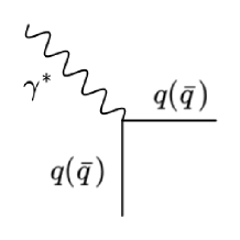
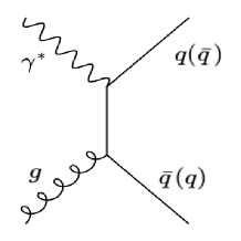
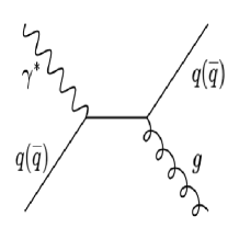
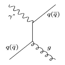
Figure 1: The panels from left to right shows the sub-processes, $\gamma^{\ast}+q\to q$ (Born level), $\gamma^{\ast}+g\to q+\bar{q}$ (boson-gluon), $\gamma^{\ast}+q\to q+g$ (Compton) and $\gamma^{\ast}+q\to q+g$ (Compton).

In the figure 2, the $(z,k_{t})$-factorization prescription is schematically shown with respect to its the corresponding partonic cross section $\hat{\sigma}(x,z,k_{t}^{2},\mu^{2})$. In this framework a parton with momentum $k_{n-1}$ that evolves according to the DGLAP evolution equation, with the factorization scale $k_{t}$, is emitted a parton with momentum $k^{\prime}_{n}=k_{n-1}-k_{n}$ and becomes $k_{n}$, and enters into the hard interaction with the virtual photon, which has virtuality $Q^{2}$, where $q^{2}=-Q^{2}$. It can be shown that Watt et al. (2003), these diagrams with quark (gluon) that comes into hard interaction (as can be seen in the upper panel (lower panel) of the figure 2), can actually in the leading logarithmic approximation be factorized into the DUPDFs and the hard scattering process that now depends to additional fractional momentum $z$, i.e., $\hat{\sigma}^{\gamma^{*}{q(g)}}(x,z,k_{t}^{2},\mu^{2})$. In this work, we only consider the Born level sub-process, see the left panel of the figure 1, where the incoming parton has the momentum $k_{n}$, which is actually a dijet process in the leading logarithm approximation as we said before. One of these jets, i.e., current jet, has the momentum $k_{n}+q$ and the other one which is emitted in the last step has the momentum $k_{n}^{\prime}$. Using the Sudakov decomposition, the four-vector $k_{n}$ can be described in terms of two light-like vectors $P$, the momentum of proton, and $q^{\prime}\equiv q+x_{B}P$, in addition to the space-like transverse momentum, $k_{T}$, where the following relations are hold:

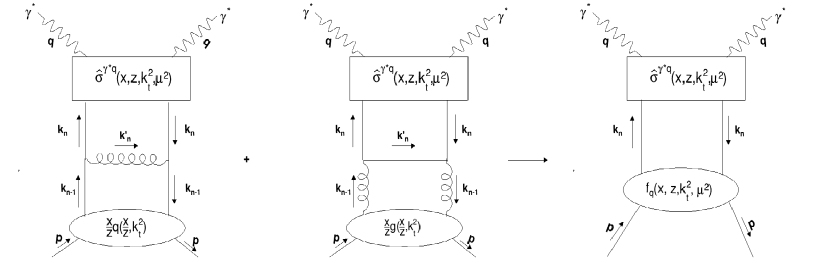
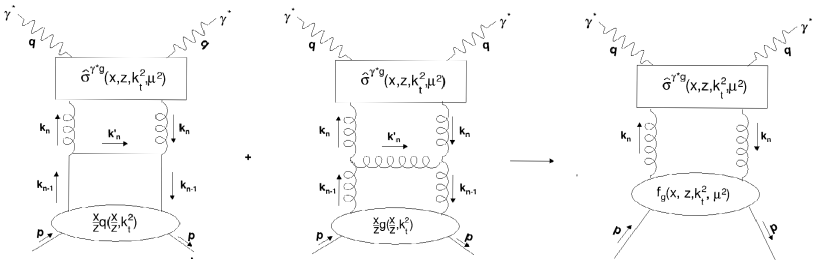
Figure 2: The pictorial representation of the $(z,k_{t})$-factorization for the quark DUPDF (the three diagrams in the upper panel) and the gluon DUPDF (the three diagrams in the lower panel). The first two diagrams in the upper and lower panels show a collinear parton with four-momentum $k_{n-1}$ that emits a parton and its four-momentum becomes $k_{n}$ Watt et al. (2003).

$$P^{2}=q^{{\prime}2}=P.k_{T}=q^{\prime}.k_{T}=0$$ (35)

$$k_{T}^{2}=-k_{t}^{2},\;\;\;\;\;P.q^{\prime}=\dfrac{Q^{2}}{2x_{Bj}}$$ (36)

Therefore the momenta of $k_{n}$ and $k_{n-1}$ can be written as follows:

$$k_{n}=xP-\beta q^{\prime}+k_{T},$$ (37)

$$k_{n-1}=\dfrac{x}{z}P.$$ (38)

One can obtain $\beta$ from the equation 37, using the on-shell condition of the emitted parton in the last step of evolution chain, i.e.,:

$${k_{n}^{\prime}}^{2}=(k_{n-1}-k_{n})^{2}=0\implies\beta=\dfrac{zk_{t}^{2}x_{Bj}}{x(1-z)Q^{2}}.$$ (39)

Here, the full kinematic of the parton in the last step of the evolution is taken into account, and one can see that $k_{n}^{2}=k_{t}^{2}/(1-z)$, in contrast to the $k_{t}$-factorization framework, where $z\to 0$ and as a result of this, one obtains $k=xP+k_{t}$, and $k^{2}=-k_{t}^{2}$. Additionally, using the constraint $(k_{n}+q)^{2}=0$, one can obtain the following relation for $x$:

$$x_{\pm}=\dfrac{x_{Bj}}{2(1-z)}\left(1-z+\frac{k_{t}^{2}}{Q^{2}}\pm\sqrt{{(1-z+\frac{k_{t}^{2}}{Q^{2}})}^{2}-4\frac{k_{t}^{2}}{Q^{2}}z(1-z)}\right).$$ (40)

In order to calculate the cross section one need to use the momenta of partons in the Briet frame. In this frame, the virtual photon only has component of momentum along the $z$ direction $q=(0,0,0,-Q)$. Then if we use the above equations 35 and 36, and utilize the light-cone components, the momenta can be written as follows:

$$p=\dfrac{1}{\sqrt{2}}(Q/x_{Bj},0,\boldsymbol{0}),\;\;\;\;\;q^{\prime}=\dfrac{1}{\sqrt{2}}(0,Q,\boldsymbol{0}),\;\;\;\;\;k_{T}=(0,0,\boldsymbol{k_{t}}),$$ (41)

where we use the definition of $a=(a^{+},a^{-},a_{T})$, with $a^{+}=(a_{0}+a_{3})/\sqrt{2}$ and $a^{-}=(a_{0}-a_{3})/\sqrt{2}$ for the light-cone variables Collins (1997). Now, these momenta can be used to obtain the following rapidities for the current jet:

$$\eta^{Breit}=\dfrac{1}{2}\ln{\dfrac{k_{n}^{+}+q^{+}}{k_{n}^{-}+q^{-}}}=\dfrac{1}{2}\log{\dfrac{x/x_{B}-1}{1-\beta}},$$ (42)

and the last step emitted jet:

$$\eta^{Breit}=\dfrac{1}{2}\ln{\dfrac{k_{n-1}^{+}-k_{n}^{+}}{k_{n-1}^{-}-k_{n}^{-}}}=\dfrac{1}{2}\log{\dfrac{x(1-z)}{x_{B}z\beta}}.$$ (43)

To calculate the hadronic cross section, first, one needs to obtain the partonic cross section Watt et al. (2003), i.e.,

$$d\hat{\sigma}^{\gamma^{\ast}q^{\ast}}_{T,L}=d\Phi^{\gamma^{\ast}q^{\ast}}|M^{\gamma^{\ast}q^{\ast}}_{T,L}|^{2}/F^{\gamma^{\ast}q^{\ast}},$$ (44)

where $T$ and $L$ are denoted for the longitudinal and transverse virtual photon polarizations cross section. The flux factor and the phase space can be obtained as:

$$F^{\gamma^{\ast}q^{\ast}}=4xp.q=2xQ^{2}/x_{Bj},$$ (45)

$$d\Phi^{\gamma^{\ast}q^{\ast}}=2\pi\dfrac{x_{Bj}}{Q^{2}}\sum_{i=\pm}\dfrac{1}{(1-x_{Bj}\beta/x)}\delta(x-x_{i}),$$ (46)

respectively, where $x_{i}$ is defined in the equation 40, and because $x_{Bj}\leq x$, it constraints $x$ to $x_{+}$.

The squared matrix elements in the equation 44 are given as follows:

$$|M_{T}^{\gamma^{\ast}q^{\ast}}|^{2}=4\pi\alpha_{em}e_{q}^{2}Q^{2}\dfrac{x}{x_{Bj}},\;\;\;\;\;\;\;\;\;\;\;\;\;\;|M_{L}^{\gamma^{\ast}q^{\ast}}|^{2}=0,$$ (47)

Now one can insert above different elements into equation 44 to get the partonic cross sections as:

$$\hat{\sigma}_{T}^{\gamma^{*}q^{\ast}}(x,z,k_{t}^{2},\mu^{2})=\frac{4\pi^{2}\alpha_{em}}{Q^{2}}e_{q}^{2}\dfrac{x_{B}}{1-x_{B}{\beta/x}}\delta(x-x_{+})\;\;\;with\;\;\;\hat{\sigma}_{L}^{\gamma^{*}q^{\ast}}(x,z,k_{t}^{2},\mu^{2})=0.$$ (48)

After using the above cross section in the equation 22, the hadronic cross section can be obtained, i.e,:

$$\sigma_{T}^{\gamma^{*}p}=\frac{4\pi^{2}\alpha}{Q^{2}}\int_{x}^{1}\;dz\;\int_{0}^{\infty}\frac{\mathrm{d}k_{t}^{2}}{k_{t}^{2}}\dfrac{{x_{B}}/x}{1-x_{B}{\beta/x}}\sum_{q}\;e_{q}^{2}f_{q}(x,z,k_{t}^{2},\mu^{2}).$$ (49)

Finally, using the above equation, the calculation of inclusive jet and dijet production in the electron-proton collision can be evaluated as:

$$\begin{split}\sigma(jet)=\int_{y_{min}}^{y_{max}}\;dy\;\int_{Q^{2}_{min}}^{Q^{2}_{max}}\;dQ^{2}\dfrac{\alpha}{2\pi yQ^{2}}[(1+(1-y)^{2}\sigma_{T}^{\gamma^{*}p}+2(1-y)\sigma_{L}^{\gamma^{*}p}]\\ \sum_{jets}\;\Theta(E_{T}-E_{T_{min}})\;\Theta(E_{T_{max}}-E_{T})\;\Theta(\eta-\eta_{min})\;\Theta(\eta_{max}-\eta),\end{split}$$ (50)

where $y$, $Q^{2}$, $E_{T}$, $\eta$ are the inelasticity, the virtuality, the transverse energy of produced jets, and the pseudo-rapidity, respectively. Then we can calculate the above differential cross section Watt et al. (2003), as:

$$d\sigma/dO=\sigma(jet)/(O_{max}-O_{min}),$$ (51)

where $O$ can be any physical observable such as $E_{T}$, $M_{jj}$ etc.. Also the denominator in the above formula is the size of each bin.

III.3 The numerical methods for the differential cross sections calculation of high $Q^{2}$ in the inclusive jet and dijet

In contrast to the calculation of $k_{t}$-factorization framework of the section II, which was done by the KaTie event generator, we directly calculate the high $Q^{2}$ inclusive jet and dijet cross sections to be compared with those of ZEUS collaboration Abramowicz et al. (2010); et al. [ZEUS Collaboration] (2002). For the numerical calculation of these differential cross sections, we need to generate the DUPDFs for the three aforementioned models, see the sub-section III.1, and we should also use a method to numerically compute the multidimensional integral over $z$, $k_{t}^{2}$, $y$ and $Q^{2}$. The DUPDFs integrals are again calculated with the help of Gauss-Legendre quadrature method of the BOOST libraries. While the input PDFs for the DUPDFs, the central PDFs of MMHT2014lo68cl LHAPDF library are used. To perform the multidimensional integrals of the differential cross sections we resort to the VEGAS Monte-Carlo algorithm Press et al. (2007), with the limit of integrals over $y$ and $Q^{2}$ and also the cuts over $\eta$ and $E_{T}$ are set in accordance with the ZEUS collaboration data et al. [ZEUS Collaboration] (2002); Abramowicz et al. (2010). The factorization scale $\mu$ is set as Watt et al. (2004):

$$\mu=Q\dfrac{x}{x_{B}}\sqrt{\frac{1-\beta}{x/x_{B}-1}}.$$

As we mentioned in the section II.2, we again only include the first five quark flavors and their anti-quarks in our calculation. Here an important point about the Born level process, in which the jets are widely separated from each other, is that there is a one to one relation between the momentum of partons and jets, and hence using the jet algorithm for calculation of the inclusive jet and the dijet at this level of perturbation theory is unnecessary Watt et al. (2003).

IV Numerical results and discussions

In this section, our predictions of the different differential cross sections for the inclusive jet and dijet cross sections, using the $k_{t}$ and $(z,k_{t})\textrm{-factorizations}$ are compared to the experimental data of ZEUS collaboration et al. [ZEUS Collaboration] (2002); Abramowicz et al. (2010). In the inclusive jet experiment et al. [ZEUS Collaboration] (2002), positrons of energy $27.5\;GeV$ are collided with the protons of energy $820\;GeV$. While for the inclusive dijet experiment Abramowicz et al. (2010), the electrons or the positrons of energy $27.5\;GeV$ are collided with the protons of energy $920\;GeV$. The inelasticity in the inclusive dijet experiment is between $0.2$ and $0.6$, while in the inclusive jet experiment it is fixed by $-0.7<\cos{\gamma}<0.5$, where $\cos{\gamma}$ is defined as:

$$\cos\gamma=\dfrac{x_{B}(1-y)E_{p}-yE_{e}}{x_{B}(1-y)E_{p}+yE_{e}}.$$ (52)

The virtuality $Q^{2}$ for both experiments is larger than $125\;GeV^{2}$, but for the dijet experiment is limited to $Q^{2}<20000\;GeV^{2}$. For the inclusive jet experiment at least one jet has the transverse energy in the Breit frame larger than $8\;GeV$ and $-2<\eta^{jet}_{B}<1.8$, and for the inclusive dijet experiment the highest transverse energies of the two jets should be larger than $8\;GeV$, with $-1<\eta_{Lab}^{jet}<2.5$. In addition to these limits, there is also one additional constraint on the invariant mass of the final dijet state, which limits the dijet invariant mass to $M_{jj}>20\;GeV$. The tested channels of differential cross sections that we consider here are as following:

• The inclusive jet cross sections:

  1. $\dfrac{d\sigma}{dE_{T,B}^{jet}}$: The differential cross section with respect to the transverse energies of the final state jets in the Breit Frame.

  2. $\dfrac{d\sigma}{d\eta_{B}^{jet.}}$: The differential cross section with respect to the pseudo-rapidity of the final state jets in the Breit Frame.

  3. $\dfrac{d\sigma}{dQ^{2}}$: The differential cross section with respect to the virtuality.

• The inclusive dijet cross sections:

  1. $\dfrac{d\sigma}{d\overline{E_{T,B}^{jet}}}$: The differential cross section with respect to the mean transverse jet energy in the Breit frame

  2. $\dfrac{d\sigma}{dQ^{2}}$: The differential cross section with respect to the virtuality.

  3. $\dfrac{d\sigma}{d\eta^{\ast}}$: The differential cross section with respect to the half difference of the jet pseudo-rapidities in the Breit frame, where $\eta^{\ast}$ is defined as $|\eta_{B}^{jet1}-\eta_{B}^{jet2}|/2$.

  4. $\dfrac{d\sigma}{dM_{jj}}$: The differential cross section with respect to the invariant mass of dijet.

Before discussing our results, we first give an overview of different DGLAP based UPDFs and DUPDFs that we use in this work as follows (these abbreviations are also used to show the related differential cross sections in the figures 4 to 14):

• UPDFs:

  1. KMR: This formalism assumes that the parton evolves up to the last evolution step according to the DGLAP evolution equation, but in this step it gains transverse momentum and does not radiate any real emissions further more. Therefore no real emission to the factorization scale is re-summed by the Sudakov form factor. In this method, the soft gluon emission singularity is cured by using the angular ordering of the soft gluon, the quark and anti-quark, emissions (see the subsection II.1.1).

  2. LO-MRW: This formalism is the same as the KMR, but without additional angular ordering constraint on the quark (anti-quark) emissions (see the subsection II.1.2) .

  3. NLO-MRW: This formalism is the same as the LO-MRW, but with the virtuality $k^{2}=\dfrac{k_{t}^{2}}{(1-z)}$ for the scale in the DGLAP evolution equation, and the strong ordering cutoff $\Theta(\mu^{2}-k^{2})$ on the virtuality. For curing the divergency due to the soft gluon emission, the angular ordering of soft gluon emissions is imposed. Additionally, the NLO level PDFs and the splitting functions are used (see the subsection II.1.2).

• DUPDFs:

  1. DKMR: This formalism is the same as the KMR, but the integral over z is not performed (see the subsection III.1.1).

  2. DMRW: This formalism is the same as the LO-MRW, but the integral over z is not performed (see the subsection III.1.2).

  3. DMRW^′: This formalism is the same as DMRW, but with $k_{t}$ replaced by $k$ and also adding a $\Theta(\mu^{2}-k^{2})$ to prevent $k^{2}$ becomes larger than $\mu^{2}$ (see the subsection III.1.2).

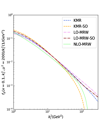
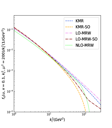
Figure 3: The left and right panels show the comparison of the up quark and gluon UPDFs/$k_{t}^{2}$ of the KMR, LO-MRW and NLO-MRW (KMR-SO and LO-MRW-SO) with the angular (strong ordering) cutoff, respectively. See the text for more explanations.

For example, in order to gain an insight about the behavior of our different UPDFs, in the figure 3 we have plotted the KMR, LO-MRW and NLO-MRW UPDFs/$k_{t}^{2}$ for the gluon and the up quark at x=0.1 and $\mu^{2}=200$ $GeV^{2}$. The KMR-SO and LO-MRW-SO are the corresponding UPDFs/$k_{t}^{2}$, but using the strong ordering constraint. As it was discussed in the references Hosseinkhani and Modarres (2011, 2012), the results of different UPDFs models with the angular ordering constraint are very similar, especially at small transverse momentum. In case of strong ordering (KMR-SO), the UPDFs go to zero for $k_{t}^{2}\sim\mu^{2}$. On the other hand in the case of MRW-SO, since the constraint is only imposed on the gluon emission terms, the corresponding distribution becomes different from the KMR-SO. We will come back to the effect of above UPDFs on the differential cross sections later on.

In what follows we discuss and elaborate upon the differential cross-section predictions using different UPDFs, i.e., KMR, LO-MRW and NLO-MRW and DUPDFs, i.e., DKMR, DMRW and DMRW^′, in the $k_{t}$ and $(z,k_{t})\textrm{-factorization}s$ models, by comparing their results to the data and to each other, see the figures 4 to 14. In all of these figures, it is observed that the LO-MRW and DMRW differential cross sections are larger with respect to the other models presented in these figures. On the other hand the corresponding KMR and LO-MRW, and DKMR and DMRW differential cross sections are close to each other. As we pointed out before, these similarities can be due to the UPDFs of the KMR and LO-MRW which is demonstrated at $x=0.1$ and $\mu^{2}=200$ in the figure 3.

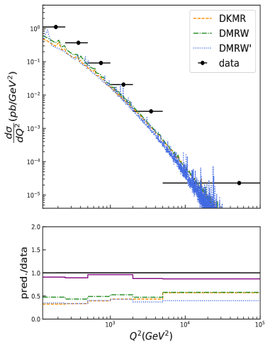
Figure 4: The left and right panels show the comparison of inclusive jet production cross sections, ($d\sigma/dQ^{2}$), for the $(z,k_{t})$-factorization with the DUPDFs models, i.e., DKMR, DMRW, and DMRW^′, and the $k_{t}$-factorization with the UPDFs models, i.e., KMR, LO-MRW, and the NLO-MRW with respect to the experimental data et al. [ZEUS Collaboration] (2002). The below panels demonstrate predictions ratio of our models and the NLO collinear (solid-purple line) to the data et al. [ZEUS Collaboration] (2002), respectively.

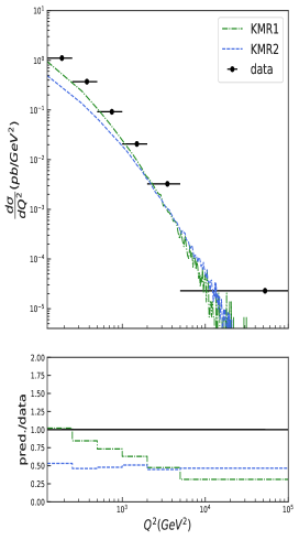
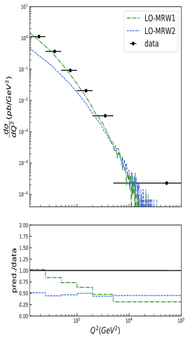
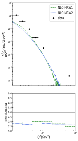
Figure 5: The contribution of each sub-processes to inclusive jet differential cross section, $d\sigma/dQ^{2}$, with respect to the experimental data et al. [ZEUS Collaboration] (2002) for the KMR, LO-MRW and the NLO-MRW, i.e., $\gamma^{\ast}+q\to q$ (Born level) (KMR1, LO-MRW1, NLO-MRW1) and $\gamma^{\ast}+q\to q+g$ (boson-gluon), $\gamma^{\ast}+g\to q+\bar{q}$ (Compton) and $\gamma^{\ast}+g\to q+\bar{q}$ (Compton) (KMR2, LO-MRW2, NLO-MRW2). See the figure 1.

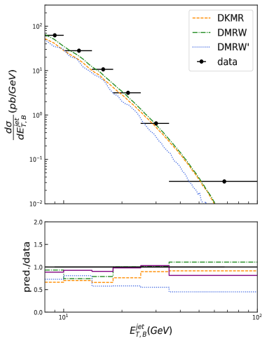
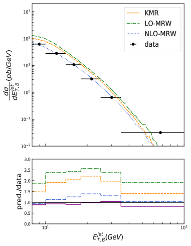
Figure 6: The same as the figure $4$ but for $d\sigma/dE_{T,B}^{jet}$.

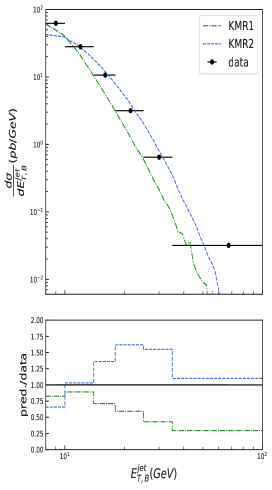
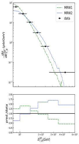
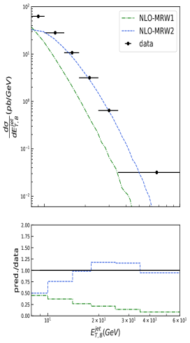
Figure 7: The same as the figure $5$ but for $d\sigma/dE_{T,B}^{jet}$.

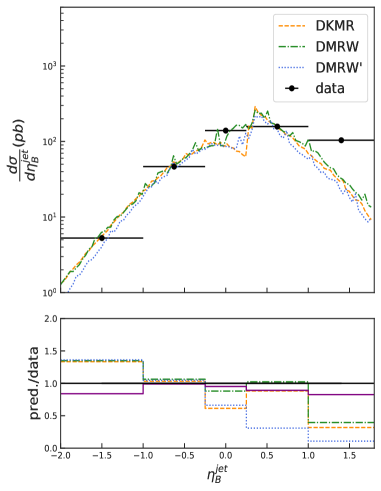
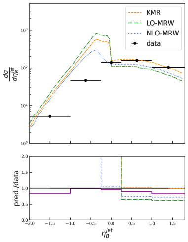
Figure 8: The same as figure $4$ but for $d\sigma/d\eta^{jet}_{Breit}$.

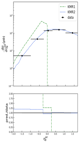
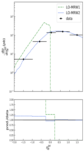
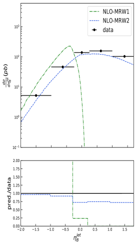
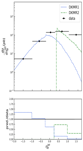
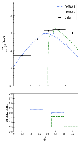
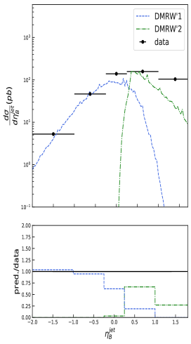
Figure 9: The top panel is the same as the figure $5$ but for $d\sigma/d\eta^{jet}_{Breit}$. The bottom panel is $d\sigma/d\eta^{jet}_{Breit}$ but for the current (DKMR1, DMRW1, and DMRW^′1) and the last step (DKMR2, DMRW2, and DMRW^′2) emitted jets for different DUPDFs models .

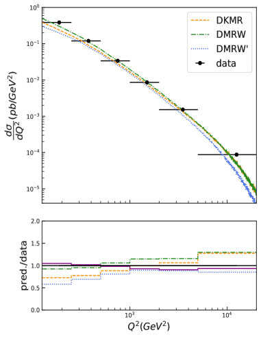
Figure 10: The same as the figure 4 but for the inclusive dijet production. The experimental data and the NNLO collinear result are from the references Abramowicz et al. (2010) and Currie et al. (2017), respectively.

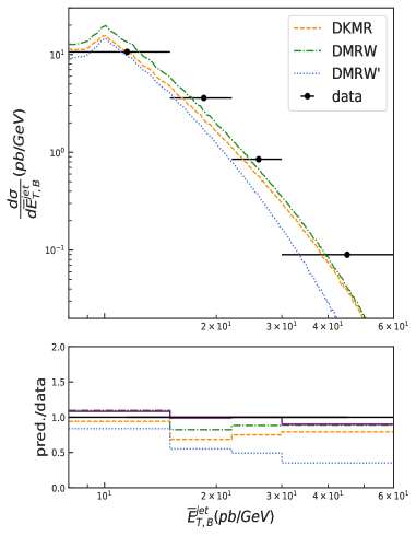
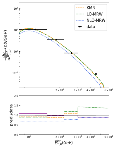
Figure 11: The same as the figure $10$ but for $d\sigma/d\overline{E}_{T,B}^{jet}$.

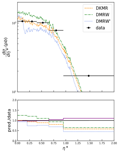
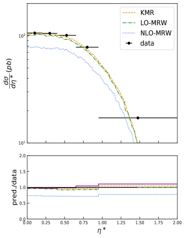
Figure 12: The same as the figure $10$ but for $d\sigma/d\eta^{\ast}$.

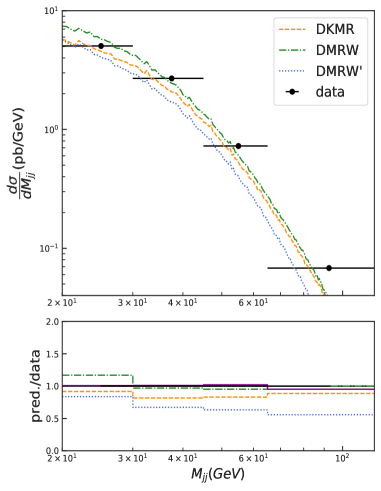
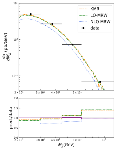
Figure 13: The same as the figure $10$ but for $d\sigma/dM_{jj}$.

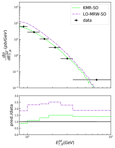
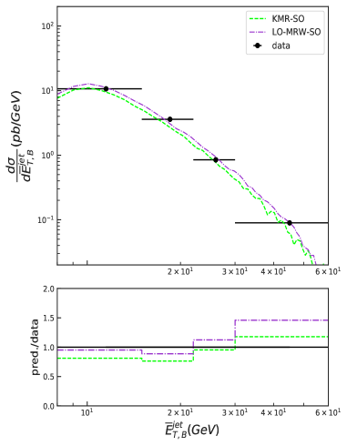
Figure 14: The same as the figure $6$ ($10$), left (right) panel, but for the KMR and LO-MRW strong ordering constraint.

The same similarity is also expected for the corresponding differential cross sections with input DUPDFs, because only the difference between the DUPDFs and the UPDFs are the integration over $z$ which is not performed in the DUPDFs cases.

Another important feature that is demonstrated in the figure 3 is the smaller distribution of up quark and gluon of the NLO-MRW with respect to the other UPDFs except that of KMR-SO. Actually, this choice of virtuality for the scale, i.e., $k^{2}=\dfrac{k_{t}^{2}}{(1-z)}$, leads to the larger argument of the PDFs with respect to the KMR and LO-MRW UPDFs. Because we are working in the region that the larger fractional momenta play the significant role. Therefore the strong ordering cutoff, $\Theta(\mu^{2}-k^{2})$, on the virtuality in the NLO-MRW UPDF and the DMRW^′ is a crucial factor in the sharp decrease of these UPDFs and DUPDFs at this energy scales. These behaviors also show themselves directly in the differential cross section calculations.

Additionally, by looking at the bottom panels of each plot, i.e., the figures 4 to 13, one finds that the results of the NLO et al. [ZEUS Collaboration] (2002) and NNLO Currie et al. (2017) of the collinear factorizations (denoted by solid-purple color) have better agreement to the data with respect to our calculation. However, as it was discussed in the reference Watt et al. (2004), we should point out that, the result of present calculation should not be as good as collinear approaches, on the other hand, it is more simplistic, considering the computer time consuming, i.e., the fewer number of tree-level Feynman diagrams are needed for calculation in the $k_{t}$-factorization framework with respect to the collinear one for calculation of the corresponding differential cross sections. Hence such feature makes the $k_{t}$-factorization computationally more efficient (in order to see more the details on how higher order diagrams are included in the tree level lower order diagrams in the $k_{t}$-factorization formalisms, one can see the section $3$ of the reference Andersson et al. (2002)). Despite the fact that this framework is more convenient than the collinear factorization approach, however the complications which arise by including the transverse momentum of the evolving parton into calculation, and obtaining an evolution equation, that can perfectly work in all kinematic regimes, becomes a hard task. For example the Catani–Ciafaloni-Fiorani–Marchesini (CCFM) evolution equation Ciafaloni (1988); Catani et al. (1990a, b); Marchesini (1995) which is one of the successful evolution equations, has the limitation that cannot give transverse momentum densities for all quark flavors and is limited to the valence flavors of up and down quarks. Therefore, testing different UPDFs models and obtaining a suitable approach to create the UPDFs have significant importance in the current field of high energy.

In the figures 4 to 9, we compare predictions of the differential cross sections in the $k_{t}$ and $(z,k_{t})$-factorizations with the data only for the inclusive jet production. It is observed that the KMR and LO-MRW predictions of differential cross sections overshoot the data in the figures 6 and 8. The main factor for such a behavior is linked to the large contribution of the Born level subprocess, see figures 5, 7 and 9 in which the Born level and dijet sub-processes plotted separately. We should note here that the Born level subprocess, is not included in the collinear factorization calculation. In fact, in the Breit frame, within the collinear factorization approach et al. [ZEUS Collaboration] (2002), the parton that comes into the hard interaction has only the component of momentum along the direction of proton, i.e., $\hat{z}$. Therefore, the parton struck with the virtual photon which has also a component along the $-\hat{z}$ direction, and it scattered back with zero transverse momentum. The contribution of such process in the collinear-factorization approach is completely suppressed due to the experimental cut on $E_{T,B}^{jet}$.

It can be visualized from the figures 4 and 6, i.e. $d\sigma/dQ^{2}$ and $d\sigma/dE_{T,B}^{jet}$, that the results of the NLO-MRW are relatively good, while it gets worse for $\eta_{B}^{jet}<0$, in $d\sigma/d\eta_{B}^{jet}$, due to the large contribution of the Born level sub-process.

The contribution of Born level and dijet sub-processes (see the sub-processes given in the figure 1) are separately shown in the figures 7 and 9. It is shown that the results of dijet contributions with the KMR and MRW UPDFs can only give relatively more satisfactory results with respect to the Born-level sub-process. So the overshoot of the data in the $k_{t}$-factorization approach, presented in the figure 6, may not be connected with the double counting of the last step emission. Because in our event generation, we impose a cutoff on the transverse momentum of the incoming parton of the Born level sub-process to be less than the factorization scale, and also additional cutoff is set, which limits the transverse momentum of the incoming parton to be less than the minimum of hard jets transverse momenta. This procedure is similar to the method given in the reference Maciula and Szczurek (2019), which suppresses the hard last step emitted jets and double counting which may happen.

In contrast to the results of the $k_{t}$-factorization which overshoots the data, the predictions of the DKMR and DMRW DUPDFs of the $(z,k_{t})$-factorization are in relatively good agreement with the data of $d\sigma/d\eta_{B}^{jet}$ and $d\sigma/dE_{T,B}^{jet}$ channels of the inclusive jet predictions. However these predictions undershoot the data of $d\sigma/dQ^{2}$. We also see the results of the DMRW^′ underestimates the data due to the reasons explained before.

One interesting point about the results of the $(z,k_{t})$-factorization framework is that the predicted differential cross section have a similar behavior with respect to the dijet in the $k_{t}$-factorization method, in which one can observe that their results are in good agreement to the data, except the channel of $d\sigma/dQ^{2}$. In other words, we can obtain similar results to the dijet sub-processes in the $k_{t}$-factorization formalism, but just with the inclusion of the Born level diagram.

In addition to the above points, there can be seen a non-smooth behavior in the $\eta_{B}^{jet}\approx 0$ of $d\sigma/d\eta_{B}^{jet}$ channel. This behavior in case of the $(z,k_{t})$-factorization differential cross section is due to the involvement of the last step emission in the region $\eta_{B}^{jet}>0$, i.e. there is no contribution of the last step emission in $\eta_{B}^{jet}<0$ region (see the predictions of different DUPDFs models in the bottom panel of the figure 9). However this non-smooth behavior in the results of UPDF models of the $k_{t}$-factorization framework (as can be seen in the top panel of the figure 9) is due to this fact that the Born level process only contributes in the $\eta_{B}^{jet}<0$.

The inclusive dijet differential cross section calculations in the $k_{t}$ and $(z,k_{t})$-factorization approaches are illustrated in the figures 10-13. One can observe that the UPDF models of the KMR and LO-MRW, and their corresponding DUPDFs are quiet successful in describing the data. However the results of NLO-MRW and DMRW^′, due to the reasons mentioned before, underestimate the data. It should be noted that some of our results are even comparable with the NNLO collinear predictions, even though only the tree level diagrams of $\gamma^{\ast}+q\to q+g$ and $\gamma^{\ast}+g\to q+\bar{q}$ processes are calculated within the $k_{t}$-factorization framework. We should also again repeat here that in the calculation of inclusive dijet production in the $(z,k_{t})$-factorization, we only include the Born level sub-process $\gamma^{\ast}+q\to q$, while in this framework, the $\gamma^{\ast}+q\to q+g$ and $\gamma^{\ast}+g\to q+\bar{q}$ sub-processes are actually three jets processes, where the last step emission is also directly comes into play in contrast to the $k_{t}$-factorization formalism. Therefore we neglected these sub-processes in our numerical calculation of $(z,k_{t})$-factorization framework.

It is also interesting to present the results of $k_{t}$ and $(z,k_{t})$-factorizations for the data of $\dfrac{d\sigma}{dQ^{2}}$ in the figure 10. In contrast to the same data of inclusive jet production, the figure 4, it is observe that the results of the dijet sub-processes, using the UPDFs of KMR and MRW, and also their corresponding DUPDFs have excellent agreement with the data.

Finally, considering the comparison of the results differential cross section calculation with LO-MRW UPDF using the angular and strong ordering constraints, one can clearly conclude that considereing the inclusive dijet data, the predictions of LO-MRW UPDFs with angular constraint does not have large discrepancy with the data. On the other hand the prediction of the LO-MRW with strong ordering cutoff is similar to the LO-MRW with angular ordering constraint. On the other hand, the prediction of the KMR with strong ordering constraint is clearly much smaller than the KMR with angular ordering cutoff. This is mostly due to additional cutoff on the non-diagonal term of the DGLAP evolution equation of the unintegrated gluon distribution function, i.e. the second term of the equation 10. Because in this range of energy, the quark contents of the proton have the dominant distributions, then such an additional cutoff can lead to smaller prediction of these UPDFs at this range of energy. Additionally, in the case of the inclusive jet production, the LO-MRW with the strong ordering cutoff does not have huge effect to the results of the inclusive jet production, and its result (as can be seen in the left panel of figure 14) still overshoot the data. While the result of the KMR with strong ordering cutoff, although becomes closer, but still overshoot the data. Therefore, as can be seen from the figure 14 using the strong ordering cutoff does not necessarily improves the predictions of the KMR and LO-MRW models, and also the predictions of the KMR and LO-MRW models do not overshoot the data significantly as suggested in the references Guiot (2019, 2020).

V Conclusions

We calculated the inclusive jet and dijet cross sections in the $k_{t}$ and $(z,k_{t})\textrm{-factorizations}$ formalisms. For calculation of the differential cross sections in the $k_{t}\textrm{-factorization}$ model , we used the KaTie event generator with the $\gamma^{\ast}+q\to q+g$ and $\gamma^{\ast}+g\to q+\bar{q}$ sub-processes, as well as $\gamma^{\ast}+q\to q$ for the inclusive jet production, by considering different UPDF approaches, i.e., the KMR, LO-MRW and NLO-MRW. While for the $(z,k_{t})\textrm{-factorization}$ approach we directly calculated the $\gamma^{\ast}+q\to q$, and we also used the DUPDFs analogous to the aforementioned UPDFs in the $k_{t}\textrm{-factorization}$ framework.

We observed that, in general, the differential cross sections using the NLO-MRW UPDF underestimates the data due to the choice of virtuality as the factorization scale of the DGLAP evolution equation, in addition to the strong ordering cutoff on virtuality with the hard cutoff $\Theta(\mu^{2}-k^{2})$. It was observed that the UPDFs of the KMR and LO-MRW formalisms show the same behavior in this range of the center of mass energy, and the $k_{t}$-factorization is inadequate in describing the data of inclusive jet production due to the large role of the Born level sub-process, i.e. $\gamma^{\ast}+q\to q$. While the same Born level sub-process in the $(z,k_{t})$-factorization was actually the dijet processes in the leading logarithmic approximation and gave adequate results for all channels but not for $d\sigma/dQ^{2}$.

In order to investigate the predictions made in the references Guiot (2019, 2020), we also calculated $d\sigma/dE_{T,B}^{jet}$ and $d\sigma/d\overline{E}_{T,B}^{jet}$ of the inclusive jet and dijet cross sections with the LO-MRW and KMR UPDFs, in which the strong ordering of the gluon emissions was used for curing soft gluon divergency. We found that this cutoff in the inclusive dijet cross section makes no significant effect on the prediction of the LO-MRW formalism, but the result of KMR with this cutoff falls much more below the angular ordering prediction. However, in case of the experimental data of inclusive jet production, even with the strong ordering cutoff still the predictions of the KMR and LO-MRW with strong ordering constraint overshoot the data. Therefore we found that using the strong ordering cutoff does not necessary improves the predictions of the KMR and LO-MRW at these range of energies.

It was also found out that the $k_{t}$-factorization can in fact be a suitable framework for describing the data of inclusive dijet production. Even some of its results were comparable with the NNLO collinear factorization framework calculations.

Finally, we observed that due to including the last step emission into our calculation, the $(z,k_{t})$-factorization can describe the data of inclusive jet and dijet cross sections relatively good, and can be a suitable alternative for the $k_{t}$-factorization framework.

References

- Collins et al. (1988) J. C. Collins, D. E. Soper, and G. Sterman, Adv. Ser. Direct. High Energy Phys. 5, 1 (1988).
- Collins (2011) J. Collins, Foundations of Perturbative QCD (Cambridge University Press, Cambridge, 2011).
- Catani et al. (1991) S. Catani, M. Ciafaloni, and F. Hautmann, Nucl. Phys. B 366, 135 (1991).
- Collins and Ellis (1991) J. C. Collins and R. K. Ellis, Nucl. Phys. B 360, 3 (1991).
- Andersson et al. (2002) B. Andersson et al., Eur. Phys. J. C 25, 77 (2002).
- Andersson et al. (2004) B. Andersson et al., Eur. Phys. J. C 35, 67 (2004).
- Andersen et al. (2006) B. Andersson et al., Eur. Phys. J. C 48, 53 (2006).
- Watt et al. (2003) G. Watt, A. D. Martin, and M. G. Ryskin, Eur. Phys. J. C 31, 73 (2003).
- Niehues and Walker (2019) J. Niehues and D. M. Walker, Phys. Lett. B 788, 243 (2019).
- Catani et al. (2012) Catani et al., Phys. Rev. Lett. 108, 072001 (2012).
- Boughezal et al. (2015a) R. Boughezal, C. Focke, et al., Phys. Rev. Lett. 115, 062002 (2015a).
- Gehrmann et al. (2014) T. Gehrmann et al., Phys. Rev. Lett. 113, 212001 (2014).
- Czakon et al. (2013) M. Czakon, P. Fiedler, and A. Mitov, Phys. Rev. Lett. 110, 252004 (2013).
- Currie et al. (2018) J. Currie, T. Gehrmann, E. Glover, A. Huss, J. Niehues, and A. Vogt, JHEP 2018, 209 (2018).
- Cieri et al. (2019) L. Cieri, X. Chen, T. Gehrmann, E. Glover, and A. Huss, JHEP 2019, 96 (2019).
- Freitas (2016) A. Freitas, Prog. Part. Nucl. Phys. 90, 201 (2016).
- Boughezal et al. (2015b) R. Boughezal, X. Liu, and F. Petriello, Phys. Rev. D 91, 094035 (2015b).
- Catani and Grazzini (2007) S. Catani and M. Grazzini, Phys. Rev. Lett. 98, 222002 (2007).
- Cacciari et al. (2015) M. Cacciari, F. A. Dreyer, A. Karlberg, G. P. Salam, and G. Zanderighi, Phys. Rev. Lett 115, 082002 (2015).
- Kimber et al. (2001) M. A. Kimber, A. D. Martin, and M. G. Ryskin, Phys. Rev. D 63, 114027 (2001).
- Martin et al. (2010) A. D. Martin, M. G. Ryskin, and G. Watt, Eur. Phys. J. C 66, 163 (2010).
- Modarres and Hosseinkhani (2009) M. Modarres and H. Hosseinkhani, Nucl.Phys.A 815, 40 (2009).
- Modarres and Hosseinkhani (2010) M. Modarres and H. Hosseinkhani, Few-Body Syst. 47, 237 (2010).
- Hosseinkhani and Modarres (2011) H. Hosseinkhani and M. Modarres, Phys.Lett.B 694, 355 (2011).
- Hosseinkhani and Modarres (2012) H. Hosseinkhani and M. Modarres, Phys.Lett.B 708, 75 (2012).
- Modarres et al. (2013) M. Modarres, H. Hosseinkhani, and N. Olanj, Nucl.Phys.A 902, 21 (2013).
- Modarres et al. (2014) M. Modarres, H. Hosseinkhani, and N. Olanj, Phys.Rev.D 89, 034015 (2014).
- Modarres et al. (2017a) M. Modarres, H. Hosseinkhani, and N. Olanj, Int.J.Mod.Phys.A 32, 1750121 (2017a).
- Modarres et al. (2015) M. Modarres, H. Hosseinkhani, N. Olanj, and M. Masouminia, Eur.Phys.J.C 75, 556 (2015).
- Modarres et al. (2016a) M. Modarres, M. Masouminia, H. Hosseinkhani, and N. Olanj, Nucl.Phys.A 945, 168 (2016a).
- Modarres et al. (2016b) M. Modarres, M. Masouminia, H. Hosseinkhani, and N. Olanj, Phys. Rev. D 94, 074035 (2016b).
- Modarres et al. (2016c) M. Modarres, M. Masouminia, R. Aminzadeh Nik, H. Hosseinkhani, and N. Olanj, Phys. Rev. D 94, 074035 (2016c).
- Modarres et al. (2017b) M. Modarres, M. Masouminia, R. Aminzadeh Nik, H. Hosseinkhani, and N. Olanj, Phys.Lett.B 772, 534 (2017b).
- Modarres et al. (2017c) M. Modarres, M. Masouminia, R. Aminzadeh Nik, H. Hosseinkhani, and N. Olanj, Nucl.Phys.B 922, 94 (2017c).
- Modarres et al. (2018) M. Modarres, M. Masouminia, R. Aminzadeh Nik, H. Hosseinkhani, and N. Olanj, Nucl. Phys. B 926, 406 (2018).
- Aminzadeh Nik et al. (2018) R. Aminzadeh Nik, M. Modarres, and M. R. Masouminia, Phys. Rev. D 97, 096012 (2018).
- Modarres et al. (2019) M. Modarres, R. Aminzadeh Nik, R. Kord Valeshbadi, H. Hosseinkhani, and N. Olanj, J. Phys. G 46, 105005 (2019).
- Lipatov and Malyshev (2016) A. V. Lipatov and M. A. Malyshev, Phys. Rev. D 94, 034020 (2016).
- Baranov et al. (2014) S. P. Baranov, A. V. Lipatov, and N. P. Zotov, Phys. Rev. D 89, 094025 (2014).
- Lipatov and Zotov (2014) A. V. Lipatov and N. P. Zotov, Phys. Rev. D 90, 094005 (2014).
- Watt et al. (2004) G. Watt, A. D. Martin, and M. G. Ryskin, Phys. Rev. D 70, 014012 (2004).
- Golec-Biernat and Staśto (2018) K. Golec-Biernat and A. M. Stasto, Phys. Lett. B 781, 633 (2018).
- Guiot (2019) B. Guiot, Phys. Rev. D 99, 074006 (2019).
- Guiot (2020) B. Guiot, Phys. Rev. D 101, 054006 (2020).
- Hautmann et al. (2018) F. Hautmann, H. Jung, A. Lelek, V. Radescu, and R. Zlebcik, JHEP 2018, 70 (2018).
- Hautmann et al. (2017) F. Hautmann, H. Jung, A. Lelek, V. Radescu, and R. Zlebcik, Phys. Lett. B 772, 446 (2017).
- Hautmann et al. (2019) F. Hautmann, L. Keersmaekers, A. Lelek, and A. van Kampen, Nucl. Phys. B 949, 114795 (2019).
- et al. [ZEUS Collaboration] (2002) S. Chekanov. et al. [ZEUS Collaboration], Physics Letters B 547, 164 (2002).
- Abramowicz et al. (2010) H. Abramowicz, I. Abt, Adamczyk, et al., Eur. Phys. J. C 70, 965 (2010).
- Currie et al. (2017) J. Currie, T. Gehrmann, A. Huss, et al., JHEP 2017, 209 (2017).
- van Hameren (2018) A. van Hameren, Comput. Phys. Commun. 224, 371 (2018).
- Kimber (2001) M. A. Kimber, Doctoral, Durham University (2001), URL http://etheses.dur.ac.uk/3848/.
- Gribov and Lipatov (1972) V. N. Gribov and L. N. Lipatov, Yad. Fiz. 15, 781 (1972).
- Altarelli and Parisi (1977) G. Altarelli and G. Parisi, Nucl. Phys. B 126, 298 (1977).
- Dokshitzer (1977) Y. L. Dokshitzer, Sov. Phys. JETP 46, 641 (1977).
- Marchesini and Webber (1984) G. Marchesini and B. Webber, Nucl. Phys. B 238, 1 (1984).
- Kimber et al. (2000) M. Kimber, A. Martin, and M. Ryskin, Eur. Phys. J. C 12, 655 (2000).
- (58) A. van Hameren, private communication(2021).
- Devenish and Cooper-Sarkar (2004) R. Devenish and A. Cooper-Sarkar, Deep inelastic scattering, Oxoford University Press (2004).
- Hautmann et al. (2014) F. Hautmann, Jung, et al., Eur. Phys. J. C 74 (2014).
- Harland-Lang et al. (2015) L. A. Harland-Lang, A. D. Martin, P. Motylinski, and R. S. Thorne, Eur. Phys. J. C 75, 435 (2015).
- Harland-Lang et al. (2016) L. A. Harland-Lang, A. D. Martin, P. Motylinski, and R. S. Thorne, Eur. Phys. J. C 76, 10 (2016).
- Buckley et al. (2015) A. Buckley et al., Eur. Phys. J. C 75, 132 (2015).
- (64) Boost C++ Libraries, URL https://www.boost.org/.
- Collins (1997) J. C. Collins (1997), eprint hep-ph/9705393.
- Press et al. (2007) W. H. Press, S. A. Teukolsky, W. T. Vetterling, and B. P. Flannery, Numerical Recipes 3rd Edition: The Art of Scientific Computing (Cambridge University Press, USA, 2007).
- Ciafaloni (1988) M. Ciafaloni, Nuclear Physics B 296, 49 (1988).
- Catani et al. (1990a) S. Catani, F. Fiorani, and G. Marchesini, Nuclear Physics B 336, 18 (1990a).
- Catani et al. (1990b) S. Catani, F. Fiorani, and G. Marchesini, Physics Letters B 234, 339 (1990b).
- Marchesini (1995) G. Marchesini, Nuclear Physics B 445, 49 (1995).
- Maciula and Szczurek (2019) R. Maciula and A. Szczurek, Phys. Rev. D 100, 054001 (2019).