The P-P(PΜ„) cross-section of isolated single-photon production in the $k_{t}$-factorization and different angular ordering unintegrated parton distributions frameworks

$R.\;Aminzadeh\;Nik^{1}$    $M.\;Modarres^{1}$ Corresponding author, Email: mmodares@ut.ac.ir, Tel:+98-21-61118645, Fax:+98-21-88004781.    $N.\;Olanj^{2}$    $R.\;Taghavi^{1}$ 1Department of Physics, University of $Tehran$, 1439955961, $Tehran$, Iran. 2Physics Department, Faculty of Science, $Bu$-$Ali\;Sina$ University, 65178, $Hamedan$, Iran.
Abstract

In the present work, it is intended to calculate and study the single and double differential cross-sections of the prompt single-photon production as a function of produced single-photon transverse momentum and rapidity, in the high-energy P-P(PΜ„) colliders, such as LHC and TEVATRON. The differential cross-sections of prompt single-photon production are calculated in the $k_{t}$-factorization frameworks using various angular ordering unintegrated parton distribution functions (UPDF), namely the Kimber et al. and Martin et al. procedures. These scheme-dependent UPDF are generated in the leading and next-to-leading order levels to predict and analyze the different partonic contributions to the above cross-sections. The above two procedures utilize the phenomenological parton distribution functions (PDF) libraries of Martin et al., i.e., MMHT2014. It is shown that the calculated prompt single-photon production differential cross-sections in the above frameworks are relatively successful in generating satisfactory results compared to the experimental data of different collaborations, i.e., CDF (2017), ATLAS (2017), CMS (2011) and D0 (2006), as well as the other theoretical predictions such as collinear factorization Monte Carlo calculations (the JETPHOX, SHERPA, PYTHIA, and MCFM methods). Also, for a closer precision, the differential cross-section for the NLO gluon-gluon , quark-gluon and quark-(anti)quark processes are calculated. An extensive discussion and comparison are made regarding (i) the behavior of the contributing partonic sub-processes, (ii) the possible double-counting between the $2\to 2$ and $2\to 3$ sub-processes, i.e., gluons-fusion, in our calculated prompt single-photon production differential cross-sections and (iii) the sensibility check of our results to the different angular ordering constraints.

pacs:
12.38.Bx, 13.85.Qk, 13.60.-r
Keywords: unintegrated parton distribution functions, single-photon production, $k_{t}$-factorization, CMS, ATLAS, D0 and CDF collaborations, pQCD, collinear factorization.

I Introduction

The measurement of prompt single-photon production differential cross-sections in the proton-(anti)proton collisions is a powerful and vital test for a scrutiny check of theoretical pQCD. The results of these measurements are used to: (1) determine and study the QCD strong coupling constant, $\alpha_{s}$, Albino ; Klasen ; K1 ; K2 , (2) investigate the resummation of threshold logarithmic behavior in the pQCD and electroweak corrections Schwartz and, (3) to analyze the background processes for the measurements of the Higgs boson Atlas2016 , as well as the study of photon isolations and fragmentation behaviors D02000 ; Farrar .

The dominant prompt single-photon production in the hadron-hadron collisions at the CERN (LHC) and Fermilab (TEVATRON) laboratories proceeds via the $q(\bar{q})+g\rightarrow\gamma+q(\bar{q})$ Compton scattering process Atlas2017 in the large photon transverse momentum. But this is not the case, at the small momentum regions au . Therefore, these measurements are sensitive to the gluon density of proton or anti-proton, in the leading order (LO) 7 ; 8 ; 9 ; 10 ; 11 ; 12 ; 13 ; 14 ; 15 ; 16 . The results of these reactions play an important role in determining the parton distribution functions (PDF), i.e., $a_{i}(x,\mu^{2})$, where $x$ and $\mu^{2}$ are the longitudinal momentum fraction and the hard scale, respectively. On the other hand, because of the above transverse momentum dependent, they can also provide a useful piece of information about the unintegrated PDF (UPDF), $f_{i}(x,k_{t}^{2},\mu^{2})$, where $k_{t}$ is the parton transverse momentum PRD75 ; amin .

The present report is the extension of our recent calculations for the prompt photon pair production amin . It is intended to evaluate and analyze the behaviors of different UPDF and angular ordering constraints in calculating the prompt single-photon production differential cross-sections, i.e., $P+P(\bar{P})\rightarrow\gamma+X$. This process mostly happens in the parton-(anti)parton high-energy scattering. The analysis of the single and double differential cross-sections of prompt single-photon production data are performed at the LHC and TEVATRON colliders by many experimental collaborations, at the some center-of-mass energies. At LHC, the ATLAS and CMS collaborations measure the prompt single-photon production events at $7$, $8$ and, $13$ TeV center of mass energies Atlas2017 ; 17 ; 18 ; 19 ; 20 ; 21 ; 22 ; cms . Similar measurements were also performed at the TEVATRON at Fermilab by the D0 and CDF collaborations at 1.96 TeV D02005 ; CDF2017 ; 23 ; 24 . However, we intend to focus on the recent ones, such as the CDF and D0, CMS and ATLAS collaborations at the center of mass energies of 1.96, 7 and, 13 TeV D02005 ; CDF2017 ; Atlas2017 ; cms , respectively.

Today, different experimental collaborations conventionally use the PDF to describe and predict their data by performing the collinear factorization simulation and the Monte Carlo techniques, such as JETPHOX, SHERPA, PYTHIA, and MCFM sherpa ; pythia ; jetphox ; mcfm . The SHERPA Monte Carlo event generator provides the simulation of high energy reactions of particles in the hadron-hadron collisions. The SHERPA results include all of the tree-level matrix element amplitudes with the one-photon and up to the three partons. This method features a parton-jet matching procedure to avoid an overlap between the phase-space descriptions given by the fixed-order matrix-element sub-processes and the showering/ hadronization, in the multi-jet simulation CDF2017 ; sherpa . The JETPHOX technique is designed to calculate the differential cross-section of hadron-hadron reactions to the photon/hadron plus jet. By integrating over the jet, one can also get the single inclusive photon-hadron cross-section at the next-to-leading order (NLO) level D02005 ; jetphox . The PYTHIA program is a standard tool for the generation of events in the high-energy collisions and, its predictions include the $2\to 2$ matrix-element of sub-processes, in which the higher-order collinear factorization corrections are included by the initial and final-state parton showers CDF2017 ; pythia . Finally, the MCFM is a parton-level Monte Carlo computing code that gives the NLO predictions by including the non-perturbative fragmentation at the LO level for a range of processes at the hadron colliders cms ; mcfm .

The above PDF are the solutions of the Dokshitzer-Gribov-Lipatov-Altarelli-Parisi (DGLAP) evolution equations DGLAP1 ; DGLAP2 ; DGLAP3 ; DGLAP4 , enriched by the extended collinear factorization supplements like the parton fragmentation and the parton showers effects. The DGLAP evolution equations, however, are based on the strong ordering assumption, which generally neglects the transverse momentum, $k_{t}$, of the emitted partons. It is frequently pointed out that undermining the contributions coming from the transverse momentum of partons may severely harm the accuracy of calculations. This indicates the necessity of introducing some transverse momentum dependent (TMD) PDF, e.g., through the Catani-Ciafaloni-Fiorani-Marchesini, (CCFM) CCFM1 ; CCFM2 ; CCFM3 ; CCFM4 ; CCFM5 ; Q-CCFMI ; Q-CCFMII or the Balitsky-Fadin-Kuraev-Lipatov (BFKL) BFKL1 ; BFKL2 ; BFKL3 ; BFKL4 ; BFKL5 evolution equations. In general, using and solving the CCFM and BFKL equations are difficult and proved to face complexity. On the other hand, the main feature of the CCFM equation, i.e., angular ordering constraint, can be particularly used for the gluon evolution.

One should note that, in the most of high energy hadron-hadron collisions, the $x$ values of colliding partons are rather small ($x_{1}x_{2}\cong{\mu^{2}\over s}\ll 1$, where $s$ is the center of mass energy), since the fraction of the incoming longitudinal momentum becomes large only when the very massive states near the threshold are produced. So, besides collinear factorization calculations, the $k_{t}$-factorization approach can be applied for re-summing the hard cross-sections at the same order. The UPDF $k_{t}$-factorization scheme is specially designed for the small x limit in which the hard scale is fixed, and the energies are rather very high. However, there are also various transverse momentum dependent factorization (TMDF) amin ; co , which are usually used in the semi-inclusive processes in the non-perturbative region amin .

To overcome these problems, the Martin group developed the Kimber-Martin-Ryskin (KMR) and the Martin-Ryskin-Watt (MRW) approaches KMR ; KMR1 ; kimber2 ; MRW ; WATT in the $k_{t}$-factorization framework. Each approach is built based on the (LO and NLO) DGLAP evolution equations and improved with different visualizations of the angular ordering constraint. The KMR and MRW formalisms in the LO and NLO levels were investigated intensely in the recent years; see the references Dijet ; W/Z-LHCb ; W/Z-NLO ; FL-dipole ; FL ; Mod6 ; Mod5 ; Mod4 ; Mod3 ; Mod2 ; Mod1 ; amin ; AMIN .

The $k_{t}$-factorization becomes more accurate by using doubly UPDF (DUPDF), i.e., ($z,k_{t}$)-factorization, in which the partons have the virtuality $-{k_{t}^{2}\over(1-z)}$ WattWZ . It is based on the DDT formula DDT in the pQCD with this difference that it goes beyond the double-leading-logarithmic approximation (DLLA) WattWZ ; DDT . We hope in our future works we could examine the effect of DUPDF on different observables kord . On the other hand, as it is mentioned in the reference WattWZ , the application of the integrated PDF in the last evolution step, should be generated through a new global fit to the experimental data using the $k_{t}$-factorization procedure. In the reference WattWZ , this effect was estimated to lower the proton structure functions by 10 percent. However, we should make this note that, as it is discussed in the references MRW ; WattWZ ; amin , the $k_{t}$-factorization should not be as good as collinear factorization approaches, on the other hand, it is more simplistic in this scenes that it saves an enormous computational time MRW ; WattWZ ; amin .

As we said before, we intend to study the prompt single-photon production and calculate the differential cross-sections numerically to investigate the different behaviors of the cross-section by implementing various angular ordering constraints. For this purpose, we use the lowest order sets of matrix elements and the $k_{t}$-factorization with the input KMR KMR , and the MRW UPDF in the LO and NLO levels MRW . Afterward, our results are compared to the existing experimental data given by the D0, CDF, ATLAS and, CMS collaborations D02005 ; CDF2017 ; Atlas2017 ; cms , as well as some of the collinear factorization works based on the Monte Carlo simulations jetphox ; sherpa ; pythia ; mcfm (JETPHOX, SHERPA, PYTHIA, and MCFM).

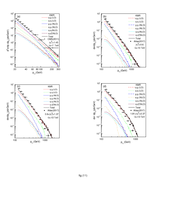
There exist some articles in which the single-photon productions were investigated with the $k_{t}$-factorization formalism KMR1 ; kimber2 ; lips ; lips0 ; lips1 ; lips5 ; lips7 ; lips8 ; lip2007 ; PRD75 , where some conflicts acquire in their calculations. We present some details about these open problems in the section III. It is also noted in the reference PRD75 that the UPDF generated in some of the above references lips ; lips0 ; lips1 ; lips5 ; lips7 ; lips8 ; lip2007 , are not the original version introduced by Kimber et al. KMR nor the one suggested by Martin et al MRW . So these discrepancies should be investigated in details, as it is pointed out in the references PRD75 ; amin . Also, a detailed study of the impact of the NLO sub-processes i.e. the gluon-gluon, quark-gluon and quark-(anti)quark (see the figure 10) are performed and the results are presented for comparison in the section III. It should be noted that this prompt is calculated directly from the NLO perturbation of these processes. However, there are other methods that can indirectly calculate the share of these sub-processes. In these methods, the effects of higher-order perturbation are considered as an effective correction in the LO order tagh1 .

Similar to the discussion made in our photon pair report amin : (1) The off-shell matrix elements that are needed for differential cross-sections calculations are gauge invariance, especially since we are working in the small $x$ region (see, e.g., the references amin ; lips0 for details). (2) There is not any double-counting between the $2\rightarrow 2$ and $2\rightarrow 3$ sub-processes W/Z-LHCb . Because one should consider the KMR or MRW parton densities in the $k_{t}$-factorization formalism correspond to the probability functions similar to the PDF in the collinear case, since all the splittings and the real emissions of the partons, including the last emission, are factorized in the UPDF KIMBER (note that the DGLAP evolution equation derived by integrating over the transverse momentum of partons by ignoring the $k_{t}$ dependent of the PDF). On the other hand, any changes into the UPDF certainly influence the normalization relation between the UPDF and the original PDF (see the equation (24)). However, similar to the reference amin , both points (1) and (2) will be discussed through this paper.

In the following, first, the theoretical framework of prompt single-photon production events (II.1), a brief introduction to the KMR and LO and NLO MRW prescriptions (II.2) and, the experimental conditions (II.3) are presented in the section II. The section III is devoted to our numerical results (III.1) and discussions (III.2). Finally, a brief conclusion is presented in the section IV.

II The Theoretical framework of differential cross-sections prompt single-photon production

II.1 The cross-section

The prompt single-photon production events are an important and useful process to study the PDF. Therefore, it would be interesting to investigate the partonic structure of the proton at each energy while applying the necessary constraints on the experiments. According to the reference D02005 the photons generated in the hard interaction between two partons mainly come from the quark-gluon Compton scattering or the quark-anti-quark annihilation in the hadron collisions. Generally, the photons are so-called prompt, if they are coupled to the interacting quarks 8 ; a2 ; a3 ; a4 . On the other hand, these photons do not produce from the meson decays. Such events are mostly happened in the collinear factorization directly through the $q(\bar{q})+g\longrightarrow\gamma+q(\bar{q})$ and $q+\bar{q}\longrightarrow\gamma+g$ processes D02013 . Usually, in the experimental measurements and theoretical calculations, it is focused on those processes which provide a direct probe of the hard sub-process dynamics, since the produced photons are mostly insensitive to the final-state hadronization D02000 ; 26 ; 27 ; 28 ; 29 ; D02005 ; 31 ; 32 ; 33 ; 33p . At the LO collinear factorization and in the prompt single-photon production where the photon transverse momentum is rather large, the quark-gluon Compton scattering has a larger contribution with respect to the quark-antiquark annihilation process. However, this calculation was done up to the NLO collinear factorization nlosp1 ; jetphox ; nlosp3 ; nlosp4 and the results are in agreement to the data, but some open questions are remaining lip2008 ; re1 ; re2 .

In general, the prompt single-photon production in the hadron-hadron colliders can be described as follows:
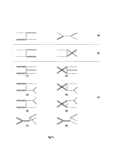
$$A+B\to a+b\to\gamma+X,$$

where $a$ and $b$ are the incoming partons which are emitted by the parent hadrons (A and B). In this work, the sets of LO $2\to 2$ and NLO $2\to 3$ (see the figures 1, 9 and 10 for the LO and NLO level sub-processes and the related discussion about the very small contributions of NLO level processes given in the equation (2) to cross-section in the last part of section (III.2)). The Feynman diagrams are used to demonstrate the partonic sector of the above processes. These are represented as the following two LO partonic and one NLO sub-processes, respectively:

$\displaystyle q(\bar{q})+g$ $\displaystyle\to$ $\displaystyle\gamma+q(\bar{q}),$
$\displaystyle q+\bar{q}$ $\displaystyle\to$ $\displaystyle\gamma+g,$ (1)
$\displaystyle g+g$ $\displaystyle\to$ $\displaystyle\gamma+q+\bar{q},$

namely ”qg” (LO level), ”qq” (LO level) and ”gg” (NLO Level) sub-processes. Also, the share of the other three NLO level sub-paratonic contributions such as, quark-gluon and quark-(anti)quark sub-processes:

$\displaystyle q(\bar{q})+g$ $\displaystyle\to$ $\displaystyle\gamma+q(\bar{q})+g,$
$\displaystyle q(\bar{q})+q(\bar{q})$ $\displaystyle\to$ $\displaystyle\gamma+q(\bar{q})+q(\bar{q}),$
$\displaystyle q+\bar{q}$ $\displaystyle\to$ $\displaystyle\gamma+g+g,$ (2)

are calculated separately (see figure 9, 10 and 11). It should be noted that in the present work, we did not intend to calculate the prompt single-photon production cross-section at the NLO level. Only to show that there is not any double-counting between the $2\to 2$ and $2\to 3$ sub-processes, the $gg$ sub-process which is very small compared to $qg$ and $qq$ sub-processes in the LO level, is added to the all of prompt single-photon production cross-section calculations. However, as we stated above the rest of NLO level sub-processes are discussed in the section (III.2) and the figure 11, which have much smaller effects to the differential cross sections. It is also worth mentioning that for extracting the set of $2\to 3$ NLO Feynman diagrams according to the reference olang ; 113 ; 113-50 ; 113-51 ; 113-52 ; 113-53 , one can use the set of $2\to 2$ LO Feynman diagrams by adding an additional parton emitted from the initial or final partons (collinear factorization approach).

In the case of NLO contributions, the real and virtual corrections should be considered to reach to the finite results and avoid the possible UV-divergence. One can follow this issue for example in the recent review by Konig Konig as well as Passarino-Veltman reduction Veltman ; Boehm (also see, QCDLoop QCD or LoopTools Loop numerical libraries). Some divergences also appear because of the small $k_{t}$ ($<<\mu$) of the outgoing parton Boehm . But since this parton is in the direction of outgoing photons, it is eliminated by excluding the above mentioned regions in our calculation and also implementing isolated and separated cones in this computation. In this work, we applied the same method as the reference jetphox ; amin for the phase space cut.

To carry out the necessary calculations, one should fix the kinematics of these processes. Therefore, the 4-momentum vectors of the colliding protons are written as:

$$P_{1}={\sqrt{s}\over 2}(1,0,0,1),\;\;\;P_{2}={\sqrt{s}\over 2}(1,0,0,-1),$$

where $s$ is the center-of-mass energy.

Using the modified Sudakov decomposition in the high energy light-cone ; Sudakov ,

$$\textbf{k}_{i}=x_{i}\textbf{P}_{i}+\textbf{k}_{i,t},\;\;\;$$ (3)

then, the 4-momenta of the $i^{th}$ parton can be written as a function of the transverse momenta, $k_{i,t}$, and the longitudinal fraction of the momentum, $x_{i}$. These are assumed as inherited parameters for a given parton. Considering the sub-processes in the equations (II.1) and (2) and the conservation law of energy-momentum, the relation between the Bjorken variable ($x$), the transfer momentum ($k_{t}^{i}$), and the rapidity ($y^{i}$) is obtained for the $2\to 2$ sub-processes as:

$$x_{1}={1\over\sqrt{s}}(k_{t}^{\gamma}e^{y_{\gamma}}+m_{t,1}e^{y_{1}}),$$ (4)
$$x_{2}={1\over\sqrt{s}}(k_{t}^{\gamma}e^{-y_{\gamma}}+m_{t,1}e^{-y_{1}})$$ (5)

and for the $2\to 3$ sub-processes as:

$$x_{1}={1\over\sqrt{s}}(k_{t}^{\gamma}e^{y_{\gamma}}+m_{t,1}e^{y_{1}}+m_{t,2}e^{y_{2}}),$$ (6)
$$x_{2}={1\over\sqrt{s}}(k_{t}^{\gamma}e^{-y_{\gamma}}+m_{t,1}e^{-y_{1}}+m_{t,2}e^{-y_{2}}),$$ (7)

where ${y_{\gamma}}$ and ${y_{1}}$ and ${y_{2}}$ are the photon and the outgoing partons rapidities, respectively. Also, $m_{t,1}$ and $m_{t,2}$ are the transverse masses of outgoing partons:

$$m^{2}_{t,i}=m^{2}_{i}+k^{2}_{t,i}.$$ (8)

Note that $m_{t,1}$ becomes $k_{t,1}$ for the gluons light-cone ; Sudakov .

So the incoming partons are off-shell, i.e., they carry transverse momentum and should be described by the corresponding UPDF of the $k_{t}$-factorization. As a result, the prompt single-photon production differential cross-sections in the $k_{t}$-factorization frameworks for the $2\longrightarrow 2$ sub-processes are amin ; lip2007 ; lips0 :

$$\sigma_{qg}(P_{1}+P_{2}\to q(\bar{q})+g\to\gamma+q(\bar{q}))=\int{dk_{1,t}^{2}\over k_{1,t}^{2}}\;{dk_{2,t}^{2}\over k_{2,t}^{2}}dp_{\gamma,t}^{2}\;dy_{\gamma}\;dy_{1}\;{d\varphi_{1}\over 2\pi}\;{d\varphi_{2}\over 2\pi}\;{d\varphi_{\gamma}\over 2\pi}\;\;\times$$
$${|\mathcal{M}(q^{*}(\bar{q}^{*})+g^{*}\rightarrow\gamma+q(\bar{q}))|^{2}\over 16\pi(x_{1}x_{2}s)^{2}}\;f_{q(\bar{q})}(x_{1},k_{1,t}^{2},\mu^{2})\;f_{g}(x_{2},k_{2,t}^{2},\mu^{2}),$$ (9)
$$\sigma_{q\bar{q}}(P_{1}+P_{2}\to q+\bar{q}\to\gamma+g)=\int{dk_{1,t}^{2}\over k_{1,t}^{2}}\;{dk_{2,t}^{2}\over k_{2,t}^{2}}dp_{\gamma,t}^{2}\;dy_{\gamma}\;dy_{1}\;{d\varphi_{1}\over 2\pi}\;{d\varphi_{2}\over 2\pi}\;{d\varphi_{\gamma}\over 2\pi}\;\;\times$$
$${|\mathcal{M}(q^{*}+\bar{q}^{*}\rightarrow\gamma+g)|^{2}\over 16\pi(x_{1}x_{2}s)^{2}}\;f_{q}(x_{1},k_{1,t}^{2},\mu^{2})\;f_{\bar{q}}(x_{2},k_{2,t}^{2},\mu^{2}),$$ (10)

and for the $2\longrightarrow 3$ sub-process is,

$$\sigma_{gg}(P_{1}+P_{2}\to g+g\to\gamma+q+\bar{q})=\int{dk_{1,t}^{2}\over k_{1,t}^{2}}\;{dk_{2,t}^{2}\over k_{2,t}^{2}}\;dp_{\gamma,t}^{2}\;dp_{1,t}^{2}\;dy_{\gamma}\;dy_{1}\;dy_{2}\;\times$$
$${d\varphi_{1}\over 2\pi}\;{d\varphi_{2}\over 2\pi}\;{d\varphi_{\gamma}\over 2\pi}\;{d\psi_{1}\over 2\pi}\times$$
$${|\mathcal{M}(g^{*}+g^{*}\to\gamma+q+\bar{q})|^{2}\over 256\pi^{3}(x_{1}x_{2}s)^{2}}\;f_{g}(x_{1},k_{1,t}^{2},\mu^{2})\;f_{g}(x_{2},k_{2,t}^{2},\mu^{2}),$$ (11)

where the total differential cross-sections can be written as:

$$\sigma_{T}=\sigma_{qg}+\sigma_{q\bar{q}}+\sigma_{gg}$$

The various dispute about the consideration of above $2\longrightarrow 2$ and $2\longrightarrow 3$ sub-processes, as it was mentioned in the introduction will be discussed in the section III amin ; KIMBER ; lips0 ; lip2007 ; W/Z-LHCb ; lips5 .

For calculating the single and double-differential cross-section of prompt single-photon production in the equations (9), (10) and (11), the matrix element squared, $|\mathcal{M}|^{2}$, of the sub-processes of the equation (1) must be calculated. By considering that the incoming partons must be off-shell, the matrix element, $\mathcal{M}$, for the sub processes, which introduced in these equations are defined in the Appendix A and, their Feynman diagrams are displayed in the figure 1. Some of the squared matrix elements are also given in the references lip2007 ; PRD75 ; lips0 . The VEGAS algorithm is considered for performing the multidimensional integration of the total differential cross-section in the equations (9) to (11).

II.2 The choice of UPDF

The UPDF can be directly generated from the PDF, by using different prescriptions. In this work, we use three approaches, the so called KMR KMR , LO and NLO MRW MRW , to obtain the UPDF from the corresponding PDF and substitute them in the equations (9), (10) and (11).

The KMR UPDF are generated such that the partons evolve from the starting PDF parametrization up to the scale $k_{t}$ according to the DGLAP evolution equations KMR . In the KMR method, the partons emit in the single evolution ladder (carrying only the $k_{t}^{2}$ dependency) and get convoluted with the second scale, $\mu^{2}$, at the hard process. The $k_{t}$ is assumed to be depend on the scale $\mu^{2}$, without any real emission, and by summing over the virtual contributions via the Sudakov form factor, $T_{a}(k_{t}^{2},\mu^{2})$. So, the general form of the KMR UPDF are:

$$f_{a}(x,k_{t}^{2},\mu^{2})=T_{a}(k_{t}^{2},\mu^{2})\sum_{b=q,g}\left[{\alpha_{S}(k_{t}^{2})\over 2\pi}\int^{1-\Delta}_{x}dzP_{ab}^{(LO)}(z)b\left({x\over z},k_{t}^{2}\right)\right],$$ (12)

where $T_{a}(k_{t}^{2},\mu^{2})$ are :

$$T_{a}(k_{t}^{2},\mu^{2})=exp\left(-\int_{k_{t}^{2}}^{\mu^{2}}{\alpha_{S}(k^{2})\over 2\pi}{dk^{2}\over k^{2}}\sum_{b=q,g}\int^{1-\Delta}_{0}dz^{\prime}P_{ab}^{(LO)}(z^{\prime})\right).$$ (13)

$T_{a}$ are considered to be unity for $k_{t}>\mu$. $\Delta$ is proposed for the soft gluon and the quark radiations.

To determine $\Delta$, the angular ordering constraint is imposed. The angular ordering originates from the color coherence effects of the gluon radiations KMR . So $\Delta$ is:

$$\Delta={k_{t}\over\mu+k_{t}}.$$

There is also the strong ordering constraint, i.e., $\Delta={k_{t}\over\mu}$ WattWZ ; amin ; O ; kimber2 . $P_{ab}^{(LO)}(z)$ are the LO splitting functions co .

The LO MRW UPDF are similar to the KMR ones, but with the different treatment of the angular ordering constraint. In this approach angular ordering constraint correctly imposed only on the soft gluon radiations, i.e., the diagonal splitting functions $P_{qq}(z)$ and $P_{gg}(z)$ MRW . So, the LO MRW prescription is written as:

$$f_{q}^{LO}(x,k_{t}^{2},\mu^{2})=T_{q}(k_{t}^{2},\mu^{2}){\alpha_{S}(k_{t}^{2})\over 2\pi}\int_{x}^{1}dz\left[P_{qq}^{(LO)}(z){x\over z}q\left({x\over z},k_{t}^{2}\right)\Theta\left({\mu\over\mu+k_{t}}-z\right)\right.$$
$$\left.+P_{qg}^{(LO)}(z){x\over z}g\left({x\over z},k_{t}^{2}\right)\right],$$ (14)

with

$$T_{q}(k_{t}^{2},\mu^{2})=exp\left(-\int_{k_{t}^{2}}^{\mu^{2}}{\alpha_{S}(k^{2})\over 2\pi}{dk^{2}\over k^{2}}\int^{z_{max}}_{0}dz^{\prime}P_{qq}^{(LO)}(z^{\prime})\right),$$ (15)

for the quarks and

$$f_{g}^{LO}(x,k_{t}^{2},\mu^{2})=T_{g}(k_{t}^{2},\mu^{2}){\alpha_{S}(k_{t}^{2})\over 2\pi}\int_{x}^{1}dz\left[P_{gq}^{(LO)}(z)\sum_{q}{x\over z}q\left({x\over z},k_{t}^{2}\right)\right.$$
$$\left.+P_{gg}^{(LO)}(z){x\over z}g\left({x\over z},k_{t}^{2}\right)\Theta\left({\mu\over\mu+k_{t}}-z\right)\right],$$ (16)

with

$$T_{g}(k_{t}^{2},\mu^{2})=exp\left(-\int_{k_{t}^{2}}^{\mu^{2}}{\alpha_{S}(k^{2})\over 2\pi}{dk^{2}\over k^{2}}\left[\int^{z_{max}}_{z_{min}}dz^{\prime}z^{\prime}P_{gg}^{(LO)}(z^{\prime})+n_{f}\int^{1}_{0}dz^{\prime}P_{qg}^{(LO)}(z^{\prime})\right]\right),$$ (17)

for the gluons. In the equations (15) and (17), $z_{max}=1-z_{min}=\mu/(\mu+k_{t})$ WATT .

The Martin et al. MRW also proposed the NLO MRW formalism. This method is based on the DGLAP evolution equation, utilizing the NLO PDF and the corresponding splitting functions MRW . The general form of the NLO MRW UPDF is:

$$f_{a}^{NLO}(x,k_{t}^{2},\mu^{2})=\int_{x}^{1}dzT_{a}\left(k^{2}={k_{t}^{2}\over(1-z)},\mu^{2}\right){\alpha_{S}(k^{2})\over 2\pi}\sum_{b=q,g}\tilde{P}_{ab}^{(LO+NLO)}(z)$$
$$\times b^{NLO}\left({x\over z},k^{2}\right)\Theta\left(1-z-{k_{t}^{2}\over\mu^{2}}\right),$$ (18)

with the ”extended” $NLO$ splitting functions, $\tilde{P}_{ab}^{(i)}(z)$, being defined as:

$$\tilde{P}_{ab}^{(LO+NLO)}(z)=\tilde{P}_{ab}^{(LO)}(z)+{\alpha_{S}\over 2\pi}\tilde{P}_{ab}^{(NLO)}(z),$$ (19)

and

$$\tilde{P}_{ab}^{(i)}(z)=P_{ab}^{i}(z)-\Theta(z-(1-\Delta))\delta_{ab}F^{i}_{ab}P_{ab}(z),$$ (20)

where $i=0$ and $1$ stand for the LO and the NLO, respectively. Also, the angular ordering constraint is defined via the $\Theta(z-(1-\Delta))$ in which $\Delta$ is defined as MRW :

$$\Delta={k\sqrt{1-z}\over k\sqrt{1-z}+\mu}.$$

Finally, the Sudakov form factors in the NLO MRW approach are defined as:

$$T_{q}(k^{2},\mu^{2})=exp\left(-\int_{k^{2}}^{\mu^{2}}{\alpha_{S}(q^{2})\over 2\pi}{dq^{2}\over q^{2}}\int^{1}_{0}dz^{\prime}z^{\prime}\left[\tilde{P}_{qq}^{(0+1)}(z^{\prime})+\tilde{P}_{gq}^{(0+1)}(z^{\prime})\right]\right),$$ (21)
$$T_{g}(k^{2},\mu^{2})=exp\left(-\int_{k^{2}}^{\mu^{2}}{\alpha_{S}(q^{2})\over 2\pi}{dq^{2}\over q^{2}}\int^{1}_{0}dz^{\prime}z^{\prime}\left[\tilde{P}_{gg}^{(0+1)}(z^{\prime})+2n_{f}\tilde{P}_{qg}^{(0+1)}(z^{\prime})\right]\right).$$ (22)

Note that the integral intervals for $dk_{t}$ integration, i.e., the equations (9), (10), are $(0,\infty)$, so one can choose an upper limit for these integrations, say $k_{i,max}$, several times bigger than the hard scale $\mu$. Also, $k_{t,min}=\mu_{0}\sim 1$ $GeV$, is considered as the lower limit that separates the non-perturbative and the perturbative regions, by assuming that,

$${1\over{k_{t}^{2}}}\;f_{a}(x,k_{t}^{2},\mu^{2}){\huge|}_{k_{t}<\mu_{0}}={1\over\mu_{0}^{2}}\;a(x,\mu_{0}^{2})\;T_{a}(\mu_{0}^{2},\mu^{2}).$$ (23)

Eventually, the density of patrons are constant for $k_{t}<\mu_{0}$ at fix $x$ and $\mu$ MRW . For the above calculations, we use the LO-MMHT2014 PDF libraries MMHT for the KMR and the LO MRW UPDF schemes, and the NLO-MMHT2014 PDF libraries MMHT for the NLO MRW formalism. A more complicated extrapolation of the contribution from $k_{t}\leq\mu_{0}$, which ensures the continuity of $f_{a}(x,k_{t}^{2},\mu^{2})\mid_{k_{t}\leq\mu_{0}}$, is given in the references MRW ; WattWZ . This is done by a polynomial expansion of $f_{a}(x,k_{t}^{2},\mu^{2})$ for the requirement of $k_{t}^{2}$ behavior of the UPDF at the small $k_{t}^{2}$.

II.3 The experimental conditions

The fragmentation contributions au are neglected in our calculations, since the isolation cut application D02005 ; CDF2017 reduces these contributions to less than 10 percent of the cross-section. Furthermore, the isolation cuts and additional conditions which preserve our calculations from divergences were specially discussed in the references amin ; lips8 as follows: The isolated-cone is responsible for distinguishing the ”non-prompt decay photons” from the prompt-photons. This constraint requires that the transverse energy $E_{t}^{Hadron}$ (in a cone with the angular radius $R\geq\sqrt{(\eta-\eta^{\gamma})^{2}\;+\;(\phi-\phi_{\gamma})^{2}}$) to be less than a few GeV according to each experiment, where $\eta$ and $\phi$ are the pseudorapidities and the azimuthal angle plane of the hadron and $R\sim 0.4-0.7$, depending on each experimental collaborations. Other constraints, such as the $p_{t}$-threshold of prompt-photons, the pseudo-rapidity regions, etc, are imposed according to the settings of the individual experiments.

III Results and discussions

III.1 The numerical results

We perform a set of numerical calculations for the production of the single-photon at the LHC and TEVATRON colliders, using the equations (9), (10) and (11), within the $k_{t}$-factorization and the different UPDF approaches. The results are separated into the 1.96, 7 and 13 TeV center-of-mass energy ($E_{CM}=\sqrt{s}$), in accordance with the specifications of existing experimental data D02005 ; CDF2017 ; Atlas2017 ; cms . The ratio of our prompt single-photon production differential cross-sections calculation to those of experimental data at each bin ($\cal R$) are separately presented (see the panels (d) of our figures). We also compare our results with those of Monte Carlo simulations which were introduced in the introduction.

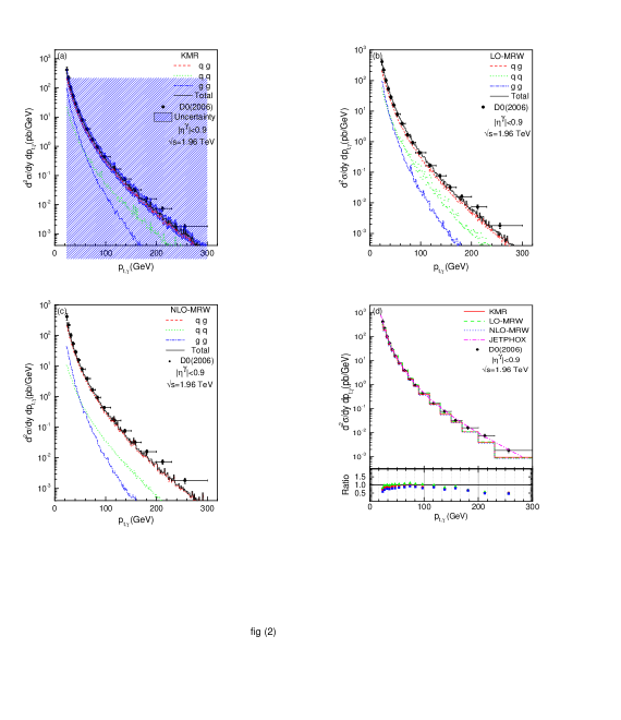
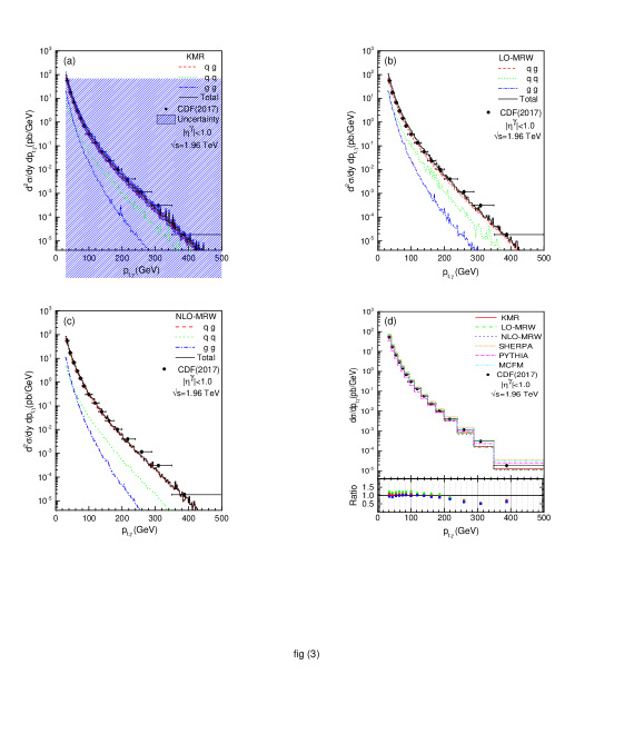
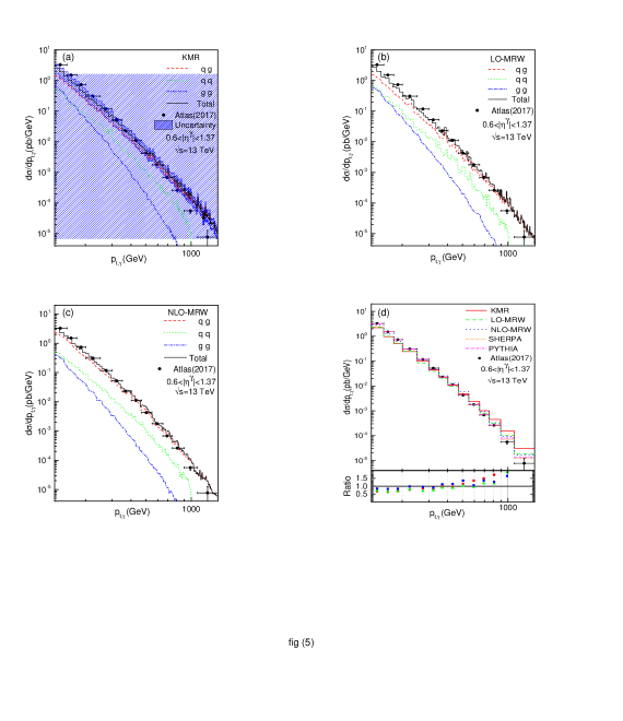
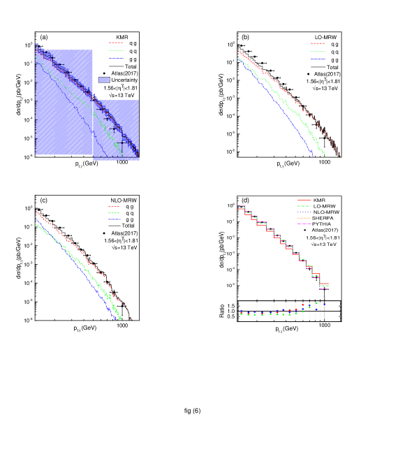
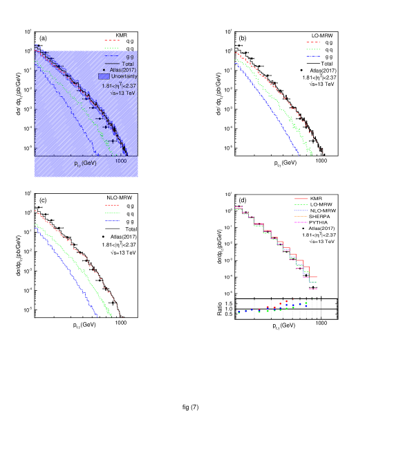
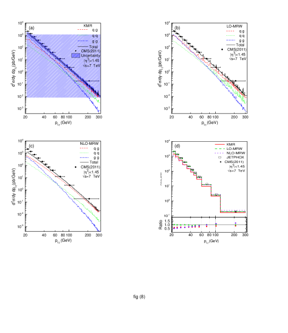
In the figures 2 and 3 the reader is presented with the double differential cross-sections for the production of a single-photon ($d^{2}\sigma/dp_{\gamma,t}dy$) as a function of its transverse momentum ($p_{\gamma,t}$) at $E_{CM}=1.96$ TeV . These results are in accordance with the experimental data of the D0 D02005 and CDF CDF2017 collaborations by applying specific experimental conditions. Similarly, in the figures 4 to 7 and 8, the same results are present for ATLAS measurements Atlas2017 at $E_{CM}=13\;TeV$ and CMS collaboration at $E_{CM}=7$ TeV, respectively.

Within each of these figures, the panel (a) illustrates our results from the utilization of the KMR UPDF, while the panels (b) and (c) exhibit those of the LO and NLO MRW UPDF, respectively. In each of these panels, the contributions from the partonic sub-processes are demonstrated as follows: the red dashed histograms for $q(\bar{q})+g\to\gamma+q(\bar{q})$, the green dotted lines for $q+\bar{q}\to\gamma+g$ and the blue dotted-dash lines for $g+g\to\gamma+q+\bar{q}$. The sum of these contributions for each approaches, i.e., KMR and LO and NLO MRW, are shown with the black solid lines. The corresponding uncertainty regions (see the blue hatched areas in the panel (a)) are calculated, only for the KMR framework, by manipulating the hard-scale $\mu$ by a factor of $2$, i.e., ${1\over 2}\mu$ to $2\mu$. A comparison is also made between all three UPDF approaches and the results of others theoretical calculations, as explained in the corresponding captions of figures (see the panels (d)). Since the experimental results are given at different bins, only in the panels (d) in which the our final differential cross-sections are presented, we average over our results corresponding to each experimental bin.

In the ATLAS collaboration data Atlas2017 , the corresponding measurements were carried out within the following rapidity regions:

  1. 1.

    $|y|<0.6$,

  2. 2.

    $0.6<|y|<1.37$,

  3. 3.

    $1.56<|y|<1.81$,

  4. 4.

    $1.81<|y|<2.37$,

which presented in the figures 4 to 7, respectively.

III.2 Discussions

In the panel (a) of the figures 2 and 3, it is clear that the $qg$ sub-process has large contribution, which confirms the behavior that was reported in the references Atlas2017 ; D02005 . Also, in the small $p_{\gamma,t}$, the contribution of gg sub-processes is larger than those of qq. However, their values become close together around $p_{\gamma,t}=30-50$ GeV, but in the large photon momentum transfer, the portion of qq contribution becomes enhanced with respect to the gg sub-process. The same behavior is observed in the panels (b) and (c), which corresponds to utilizing the LO and NLO MRW $k_{t}$-factorization frameworks. Although, the qg sub-processes still have a dominant contribution, but the crossing interval of gg and qq curves behave differently in each framework. In the panel (d), the final result of three approaches are displayed for the comparison related to the experimental data D02005 . It becomes clear that, there is no significant difference between each $k_{t}$-factorization scheme. Despite differences in the behavior of the partonic sub-processes, these results are relatively similar and in agreement with the experimental findings. However, the small differences which originated from the application of above three schemes, are the effects of different angular ordering constraints. The ratios of our results to those of experimental data are demonstrated at the bottom of these panels ($\cal R$). It is observed that at the small photon transverse momentum regions there are good agreement between the present calculation and the data.
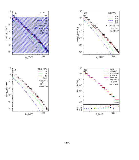
Similar calculations are also made for $E_{CM}=13$ TeV, corresponding to the experimental data of the reference Atlas2017 . The results are presented in the figures 4 to 7. Here, the rapidity region is separated into 4 sectors. The general behaviors of the contributing sub-processes are similar to the $1.96$ TeV case. With increasing the center-of-mass energy of the hadronic collision, the results coming from the NLO MRW framework maintain their relative success in predicting of the experimental data. On the other hand, a tangible difference in the precision of the LO MRW and KMR predictions can be observed.

By moving up between the rapidity regions, it is evident that by increasing the rapidity, the crossing intervals between the qq and gg sub-processes are moved to the small transverse momentum regions. However, they completely disappear in the $1.81<|y|<2.37$ rapidity interval. Actually, the portion of qq contribution is enhanced with respect to the gg sub-processes, while the qg contribution is strongly dominated.

Similar conclusion as above can be made about $\cal R$ in the panels (d) of these figures with this difference that the NLO MRW differential cross-sections are closer to the data.

The same discussion, as the one given above, can be made about the figure 8, but with this difference that the contribution of gg becomes larger in the small photon transverse momentum. This is expected since the center of mass energy is much high with respect to the figures 2 and 3. Note that in the figure 4 to 7, the ATLAS data probing the photon transverse momentum form much lager values, i.e., $125$ GeV. On the other hand, as it was pointed out in the reference amin , in the fragmentation region ($p_{\gamma,t}\leq 30$ GeV ) the LO MRW can support the data much better.

In all of our figures, we also present the results of theoretical prompt single-photon production differential cross-section calculations of different theoretical groups mentioned in the introduction, such as, JETPHOX, SHERPA, PYTHIA and MCFM. A good agreement can be seen between our different $k_{t}$-factorizations calculations and these collinear factorization simulation methods. Similar to our photon pair report they are in the $k_{t}$-angular ordering constraint bound amin

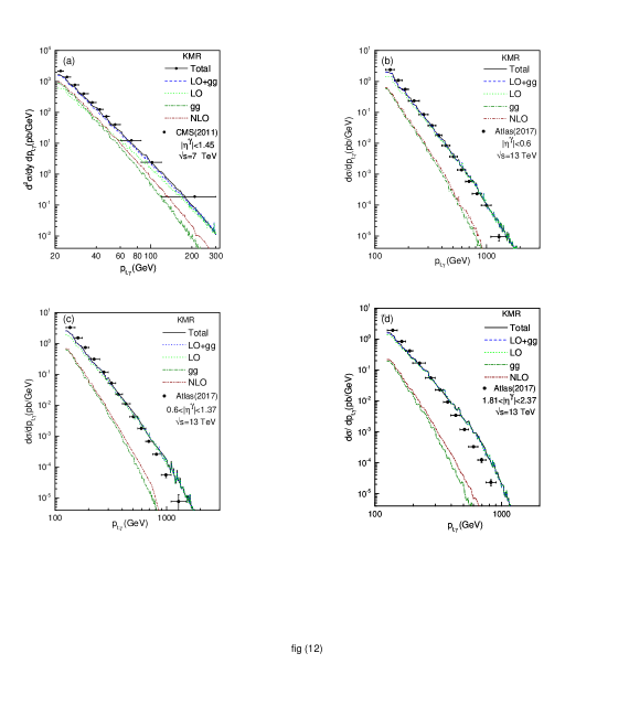
It should be pointed out that beside the NLO gg-fusion process (see the equation (II.1)), the channels $q+g\to q+g+\gamma$ (similar to its Compton LO counterpart), $q^{*}+\bar{q}^{*}\to\gamma+q+\bar{q}$ and $q^{*}+\bar{q}^{*}\to\gamma+g+g$ also appears at the NLO level. On the other hand, when considering the inclusive photon production, the NLO diagrams can contain collinearly enhanced productions that should be factorized properly olang ; 113 ; 113-50 ; 113-51 ; 113-52 ; 113-53 ; light-cone . Therefore, to increase the accuracy of the cross-section calculations, the above sub-processes are also computed at NLO level separately and their diagrams are shown in the figures 9 and 10 (the mathematical formula of the cross-sections for these processes are very similar to that of equation (11)). The result of this calculation is presented in the figure 11 which is based on the specific condition that depicted at each panel. However, the shares of these NLO sub-processes are clearly much less than LO level and gluons-fusion NLO sub-processes, but in over all these portions make the results better in the small photon transverse momentum. In the figure 12, the different contributions of the LO and NLO levels to the differential cross-sections as in the figure 11 are shown separately. It is observed that the NLO sub-processes have very small contributions and the LO level mainly contribute to the cross-sections. However for very small photon transverse momentum the gluons-fusion has sizeable contribution to the cross-sections, as it is pointed out by the CMS collaboration cms . We did not calculate the NLO virtual corrections to the LO quark-gluon process. But they could be the same order as the quark-gluon NLO process, which we have already calculated. On the other hand, one should note that we are not working in the collinear factorization frame work, but the $k_{t}$-factorization. There are quark, antiquark, and gluon degrees of freedom inside of the UPDF such that at LO level one can argue that, e.g. the KMR is a semi-NLO approach.

As it was pointed out in the introduction, we should also discuss about the possible double-counting between our $2\to 2$ and $2\to 3$ sub-processes, which were presented in our results. In some of the references lips ; lips0 ; lips1 ; lips5 ; lips7 ; lips8 ; lip2007 , the $2\to 3$ sub-process is neglected, or if it is considered, only the sea-quarks contributions in the UPDF are omitted on the basis of double-counting, e.g., in the region where the transverse momentum of one of the parton is as large as the hard scale and the additional parton is highly separated in the rapidity, from the hard process (multi-Regge region), while the additional emission in the $2\to 3$ sub-process was subtracted. But, in general, one should consider the KMR or MRW UPDF in the $k_{t}$-factorization calculations corresponds to the non-normalized probability functions. They are used as the weight of the given transition amplitudes (the matrix elements in these cases). The transverse momentum dependence of the UPDF come from considering all possible splittings up to and including the last splitting, see the references KMR ; WattWZ ; WATT ; KMR1 , while the evolution up to the hard scale without a change in the $k_{t}$, due to virtual contributions, is encapsulated in the Sudakov-like survival form factor. Therefore, all splittings and real emissions of the partons, including the last emission, are factorized in the function $f_{g}(x,k_{t}^{2},\mu^{2})$, as its definition. The last emission from the generated UPDF, can not be disassociated and to be count as the part of the $2\to 3$ diagrams W/Z-LHCb ; KIMBER . Recently, a detailed investigation of the above possible double counting is also reported in the reference Guiot , which confirms our conclusions. One should also note that the UPDF have to satisfy the condition given in the identity equation:

$${xa(x,Q^{2})\simeq\int^{Q^{2}}{{dk_{t}^{2}}{k_{t}^{-2}}}}f(x,k^{2}_{t},Q^{2}).$$ (24)

So any changes in the UPDF certainly affect the original PDF definitions and it alters the whole formalism.

However, as it was discussed in the argument in connection to our results, depending on the value of the photon transverse momentum the $2\to 2$ (large $p_{\gamma,t}$) or $2\to 3$ process, i.e., only gluons-fusion (small $p_{\gamma,t}$) make the main contributions to the prompt single-photon production differential cross-sections. To check our results, we also made an approximation and modified our UPDF according to the reference lips5 and found that the results are still in the uncertainty bound region.

In the small x limit, see the reference amin and the reference therein, the off-shell matrix element satisfies the gauge invariance. However, there are reggeization methods to evaluate the off-shell quark density matrix elements which inherently satisfy the gauge invariance in all regions lips1 or the vertex modification KUTAK1 , using the auxiliary photons and quarks. To be sure about the above problem, we checked our result numerically similar to reference lips0 as well as imposing the on-shell matrix elements but with the $k_{t}$-factorization dynamics KMR1 ; kimber2 . We did not find much difference between the off-shell and on-shell matrix elements calculations of differential cross-sections, especially in the large photon momentum transverse, i.e., $\geq 30$ GeV.

IV Conclusion

Throughout this work, using the UPDF of $k_{t}$-factorization, i.e., the KMR and the LO and NLO MRW frameworks, we calculated the rate of prompt single-photon production at the LHC and TEVATRON colliders for the center-of-mass energies of 7 and 13 and 1.96 TeV, respectively. We compared our numerical results against each other and those of the experimental data from the D0, CDF, CMS and ATLAS collaborations. Our aim was generally to illustrate capability of the above UPDF to describe the experimental measurements but do not to increase the precision of such predictions, especially compared to well developed collinear frameworks that are currently used by different collaborations. It was demonstrated that the despite of the simplicity of our model, (on the numerical sense), the UPDF of $k_{t}$-factorization are able to successfully describe the experimental measurements. The further increase in the precision of our calculations is achievable by adding the higher-order and radiation corrections into the matrix elements as well as providing more accurate UPDF via undergoing a complete phenomenological global fit to the existing deep inelastic data WattWZ ; O . Also, for increasing the accuracy, we added the other NLO level sub-processes contributions to the differential cross-sections by using the Feynman rules. These process increased the precision of result only in the small $p_{t,\gamma}$.

As it was mentioned in the sections I and II, the difference in calculating the differential cross-sections with the on-shell or the off-shell matrix element, can affect the results at the small photon momentum transverse regions ($\leq 30$ GeV) and one can conclude that in this region the gauge invariance of the off-shell matrix elements become important. So, on this basis, we are interested to repeat present calculations, using the method introduced in the reference KUTAK1 , concerning the gauge invariance of the off shell matrix element in whole x region. It would be also interesting to investigate the influence of different modifications of UPDF and to use the various angular ordering constraints to examine their behavior in order to check the possible double-counting as well as to consider the differential method to generate the UPDF O ; MRW ; WATT ; WattWZ ; GS . We hope to report these points in our future works.

Acknowledgements.
MM would like to acknowledge the Research Council of University of Tehran for the grants provided for him. RAN sincerely thanks M. Kimber and A. Lipatov for their valuable discussions and comments. We would like to acknowledge the research support of the Iran National Science Foundation (INSF) for their grants.

Appendix A

The various matrix elements of the processes defined in the equations (1) and (2) and the figures 1, 9 and 10, respectively, are given as:
1) $q^{*}(\bar{q}^{*})+g^{*}\to\gamma+q(\bar{q})$ (LO, figure 1):

β„³a=e​g​U¯​(p1)​ta​ϡμ​(k2)​ϡν​(p)​(γμ​kΜΈ1βˆ’pΜΈ+m(k1βˆ’p)2βˆ’m2​γν+γν​kΜΈ1+kΜΈ2+m(k1+k2)2βˆ’m2​γμ)​U​(k1),subscriptβ„³π‘Žπ‘’π‘”Β―π‘ˆsubscript𝑝1superscriptπ‘‘π‘Žsubscriptitalic-Ο΅πœ‡subscriptπ‘˜2subscriptitalic-Ο΅πœˆπ‘superscriptπ›Ύπœ‡subscriptitalic-kΜΈ1italic-pΜΈπ‘šsuperscriptsubscriptπ‘˜1𝑝2superscriptπ‘š2superscriptπ›Ύπœˆsuperscriptπ›Ύπœˆsubscriptitalic-kΜΈ1subscriptitalic-kΜΈ2π‘šsuperscriptsubscriptπ‘˜1subscriptπ‘˜22superscriptπ‘š2superscriptπ›Ύπœ‡π‘ˆsubscriptπ‘˜1\mathcal{M}_{a}=eg\bar{U}(p_{1})t^{a}\epsilon_{\mu}(k_{2})\epsilon_{\nu}(p)(\gamma^{\mu}{\not{k_{1}}-\not{p}+m\over(k_{1}-p)^{2}-m^{2}}\gamma^{\nu}+\gamma^{\nu}{\not{k_{1}}+\not{k_{2}}+m\over(k_{1}+k_{2})^{2}-m^{2}}\gamma^{\mu})U(k_{1}),

2)  $q^{*}+\bar{q}^{*}\to\gamma+g$ (LO, figure 1):

β„³b=e​g​U¯​(k2)​ta​ϡμ​(p1)​ϡν​(p)​(γμ​kΜΈ1βˆ’pΜΈ+m(k1βˆ’p)2βˆ’m2​γν+γν​kΜΈ1βˆ’pΜΈ1+m(k1βˆ’p1)2βˆ’m2​γμ)​U​(k1)subscriptβ„³π‘π‘’π‘”Β―π‘ˆsubscriptπ‘˜2superscriptπ‘‘π‘Žsubscriptitalic-Ο΅πœ‡subscript𝑝1subscriptitalic-Ο΅πœˆπ‘superscriptπ›Ύπœ‡subscriptitalic-kΜΈ1italic-pΜΈπ‘šsuperscriptsubscriptπ‘˜1𝑝2superscriptπ‘š2superscriptπ›Ύπœˆsuperscriptπ›Ύπœˆsubscriptitalic-kΜΈ1subscriptitalic-pΜΈ1π‘šsuperscriptsubscriptπ‘˜1subscript𝑝12superscriptπ‘š2superscriptπ›Ύπœ‡π‘ˆsubscriptπ‘˜1\mathcal{M}_{b}=eg\bar{U}(k_{2})t^{a}\epsilon_{\mu}(p_{1})\epsilon_{\nu}(p)(\gamma^{\mu}{\not{k_{1}}-\not{p}+m\over(k_{1}-p)^{2}-m^{2}}\gamma^{\nu}+\gamma^{\nu}{\not{k_{1}}-\not{p_{1}}+m\over(k_{1}-p_{1})^{2}-m^{2}}\gamma^{\mu})U(k_{1})

3)  $g^{*}+g^{*}\to\gamma+q+\bar{q}$ lips0 (NLO, figure 1):

β„³1=e​g2​U¯​(p1)​tα​γμ​ϡμ​(k1)​pΜΈ1βˆ’kΜΈ1+m(p1βˆ’k1)2βˆ’m2​γξ​ϡξ​(p)​kΜΈ2βˆ’pΜΈ2+m(k2βˆ’p2)2βˆ’m2​tβ​γν​ϡν​(k2)​U​(p2),subscriptβ„³1𝑒superscript𝑔2Β―π‘ˆsubscript𝑝1superscript𝑑𝛼superscriptπ›Ύπœ‡subscriptitalic-Ο΅πœ‡subscriptπ‘˜1subscriptitalic-pΜΈ1subscriptitalic-kΜΈ1π‘šsuperscriptsubscript𝑝1subscriptπ‘˜12superscriptπ‘š2superscriptπ›Ύπœ‰subscriptitalic-Ο΅πœ‰π‘subscriptitalic-kΜΈ2subscriptitalic-pΜΈ2π‘šsuperscriptsubscriptπ‘˜2subscript𝑝22superscriptπ‘š2superscript𝑑𝛽superscriptπ›Ύπœˆsubscriptitalic-ϡ𝜈subscriptπ‘˜2π‘ˆsubscript𝑝2\mathcal{M}_{1}=eg^{2}\bar{U}(p_{1})t^{\alpha}\gamma^{\mu}\epsilon_{\mu}(k_{1}){\not{p_{1}}-\not{k_{1}}+m\over(p_{1}-k_{1})^{2}-m^{2}}\gamma^{\xi}\epsilon_{\xi}(p){\not{k_{2}}-\not{p_{2}}+m\over(k_{2}-p_{2})^{2}-m^{2}}t^{\beta}\gamma^{\nu}\epsilon_{\nu}(k_{2})U(p_{2}),
β„³2=e​g2​U¯​(p1)​tβ​γν​ϡν​(k2)​pΜΈ1βˆ’kΜΈ2+m(p1βˆ’k2)2βˆ’m2​γξ​ϡξ​(p)​kΜΈ1βˆ’pΜΈ2+m(k1βˆ’p2)2βˆ’m2​tα​γμ​ϡμ​(k1)​U​(p2),subscriptβ„³2𝑒superscript𝑔2Β―π‘ˆsubscript𝑝1superscript𝑑𝛽superscriptπ›Ύπœˆsubscriptitalic-ϡ𝜈subscriptπ‘˜2subscriptitalic-pΜΈ1subscriptitalic-kΜΈ2π‘šsuperscriptsubscript𝑝1subscriptπ‘˜22superscriptπ‘š2superscriptπ›Ύπœ‰subscriptitalic-Ο΅πœ‰π‘subscriptitalic-kΜΈ1subscriptitalic-pΜΈ2π‘šsuperscriptsubscriptπ‘˜1subscript𝑝22superscriptπ‘š2superscript𝑑𝛼superscriptπ›Ύπœ‡subscriptitalic-Ο΅πœ‡subscriptπ‘˜1π‘ˆsubscript𝑝2\mathcal{M}_{2}=eg^{2}\bar{U}(p_{1})t^{\beta}\gamma^{\nu}\epsilon_{\nu}(k_{2}){\not{p_{1}}-\not{k_{2}}+m\over(p_{1}-k_{2})^{2}-m^{2}}\gamma^{\xi}\epsilon_{\xi}(p){\not{k_{1}}-\not{p_{2}}+m\over(k_{1}-p_{2})^{2}-m^{2}}t^{\alpha}\gamma^{\mu}\epsilon_{\mu}(k_{1})U(p_{2}),
β„³3=e​g2​U¯​(p1)​tα​γμ​ϡμ​(k1)​pΜΈ1βˆ’kΜΈ1+m(p1βˆ’k1)2βˆ’m2​tβ​γν​ϡν​(k2)β€‹βˆ’pΜΈ2βˆ’pΜΈ+m(βˆ’pβˆ’p2)2βˆ’m2​γξ​ϡξ​(p)​U​(p2),subscriptβ„³3𝑒superscript𝑔2Β―π‘ˆsubscript𝑝1superscript𝑑𝛼superscriptπ›Ύπœ‡subscriptitalic-Ο΅πœ‡subscriptπ‘˜1subscriptitalic-pΜΈ1subscriptitalic-kΜΈ1π‘šsuperscriptsubscript𝑝1subscriptπ‘˜12superscriptπ‘š2superscript𝑑𝛽superscriptπ›Ύπœˆsubscriptitalic-ϡ𝜈subscriptπ‘˜2subscriptitalic-pΜΈ2italic-pΜΈπ‘šsuperscript𝑝subscript𝑝22superscriptπ‘š2superscriptπ›Ύπœ‰subscriptitalic-Ο΅πœ‰π‘π‘ˆsubscript𝑝2\mathcal{M}_{3}=eg^{2}\bar{U}(p_{1})t^{\alpha}\gamma^{\mu}\epsilon_{\mu}(k_{1}){\not{p_{1}}-\not{k_{1}}+m\over(p_{1}-k_{1})^{2}-m^{2}}t^{\beta}\gamma^{\nu}\epsilon_{\nu}(k_{2}){-\not{p_{2}}-\not{p}+m\over(-p-p_{2})^{2}-m^{2}}\gamma^{\xi}\epsilon_{\xi}(p)U(p_{2}),
β„³4=e​g2​U¯​(p1)​tβ​γν​ϡν​(k2)​pΜΈ1βˆ’kΜΈ2+m(p1βˆ’k2)2βˆ’m2​tα​γμ​ϡμ​(k1);βˆ’pΜΈ2βˆ’pΜΈ+m(βˆ’pβˆ’p2)2βˆ’m2​γξ​ϡξ​(p)​U​(p2),subscriptβ„³4𝑒superscript𝑔2Β―π‘ˆsubscript𝑝1superscript𝑑𝛽superscriptπ›Ύπœˆsubscriptitalic-ϡ𝜈subscriptπ‘˜2subscriptitalic-pΜΈ1subscriptitalic-kΜΈ2π‘šsuperscriptsubscript𝑝1subscriptπ‘˜22superscriptπ‘š2superscript𝑑𝛼superscriptπ›Ύπœ‡subscriptitalic-Ο΅πœ‡subscriptπ‘˜1subscriptitalic-pΜΈ2italic-pΜΈπ‘šsuperscript𝑝subscript𝑝22superscriptπ‘š2superscriptπ›Ύπœ‰subscriptitalic-Ο΅πœ‰π‘π‘ˆsubscript𝑝2\mathcal{M}_{4}=eg^{2}\bar{U}(p_{1})t^{\beta}\gamma^{\nu}\epsilon_{\nu}(k_{2}){\not{p_{1}}-\not{k_{2}}+m\over(p_{1}-k_{2})^{2}-m^{2}}t^{\alpha}\gamma^{\mu}\epsilon_{\mu}(k_{1});\ {-\not{p_{2}}-\not{p}+m\over(-p-p_{2})^{2}-m^{2}}\gamma^{\xi}\epsilon_{\xi}(p)U(p_{2}),
β„³5=e​g2​U¯​(p1)​γξ​ϡξ​(p)​pΜΈ1+pΜΈ+m(p1+p)2βˆ’m2​tα​γμ​ϡμ​(k1)​kΜΈ2βˆ’pΜΈ2+m(k2βˆ’p2)2βˆ’m2​tβ​γν​ϡν​(k2)​U​(p2),subscriptβ„³5𝑒superscript𝑔2Β―π‘ˆsubscript𝑝1superscriptπ›Ύπœ‰subscriptitalic-Ο΅πœ‰π‘subscriptitalic-pΜΈ1italic-pΜΈπ‘šsuperscriptsubscript𝑝1𝑝2superscriptπ‘š2superscript𝑑𝛼superscriptπ›Ύπœ‡subscriptitalic-Ο΅πœ‡subscriptπ‘˜1subscriptitalic-kΜΈ2subscriptitalic-pΜΈ2π‘šsuperscriptsubscriptπ‘˜2subscript𝑝22superscriptπ‘š2superscript𝑑𝛽superscriptπ›Ύπœˆsubscriptitalic-ϡ𝜈subscriptπ‘˜2π‘ˆsubscript𝑝2\mathcal{M}_{5}=eg^{2}\bar{U}(p_{1})\gamma^{\xi}\epsilon_{\xi}(p){\not{p_{1}}+\not{p}+m\over(p_{1}+p)^{2}-m^{2}}t^{\alpha}\gamma^{\mu}\epsilon_{\mu}(k_{1}){\not{k_{2}}-\not{p_{2}}+m\over(k_{2}-p_{2})^{2}-m^{2}}t^{\beta}\gamma^{\nu}\epsilon_{\nu}(k_{2})U(p_{2}),
β„³6=e​g2​U¯​(p1)​γξ​ϡξ​(p)​pΜΈ1+pΜΈ+m(p1+p)2βˆ’m2​tβ​γν​ϡν​(k2)​kΜΈ1βˆ’pΜΈ2+m(k1βˆ’p2)2βˆ’m2​tα​γμ​ϡμ​(k1)​U​(p2),subscriptβ„³6𝑒superscript𝑔2Β―π‘ˆsubscript𝑝1superscriptπ›Ύπœ‰subscriptitalic-Ο΅πœ‰π‘subscriptitalic-pΜΈ1italic-pΜΈπ‘šsuperscriptsubscript𝑝1𝑝2superscriptπ‘š2superscript𝑑𝛽superscriptπ›Ύπœˆsubscriptitalic-ϡ𝜈subscriptπ‘˜2subscriptitalic-kΜΈ1subscriptitalic-pΜΈ2π‘šsuperscriptsubscriptπ‘˜1subscript𝑝22superscriptπ‘š2superscript𝑑𝛼superscriptπ›Ύπœ‡subscriptitalic-Ο΅πœ‡subscriptπ‘˜1π‘ˆsubscript𝑝2\mathcal{M}_{6}=eg^{2}\bar{U}(p_{1})\gamma^{\xi}\epsilon_{\xi}(p){\not{p_{1}}+\not{p}+m\over(p_{1}+p)^{2}-m^{2}}t^{\beta}\gamma^{\nu}\epsilon_{\nu}(k_{2}){\not{k_{1}}-\not{p_{2}}+m\over(k_{1}-p_{2})^{2}-m^{2}}t^{\alpha}\gamma^{\mu}\epsilon_{\mu}(k_{1})U(p_{2}),
β„³7=βˆ’e​g2​U¯​(p1)​γρ​Cμ​ν​ρ​(k1,k2,βˆ’k1βˆ’k2)​ϡμ​(k1)​ϡν​(k2)(k1+k2)2​fa​b​c​tcβ€‹βˆ’pΜΈ2βˆ’pΜΈ+m(βˆ’p2βˆ’p)2βˆ’m2​γξ​ϡξ​(p)​U​(p2),subscriptβ„³7𝑒superscript𝑔2Β―π‘ˆsubscript𝑝1superscriptπ›ΎπœŒsuperscriptπΆπœ‡πœˆπœŒsubscriptπ‘˜1subscriptπ‘˜2subscriptπ‘˜1subscriptπ‘˜2subscriptitalic-Ο΅πœ‡subscriptπ‘˜1subscriptitalic-ϡ𝜈subscriptπ‘˜2superscriptsubscriptπ‘˜1subscriptπ‘˜22superscriptπ‘“π‘Žπ‘π‘superscript𝑑𝑐subscriptitalic-pΜΈ2italic-pΜΈπ‘šsuperscriptsubscript𝑝2𝑝2superscriptπ‘š2superscriptπ›Ύπœ‰subscriptitalic-Ο΅πœ‰π‘π‘ˆsubscript𝑝2\mathcal{M}_{7}=-eg^{2}\bar{U}(p_{1})\gamma^{\rho}C^{\mu\nu\rho}(k_{1},k_{2},-k_{1}-k_{2}){\epsilon_{\mu}(k_{1})\epsilon_{\nu}(k_{2})\over(k_{1}+k_{2})^{2}}f^{abc}t^{c}{-\not{p_{2}}-\not{p}+m\over(-p_{2}-p)^{2}-m^{2}}\gamma^{\xi}\epsilon_{\xi}(p)U(p_{2}),
β„³8=βˆ’e​g2​U¯​(p1)​γξ​ϡξ​(p)​pΜΈ1+pΜΈ+m(p1+p)2βˆ’m2​γρ​Cμ​ν​ρ​(k1,k2,βˆ’k1βˆ’k2)​ϡμ​(k1)​ϡν​(k2)(k1+k2)2​fa​b​c​tc​U​(p2).subscriptβ„³8𝑒superscript𝑔2Β―π‘ˆsubscript𝑝1superscriptπ›Ύπœ‰subscriptitalic-Ο΅πœ‰π‘subscriptitalic-pΜΈ1italic-pΜΈπ‘šsuperscriptsubscript𝑝1𝑝2superscriptπ‘š2superscriptπ›ΎπœŒsuperscriptπΆπœ‡πœˆπœŒsubscriptπ‘˜1subscriptπ‘˜2subscriptπ‘˜1subscriptπ‘˜2subscriptitalic-Ο΅πœ‡subscriptπ‘˜1subscriptitalic-ϡ𝜈subscriptπ‘˜2superscriptsubscriptπ‘˜1subscriptπ‘˜22superscriptπ‘“π‘Žπ‘π‘superscriptπ‘‘π‘π‘ˆsubscript𝑝2\mathcal{M}_{8}=-eg^{2}\bar{U}(p_{1})\gamma^{\xi}\epsilon_{\xi}(p){\not{p_{1}}+\not{p}+m\over(p_{1}+p)^{2}-m^{2}}\gamma^{\rho}C^{\mu\nu\rho}(k_{1},k_{2},-k_{1}-k_{2}){\epsilon_{\mu}(k_{1})\epsilon_{\nu}(k_{2})\over(k_{1}+k_{2})^{2}}f^{abc}t^{c}U(p_{2}).

4)  $q^{*}(\bar{q}^{*})+g^{*}\to\gamma+q(\bar{q})+g$, (NLO, figure 9):

β„³1=e​g2​U¯​(p1)​γξ​ϡξ​(p)​pΜΈ1+pΜΈ+m(p1+p)2βˆ’m2​tα​γμ​ϡμ​(p2)​kΜΈ1+kΜΈ2+m(k1+k2)2βˆ’m2​tβ​γν​ϡν​(k2)​U​(k1),subscriptβ„³1𝑒superscript𝑔2Β―π‘ˆsubscript𝑝1superscriptπ›Ύπœ‰subscriptitalic-Ο΅πœ‰π‘subscriptitalic-pΜΈ1italic-pΜΈπ‘šsuperscriptsubscript𝑝1𝑝2superscriptπ‘š2superscript𝑑𝛼superscriptπ›Ύπœ‡subscriptitalic-Ο΅πœ‡subscript𝑝2subscriptitalic-kΜΈ1subscriptitalic-kΜΈ2π‘šsuperscriptsubscriptπ‘˜1subscriptπ‘˜22superscriptπ‘š2superscript𝑑𝛽superscriptπ›Ύπœˆsubscriptitalic-ϡ𝜈subscriptπ‘˜2π‘ˆsubscriptπ‘˜1\mathcal{M}_{1}=eg^{2}\bar{U}(p_{1})\gamma^{\xi}\epsilon_{\xi}(p){\not{p_{1}}+\not{p}+m\over(p_{1}+p)^{2}-m^{2}}t^{\alpha}\gamma^{\mu}\epsilon_{\mu}(p_{2}){\not{k_{1}}+\not{k_{2}}+m\over(k_{1}+k_{2})^{2}-m^{2}}t^{\beta}\gamma^{\nu}\epsilon_{\nu}(k_{2})U(k_{1}),
β„³2=e​g2​U¯​(p1)​tα​γμ​ϡμ​(p2)​pΜΈ1+pΜΈ2+m(p1+p2)2βˆ’m2​γξ​ϡξ​(p)​kΜΈ1+kΜΈ2+m(k1+k2)2βˆ’m2​tβ​γν​ϡν​(k2)​U​(k1),subscriptβ„³2𝑒superscript𝑔2Β―π‘ˆsubscript𝑝1superscript𝑑𝛼superscriptπ›Ύπœ‡subscriptitalic-Ο΅πœ‡subscript𝑝2subscriptitalic-pΜΈ1subscriptitalic-pΜΈ2π‘šsuperscriptsubscript𝑝1subscript𝑝22superscriptπ‘š2superscriptπ›Ύπœ‰subscriptitalic-Ο΅πœ‰π‘subscriptitalic-kΜΈ1subscriptitalic-kΜΈ2π‘šsuperscriptsubscriptπ‘˜1subscriptπ‘˜22superscriptπ‘š2superscript𝑑𝛽superscriptπ›Ύπœˆsubscriptitalic-ϡ𝜈subscriptπ‘˜2π‘ˆsubscriptπ‘˜1\mathcal{M}_{2}=eg^{2}\bar{U}(p_{1})t^{\alpha}\gamma^{\mu}\epsilon_{\mu}(p_{2}){\not{p_{1}}+\not{p_{2}}+m\over(p_{1}+p_{2})^{2}-m^{2}}\gamma^{\xi}\epsilon_{\xi}(p){\not{k_{1}}+\not{k_{2}}+m\over(k_{1}+k_{2})^{2}-m^{2}}t^{\beta}\gamma^{\nu}\epsilon_{\nu}(k_{2})U(k_{1}),
β„³3=e​g2​U¯​(p1)​tα​γμ​ϡμ​(p2)​pΜΈ1+pΜΈ2+m(p1+p2)2βˆ’m2​tβ​γν​ϡν​(k2)​kΜΈ1βˆ’pΜΈ+m(k1βˆ’p)2βˆ’m2​γξ​ϡξ​(p)​U​(k1),subscriptβ„³3𝑒superscript𝑔2Β―π‘ˆsubscript𝑝1superscript𝑑𝛼superscriptπ›Ύπœ‡subscriptitalic-Ο΅πœ‡subscript𝑝2subscriptitalic-pΜΈ1subscriptitalic-pΜΈ2π‘šsuperscriptsubscript𝑝1subscript𝑝22superscriptπ‘š2superscript𝑑𝛽superscriptπ›Ύπœˆsubscriptitalic-ϡ𝜈subscriptπ‘˜2subscriptitalic-kΜΈ1italic-pΜΈπ‘šsuperscriptsubscriptπ‘˜1𝑝2superscriptπ‘š2superscriptπ›Ύπœ‰subscriptitalic-Ο΅πœ‰π‘π‘ˆsubscriptπ‘˜1\mathcal{M}_{3}=eg^{2}\bar{U}(p_{1})t^{\alpha}\gamma^{\mu}\epsilon_{\mu}(p_{2}){\not{p_{1}}+\not{p_{2}}+m\over(p_{1}+p_{2})^{2}-m^{2}}t^{\beta}\gamma^{\nu}\epsilon_{\nu}(k_{2}){\not{k_{1}}-\not{p}+m\over(k_{1}-p)^{2}-m^{2}}\gamma^{\xi}\epsilon_{\xi}(p)U(k_{1}),
β„³4=e​g2​U¯​(p1)​tβ​γν​ϡν​(k2)​kΜΈ2βˆ’pΜΈ1+m(k2βˆ’p1)2βˆ’m2​γξ​ϡξ​(p)​kΜΈ1βˆ’pΜΈ2+m(k1βˆ’p2)2βˆ’m2​tα​γμ​ϡμ​(p2)​U​(k1),subscriptβ„³4𝑒superscript𝑔2Β―π‘ˆsubscript𝑝1superscript𝑑𝛽superscriptπ›Ύπœˆsubscriptitalic-ϡ𝜈subscriptπ‘˜2subscriptitalic-kΜΈ2subscriptitalic-pΜΈ1π‘šsuperscriptsubscriptπ‘˜2subscript𝑝12superscriptπ‘š2superscriptπ›Ύπœ‰subscriptitalic-Ο΅πœ‰π‘subscriptitalic-kΜΈ1subscriptitalic-pΜΈ2π‘šsuperscriptsubscriptπ‘˜1subscript𝑝22superscriptπ‘š2superscript𝑑𝛼superscriptπ›Ύπœ‡subscriptitalic-Ο΅πœ‡subscript𝑝2π‘ˆsubscriptπ‘˜1\mathcal{M}_{4}=eg^{2}\bar{U}(p_{1})t^{\beta}\gamma^{\nu}\epsilon_{\nu}(k_{2}){\not{k_{2}}-\not{p_{1}}+m\over(k_{2}-p_{1})^{2}-m^{2}}\gamma^{\xi}\epsilon_{\xi}(p){\not{k_{1}}-\not{p_{2}}+m\over(k_{1}-p_{2})^{2}-m^{2}}t^{\alpha}\gamma^{\mu}\epsilon_{\mu}(p_{2})U(k_{1}),
β„³5=e​g2​U¯​(p1)​tβ​γν​ϡν​(k2)​kΜΈ2βˆ’pΜΈ2+m(k2βˆ’p2)2βˆ’m2​tα​γμ​ϡμ​(p2)​kΜΈ1βˆ’pΜΈ+m(k1βˆ’p)2βˆ’m2​γξ​ϡξ​(p)​U​(k1),subscriptβ„³5𝑒superscript𝑔2Β―π‘ˆsubscript𝑝1superscript𝑑𝛽superscriptπ›Ύπœˆsubscriptitalic-ϡ𝜈subscriptπ‘˜2subscriptitalic-kΜΈ2subscriptitalic-pΜΈ2π‘šsuperscriptsubscriptπ‘˜2subscript𝑝22superscriptπ‘š2superscript𝑑𝛼superscriptπ›Ύπœ‡subscriptitalic-Ο΅πœ‡subscript𝑝2subscriptitalic-kΜΈ1italic-pΜΈπ‘šsuperscriptsubscriptπ‘˜1𝑝2superscriptπ‘š2superscriptπ›Ύπœ‰subscriptitalic-Ο΅πœ‰π‘π‘ˆsubscriptπ‘˜1\mathcal{M}_{5}=eg^{2}\bar{U}(p_{1})t^{\beta}\gamma^{\nu}\epsilon_{\nu}(k_{2}){\not{k_{2}}-\not{p_{2}}+m\over(k_{2}-p_{2})^{2}-m^{2}}t^{\alpha}\gamma^{\mu}\epsilon_{\mu}(p_{2}){\not{k_{1}}-\not{p}+m\over(k_{1}-p)^{2}-m^{2}}\gamma^{\xi}\epsilon_{\xi}(p)U(k_{1}),
β„³6=βˆ’e​g2​U¯​(p1)​γξ​ϡξ​(p)​pΜΈ1+pΜΈ+m(p1+p)2βˆ’m2​γρ​Cμ​ν​ρ​(k1,k2,p)​ϡμ​(p2)​ϡν​(k2)(k1βˆ’p1)2​fa​b​c​tc​U​(k1),subscriptβ„³6𝑒superscript𝑔2Β―π‘ˆsubscript𝑝1superscriptπ›Ύπœ‰subscriptitalic-Ο΅πœ‰π‘subscriptitalic-pΜΈ1italic-pΜΈπ‘šsuperscriptsubscript𝑝1𝑝2superscriptπ‘š2superscriptπ›ΎπœŒsuperscriptπΆπœ‡πœˆπœŒsubscriptπ‘˜1subscriptπ‘˜2𝑝subscriptitalic-Ο΅πœ‡subscript𝑝2subscriptitalic-ϡ𝜈subscriptπ‘˜2superscriptsubscriptπ‘˜1subscript𝑝12superscriptπ‘“π‘Žπ‘π‘superscriptπ‘‘π‘π‘ˆsubscriptπ‘˜1\mathcal{M}_{6}=-eg^{2}\bar{U}(p_{1})\gamma^{\xi}\epsilon_{\xi}(p){\not{p_{1}}+\not{p}+m\over(p_{1}+p)^{2}-m^{2}}\gamma^{\rho}C^{\mu\nu\rho}(k_{1},k_{2},p){\epsilon_{\mu}(p_{2})\epsilon_{\nu}(k_{2})\over(k_{1}-p_{1})^{2}}f^{abc}t^{c}U(k_{1}),
β„³7=e​g2​U¯​(p1)​γξ​ϡξ​(p)​kΜΈ1+pΜΈ+m(k1+p)2βˆ’m2​tβ​γν​ϡν​(k2)​kΜΈ1βˆ’pΜΈ2+m(k1βˆ’p2)2βˆ’m2​tα​γμ​ϡμ​(p2)​U​(k1),subscriptβ„³7𝑒superscript𝑔2Β―π‘ˆsubscript𝑝1superscriptπ›Ύπœ‰subscriptitalic-Ο΅πœ‰π‘subscriptitalic-kΜΈ1italic-pΜΈπ‘šsuperscriptsubscriptπ‘˜1𝑝2superscriptπ‘š2superscript𝑑𝛽superscriptπ›Ύπœˆsubscriptitalic-ϡ𝜈subscriptπ‘˜2subscriptitalic-kΜΈ1subscriptitalic-pΜΈ2π‘šsuperscriptsubscriptπ‘˜1subscript𝑝22superscriptπ‘š2superscript𝑑𝛼superscriptπ›Ύπœ‡subscriptitalic-Ο΅πœ‡subscript𝑝2π‘ˆsubscriptπ‘˜1\mathcal{M}_{7}=eg^{2}\bar{U}(p_{1})\gamma^{\xi}\epsilon_{\xi}(p){\not{k_{1}}+\not{p}+m\over(k_{1}+p)^{2}-m^{2}}t^{\beta}\gamma^{\nu}\epsilon_{\nu}(k_{2}){\not{k_{1}}-\not{p_{2}}+m\over(k_{1}-p_{2})^{2}-m^{2}}t^{\alpha}\gamma^{\mu}\epsilon_{\mu}(p_{2})U(k_{1}),
β„³8=βˆ’e​g2​U​(k1)​γξ​ϡξ​(p)​kΜΈ1βˆ’pΜΈ+m(k1βˆ’p)2βˆ’m2​γρ​Cμ​ν​ρ​(k1,k2,p)​ϡμ​(p2)​ϡν​(k2)(k1βˆ’p1)2​fa​b​c​tc​U¯​(p1),subscriptβ„³8𝑒superscript𝑔2π‘ˆsubscriptπ‘˜1superscriptπ›Ύπœ‰subscriptitalic-Ο΅πœ‰π‘subscriptitalic-kΜΈ1italic-pΜΈπ‘šsuperscriptsubscriptπ‘˜1𝑝2superscriptπ‘š2superscriptπ›ΎπœŒsuperscriptπΆπœ‡πœˆπœŒsubscriptπ‘˜1subscriptπ‘˜2𝑝subscriptitalic-Ο΅πœ‡subscript𝑝2subscriptitalic-ϡ𝜈subscriptπ‘˜2superscriptsubscriptπ‘˜1subscript𝑝12superscriptπ‘“π‘Žπ‘π‘superscriptπ‘‘π‘Β―π‘ˆsubscript𝑝1\mathcal{M}_{8}=-eg^{2}U(k_{1})\gamma^{\xi}\epsilon_{\xi}(p){\not{k_{1}}-\not{p}+m\over(k_{1}-p)^{2}-m^{2}}\gamma^{\rho}C^{\mu\nu\rho}(k_{1},k_{2},p){\epsilon_{\mu}(p_{2})\epsilon_{\nu}(k_{2})\over(k_{1}-p_{1})^{2}}f^{abc}t^{c}\bar{U}(p_{1}),

5)  $q^{*}+\bar{q}^{*}\to\gamma+q+\bar{q}$ (NLO, figure 10)

β„³a​.1=e​g2​U¯​(p2)​γμ​ϡμ​(p)​pΜΈ2+pΜΈ+m(p2+p)2βˆ’m2​U​(p1)​tα​γξ​gξ​ν​δα​β(k1+k2)2​tβ​U¯​(k2)​γν​U​(k1),subscriptβ„³π‘Ž.1𝑒superscript𝑔2Β―π‘ˆsubscript𝑝2superscriptπ›Ύπœ‡subscriptitalic-Ο΅πœ‡π‘subscriptitalic-pΜΈ2italic-pΜΈπ‘šsuperscriptsubscript𝑝2𝑝2superscriptπ‘š2π‘ˆsubscript𝑝1superscript𝑑𝛼superscriptπ›Ύπœ‰superscriptπ‘”πœ‰πœˆsuperscript𝛿𝛼𝛽superscriptsubscriptπ‘˜1subscriptπ‘˜22superscriptπ‘‘π›½Β―π‘ˆsubscriptπ‘˜2superscriptπ›Ύπœˆπ‘ˆsubscriptπ‘˜1\mathcal{M}_{a.1}=eg^{2}\bar{U}(p_{2})\gamma^{\mu}\epsilon_{\mu}(p){\not{p_{2}}+\not{p}+m\over(p_{2}+p)^{2}-m^{2}}U(p_{1})t^{\alpha}\gamma^{\xi}{g^{\xi\nu}\delta^{\alpha\beta}\over(k_{1}+k_{2})^{2}}t^{\beta}\bar{U}(k_{2})\gamma^{\nu}U(k_{1}),
β„³a​.2=e​g2​U¯​(p2)​γμ​ϡμ​(p)​pΜΈ2+pΜΈ+m(p2+p)2βˆ’m2​U¯​(k2)​tβ​γν​gξ​ν​δα​β(k​1βˆ’p​1)2​U​(p1)​tα​γξ​U​(k1),subscriptβ„³π‘Ž.2𝑒superscript𝑔2Β―π‘ˆsubscript𝑝2superscriptπ›Ύπœ‡subscriptitalic-Ο΅πœ‡π‘subscriptitalic-pΜΈ2italic-pΜΈπ‘šsuperscriptsubscript𝑝2𝑝2superscriptπ‘š2Β―π‘ˆsubscriptπ‘˜2superscript𝑑𝛽superscriptπ›Ύπœˆsuperscriptπ‘”πœ‰πœˆsuperscript𝛿𝛼𝛽superscriptπ‘˜1𝑝12π‘ˆsubscript𝑝1superscript𝑑𝛼superscriptπ›Ύπœ‰π‘ˆsubscriptπ‘˜1\mathcal{M}_{a.2}=eg^{2}\bar{U}(p_{2})\gamma^{\mu}\epsilon_{\mu}(p){\not{p_{2}}+\not{p}+m\over(p_{2}+p)^{2}-m^{2}}\bar{U}(k_{2})t^{\beta}\gamma^{\nu}{g^{\xi\nu}\delta^{\alpha\beta}\over(k1-p1)^{2}}U(p_{1})t^{\alpha}\gamma^{\xi}U(k_{1}),
β„³a​.3=e​g2​U¯​(p2)​tα​γξ​U​(p1)​gξ​ν​δα​β(p2+p1)2​U¯​(k2)​tβ​γν​kΜΈ1βˆ’pΜΈ+m(k1βˆ’p)2βˆ’m2​ϡμ​(p)​γμ​U​(k1),subscriptβ„³π‘Ž.3𝑒superscript𝑔2Β―π‘ˆsubscript𝑝2superscript𝑑𝛼superscriptπ›Ύπœ‰π‘ˆsubscript𝑝1superscriptπ‘”πœ‰πœˆsuperscript𝛿𝛼𝛽superscriptsubscript𝑝2subscript𝑝12Β―π‘ˆsubscriptπ‘˜2superscript𝑑𝛽superscriptπ›Ύπœˆsubscriptitalic-kΜΈ1italic-pΜΈπ‘šsuperscriptsubscriptπ‘˜1𝑝2superscriptπ‘š2subscriptitalic-Ο΅πœ‡π‘superscriptπ›Ύπœ‡π‘ˆsubscriptπ‘˜1\mathcal{M}_{a.3}=eg^{2}\bar{U}(p_{2})t^{\alpha}\gamma^{\xi}U(p_{1}){g^{\xi\nu}\delta^{\alpha\beta}\over(p_{2}+p_{1})^{2}}\bar{U}(k_{2})t^{\beta}\gamma^{\nu}{\not{k_{1}}-\not{p}+m\over(k_{1}-p)^{2}-m^{2}}\epsilon_{\mu}(p)\gamma^{\mu}U(k_{1}),
β„³a​.4=e​g2​U​(p1)​γξ​ϡξ​(p)​pΜΈ1+pΜΈ+m(p1+p)2βˆ’m2​U¯​(p2)​γμ​tα​gμ​ν​δα​β(k2+k1)2​tβ​U¯​(k2)​γξ​U​(k1),subscriptβ„³π‘Ž.4𝑒superscript𝑔2π‘ˆsubscript𝑝1superscriptπ›Ύπœ‰subscriptitalic-Ο΅πœ‰π‘subscriptitalic-pΜΈ1italic-pΜΈπ‘šsuperscriptsubscript𝑝1𝑝2superscriptπ‘š2Β―π‘ˆsubscript𝑝2superscriptπ›Ύπœ‡superscript𝑑𝛼superscriptπ‘”πœ‡πœˆsuperscript𝛿𝛼𝛽superscriptsubscriptπ‘˜2subscriptπ‘˜12superscriptπ‘‘π›½Β―π‘ˆsubscriptπ‘˜2superscriptπ›Ύπœ‰π‘ˆsubscriptπ‘˜1\mathcal{M}_{a.4}=eg^{2}U(p_{1})\gamma^{\xi}\epsilon_{\xi}(p){\not{p_{1}}+\not{p}+m\over(p_{1}+p)^{2}-m^{2}}\bar{U}(p_{2})\gamma^{\mu}t^{\alpha}{g^{\mu\nu}\delta^{\alpha\beta}\over(k_{2}+k_{1})^{2}}t^{\beta}\bar{U}(k_{2})\gamma^{\xi}U(k_{1}),
β„³a​.5=e​g2​U​(p1)​γξ​tα​U​(k1)​gμ​ξ​δα​β(k1βˆ’p1)2​U¯​(p2)​γμ​tβ​kΜΈ2βˆ’pΜΈ+m(k2βˆ’p)2βˆ’m2​ϡν​(p)​γν​U¯​(k2),subscriptβ„³π‘Ž.5𝑒superscript𝑔2π‘ˆsubscript𝑝1superscriptπ›Ύπœ‰superscriptπ‘‘π›Όπ‘ˆsubscriptπ‘˜1superscriptπ‘”πœ‡πœ‰superscript𝛿𝛼𝛽superscriptsubscriptπ‘˜1subscript𝑝12Β―π‘ˆsubscript𝑝2superscriptπ›Ύπœ‡superscript𝑑𝛽subscriptitalic-kΜΈ2italic-pΜΈπ‘šsuperscriptsubscriptπ‘˜2𝑝2superscriptπ‘š2subscriptitalic-Ο΅πœˆπ‘superscriptπ›ΎπœˆΒ―π‘ˆsubscriptπ‘˜2\mathcal{M}_{a.5}=eg^{2}U(p_{1})\gamma^{\xi}t^{\alpha}U(k_{1}){g^{\mu\xi}\delta^{\alpha\beta}\over(k_{1}-p_{1})^{2}}\bar{U}(p_{2})\gamma^{\mu}t^{\beta}{\not{k_{2}}-\not{p}+m\over(k_{2}-p)^{2}-m^{2}}\epsilon_{\nu}(p)\gamma^{\nu}\bar{U}(k_{2}),
β„³a​.6=e​g2​U¯​(p2)​tα​γξ​U​(p1)​gξ​ν​δα​β(p2+p1)2​tβ​U​(k1)​γν​kΜΈ1βˆ’pΜΈ+m(k1βˆ’p)2βˆ’m2​γμ​ϡμ​(p)​U¯​(k2),subscriptβ„³π‘Ž.6𝑒superscript𝑔2Β―π‘ˆsubscript𝑝2superscript𝑑𝛼superscriptπ›Ύπœ‰π‘ˆsubscript𝑝1superscriptπ‘”πœ‰πœˆsuperscript𝛿𝛼𝛽superscriptsubscript𝑝2subscript𝑝12superscriptπ‘‘π›½π‘ˆsubscriptπ‘˜1superscriptπ›Ύπœˆsubscriptitalic-kΜΈ1italic-pΜΈπ‘šsuperscriptsubscriptπ‘˜1𝑝2superscriptπ‘š2superscriptπ›Ύπœ‡subscriptitalic-Ο΅πœ‡π‘Β―π‘ˆsubscriptπ‘˜2\mathcal{M}_{a.6}=eg^{2}\bar{U}(p_{2})t^{\alpha}\gamma^{\xi}U(p_{1}){g^{\xi\nu}\delta^{\alpha\beta}\over(p_{2}+p_{1})^{2}}t^{\beta}U(k_{1})\gamma^{\nu}{\not{k_{1}}-\not{p}+m\over(k_{1}-p)^{2}-m^{2}}\gamma^{\mu}\epsilon_{\mu}(p)\bar{U}(k_{2}),
β„³a​.7=e​g2​U​(p1)​γν​tα​U¯​(k2)​gν​ξ​δα​β(k2βˆ’p1)2​U¯​(p2)​γξ​tβ​kΜΈ1βˆ’pΜΈ+m(k1βˆ’p)2βˆ’m2​ϡν​(p)​γμ​U​(k1),subscriptβ„³π‘Ž.7𝑒superscript𝑔2π‘ˆsubscript𝑝1superscriptπ›Ύπœˆsuperscriptπ‘‘π›ΌΒ―π‘ˆsubscriptπ‘˜2superscriptπ‘”πœˆπœ‰superscript𝛿𝛼𝛽superscriptsubscriptπ‘˜2subscript𝑝12Β―π‘ˆsubscript𝑝2superscriptπ›Ύπœ‰superscript𝑑𝛽subscriptitalic-kΜΈ1italic-pΜΈπ‘šsuperscriptsubscriptπ‘˜1𝑝2superscriptπ‘š2subscriptitalic-Ο΅πœˆπ‘superscriptπ›Ύπœ‡π‘ˆsubscriptπ‘˜1\mathcal{M}_{a.7}=eg^{2}U(p_{1})\gamma^{\nu}t^{\alpha}\bar{U}(k_{2}){g^{\nu\xi}\delta^{\alpha\beta}\over(k_{2}-p_{1})^{2}}\bar{U}(p_{2})\gamma^{\xi}t^{\beta}{\not{k_{1}}-\not{p}+m\over(k_{1}-p)^{2}-m^{2}}\epsilon_{\nu}(p)\gamma^{\mu}U(k_{1}),
β„³a​.8=e​g2​U¯​(p2)​γξ​ϡξ​(p)​pΜΈ2+pΜΈ+m(p2+p)2βˆ’m2​U​(k1)​γν​tα​gν​ν​δα​β(k2βˆ’pβˆ’p2)2​tβ​U​(p1)​γμ​U¯​(k2),subscriptβ„³π‘Ž.8𝑒superscript𝑔2Β―π‘ˆsubscript𝑝2superscriptπ›Ύπœ‰subscriptitalic-Ο΅πœ‰π‘subscriptitalic-pΜΈ2italic-pΜΈπ‘šsuperscriptsubscript𝑝2𝑝2superscriptπ‘š2π‘ˆsubscriptπ‘˜1superscriptπ›Ύπœˆsuperscript𝑑𝛼superscriptπ‘”πœˆπœˆsuperscript𝛿𝛼𝛽superscriptsubscriptπ‘˜2𝑝subscript𝑝22superscriptπ‘‘π›½π‘ˆsubscript𝑝1superscriptπ›Ύπœ‡Β―π‘ˆsubscriptπ‘˜2\mathcal{M}_{a.8}=eg^{2}\bar{U}(p_{2})\gamma^{\xi}\epsilon_{\xi}(p){\not{p_{2}}+\not{p}+m\over(p_{2}+p)^{2}-m^{2}}U(k_{1})\gamma^{\nu}t^{\alpha}{g^{\nu\nu}\delta^{\alpha\beta}\over(k_{2}-p-p_{2})^{2}}t^{\beta}U(p_{1})\gamma^{\mu}\bar{U}(k_{2}),

6)  $q^{*}+\bar{q}^{*}\to\gamma+g+g$ (NLO, figure 10):

β„³b​.1=e​g2​U​(k1)​γμ​ϡμ​(p2)​kΜΈ1βˆ’pΜΈ2+m(k1βˆ’p2)2βˆ’m2​γν​ϡν​(p1)​kΜΈ2βˆ’pΜΈ+m(k2βˆ’p)2βˆ’m2​ϡξ​(p)​γξ​U¯​(k2),subscriptℳ𝑏.1𝑒superscript𝑔2π‘ˆsubscriptπ‘˜1superscriptπ›Ύπœ‡subscriptitalic-Ο΅πœ‡subscript𝑝2subscriptitalic-kΜΈ1subscriptitalic-pΜΈ2π‘šsuperscriptsubscriptπ‘˜1subscript𝑝22superscriptπ‘š2superscriptπ›Ύπœˆsubscriptitalic-ϡ𝜈subscript𝑝1subscriptitalic-kΜΈ2italic-pΜΈπ‘šsuperscriptsubscriptπ‘˜2𝑝2superscriptπ‘š2subscriptitalic-Ο΅πœ‰π‘superscriptπ›Ύπœ‰Β―π‘ˆsubscriptπ‘˜2\mathcal{M}_{b.1}=eg^{2}U(k_{1})\gamma^{\mu}\epsilon_{\mu}(p_{2}){\not{k_{1}}-\not{p_{2}}+m\over(k_{1}-p_{2})^{2}-m^{2}}\gamma^{\nu}\epsilon_{\nu}(p_{1}){\not{k_{2}}-\not{p}+m\over(k_{2}-p)^{2}-m^{2}}\epsilon_{\xi}(p)\gamma^{\xi}\bar{U}(k_{2}),
β„³b​.2=e​g2​U​(k1)​γμ​ϡμ​(p2)​kΜΈ1βˆ’pΜΈ2+m(k1βˆ’p2)2βˆ’m2​ϡξ​(p)​γξ​kΜΈ2βˆ’pΜΈ1+m(k2βˆ’p1)2βˆ’m2​γν​ϡν​(p1)​U¯​(k2),subscriptℳ𝑏.2𝑒superscript𝑔2π‘ˆsubscriptπ‘˜1superscriptπ›Ύπœ‡subscriptitalic-Ο΅πœ‡subscript𝑝2subscriptitalic-kΜΈ1subscriptitalic-pΜΈ2π‘šsuperscriptsubscriptπ‘˜1subscript𝑝22superscriptπ‘š2subscriptitalic-Ο΅πœ‰π‘superscriptπ›Ύπœ‰subscriptitalic-kΜΈ2subscriptitalic-pΜΈ1π‘šsuperscriptsubscriptπ‘˜2subscript𝑝12superscriptπ‘š2superscriptπ›Ύπœˆsubscriptitalic-ϡ𝜈subscript𝑝1Β―π‘ˆsubscriptπ‘˜2\mathcal{M}_{b.2}=eg^{2}U(k_{1})\gamma^{\mu}\epsilon_{\mu}(p_{2}){\not{k_{1}}-\not{p_{2}}+m\over(k_{1}-p_{2})^{2}-m^{2}}\epsilon_{\xi}(p)\gamma^{\xi}{\not{k_{2}}-\not{p_{1}}+m\over(k_{2}-p_{1})^{2}-m^{2}}\gamma^{\nu}\epsilon_{\nu}(p_{1})\bar{U}(k_{2}),
β„³b​.3=e​g2​U​(k1)​γμ​ϡμ​(p1)​kΜΈ1βˆ’pΜΈ1+m(k1βˆ’p1)2βˆ’m2​ϡξ​(p)​γξ​kΜΈ2βˆ’pΜΈ2+m(k2βˆ’p2)2βˆ’m2​γν​ϡν​(p2)​U¯​(k2),subscriptℳ𝑏.3𝑒superscript𝑔2π‘ˆsubscriptπ‘˜1superscriptπ›Ύπœ‡subscriptitalic-Ο΅πœ‡subscript𝑝1subscriptitalic-kΜΈ1subscriptitalic-pΜΈ1π‘šsuperscriptsubscriptπ‘˜1subscript𝑝12superscriptπ‘š2subscriptitalic-Ο΅πœ‰π‘superscriptπ›Ύπœ‰subscriptitalic-kΜΈ2subscriptitalic-pΜΈ2π‘šsuperscriptsubscriptπ‘˜2subscript𝑝22superscriptπ‘š2superscriptπ›Ύπœˆsubscriptitalic-ϡ𝜈subscript𝑝2Β―π‘ˆsubscriptπ‘˜2\mathcal{M}_{b.3}=eg^{2}U(k_{1})\gamma^{\mu}\epsilon_{\mu}(p_{1}){\not{k_{1}}-\not{p_{1}}+m\over(k_{1}-p_{1})^{2}-m^{2}}\epsilon_{\xi}(p)\gamma^{\xi}{\not{k_{2}}-\not{p_{2}}+m\over(k_{2}-p_{2})^{2}-m^{2}}\gamma^{\nu}\epsilon_{\nu}(p_{2})\bar{U}(k_{2}),
β„³b​.4=e​g2​U¯​(k2)​γμ​ϡμ​(p2)​kΜΈ1βˆ’pΜΈ2+m(k1βˆ’p2)2βˆ’m2​γν​ϡν​(p1)​kΜΈ2βˆ’pΜΈ+m(k2βˆ’p)2βˆ’m2​ϡξ​(p)​γξ​U​(k1),subscriptℳ𝑏.4𝑒superscript𝑔2Β―π‘ˆsubscriptπ‘˜2superscriptπ›Ύπœ‡subscriptitalic-Ο΅πœ‡subscript𝑝2subscriptitalic-kΜΈ1subscriptitalic-pΜΈ2π‘šsuperscriptsubscriptπ‘˜1subscript𝑝22superscriptπ‘š2superscriptπ›Ύπœˆsubscriptitalic-ϡ𝜈subscript𝑝1subscriptitalic-kΜΈ2italic-pΜΈπ‘šsuperscriptsubscriptπ‘˜2𝑝2superscriptπ‘š2subscriptitalic-Ο΅πœ‰π‘superscriptπ›Ύπœ‰π‘ˆsubscriptπ‘˜1\mathcal{M}_{b.4}=eg^{2}\bar{U}(k_{2})\gamma^{\mu}\epsilon_{\mu}(p_{2}){\not{k_{1}}-\not{p_{2}}+m\over(k_{1}-p_{2})^{2}-m^{2}}\gamma^{\nu}\epsilon_{\nu}(p_{1}){\not{k_{2}}-\not{p}+m\over(k_{2}-p)^{2}-m^{2}}\epsilon_{\xi}(p)\gamma^{\xi}U(k_{1}),
β„³b​.5=e​g2​U​(k1)​γν​ϡν​(p1)​kΜΈ1βˆ’pΜΈ1+m(k1βˆ’p1)2βˆ’m2​ϡμ​(p2)​γμ​kΜΈ2βˆ’pΜΈ+m(k2βˆ’p)2βˆ’m2​γξ​ϡξ​(p)​U¯​(k2),subscriptℳ𝑏.5𝑒superscript𝑔2π‘ˆsubscriptπ‘˜1superscriptπ›Ύπœˆsubscriptitalic-ϡ𝜈subscript𝑝1subscriptitalic-kΜΈ1subscriptitalic-pΜΈ1π‘šsuperscriptsubscriptπ‘˜1subscript𝑝12superscriptπ‘š2subscriptitalic-Ο΅πœ‡subscript𝑝2superscriptπ›Ύπœ‡subscriptitalic-kΜΈ2italic-pΜΈπ‘šsuperscriptsubscriptπ‘˜2𝑝2superscriptπ‘š2superscriptπ›Ύπœ‰subscriptitalic-Ο΅πœ‰π‘Β―π‘ˆsubscriptπ‘˜2\mathcal{M}_{b.5}=eg^{2}U(k_{1})\gamma^{\nu}\epsilon_{\nu}(p_{1}){\not{k_{1}}-\not{p_{1}}+m\over(k_{1}-p_{1})^{2}-m^{2}}\epsilon_{\mu}(p_{2})\gamma^{\mu}{\not{k_{2}}-\not{p}+m\over(k_{2}-p)^{2}-m^{2}}\gamma^{\xi}\epsilon_{\xi}(p)\bar{U}(k_{2}),
β„³b​.6=e​g2​U​(k1)​γξ​ϡξ​(p)​kΜΈ1βˆ’pΜΈ+m(k1βˆ’p)2βˆ’m2​ϡμ​(p2)​γμ​kΜΈ2βˆ’pΜΈ2+m(k2βˆ’p2)2βˆ’m2​γξ​ϡξ​(p)​U¯​(k2),subscriptℳ𝑏.6𝑒superscript𝑔2π‘ˆsubscriptπ‘˜1superscriptπ›Ύπœ‰subscriptitalic-Ο΅πœ‰π‘subscriptitalic-kΜΈ1italic-pΜΈπ‘šsuperscriptsubscriptπ‘˜1𝑝2superscriptπ‘š2subscriptitalic-Ο΅πœ‡subscript𝑝2superscriptπ›Ύπœ‡subscriptitalic-kΜΈ2subscriptitalic-pΜΈ2π‘šsuperscriptsubscriptπ‘˜2subscript𝑝22superscriptπ‘š2superscriptπ›Ύπœ‰subscriptitalic-Ο΅πœ‰π‘Β―π‘ˆsubscriptπ‘˜2\mathcal{M}_{b.6}=eg^{2}U(k_{1})\gamma^{\xi}\epsilon_{\xi}(p){\not{k_{1}}-\not{p}+m\over(k_{1}-p)^{2}-m^{2}}\epsilon_{\mu}(p_{2})\gamma^{\mu}{\not{k_{2}}-\not{p_{2}}+m\over(k_{2}-p_{2})^{2}-m^{2}}\gamma^{\xi}\epsilon_{\xi}(p)\bar{U}(k_{2}),
β„³b​.7=e​g2​U​(k1)​γν​ϡν​(p)​Cν​μ​ρ​(p1,p2,(p1+p2))​ϡμ​(p1)​ϡρ​(p2)(p1+p2)2​fa​b​c​ta​kΜΈ2βˆ’pΜΈ+m(k2βˆ’p)2βˆ’m2​γξ​ϡξ​(p)​U¯​(k2),subscriptℳ𝑏.7𝑒superscript𝑔2π‘ˆsubscriptπ‘˜1superscriptπ›Ύπœˆsubscriptitalic-Ο΅πœˆπ‘superscriptπΆπœˆπœ‡πœŒsubscript𝑝1subscript𝑝2subscript𝑝1subscript𝑝2subscriptitalic-Ο΅πœ‡subscript𝑝1subscriptitalic-ϡ𝜌subscript𝑝2superscriptsubscript𝑝1subscript𝑝22superscriptπ‘“π‘Žπ‘π‘superscriptπ‘‘π‘Žsubscriptitalic-kΜΈ2italic-pΜΈπ‘šsuperscriptsubscriptπ‘˜2𝑝2superscriptπ‘š2superscriptπ›Ύπœ‰subscriptitalic-Ο΅πœ‰π‘Β―π‘ˆsubscriptπ‘˜2\mathcal{M}_{b.7}=eg^{2}U(k_{1})\gamma^{\nu}\epsilon_{\nu}(p)C^{\nu\mu\rho}(p_{1},p_{2},(p_{1}+p_{2})){\epsilon_{\mu}(p_{1})\epsilon_{\rho}(p_{2})\over(p_{1}+p_{2})^{2}}f^{abc}t^{a}{\not{k_{2}}-\not{p}+m\over(k_{2}-p)^{2}-m^{2}}\gamma^{\xi}\epsilon_{\xi}(p)\bar{U}(k_{2}),
β„³b​.8=e​g2​U¯​(k2)​γν​ϡν​(p)​Cν​μ​ρ​(p1,p2,(p1+p2))​ϡμ​(p1)​ϡρ​(p2)(p1+p2)2​fa​b​c​ta​kΜΈ2βˆ’pΜΈ+m(k2βˆ’p)2βˆ’m2​γξ​ϡξ​(p)​U​(k1).subscriptℳ𝑏.8𝑒superscript𝑔2Β―π‘ˆsubscriptπ‘˜2superscriptπ›Ύπœˆsubscriptitalic-Ο΅πœˆπ‘superscriptπΆπœˆπœ‡πœŒsubscript𝑝1subscript𝑝2subscript𝑝1subscript𝑝2subscriptitalic-Ο΅πœ‡subscript𝑝1subscriptitalic-ϡ𝜌subscript𝑝2superscriptsubscript𝑝1subscript𝑝22superscriptπ‘“π‘Žπ‘π‘superscriptπ‘‘π‘Žsubscriptitalic-kΜΈ2italic-pΜΈπ‘šsuperscriptsubscriptπ‘˜2𝑝2superscriptπ‘š2superscriptπ›Ύπœ‰subscriptitalic-Ο΅πœ‰π‘π‘ˆsubscriptπ‘˜1\mathcal{M}_{b.8}=eg^{2}\bar{U}(k_{2})\gamma^{\nu}\epsilon_{\nu}(p)C^{\nu\mu\rho}(p_{1},p_{2},(p_{1}+p_{2})){\epsilon_{\mu}(p_{1})\epsilon_{\rho}(p_{2})\over(p_{1}+p_{2})^{2}}f^{abc}t^{a}{\not{k_{2}}-\not{p}+m\over(k_{2}-p)^{2}-m^{2}}\gamma^{\xi}\epsilon_{\xi}(p)U(k_{1}).

where $t^{a}={\lambda^{a}\over 2}$, $\lambda^{a}$ are the Gell-Mann matrices and $C^{\mu\nu\rho}(k_{1},k_{2},k_{3})$ stand for the standard three gluon coupling vertex:

$$g^{\mu\nu}(k_{2}-k_{1})^{\rho}+g^{\nu\rho}(k_{3}-k_{2})^{\mu}+g^{\rho\mu}(k_{1}-k_{3})^{\nu}.$$

mπ‘šm and e𝑒e are the mass and the fractional electric charge of the quark q. We use the algebraic manipulation system π™΅π™Ύπšπ™Όπ™΅π™Ύπšπ™Ό\mathtt{FORM} FORM to compute the squared of the above amplitude in the equations (9), (10) and (11) with the small x approximation, e.g., U​(p)​U¯​(p)=x​pΜΈπ‘ˆπ‘Β―π‘ˆπ‘π‘₯italic-pΜΈU(p)\bar{U}(p)=x\not{p}. The polarization 4-vectors of the outgoing photon and gluon in the above squared amplitude, e.g., ϡξ​(p)superscriptitalic-Ο΅πœ‰π‘\epsilon^{\xi}(p), that satisfy the co-variant equation amin (note that they give only the transverse part with respect to their momentums):

$$\sum\epsilon^{\mu}(p)\epsilon^{*\nu}(p)=-g_{\perp}^{\mu\nu}.$$ (25)

On the other hand, $\epsilon^{\mu}(k_{i})$ is the polarization vector of the incoming off-shell gluons which should be modified with the eikonal vertex (i.e the BFKL prescription, see the reference Deak1 ). One choice is to impose the so called non-sense polarization conditions on $\epsilon^{\mu}(k_{i})$ which is not normalized to one Deak1 ; co (and it will not be used in the present work):

ϡμ​(ki)=2​kiΞΌs.superscriptitalic-Ο΅πœ‡subscriptπ‘˜π‘–2subscriptsuperscriptπ‘˜πœ‡π‘–π‘ \epsilon^{\mu}(k_{i})={2k^{\mu}_{i}\over\sqrt{s}}.

But in the case of $k_{t}$-factorization scheme and the off-shell gluons, the better choice is $\epsilon^{\mu}(k_{i})={k^{\mu}_{i,t}\over|k_{i,t}|}$, which leads to the following identity and can be easily implemented in our calculations Deak1 ; co ; amin :

$$\sum\epsilon^{\mu}(k_{i})\epsilon^{*\nu}(k_{i})={{k_{i,t}^{\mu}k_{i,t}^{\nu}}\over k_{i,t}^{2}}.$$ (26)

References

  • (1) S. Albino, M. Klasen and S. Soldner-Rembold, Phys.Rev.Lett., 89 (2002) 122004.
  • (2) M. Klasen, Rev.Mod.Phys., 74 (2002) 1221.
  • (3) L. A. Harland-Long et al, Eur.Phys.J.C, 75 (2014) 204.
  • (4) G. Pancheri and N. Srivastava, Eur.Phys.J.C, 77 (2017) 150.
  • (5) M.D. Schwartz, JHEP, 1609 (2016) 005.
  • (6) ATLAS collaboration, JHEP, 08 (2016) 005
  • (7) D0 Collaboration, Phys.Rev.Lett., 84 (2000) 2786.
  • (8) G. R. Farrar, Phys.Lett.B, 67 (1977) 337.
  • (9) ATLAS collaboration, Phys.Lett.B, 770 (2017) 473.
  • (10) P. Aurenche, Nucl.Phys.B, 297 (1988) 661.
  • (11) D.W. Duke and J.F. Owens, Phys.Rev.D, 30 (1984) 49.
  • (12) J.F. Owens, Rev.Mod.Phys., 59 (1987) 465.
  • (13) P. Aurenche, R. Baier, M. Fontannaz and D. Schiff, Nucl.Phys.B, 297 (1988) 661.
  • (14) A.D. Martin, R.G. Roberts and W.J. Stirling, Phys.Rev.D, 37 (1988) 1161.
  • (15) P. Aurenche, R. Baier, M. Fontannaz, J.F. Owens and M. Werlen, Phys.Rev.D, 39 (1989) 3275.
  • (16) W. Vogelsang and A. Vogt, Nucl.Phys.B, 453 (1995) 334.
  • (17) P. Aurenche, M. Fontannaz, J. Ph. Guillet, E. Pilon and M. Werlen, Phys.Rev.D, 73 (2006) 094007.
  • (18) R. Ichou and D. d’ Enterria, Phys.Rev.D, 82 (2010) 014015.
  • (19) D. d’ Enterria and J. Rojo, Nucl.Phys.B, 860 (2012) 311.
  • (20) L. Carminati et al., Eur.phys.Lett. 101 (2013) 61002.
  • (21) M. Modarres, R. Aminzadeh Nik, R. Kord Valeshbadi, H. Hosseinkhani, N. Olanj, J.Phys.G:Nucl.Part.Phys., 46 (2019) 105005.
  • (22) T. Pietrycki, A. Szczurek ,Phys. Rev.D 75 (2007) 014023.
  • (23) ATLAS Collaboration Phys.Rev.D, 83 (2011) 052005.
  • (24) ATLAS Collaboration Phys.Lett.B, 706 (2011) 150.
  • (25) ATLAS Collaboration,Phys.Rev.D, 89 (2014) 052004.
  • (26) ATLAS Collaboration, JHEP 1608 (2016) 005.
  • (27) CMS Collaboration, Phys.Rev.Lett., 106 (2011) 082001.
  • (28) CMS Collaboration, Phys.Rev.D, 84 (2011) 052011.
  • (29) CMS Collaboration Phys.Rev.Lett., 106 (2011) 082001.
  • (30) CDF Collaboration, Phys.Rev.D, 48 (1993) 2998; Phys.Rev.Lett., 73 (1994) 2662.
  • (31) D0 Collaboration, Phys.Rev.Lett., 77 (1996) 5011.
  • (32) CDF collaborations, Phys.Rev.D, 96 (2017) 092003.
  • (33) D0 collaborations, Phys.Lett.B, 639 (2006) 151.
  • (34) T. Gleisberg, S. Hoeche, F. Krauss, M. Schonherr, S. Schumann, F. Siegert, and J. Winter, J., JHEP, 02 (2009) 007.
  • (35) S.Mrenna et al. Computer Physics Communications, 191 ( 2015) 159.
  • (36) T. Binoth, J.Ph. Guillet, E. Pilon, and M. Werlen, Eur.Phys.J.C, 16 (2000) 311.
  • (37) J. Campbell and R. Ellis, Phys.Rev.D, 65 (2002) 113007.
  • (38) V.N. Gribov and L.N. Lipatov, Yad. Fiz., 15 (1972) 781.
  • (39) L.N. Lipatov, Sov.J.Nucl.Phys., 20 (1975) 94.
  • (40) G. Altarelli and G. Parisi, Nucl.Phys.B, 126 (1977) 298.
  • (41) Y.L. Dokshitzer, Sov.Phys.JETP, 46 (1977) 641.
  • (42) M. Ciafaloni, Nucl.Phys.B, 296 (1988) 49.
  • (43) S. Catani, F. Fiorani, and G. Marchesini, Phys.Lett.B, 234 (1990) 339.
  • (44) S. Catani, F. Fiorani, and G. Marchesini, Nucl.Phys.B, 336 (1990) 18.
  • (45) M. G. Marchesini, Proceedings of the Workshop QCD at 200 TeV Erice, Italy, edited by L. Cifarelli and Yu.L. Dokshitzer, Plenum, New York (1992) 183.
  • (46) G. Marchesini, Nucl.Phys.B, 445 (1995) 49.
  • (47) F. Hautmann, M. Hentschinski, H. Jung, arXiv:1207.6420 [hep-ph].
  • (48) F. Hautmann, H. Jung, S. Taheri Monfared, arXiv:1207.6420 [hep-ph].
  • (49) V.S. Fadin, E.A. Kuraev and L.N. Lipatov, Phys.Lett.B, 60 (1975) 50.
  • (50) L.N. Lipatov, Sov.J.Nucl.Phys., 23 (1976) 642.
  • (51) E.A. Kuraev, L.N. Lipatov and V.S. Fadin, Sov.Phys.JETP, 44 (1976) 45.
  • (52) E.A. Kuraev, L.N. Lipatov and V.S. Fadin, Sov.Phys.JETP, 45 (1977) 199.
  • (53) Ya.Ya. Balitsky and L.N. Lipatov, Sov.J.Nucl.Phys., 28 (1978) 822.
  • (54) J. Collins, ”Fundation of Perturbative QCD”, Cambridge University Press (2011).
  • (55) M.A. Kimber, A.D. Martin and M.G. Ryskin, Phys.Rev.D, 63 (2001) 114027.
  • (56) M.A. Kimber, A.D. Martin and M.G. Ryskin, Eur.Phys.J.C, 12 (2000) 655.
  • (57) M.A. Kimber, Unintegrated Parton Distributions, Ph.D. Thesis, University of Durham, UK (2001).
  • (58) A.D. Martin, M.G. Ryskin, G. Watt, Eur.Phys.J.C, 66 (2010) 163.
  • (59) G. Watt, Parton Distributions, Ph.D. Thesis, University of Durham, U.K. (2004).
  • (60) M. Modarres, H. Hosseinkhani, Nucl.Phys.A, 815 (2009) 40.
  • (61) M. Modarres, H. Hosseinkhani, Few-Body Syst., 47 (2010) 237.
  • (62) H. Hosseinkhani, M. Modarres, Phys.Lett.B, 694 (2011) 355.
  • (63) H. Hosseinkhani, M. Modarres, Phys.Lett.B, 708 (2012) 75.
  • (64) M. Modarres, H. Hosseinkhani, N. Olanj, Nucl.Phys.A, 902 (2013) 21.
  • (65) M. Modarres, H. Hosseinkhani and N. Olanj, Phys.Rev.D, 89 (2014) 034015.
  • (66) M. Modarres, H. Hosseinkhani, N. Olanj and M.R. Masouminia, Eur.Phys.J.C, 75 (2015) 556.
  • (67) M. Modarres, M.R. Masouminia, H. Hosseinkhani, and N. Olanj, Nucl.Phys.A, 945 (2016) 168.
  • (68) M. Modarres, M.R. Masouminia, R. Aminzadeh Nik, H. Hosseinkhani, N. Olanj, Phys.Rev.D 94 (2016) 074035.
  • (69) S.Dittmaier ,A.Huss,C.Schwinn,Nuclear Physics B 904 (2016) 216.
  • (70) M. Modarres, M.R. Masouminia, R. Aminzadeh Nik, H. Hosseinkhani, N. Olanj, Phy.LettB, 772 ( 2017) 534.
  • (71) M. Modarres, M.R. Masouminia, R. Aminzadeh-Nik, H.Hosseinkhani, N.Olanj, Nucl.Phys.B, 922 (2017) 94.
  • (72) R. Aminzadeh Nik, M. Modarres, M.R. Masouminia, Phys.Rev.D, 97 (2018) 096012.
  • (73) G. Watt, A.D. Martin and M.G. Ryskin, Phys.Rev.D, 70 (2004) 014012.
  • (74) Yu.L. Dokshitzer, D.I. Dyakonov and S.I. Troyan, Phys.Rep., 58 (1980) 269.
  • (75) R. Kord Valeshabadi, M. Modarres and S. Rezaei, submitted for publication.
  • (76) S.P. Baranov, A.V. Lipatov, N.P. Zotov, Eur.Phys.J.C, 56 (2008)371.
  • (77) S.P. Baranov, A.V. Lipatov, N.P. Zotov, Phys.Rev.D, 77 (2008) 074024.
  • (78) A.V. Lipatov, M.A. Malyshev ,Phys.Rev.D, 94 (2016) 034020.
  • (79) A.V. Lipatov, M.A. Malyshev, N.P. Zotov, Phys.Lett.B, 699 (2011) 93.
  • (80) S.P. Baranov , A.V. Lipatov , N.P. Zotov , AIP Conf.Proc.1105:308-311 (2009).
  • (81) A. V. Lipatov and N. P. Zotov, Phys.Rev.D, 81 (2010) 094027.
  • (82) A V Lipatov and N P Zotov ,J.Phys. G: Nucl.Part.Phys., 34 (2007) 219.
  • (83) Private communication with Martin Kimber.
  • (84) P. Aurenche et al., Phys.Lett.B, 140, 87 (1984).
  • (85) E. L. Berger and J.-w. Qiu, Phys.Lett.B, 248 (1990) 371.
  • (86) U. Baur et al., (2000), hep-ph/0005226.
  • (87) D0 collaborations , (2013) arXiv:1308.2708 [hep-ex].
  • (88) D0 Collaboration, Phys.Rev.Lett., 87 (2001) 251805.
  • (89) CDF Collaboration, Phys.Rev.D, 65 (2002) 112003.
  • (90) CDF Collaboration, Phys.Rev.D, 70 (2004) 032001.
  • (91) CDF Collaboration, Phys.Rev.D, 65 (2002) 012003.
  • (92) CDF Collaboration, Phys.Rev.D., 60 (1999) 092003.
  • (93) CDF Collaboration, Phys.Rev.D., 65 (2002) 012003.
  • (94) R. Mcnulty, XXXIX Rencontres de Moriond: QCD and Hadronic Interactions, La Thuile, Italy [hep-ex/0406096] (2004).
  • (95) A. Gajjar, XXXX Rencontres de Moriond: QCD and Hadronic Interactions, La Thuile, Italy [hep-ex/0505046] (2005).
  • (96) H.N. Li, Phys.Lett.B, 454 (1999) 328.
  • (97) S. Catani, M. Fontannaz, J.Ph. Guillet, and E. Pilon, JHEP, 05 (2002) 028
  • (98) L.E. Gordon and W. Vogelsang, Phys.Rev.D, 48 3136 (1993) 3136.
  • (99) S.P. Baranov, A.V. Lipatov, N.P. Zotov, Eur.Phys.J.C, 56 (2008) 371.
  • (100) P. Aurenche, M. Fontannaz, J.Ph. Guillet, B.A. Kniehl, and M. Werlen, Eur.Phys.J.C, 13 (2000) 347.
  • (101) A. Kumar, K. Ranjan, M.K. Jha, A. Bhardwaj, B.M. Sodermark, and R.K. Shivpuri, Phys.Rev.D, 68 (2003) 014017.
  • (102) Jun Hua, Ya-Lan Zhang, and Zhen-Jun Xiao, Phys. Rev. D 99, (2019) 016007.
  • (103) H-n.Li, Progress in Particle and Nuclear Physics, 51 (2003) 85.
  • (104) H-n. Li, Phys. Rev. D 64 (2001) 014019.
  • (105) F.del aguila and M.K. Chase, Nucl. Phys. B 193 (1981) 517.
  • (106) E. Braaten, Phys. Rev. D 28 (1983) 524.
  • (107) E.P. Kadantseva, S.V. hlikhailov, Radyushkin, Sov. J. Nucl. Phys. 44 (1986) 326.
  • (108) F. Konig, ”Prompt Photon Production Predictions at NLO and in POWHEG”, PhD thesis, (2016).
  • (109) G. Passarino and M. J. G. Veltman, Nucl.Phys.B,160 (1979) 151.
  • (110) M. Boehm, A. Denner, and H. Joos, ”Gauge theories of the strong and electroweak interaction”, springer, Germany, (2001).
  • (111) R. K. Ellis and G. Zanderighi, JHEP, 02 (2008) 002.
  • (112) T. Hahn and M. Perez-Victoria, Comput.Phys.Commun., 118 (1999) 153.
  • (113) John C. Collins, (Penn State U.) (1997) ArXiv:hep-ph/9705393.
  • (114) M.G. Ryskin, Y.U.M. Shabelski, A.G. Shuvaev, Physics of Atomic nuclei, 64 (2001) 11.
  • (115) L.A. Harland-lang, A.D. Martin, P. Motylinski and R.S. Thorne, Eur.Phys.J.C, 75 (2015) 204.
  • (116) J.A.M. Vermaseren, Symbolic Manipulation with FORM, published by Computer Algebra, Nederland, Kruislaan, Amsterdaam, (1991).
  • (117) M. Deak, Transversal momentum of the electroweak gauge boson and forward jets in high energy $k_{t}$ factorisation at the $LHC$, Ph.D. Thesis, University of Hamburg, Germany, (2009).
  • (118) A. Van Hameren, K. Kutak and T. Salwa, Phys.Lett.B, 727 (2013) 226.
  • (119) N. Olanj and M. Modarres, Eur.Phys.C, 79 (2019) 615.
  • (120) Benjamin Guiot, Phys.Rev.D, 101 (2020) 054006.
  • (121) K. Golec-Biernat and A.M. Stasto, Phys.Lett.B, 781 (2018) 633.
Refer to caption
Figure 1: The different Feynman diagrams of prompt single-photon production in the lowest order in each sub-process, i.e., (a) $q(\bar{q})+g\to\gamma+q(\bar{q})$ , (b) $q+\bar{q}\to\gamma+g$ and (c) $g+g\to\gamma+q+\bar{q}$.
Refer to caption
Figure 2: The double-differential cross-section for the production of a single-photon as a function of the transverse momentum of the resulting photon. The corresponding numerical calculations are carried out within the given rapidity region, utilizing the UPDF of KMR, LO and NLO MRW for $E_{CM}=1.96$ TeV. The results are shown in the panels (a), (b) and (c), respectively. These panels also outline the contributions of the involving partonic subprocesses. The uncertainty regions are designated via manipulating of the hard-scale of the processes by a factor of $2$. The panel (d) presents a comparison between these results against each other and those of the experimental data of the $D0$ collaboration at each bin, D02005 as well as those of JETPHOX jetphox ; D02005 . In the bottom of this panel the ratio of differential cross-sections ($\cal R$) to that of experimental data is also presented (red-circle, green-triangle and blue-square are for KMR, LO MRW and NLO-MRW, respectively ).
Refer to caption
Figure 3: The double-differential cross-section for the production of a single-photon as a function of the transverse momentum of the resulting photon. The notion of the figure is as in the figure 2 with this difference that the data are selected from the CDF collaboration CDF2017 and also in the panel (d) the comparison is made with the results of SHERPA , PYTHIA and MCFM sherpa ; pythia ; mcfm ; CDF2017 .
Refer to caption
Figure 4: The differential cross-section for the production of a single-photon as a function of the transverse momentum of the resulting photon. The corresponding numerical calculations are carried out within the given rapidity boundaries (see the legends of the plots), utilizing the UPDF of KMR, LO and NLO MRW for $E_{CM}=13$ TeV. The results are shown in the panels (a), (b) and (c) respectively. These panels also outline the contributions of the involving partonic sub-processes. The uncertainty regions are designated via manipulating of the hard-scale of the processes by a factor of $2$. The panel (d) presents a comparison between these results against each other and those of the experimental data of the ATLAS collaboration at each bin, as well as SHERPA and PYTHIA, sherpa ; pythia ; Atlas2017 . In the bottom of this panel the ratio of differential cross-sections ($\cal R$) to that of experimental data is also presented (red-circle, green-triangle and blue-square are for KMR, LO MRW and NLO MRW, respectively ).
Refer to caption
Figure 5: The differential cross-section for the production of a single-photon as a function of the transverse momentum of the resulting photon. The notion of the figure is as in the figure 4.
Refer to caption
Figure 6: The differential cross-section for the production of a single-photon as a function of the transverse momentum of the resulting photon. The notion of the figure is as the figure 4.
Refer to caption
Figure 7: The differential cross-section for the production of a single-photon as a function of the transverse momentum of the resulting photon. The notion of the figure is as in the figure 4.
Refer to caption
Figure 8: The double-differential cross-section for the production of a single-photon as a function of the transverse momentum of the resulting photon. The corresponding numerical calculations are carried out within the given rapidity region, utilizing the UPDF of KMR, LO and NLO MRW for $E_{CM}=7$ TeV. The results are shown in the panels (a), (b) and (c), respectively. These panels also outline the contributions of the involving partonic sub-processes. The uncertainty regions are designated via manipulating the hard-scale of the processes by factor of $2$. The panel (d) presents a comparison between these results against each other and those of the experimental data of the CMS collaboration at each bin, cms as well as JETPHOX jetphox ; cms . In the bottom of this panel the ratio of differential cross-sections ($\cal R$) to that of experimental data is also presented (red-circle, green-triangle and blue-square are for KMR, LO MRW and NLO MRW, respectively ).
Refer to caption
Figure 9: The different Feynman diagrams of prompt single-photon production in the NLO order for the $q(\bar{q})+g\to\gamma+q(\bar{q})+g$ sub-process.
Refer to caption
Figure 10: The different Feynman diagrams of prompt single-photon production in the NLO level for the (a) $q(\bar{q})+q(\bar{q})\to\gamma+q(\bar{q})+q(\bar{q})$ and (b) $q+\bar{q}\to\gamma+g+g$ sub-processes.
Refer to caption
Figure 11: The differential cross-sections for the production of a single-photon as a function of the transverse momentum of the resulting photon. The corresponding numerical calculations are carried out within the given rapidity boundaries (see the legends of the plots), utilizing the UPDF of KMR. The results of $q(\bar{q})+g\to\gamma+q(\bar{q})+g$, $q(\bar{q})+q(\bar{q})\to\gamma+q(\bar{q})+q(\bar{q})$ and $q+\bar{q}\to\gamma+g+g$ sub-processes in the NLO level are shown in the legend of panels (a), (b), (c) and (d) by $qg$, $qq$ and $qq^{g}$, respectively.
Refer to caption
Figure 12: As the figure 11 but for different contributions of the LO and NLO levels to the differential cross-sections, see the legend of the figure and the explanations in text.