Text Classification and Clustering with Annealing Soft Nearest Neighbor Loss

Abstract

We define disentanglement as how far class-different data points from each other are, relative to the distances among class-similar data points. When maximizing disentanglement during representation learning, we obtain a transformed feature representation where the class memberships of the data points are preserved. If the class memberships of the data points are preserved, we would have a feature representation space in which a nearest neighbour classifier or a clustering algorithm would perform well. We take advantage of this method to learn better natural language representation, and employ it on text classification and text clustering tasks. Through disentanglement, we obtain text representations with better-defined clusters and improve text classification performance. Our approach had a test classification accuracy of as high as 90.11% and test clustering accuracy of 88% on the AG News dataset, outperforming our baseline models – without any other training tricks or regularization.

1 Introduction and Related Works

Neural networks are automated solutions on machine learning tasks such as image or text, classification, language translation, and speech recognition among others. They act as function approximation models that compose a number of hidden layer representations, in the form of nonlinear function, to come up with better representations for downstream tasks (Bengio et al., 2013; Rumelhart et al., 1985). In this work, we focus on the usage of learned representations by a neural network on natural language processing tasks, particularly, on text classification and text clustering.
Natural language processing is a task in artificial intelligence that deals with analysis and synthesis of natural language data, and among its sub-tasks include but are not limited to classification, clustering, and synthesis of speech and text. Like all other types of data for tasks in artificial intelligence, natural language data are required to be represented in numerical form. However, it has been difficult to represent text data in a way that is convenient for computational models. In the early years, the most common paradigm of text representation is through the use of techniques such as n-Grams and Term Frequency-Inverse Document Frequency (or TF-IDF).

1.1 n-Grams

In n-Grams, we represent a text in a contiguous sequence of n tokens, e.g. “I like dancing in the rain” will have a unigram ($n=1$) representation of each word acting as a token, i.e. [“I”, “like”, “dancing”, “in”, “the”, “rain”] – and it follows that if $n=2$, each token will consist of pairs of words from the given text sequence. This technique allows us to capture the context of words that are frequently used together, e.g. a bigram ($n=2$) of “New York” will imply the city or state instead of having it in unigrams (“New” and “York”). However, the drawbacks from this technique are the sparsity of its representations, and its inability to take into account the order of words in how they appear in a document, and finally, it suffers from the curse of dimensionality.

1.2 TF-IDF

In TF-IDF, we represent a text by scoring the importance of a word with respect to a document and to the entire corpus, e.g. a word that occurs multiple times in a document but less times in the entire corpus will be deemed as important, and will have a high score, but a word that occurs multiple times in a document and in the entire corpus will be deemed as a common word, and thus will have a low score. Similar to n-Grams, TF-IDF does not take into account the order of words in a document. In addition, we cannot capture the context of meaning words in TF-IDF.

1.3 Word Embeddings

To solve the problem of sparsity and the inability to capture the contextual meaning of words, Mikolov et al. introduced an efficient word embeddings representation. This representation learns word vector representations that capture semantic word relationships. In this technique, each word is represented as a weight vector from a neural network that was designed to predict the neighboring tokens of a word, i.e. the input is the word w at time t and the outputs are the neighboring words of $w_{t}$. Since then, there have been a number of word embeddings proposed such as GloVe (Pennington et al., 2014) and fastText (Mikolov et al., 2018).

1.4 Sentence Embeddings

Word embeddings are a result of an unsupervised training on large corpora, and they have been the basis of numerous advancements in natural language processing (Devlin et al., 2018; Joulin et al., 2016; Mikolov et al., 2013; Pennington et al., 2014; Peters et al., 2018) during the past decade. While they have been quite useful to capture the contextual meaning of words and to represent text data in downstream tasks, it was not clear whether they can capture the meaning of a full sentence, i.e. to embed a full sentence instead of just words. Among the early attempts to provide sentence embeddings was to get the vector representation for each word in a sentence, and use their average as the embeddings for the full sentence (Arora et al., 2016). Despite being a strong baseline for sentence embeddings, the efficacy of this method in capturing relationships among words and phrases in a single vector warrants further investigations. One of the successful attempts to obtain embeddings for full sentences was InferSent (Conneau et al., 2017), which also uses the word embeddings approach for representing each token in a text sequence, then feeds it to a bidirectional recurrent neural network with long-short term memory (Hochreiter & Schmidhuber, 1997) and max pooling architecture. The resulting learned representation by this network is then taken as the full sentence embedding.

1.5 Our contributions

In our work, we use both methods for computing sentence embeddings, i.e. averaged word embeddings from (Honnibal & Montani, 2017), and InferSent embeddings (Conneau et al., 2017), for text representation in our classification and clustering tasks. Doing so will provide an additional literature to the comparison of use and effectiveness of the aforementioned techniques for computing sentence embeddings. Using these embeddings, we introduce the idea of disentangling internal representations of a neural network to further improve the performance on downstream NLP tasks. In this context, disentangling means we transform the representation to preserve the class membership of the data points. To the best of our knowledge, this is the first work on disentangling text representations.

2 Disentangling Text Representations

We consider the problem of text classification and text clustering using averaged word embeddings and sentence embeddings as the representation scheme. To improve the performance on the classification task, we transform the feature representations learned in the hidden layers of a neural network to preserve the class memberships of the data points. In this transformation, we maximize the distances among class-different data points. In doing so, we also obtain a more clustering-friendly representation since in this transformed space, the inter-cluster variance will be maximized.

2.1 Feed-Forward Neural Network

The feed-forward neural network (also colloquially known as deep neural network) is the quintessential deep learning model that learns to approximation the function mapping between the input and output of a dataset, i.e. $y\approx f\left(\vec{x};\theta\right)$. Its parameters $\theta$ are optimized to learn the best approximation of the input targets, which may be a class label or a real value.

$$f(\vec{x})=f^{(n)}\left(f^{(\ldots)}f^{(1)}(\vec{x})\right)$$ (1)

$$\ell_{ce}(y,f(x))=-\sum_{i}y_{i}\log\left[f(x_{i})\right]$$ (2)

In order to do this, the model composes a number of nonlinear functions in the form of hidden layers, each of which learns a representation of the input features (see Eq. 1). Afterwards, to optimize the model it measures the similarity between the approximation and the input targets by using an error function such as cross entropy (see Eq. 2).
For our experiments, we use two neural network architectures. The first network we used was for the text representation using averaged word embeddings as the sentence embeddings, which had two hidden layers with 500 neurons each. The second network we used was the for the text representation using InferSent sentence embeddings, which had one hidden layer with 500 neurons. The hidden layers were initialized with Kaiming initializer (He et al., 2015) and had ReLU (Nair & Hinton, 2010) as the nonlinearity function, while the output layer was initialized with Xavier initializer and used the softmax nonlinearity function.
We transform the hidden layer representations of a neural network to maximize the distances among class-different data points. We accomplish this by using the soft nearest neighbor loss(Agarap & Azcarraga, 2020; Frosst et al., 2019; Salakhutdinov & Hinton, 2007), which we will discuss later in this chapter.

2.2 Convolutional Neural Network

The convolutional neural network (or CNN) is a neural network variant that uses the convolution operator as the feature extractor in its hidden layers (LeCun et al., 1998). Similar to feed-forward neural networks, they also compose hidden layer representations for a downstream task. However, in convolutional neural networks, they use the hierarchical nature of data, and assemble more complex patterns using smaller and simpler patterns which are computed using the convolution operator. We used an architecture with one 1D convolutional layer followed by three fully connected layers with 2048, 1024, and 512 neurons. All the hidden layers were initialized with Kaiming initializer and used the ReLU nonlinearity function, while the output layer was initialized with Xavier initializer and used the softmax nonlinearity function.
Similar to our feed-forward network, we transform the hidden layer representations of our convolutional neural network to disentangle the feature representations using the soft nearest neighbor loss.

2.3 Autoencoder

An autoencoder (Bourlard & Kamp, 1988; Hinton & Zemel, 1994; Hinton & Salakhutdinov, 2006; Vincent et al., 2008, 2010) is a neural network that aims to find the function mapping for the features $x$ to itself through the use of an encoder function $h=enc(x)$ that learns the latent code representation for the features, then a decoder function that reconstructs the original features from the latent code representation $r=dec(h)$. The latent code representation has a lower dimensionality than the original feature representation, in which the most salient features of the data are learned. Intuitively, the encoder and the decoder layers can be thought of as individual neural networks that are stacked together to form an autoencoder.
To learn the reconstruction task, it minimizes a loss function $\mathcal{L}(x,dec(enc(x)))$, where $\mathcal{L}$ is a function penalizing the decoder output $dec(enc(x))$ for being dissimilar from the original features $x$. Typically, this reconstruction loss is the Mean Squared Error (MSE) $\frac{1}{n}\sum_{i=1}^{n}\|dec(enc(x_{i}))-x_{i}\|_{2}^{2}$. Then, like other neural networks, it is usually trained using a gradient-based method aided with the backpropagation of errors (Rumelhart et al., 1985).

$$\ell_{rec}(x,r)=\dfrac{1}{n}\sum_{i=1}^{n}-x_{i}\log(r_{i})+(1-x_{i})\log(1-r_{i})$$ (3)

The reconstruction task of an autoencoder has a by-product of learning good feature representations, and we take advantage of this for clustering, particularly, we use the latent code representation $z=enc(x)$ as the input features for the clustering algorithm. Our autoencoder had a $d-500-500-2000-z-2000-500-500-\hat{d}$ architecture, where $d$ and $\hat{d}$ are the dimensionality of the features, and $z$ is the dimensionality of the latent code, which we set to 128 in all our experiments. We use the binary cross entropy (see Eq. 3) as the reconstruction loss for our experiments. All the hidden layers were initialized with Kaiming initializer and used ReLU as the nonlinearity function, while the encoder and decoder output layers were initialized with Xavier initializer and used the logistic nonlinearity function.

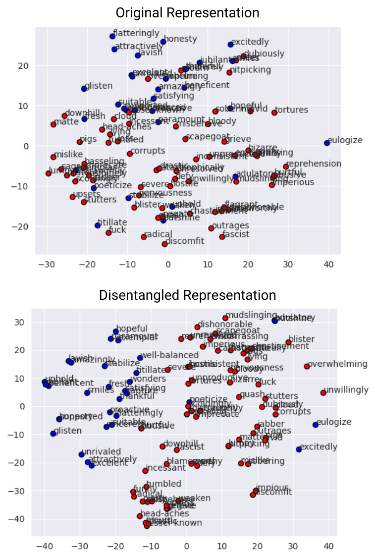
Figure 1: A subset of 100 word vectors from an opinion lexicon (Hu & Liu, 2004). We trained an autoencoder network for 50 epochs to learn a disentangled latent code representation for an opinion lexicon. We can see the disentangled word vectors for positive and negative words denoted by colors blue and red respectively. In the transformed representation, we can see a better clustering of the positive and negative words respectively. This figure is best viewed in color.

2.4 Soft Nearest Neighbor Loss

In the context of our work, we define disentanglement as how close pairs of class-similar feature representations are, relative to pairs of class-different feature representations. Frosst et al. used the same term in the same context. A low entanglement value implies that feature representations from the same class are closer together than they are to feature representations from different classes. To measure the entanglement of feature representations, Frosst et al. expanded the non-linear neighborhood component analysis (NCA) (Salakhutdinov & Hinton, 2007) objective by introducing the temperature factor $T$, and called this modified objective the soft nearest neighbor loss.
They defined the soft nearest neighbor loss as the non-linear NCA at temperature $T$, for a batch of $b$ samples $(x,y)$,

$$\ell_{snn}(x,y,T)=-\dfrac{1}{b}\sum_{i\in 1\dots b}\log\left(\dfrac{\sum\limits_{\begin{subarray}{c}j\in 1\dots b\\ j\neq i\\ y_{i}=y_{j}\end{subarray}}\exp\left(-\dfrac{d_{ij}}{T}\right)}{\sum\limits_{\begin{subarray}{c}k\in 1\dots b\\ k\neq i\end{subarray}}\exp\left(-\dfrac{d_{ik}}{T}\right)}\right)$$ (4)

where $d$ is a distance metric on either raw input features or learned hidden layer representations $x$ of a neural network, and $T$ is the temperature factor that is directly proportional to the distances among the data points. We use the pairwise cosine distance (see Eq. 5) as our distance metric on all our experiments for more stable computations.

$$d_{ij}=1-\dfrac{\sum_{n}^{N}x_{i}x_{j}}{\sqrt{\sum_{n}^{N}x_{i}^{2}}\sqrt{\sum_{n}^{N}x_{j}^{2}}}$$ (5)

Similarly, we employ the annealing temperature (see Eq. 6) proposed by Agarap & Azcarraga for more stable computations.

$$T=\dfrac{1}{(\eta+i)^{\gamma}}$$ (6)

where $i$ is the current training epoch index, and we set $\eta=1$ and $\gamma=0.55$ for our experiments, similar to Neelakantan et al..

Frosst et al. described the temperature factor as a means to control the relative importance of the distances between pairs of points, that is, the loss is dominated by small distances when using a low temperature. We can describe the soft nearest neighbor loss as the negative log probability of sampling a neighboring data point $j$ from the same class as $i$ in a mini-batch $b$, which is similar to the probabilistic sampling by Goldberger et al.. A low soft nearest neighbor loss value is implies a low entanglement (or high disentanglement).
In Figure 1, we show a disentangled latent code representation for the word vectors from an opinion lexicon by (Hu & Liu, 2004). In the aforementioned figure, we can see a better separation of the word vectors from the two classes.

3 Downstream Tasks on Disentangled Representations

We demonstrate the effectiveness of our approach by conducting experiments on a benchmark dataset, and lay down the classification and clustering performance of our baseline and experimental models.

3.1 Dataset

Due to time and computational restraints, we were only able to run experiments on one dataset. In future works, we intend to use more datasets. In the current study, we use the AG News dataset, a text classification dataset that is comprised of four classes (Zhang et al., 2015). Despite the training set having a 119,843 documents, we only use a subset of it in select experiments due to time and computational resource constraints. However, we still used the full test set of 7,600 documents for our evaluations. We removed the English stop words, the words that have less than 3 characters, and the non-alphanumeric characters. Then, we normalized the texts into lowercase.
We computed the sentence embeddings before training to save time and computation resources. For the first set of sentence embeddings, we computed the average GloVe (Pennington et al., 2014) word embeddings for each example using SpaCy (Honnibal & Montani, 2017), while for the second set of sentence embeddings, we computed the InferSent embeddings for each example.
Our first set of sentence embeddings had 300 dimensions for each example, while the second set of embeddings had 4096 dimensions for each example. The large gap between the dimensionalities of the sentence embeddings we used was due to the use of bidirectional RNN-LSTM in InferSent.

3.2 Experimental Setup

We used a computing machine with Intel Core i5-6300 HQ (2.60 GHz) with 16 GB DDR3 RAM and Nvidia GTX 960M 4GB GDDR5 GPU. We ran our computations for each of our experiments for five times, each of which used a pseudorandom seed for reproducibility. The seeds we used were as follows: 42, 1234, 73, 1024, and 31415926.
For our experiments where we used the averaged word embeddings as the sentence embeddings, we only used a pseudorandomly picked subset with 20,000 examples while we still used the full test with 7,600 examples for evaluation. As for our experiments where we used the InferSent embeddings as the sentence embeddings, we used the full training set with 119,843 examples and the full test with 7,600 examples for evaluation.

3.3 Text Classification

We trained feed-forward neural networks and and convolutional neural networks using a composite loss (see Eq. 7) of the cross entropy as the classification loss, and the soft nearest neighbor loss as the regularizer.

$$\mathcal{L}(f,x,y)=\ell_{ce}\left(y,f(x)\right)+\alpha\cdot\sum_{b\in B}\ell_{snn}\left(f^{(b)}(x),y\right)$$ (7)

where $b$ is the index of the hidden layer of the neural network. We did not perform any hyperparameter turning or any training tricks since we only want to show that we can use disentanglement for some natural language processing tasks. Our neural networks were trained using Adam (Kingma & Ba, 2014) optimization with a learning rate of $1\times 10^{-3}$ on a mini-batch size of 256 for 30 epochs for the feed-forward neural networks and 50 epochs for the convolutional neural networks. We used an $\alpha$ value of 100 for disentanglement and -100 for entanglement. The rationale for entanglement is based on the findings by Frosst et al., where they showed that entangling the representations in the hidden layer of a network results to an even better disentanglement in the classification layer.

Model	SpaCy Embeddings				InferSent Embeddings
	ACC		F1		ACC		F1
	AVG	MAX	AVG	MAX	AVG	MAX	AVG	MAX
Baseline	87.31%	88.18%	0.8732	0.8818	89.34%	89.74%	0.8934	0.8974
SNNL 100	88.02%	88.22%	0.8802	0.8822	89.58%	89.68%	0.8958	0.8968
SNNL -100	81.71%	82.71%	0.8109	0.8271	89.60%	90.11%	0.8960	0.9011

Table 1: Using a composite loss, which minimizes cross entropy loss and optimizes entanglement through the soft nearest neighbor loss, has a marginal increase in test performance on the AG News dataset classification using a feed-forward neural network.

Model	SpaCy Embeddings				InferSent Embeddings
	ACC		F1		ACC		F1
	AVG	MAX	AVG	MAX	AVG	MAX	AVG	MAX
Baseline	87.08%	87.42%	0.8708	0.8742	86.92%	88.42%	0.8692	0.8842
SNNL 100	87.19%	87.89%	0.8719	0.8789	87.67%	88.74%	0.8767	0.8874
SNNL -100	49.98%	75.82%	0.4998	0.7582	25%	25%	0.25	0.25

Table 2: Using a composite loss, which minimizes cross entropy loss and optimizes entanglement through the soft nearest neighbor loss, has a marginal increase in test performance on the AG News dataset classification using a convolutional neural network.

In Tables 1 and 2, we can see marginal improvement in the test classification performance of our experimental model. In Table 1, we can see the test classification performance of our feed-forward neural network on the averaged GloVe word embeddings as the sentence embeddings. Through disentanglement, our network performs better than the baseline model but performs worse through entanglement. We may attribute this to our use of relatively shallow neural networks, i.e. having two hidden layers at most, while the models in (Frosst et al., 2019) were much deeper, e.g. having five hidden layers at the minimum. We posit that entanglement or disentanglement works even better with deeper models. However, on the InferSent embeddings, we see a marginal increase in test classification performance when using entanglement. In Table 2, we see a consistent performance by our convolutional neural network when disentangling hidden layer representations, outperforming the baseline and entanglement models.

3.4 Text Clustering

We trained an autoencoder network using a composite loss (see Eq. 8) of the binary cross entropy as the reconstruction loss, and the soft nearest neighbor loss as the regularizer.

$$\mathcal{L}(f,x,y)=\ell_{rec}\left(x,f(x)\right)+\alpha\cdot\sum_{b\in B}\ell_{snn}\left(f^{(b)}(x),y\right)$$ (8)

Similar to our classification experiments, we did not perform any hyperparameter tuning or any training tricks. Our autoencoder was trained using Adam optimization with a learning rate of $1\times 10^{-3}$ on a mini-batch size of 256 for 30 epochs. Unlike the classification experiments, we only used an $\alpha$ value of 100 due to time constraints. For autoencoding, we had two modes of disentanglement: the first is by disentangling only a part of the latent code, particularly, only 100 of its 128 units à la (Salakhutdinov & Hinton, 2007), and the second is by disentangling all the hidden layers of the autoencoder network.
Afterwards, we use the disentangled latent code, from these two modes of disentanglement, as the input features for our k-Means clustering algorithm (Lloyd, 1982).

We used the number of ground-truth categories in our dataset as the number of clusters. We used six different metrics to evaluate the clustering performance of our baseline and experimental models. The first three metrics fall under the category of internal criteria for clustering evaluation, which measure clustering quality. The second three metrics fall under the category of external criteria for clustering evaluation, which measure clustering membership.

3.4.1 Internal Criteria

In internal criteria for clustering evaluation, the clustering is subjected to optimizing the intra- and inter-cluster similarity. Specifically, to obtain a high intra-cluster similarity, and a low inter-cluster similarity. These optimization metrics are based on the cluster quality alone, without any external validation. We note that good scores in internal criteria metrics may not necessarily imply the effectiveness of the clustering model.

3.4.1.1    Davies-Bouldin Index

(DBI) is the ratio between the intra-cluster distances and the inter-cluster distances (Davies & Bouldin, 1979; Halkidi et al., 2001). A low DBI denotes a good cluster separation. We compute it using Eq. 9,

$$DBI=\dfrac{1}{k}\sum_{i=1}^{k}\max_{i\neq j}R_{j}$$ (9)

where $R$ is the mean similarity among clusters given by the following equation,

$$R_{ij}=\dfrac{s_{i}+s_{j}}{d_{ij}}$$ (10)

where $s$ is the cluster diameter which is the average distance between each point in the cluster and the cluster centroid, and $d_{ij}$ is the distance between centroids $i$ and $j$.

3.4.1.2    Silhouette Score

(SIL) measures the similarity among examples in their own cluster compared to other clusters (Rousseeuw, 1987), and we compute it using Eq. 11,

$$SIL=\dfrac{b(i)-a(i)}{\max\left[a(i),b(i)\right]}$$ (11)

where $a(i)$ is the average within-cluster distances, and we compute it using the following equation,

$$a(i)=\dfrac{1}{|C_{i}|-1}\sum_{j\in C_{i},i\neq j}d(i,j)$$ (12)

where $C_{i}$ is the predicted cluster for point $i$, and $d(i,j)$ is the distance between points $i$ and $j$. Then, $b(i)$ is the average nearest-cluster distance, and we compute it using the following equation, 13,

$$b(i)=\min_{k\neq i}\dfrac{1}{|C_{k}|}\sum_{j\in C_{k}}d(i,j)$$ (13)

Although any distance metric may be used, we used the Euclidean distance for our evaluations.

3.4.1.3    Calinski-Harabasz Score

(CHS) is the ratio of intra-cluster dispersion to inter-cluster dispersion, and we compute it using Eq. 14. A high CHS denotes good cluster separation (Caliński & Harabasz, 1974).

$$CHS=\dfrac{Tr(B_{k})}{Tr(W_{k})}\times\dfrac{N-k}{k-1}$$ (14)

where $B_{k}$ is the inter-cluster dispersion matrix given by the following,

$$B_{k}=\sum_{q}n_{q}(c_{q}-c)(c_{q}-c)^{T}$$ (15)

and $W_{k}$ is the intra-cluster dispersion matrix given by the following,

$$W_{k}=\sum_{q=1}^{k}\sum_{x\in C_{q}}(x-c_{q})(x-c_{q})^{T}$$ (16)

where $N$ is the number of points in the data, $C_{q}$ contains the data of points in cluster $q$, $c_{q}$ is the center of cluster $q$, $c$ is the center of $C$, and $n_{q}$ is the number of data points in cluster $q$.

3.4.2 External Criteria

In external criteria for clustering evaluation, we use external information such as the class labels of a benchmark dataset for our validation. The external criteria metrics measure the clustering membership of the data points by using the class labels as the pseudo-cluster labels. Using the ground-truth labels as the pseudo-cluster labels is based on the cluster assumption in the semi-supervised learning literature (Chapelle et al., 2009).

3.4.2.1    Normalized Mutual Information

(NMI) is the normalization of the mutual information (MI) score to transform its value to the $[0,1]\in\mathbb{R}$ range, where 0 implies no mutual information while 1 implies perfect correlation. We compute it using the following,

$$NMI=\dfrac{2I(y,c)}{[H(y)+H(c)]}$$ (17)

where $y$ is the pseudo-cluster label, $c$ is the predicted cluster label, $H$ is the entropy, and $I$ is the mutual information between the pseudo-cluster labels and the predicted cluster labels.

3.4.2.2    Adjusted Rand Index

(ARI) is the Rand Index (RI) adjusted for chance (Hubert & Arabie, 1985). It measures the similarity between two clusterings by iterating through all pairs of points and counting pairs assigned to the same or different clusters according to the pseudo-cluster labels and the predicted cluster labels (see Eq. 18).

$$RI=\dfrac{TP+TN}{TP+FP+FN+TN}$$ (18)

where $TP$ is the true positive, $TN$ is the true negative, $FP$ is the false positive, and $FN$ is the false negative. We then compute ARI from RI through the following,

$$ARI=\dfrac{RI-\mathbb{E}[RI]}{\max(RI)-\mathbb{E}[RI]}$$ (19)

ARI values are in $[0,1]\in\mathbb{R}$ range, where 0 implies random labelling independently of the number of clusters, while 1 implies the clusterings are identical up to a permutation.

3.4.2.3    Clustering Accuracy

(ACC) is the best match between the pseudo-cluster labels and the predicted clusters (Yang et al., 2010).

$$ACC=\max_{m}\dfrac{\sum\limits_{i=1}^{n}1\{l_{i}=m\left(c_{i}\right)\}}{n},$$ (20)

where $l_{i}$ is the pseudo-cluster label, $c_{i}$ is the predicted cluster label, and $m$ ranges over all possible one-to-one mappings between the labels and the clusters.

Model	SpaCy Embeddings						InferSent Embeddings
	DBI		SIL		CHS		DBI		SIL		CHS
	AVG	MIN	AVG	MAX	AVG	MAX	AVG	MIN	AVG	MAX	AVG	MAX
Orig.	2.72	2.72	0.10	0.10	684.14	684.32	2.85	2.85	0.092	0.092	592.55	592.77
AE	2.18	0	0.28	1	207846.94	1036948.01	1.88	1.30	0.68	0.99	675.47	1315.52
LC(D)	0.71	0.59	0.55	0.59	11291.57	15142.86	0.70	0.56	0.61	0.64	11092.32	12723.00
AE(D)	0.38	0.34	0.76	0.79	24172.28	27989.27	0.60	0.52	0.67	0.70	12275.96	13767.69

Table 3: Using a composite loss, which minimizes binary cross entropy loss and minimizes entanglement through soft nearest neighbor loss, has a significant increase in clustering quality on the AG News dataset using an autoencoder network.

Model	SpaCy Embeddings						InferSent Embeddings
	NMI		ARI		ACC		NMI		ARI		ACC
	AVG	MAX	AVG	MAX	AVG	MAX	AVG	MAX	AVG	MAX	AVG	MAX
Orig.	0.51	0.51	0.52	0.52	0.78	0.79	0.53	0.53	0.57	0.57	0.81	0.81
AE	0.44	0.57	0.46	0.61	0.70	0.83	0.06	0.28	0.04	0.19	0.30	0.49
LC(D)	0.67	0.68	0.71	0.72	0.88	0.88	0.64	0.66	0.66	0.70	0.86	0.88
AE(D)	0.68	0.68	0.72	0.72	0.88	0.89	0.65	0.67	0.67	0.71	0.86	0.88

Table 4: Using a composite loss, which minimizes binary cross entropy loss and minimizes entanglement through soft nearest neighbor loss, has a significant increase in clustering membership performance on the AG News dataset using an autoencoder network.

3.5 Clustering Performance Evaluation

Since autoencoder and clustering are unsupervised learning techniques, we simulate the lack of labelled datasets by using only a subset of 10,000 labelled examples for training our InferSent models while we still use the 20,000 labelled examples for training our SpaCy models. For our baseline models, we encode the original feature representation (which we denote by “Orig.”) using principal components analysis to 128 dimensions (the same dimensionality used by our autoencoders), and we use the latent code representation from our baseline autoencoder. The resulting lower-dimensional representation of our sentence embeddings are the inputs to our k-Means clustering model.
In Table 3, we can see that encoding the sentence embeddings using an autoencoder network improves the clustering quality of the learned representations. When using the averaged word embeddings, we can see that our autoencoder with disentangled hidden layers outperformed all the models in terms of DBI and SIL on average over our five runs, but lost significantly in terms of CHS due to one of the runs (seed 31415926) on the baseline autoencoder had 1,036,948.01 as its CHS (and DBI of 0 and SIL of 1). However, if we exclude the baseline autoencoder run on seed 31415926, it has only 571.67 as its CHS. But when using the InferSent embeddings, we see a more consistent result of our experimental models outperforming our baseline models, and only losing to our baseline autoencoder by a slim margin in terms of SIL.
In Table 4, we see a significant clustering membership improvement when using disentangled representations for clustering. Surprisingly, even without any ground-truth information unlike our experimental models, the baseline autoencoder performed well when using the averaged word embeddings. Similarly, we have a decent baseline performance as well on the original feature representation for both the averaged word embeddings and InferSent embeddings. For the latter, we cite Cover’s theorem which states that by transforming a non-linearly separable data into higher-dimensional space, we can obtain a linearly separable representation of the data, noting that the averaged word embeddings and InferSent embeddings had 300 and 4096 dimensions respectively at the begining, and only transformed to 128 dimensions by using PCA. Furthermore, this even supports the study by Wieting & Kiela, where their random encoders performed on par with the models in (Conneau et al., 2017), suggesting that the sentence encoding in 4096 dimensions takes the most credit for rendering the classification task easier. As for our experimental models, both disentangling the latent code layer and all the hidden layers of the autoencoder improved the clustering performance in terms of cluster membership as indicated by their high NMI, ARI, and ACC scores.

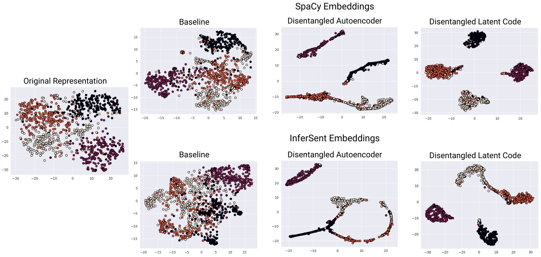
Figure 2: Visualization comparing the original representation with the learned latent code representations by the baseline autoencoder, our autoencoder with disentangled hidden layers, and our autoencoder with disentangled latent code layer. To achieve this visualization, the representations were encoded using t-SNE (Maaten & Hinton, 2008) with perplexity = 50.0 and learning rate = 200.0, optimized for 1,000 iterations, using the same random seed for all the computations. This figure is best viewed in color.

3.6 Visualizing Disentangled Text Representations

We show the latent code representations for both the averaged GloVe embeddings and the InferSent embeddings using our baseline autoencoder, autoencoder with disentangled hidden layers, and autoencoder with disentangled latent code layer in Figure 2, together with the original InferSent embeddings representation. We obtain these latent code representations from our clustering experiments. Visually, we can confirm that with disentanglement, we were able to have better-defined clusters.

4 Conclusion and Future Directions

To the best of our knowledge, this is the first work on disentangling natural language representations for classification and clustering since the seminal papers on soft nearest neighbor loss focused on image classification and image generation tasks (Frosst et al., 2019; Goldberger et al., 2005; Salakhutdinov & Hinton, 2007). Our experimental models consistently outperformed our baseline models with marginal improvement on text classification and significant improvement on text clustering, both in the form of sentence embeddings. Moreoever, our findings show that there is only a marginal improvement in performance when using actual sentence embeddings over an averaged word embeddings. We aim to apply disentanglement on more natural language processing tasks such as langauge generation, sentiment analysis, and word embeddings analysis. We also aim to use more datasets for a stronger set of empirical results.

References

- Agarap & Azcarraga (2020) Agarap, A. F. and Azcarraga, A. P. Improving k-means clustering performance with disentangled internal representations. arXiv preprint arXiv:2006.04535, 2020.
- Arora et al. (2016) Arora, S., Liang, Y., and Ma, T. A simple but tough-to-beat baseline for sentence embeddings. 2016.
- Bengio et al. (2013) Bengio, Y., Courville, A., and Vincent, P. Representation learning: A review and new perspectives. IEEE transactions on pattern analysis and machine intelligence, 35(8):1798–1828, 2013.
- Bourlard & Kamp (1988) Bourlard, H. and Kamp, Y. Auto-association by multilayer perceptrons and singular value decomposition. Biological cybernetics, 59(4-5):291–294, 1988.
- Caliński & Harabasz (1974) Caliński, T. and Harabasz, J. A dendrite method for cluster analysis. Communications in Statistics-theory and Methods, 3(1):1–27, 1974.
- Chapelle et al. (2009) Chapelle, O., Scholkopf, B., and Zien, A. Semi-supervised learning (chapelle, o. et al., eds.; 2006)[book reviews]. IEEE Transactions on Neural Networks, 20(3):542–542, 2009.
- Conneau et al. (2017) Conneau, A., Kiela, D., Schwenk, H., Barrault, L., and Bordes, A. Supervised learning of universal sentence representations from natural language inference data. arXiv preprint arXiv:1705.02364, 2017.
- Davies & Bouldin (1979) Davies, D. L. and Bouldin, D. W. A cluster separation measure. IEEE transactions on pattern analysis and machine intelligence, (2):224–227, 1979.
- Devlin et al. (2018) Devlin, J., Chang, M.-W., Lee, K., and Toutanova, K. Bert: Pre-training of deep bidirectional transformers for language understanding. arXiv preprint arXiv:1810.04805, 2018.
- Frosst et al. (2019) Frosst, N., Papernot, N., and Hinton, G. Analyzing and improving representations with the soft nearest neighbor loss. arXiv preprint arXiv:1902.01889, 2019.
- Goldberger et al. (2005) Goldberger, J., Hinton, G. E., Roweis, S. T., and Salakhutdinov, R. R. Neighbourhood components analysis. In Advances in neural information processing systems, pp. 513–520, 2005.
- Halkidi et al. (2001) Halkidi, M., Batistakis, Y., and Vazirgiannis, M. On clustering validation techniques. Journal of intelligent information systems, 17(2-3):107–145, 2001.
- He et al. (2015) He, K., Zhang, X., Ren, S., and Sun, J. Delving deep into rectifiers: Surpassing human-level performance on imagenet classification. In Proceedings of the IEEE international conference on computer vision, pp. 1026–1034, 2015.
- Hinton & Salakhutdinov (2006) Hinton, G. E. and Salakhutdinov, R. R. Reducing the dimensionality of data with neural networks. science, 313(5786):504–507, 2006.
- Hinton & Zemel (1994) Hinton, G. E. and Zemel, R. S. Autoencoders, minimum description length and helmholtz free energy. In Advances in neural information processing systems, pp. 3–10, 1994.
- Hochreiter & Schmidhuber (1997) Hochreiter, S. and Schmidhuber, J. Long short-term memory. Neural computation, 9(8):1735–1780, 1997.
- Honnibal & Montani (2017) Honnibal, M. and Montani, I. spacy 2: Natural language understanding with bloom embeddings, convolutional neural networks and incremental parsing. To appear, 7(1), 2017.
- Hu & Liu (2004) Hu, M. and Liu, B. Mining and summarizing customer reviews. In Proceedings of the tenth ACM SIGKDD international conference on Knowledge discovery and data mining, pp. 168–177, 2004.
- Hubert & Arabie (1985) Hubert, L. and Arabie, P. Comparing partitions. Journal of classification, 2(1):193–218, 1985.
- Joulin et al. (2016) Joulin, A., Grave, E., Bojanowski, P., Douze, M., Jégou, H., and Mikolov, T. Fasttext. zip: Compressing text classification models. arXiv preprint arXiv:1612.03651, 2016.
- Kingma & Ba (2014) Kingma, D. P. and Ba, J. Adam: A method for stochastic optimization. arXiv preprint arXiv:1412.6980, 2014.
- LeCun et al. (1998) LeCun, Y., Bottou, L., Bengio, Y., and Haffner, P. Gradient-based learning applied to document recognition. Proceedings of the IEEE, 86(11):2278–2324, 1998.
- Lloyd (1982) Lloyd, S. Least squares quantization in pcm. IEEE transactions on information theory, 28(2):129–137, 1982.
- Maaten & Hinton (2008) Maaten, L. v. d. and Hinton, G. Visualizing data using t-sne. Journal of machine learning research, 9(Nov):2579–2605, 2008.
- Mikolov et al. (2013) Mikolov, T., Sutskever, I., Chen, K., Corrado, G. S., and Dean, J. Distributed representations of words and phrases and their compositionality. In Advances in neural information processing systems, pp. 3111–3119, 2013.
- Mikolov et al. (2018) Mikolov, T., Grave, E., Bojanowski, P., Puhrsch, C., and Joulin, A. Advances in pre-training distributed word representations. In Proceedings of the International Conference on Language Resources and Evaluation (LREC 2018), 2018.
- Nair & Hinton (2010) Nair, V. and Hinton, G. E. Rectified linear units improve restricted boltzmann machines. In ICML, 2010.
- Neelakantan et al. (2015) Neelakantan, A., Vilnis, L., Le, Q. V., Sutskever, I., Kaiser, L., Kurach, K., and Martens, J. Adding gradient noise improves learning for very deep networks. arXiv preprint arXiv:1511.06807, 2015.
- Pennington et al. (2014) Pennington, J., Socher, R., and Manning, C. D. Glove: Global vectors for word representation. In Proceedings of the 2014 conference on empirical methods in natural language processing (EMNLP), pp. 1532–1543, 2014.
- Peters et al. (2018) Peters, M. E., Neumann, M., Iyyer, M., Gardner, M., Clark, C., Lee, K., and Zettlemoyer, L. Deep contextualized word representations. arXiv preprint arXiv:1802.05365, 2018.
- Rousseeuw (1987) Rousseeuw, P. J. Silhouettes: a graphical aid to the interpretation and validation of cluster analysis. Journal of computational and applied mathematics, 20:53–65, 1987.
- Rumelhart et al. (1985) Rumelhart, D. E., Hinton, G. E., and Williams, R. J. Learning internal representations by error propagation. Technical report, California Univ San Diego La Jolla Inst for Cognitive Science, 1985.
- Salakhutdinov & Hinton (2007) Salakhutdinov, R. and Hinton, G. Learning a nonlinear embedding by preserving class neighbourhood structure. In Artificial Intelligence and Statistics, pp. 412–419, 2007.
- Vincent et al. (2008) Vincent, P., Larochelle, H., Bengio, Y., and Manzagol, P.-A. Extracting and composing robust features with denoising autoencoders. In Proceedings of the 25th international conference on Machine learning, pp. 1096–1103, 2008.
- Vincent et al. (2010) Vincent, P., Larochelle, H., Lajoie, I., Bengio, Y., Manzagol, P.-A., and Bottou, L. Stacked denoising autoencoders: Learning useful representations in a deep network with a local denoising criterion. Journal of machine learning research, 11(12), 2010.
- Wieting & Kiela (2019) Wieting, J. and Kiela, D. No training required: Exploring random encoders for sentence classification. arXiv preprint arXiv:1901.10444, 2019.
- Yang et al. (2010) Yang, Y., Xu, D., Nie, F., Yan, S., and Zhuang, Y. Image clustering using local discriminant models and global integration. IEEE Transactions on Image Processing, 19(10):2761–2773, 2010.
- Zhang et al. (2015) Zhang, X., Zhao, J., and LeCun, Y. Character-level convolutional networks for text classification. In Advances in neural information processing systems, pp. 649–657, 2015.