Distribution free optimality intervals for clustering

Abstract

We address the problem of validating the ouput of clustering algorithms. Given data ${\cal D}$ and a partition ${\cal C}$ of these data into $K$ clusters, when can we say that the clusters obtained are correct or meaningful for the data? This paper introduces a paradigm in which a clustering ${\cal C}$ is considered meaningful if it is good with respect to a loss function such as the K-means distortion, and stable, i.e. the only good clustering up to small perturbations. Furthermore, we present a generic method to obtain post-inference guarantees of near-optimality and stability for a clustering ${\cal C}$. The method can be instantiated for a variety of clustering criteria (also called loss functions) for which convex relaxations exist. Obtaining the guarantees amounts to solving a convex optimization problem. We demonstrate the practical relevance of this method by obtaining guarantees for the K-means and the Normalized Cut clustering criteria on realistic data sets. We also prove that asymptotic instability implies finite sample instability w.h.p., allowing inferences about the population clusterability from a sample. The guarantees do not depend on any distributional assumptions, but they depend on the data set ${\cal D}$ admitting a stable clustering. Keywords: clustering, convex optimization, distribution free, K-means, loss-based clustering, Normalized Cut, stability

1 Introduction

We are concerned with the problem of finding structure in data by clustering. This is an old problem, yet some of the most interesting advances in its theoretical understanding are recent. Namely, while empirical evidence has been suggesting that when the data are “well clustered”, the cluster structure is easy to find, proving this in the non-asymptotic regime is an area of current progress. For instance, it was shown that finding an almost optimal clustering for the K-means and K-medians cost can be done by efficient algorithms when clusters are “well separated” Awasthi et al., 2015a , or when the optimal clustering is “resilient” balcanL:16. These results are significant because they promise computationally efficient inference in the special case when the data are “clusterable”, even though most clustering loss functions induce hard optimization problems in the worst case.

The present paper addresses the post-inference aspect of clustering. We propose a framework for providing guarantees for a given clustering ${\cal C}$ of a given set of points, without making untestable assumptions about the data generating process. In the simplest terms, the question we address is: can a user tell, with no prior knowledge, if the clustering ${\cal C}$ returned by a clustering algorithm is meaningful? or correct? or optimal?

This is the fundamental problem of cluster validation, and we call it Distribution Free Cluster Validation (DFCV). We offer a general data driven DFCV paradigm, in the case of loss-based clustering. In this framework, for a given number of clusters $K$, the best clustering of the data is the one that minimizes a loss function $\operatorname{Loss}({\cal D},{\cal C})$. This framework includes K-means, K-medians, graph partitioning, etc. Note that these loss functions as well as most clustering losses in use are NP-hard to optimize  Garey and Johnson, (1979). In particular, this means that it is in general not possible to prove that the optimum has been found Garey and Johnson, (1979). Thus, the DFCV problem needs to be carefully framed before solving it is attempted.

This paper will show that it is possible to obtain a guarantee of “correctness” for a clustering precisely in those cases when the data at hand admits a good clustering; in other words, when the data is “clusterable”.

1.1 Framing the problem.

The loss as goodness of fit How, thus, do we decide if ${\cal C}$ is a “meaningful” clustering for data ${\cal D}$? First, ${\cal C}$ must be “good” with respect to whatever definition of clustering we are working with. This definition is embodied by the loss function $\operatorname{Loss}$. For example, in the case of K-means clustering, the loss function $\operatorname{Loss}_{\rm Km}$ is the quadratic distortion defined in equation (7), and in the case of graph partitioning by Normalized Cuts Meilă and Shi, 2001b the loss function $\operatorname{Loss}_{\rm NCut}$ is defined in equation (14). Only a clustering ${\cal C}$ that has low loss can be considered meaningful; indeed, if the value of $\operatorname{Loss}({\cal C})$ was much larger than the loss for other ways of grouping the data, ${\cal C}$ could not be a good or meaningful way to partition the data according to the user’s definition of clustering. Hence, the proposed DFCV framework the $\operatorname{Loss}$ is a precise way to express what a user means by “cluster” from the multitude of definitions possible.

Stability (uniqueness) Second, ${\cal C}$ must be the only “good” clustering supported by the data ${\cal D}$, up to small variations. This property is called stability. In the present paper results of the following form will be obtained.

Stability Theorem ($*$)

Given a clustering ${\cal C}$ of data set ${\cal D}$, a loss function $\operatorname{Loss}()$, and technical conditions ${\mathcal{T}}$, there is an $\epsilon$ such that $d^{EM}({\cal C},{\cal C}^{\prime})\leq\epsilon$ whenever $\operatorname{Loss}({\cal D},{\cal C}^{\prime})\leq\operatorname{Loss}({\cal D},{\cal C})$.

In the above $d^{EM}({\cal C},{\cal C}^{\prime})$ is the widely used earth mover’s distance (EM) distance between partitions of a set of $n$ objects, formally defined in Section 2. Theorem $*$ would be trivial if $\epsilon$ was arbitrarily large; hence, we shall always require that $\epsilon$ be small, for instance, smaller than the relative size of the smallest cluster in ${\cal C}$.

A Stability Theorem states that any way to partition the data which is very different from ${\cal C}$ will result in higher cost. Hence, the data supports only one way to be partitioned with low cost, and small perturbations thereof. If a statement such as $(*)$ holds for a clustering ${\cal C}$, it means that ${\cal C}$ captures structure existing in the data, thus it is meaningful. It should also be evident that it is not possible to obtain such guarantees in general; they can only exist for specific data sets and clusterings, as illustrated in Figure 1. A clustering satisfying the Stability Theorem is called $\epsilon$-stable (or simply stable), and a data set that admits an $\epsilon$-stable clustering is said to be $\epsilon$-clusterable (or simply clusterable).

From Theorem $(*)$ it follows immediately that $C^{{\rm opt}}$, the clustering minimizing $\operatorname{Loss}$ on ${\cal D}$, together with the entire sublevel set $\{{\cal C}^{\prime},\,\operatorname{Loss}({\cal C}^{\prime})\leq\operatorname{Loss}({\cal C})\}$ is contained in the ball of radius $\epsilon$ centered at ${\cal C}$. We call this ball an optimality interval (OI) for $\operatorname{Loss}$ on ${\cal D}$. Somehow abusively, we will occasionally call $\epsilon$ itself an OI.

It is important that the conditions of the Stability Theorem and the value of $\epsilon$ above be computable from ${\cal D}$ and ${\cal C}$. That is, they must be tractable to evaluate, and must not contain undefined constants. Figure 1 illustrates this framework.

To summarize, the Distribution Free Cluster Validation framework starts with a loss function $\operatorname{Loss}({\cal D},{\cal C})$ which serves both as clustering paradigm, by defining implicitly the type of clusters appropriate for the application, and as goodness of fit measure. Supposing that it is possible to find a good clustering ${\cal C}$, the challenge is to verify that ${\cal C}$ is stable without enumerating all the other possible $K$-partitions of the data. Hence, the main technical contribution of this work is to show how to obtain conditions ${\mathcal{T}}$ that can be verified tractably. The key idea is to uses convex tractable relaxations to the original $\operatorname{Loss}$ minimization problem.

After the definitions in Section 2, in Section 3 we introduce the Sublevel Set (SS) method, a generic method for obtaining technical conditions ${\mathcal{T}}$, stability theorems such as ($*$) and optimality intervals for loss-based clustering, from tractable convex relaxations. We will illustrate the working of this method for the K-means cost function (Sections 3.1 and 6.1), for graph partitioning by Normalized Cuts (Sections 3.2 and 6.2), to any of a large class of losses (Section 3.3). Section 4 defines stability in the population setting. The relationship with previous work is presented in Section 5, and the discussion in Section 7 concludes the paper.

Good, stable ${\cal C}$	Bad ${\cal C}^{\prime}$	Unstable ${\cal C}^{\prime\prime}$
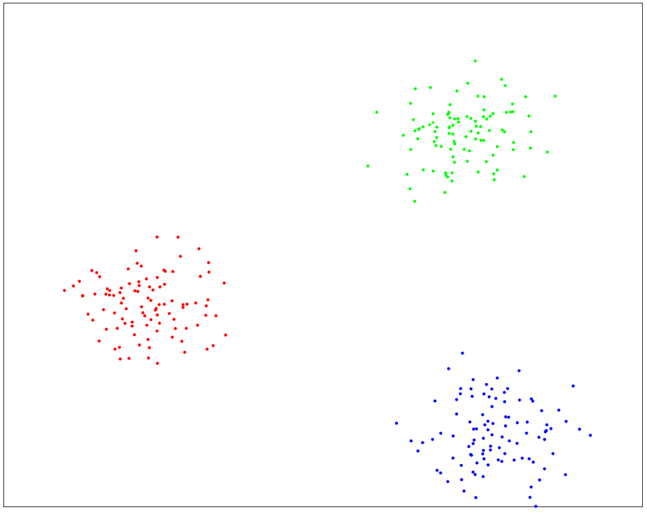
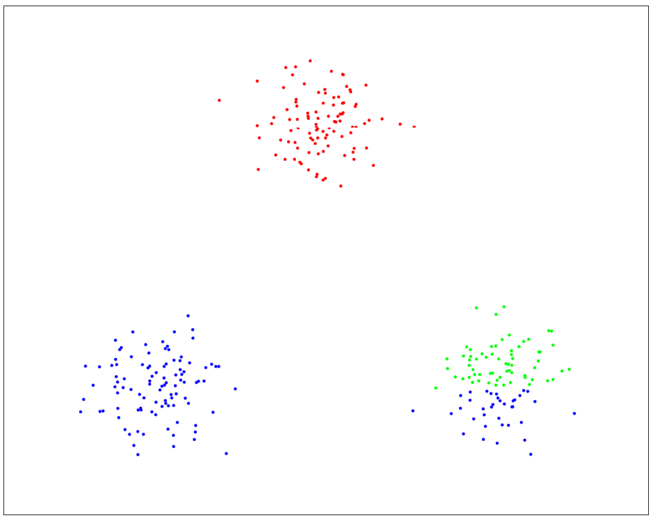
OI $\epsilon=10^{-4}$	no guarantee	no guarantee

Figure 1: Left: a clusterable data set. The method described in Section 3.1 guarantees than all clusterings of this data set that are at least as “good” as ${\cal C}$ differ from it in no more $\epsilon=0.01\%$ of the points; since $\epsilon<1/n$, this guarantee also implies that ${\cal C}$ is optimal w.r.t. $\operatorname{Loss}$. Middle: the same data, with a clustering ${\cal C}^{\prime}$ which is neither good, nor stable. Right: a data set that is not clusterable. The clustering shown is nearly optimal, but it is not stable, as the data admits other clusterings with similar $\operatorname{Loss}$, but very different from ${\cal C}^{\prime\prime}$.

2 Preliminaries and definitions

Representing clusterings as matrices

Let ${\cal D}=\{x_{1},\ldots x_{n}\}$ be the data to be clustered. We make no assumptions about the distribution of these data for now. A clustering ${\cal C}=\{C_{1},\ldots\,C_{K}\}$ of the data set ${\cal D}$ is a partition of the indices $\{1,2,\ldots n\}\stackrel{{\scriptstyle def}}{{=}}[n]$ into $K$ non-empty mutually disjoint subsets $C_{1},\ldots C_{K}$, called clusters. We denote by $\mathbf{{C}}_{K}$ the space of all clusterings with $K$ clusters.

Let $n_{k}=|C_{k}|$ for $k=1,\ldots K$, with $\sum_{k=1}^{K}n_{k}=n$; further, let $p_{\rm min}=\min_{k\in[K]}n_{k}/n,\,p_{\rm max}=\max_{k\in[K]}n_{k}/n$ represent the minimum, respectively maximum relative cluster sizes.

A clustering ${\cal C}$ can be represented by an $n\times n$ clustering matrix $X$ defined as

$$X\;=\;[X_{ij}]_{i,j=1}^{n},\quad X_{ij}\;=\;\left\{\begin{array}[]{ll}1/{n_{k}}&\text{if }i,j\in C_{k}\,\text{for some $k\in[K]$}\\ 0&\text{otherwise.}\\ \end{array}\right.$$ (1)

The following proposition lists the properties of the matrix $X$. The proof (which is straightforward) can be found in the Appendix, along with all other proofs.

Proposition 1

For any clustering ${\cal C}$ of $n$ data points, the matrix $X$ defined by (1) has elements $X_{ij}$ in $[0,1]$; $\operatorname{trace}X=K$, $X{\mathbf{1}}={\mathbf{1}}$, where ${\mathbf{1}}=[\,1\,\ldots\,1\,]^{T}\in{\mathbb{R}}^{n}$, and $\|X\|^{2}_{F}\stackrel{{\scriptstyle def}}{{=}}\operatorname{trace}X^{T}X=K$. Moreover, $X\succeq 0$, i.e. $X$ is a positive semidefinite matrix.

To distinguish a clustering matrix $X$ from other $n\times n$ symmetric matrices satisfying Proposition 1, we sometimes denote the former by $X({\cal C})$.

Measuring the distance between two clusterings

The earth mover’s distance (also called the misclassification error distance) between two clusterings ${\cal C},{\cal C}^{\prime}$ over the same set of $n$ points is

$$d^{EM}({\cal C},{\cal C}^{\prime})\;=\;1-\frac{1}{n}\max_{\pi\in{\mathbb{S}}_{K}}\sum_{k=1}^{K}\left(\sum_{i\in C_{k}\cap C^{\prime}_{\pi(k)}}\!\!\!\!1\right),$$ (2)

where $\pi$ ranges over the set of all permutations of $K$ elements ${\mathbb{S}}_{K}$, and $\pi(k)$ indexes a cluster in ${\cal C}^{\prime}$. If the data points have weights $w_{i},\,i\in[n]$, the weighted earth mover’s distance is

$$d^{EM}_{w}({\cal C},{\cal C}^{\prime})\;=\;1-\frac{1}{\sum_{i=1}^{n}w_{i}}\max_{\pi\in{\mathbb{S}}_{K}}\sum_{k=1}^{K}\left(\sum_{i\in C_{k}\cap C^{\prime}_{\pi(k)}}\!\!\!\!w_{i}\right)\,.$$ (3)

In the above, $\sum_{i\in C_{k}\cap C^{\prime}_{k^{\prime}}}\!\!w_{i}$ represents the total weight of the set of points assigned to cluster $k$ by ${\cal C}$ and to cluster $k^{\prime}$ by ${\cal C}^{\prime}$.

Losses and convex relaxations

A loss function $\operatorname{Loss}({\cal D},{\cal C})$ (such as the K-means or K-medians loss) specifies what kind of clusters the user is interested in via the optimization problem below.

$$\mbox{ Clustering problem:}\ \quad L^{{\rm opt}}\;=\;\min_{{\cal C}\in\mathbf{{C}}_{K}}\operatorname{Loss}({\cal D},{\cal C}),\quad\text{with solution }{\cal C}^{{\rm opt}}$$ (4)

As most loss functions require a number of clusters $K$ as input, we assume that $K$ is fixed and given. In Section 7 we return to the issue of choosing $K$. The majority of interesting loss functions result in combinatorial optimization problems (4) known to be hard in the worst case. A convex relaxation of the problem (4) is an optimization problem defined as follows. Let ${\mathcal{X}}$ be a convex set in a Euclidean space, such that ${\mathcal{X}}\supset\{X({\cal C}),\,{\cal C}\in\mathbf{{C}}_{K}\}$. Extend $\operatorname{Loss}({\cal D},{\cal C})$ to $\operatorname{Loss}({\cal D},X)$, convex in $X$ for all $X\in{\mathcal{X}}$. Then,

$$L^{*}\;=\;\min_{X\in{\mathcal{X}}}\operatorname{Loss}({\cal D},X),\quad\text{with solution }X^{*}$$ (5)

is a convex relaxtion for the clustering problem (4). In the above, the representation $X({\cal C})$ can be the one defined in (1), or a different injective mapping of $\mathbf{{C}}_{K}$ into a Euclidean space. Because ${\mathcal{X}}\supset\mathbf{{C}}_{K}$, we have $L^{*}\leq L^{{\rm opt}}$ and $X^{*}$ is generally not a clustering matrix.

Convex relaxations for clustering have received considerable interest. For graph partitioning problems, Xing and Jordan, (2003) introduced two relaxations based on Semi-Definite Programs (SDP). Correlation clustering, a graph clustering problem appearing in image analysis, has been given an SDP relaxation in Swamy, (2004) and Ahmadian and Swamy, (2016). For community detection under the Stochastic Block Model (Holland et al.,, 1983) several SDP relaxations have been recently introduced by Chen and Xu, (2016), Vinayak et al., (2014) and Jalali et al., (2016) as well as Sum-of-Squares relaxations for finding hidden cliques, in Deshpande and Montanari, (2015). For centroid based clustering, we have Linear Program (LP) based relaxations for K-medians by Charikar and Guha, (1999) and K-means Awasthi et al., 2015b and more recent, tighter relaxations via SDP in Awasthi et al., 2015a . The SDP relaxations of Awasthi et al., 2015a ; Iguchi et al., (2017) for K-means have guarantees under the specific generative model called the Stochastic Ball Model (Iguchi et al.,, 2015). Relaxations exist also for exemplar-based clustering (Zhu et al.,, 2014). For hierarchical clustering in the cost-based paradigm introduced by Dasgupta, (2016), we have LP relaxations introduced by Roy and Pokutta, (2016); Charikar and Guha, (1999); Charikar and Chatziafratis, (2017).

3 The Sublevel Set method: proving stability via convex relaxations

Now we show how to use an existing relaxation to obtain guarantees of the form $({\large*})$  for clustering. Given a $\operatorname{Loss}$, its clustering problem (4), and a convex relaxation (5) for it we proceed as follows: Step 1: We use the convex relaxation to find a set of good clusterings that contains a given ${\cal C}$ . This set is ${\mathcal{X}}_{\leq{l}}=\{X\in{\mathcal{X}},\,\operatorname{Loss}({\cal D},X)\leq l\}$ , the sublevel set of $\operatorname{Loss}$, at the value $l=\operatorname{Loss}({\cal D},{\cal C})$. This set is convex when $\operatorname{Loss}$ is convex in $X$. Step 2: We show that if ${\mathcal{X}}_{\leq{l}}$ is sufficiently small, then all clusterings in it are contained in the $d^{EM}$ $\epsilon$-ball $\{{\cal C}^{\prime},\;d^{EM}({\cal C},{\cal C}^{\prime})\leq\varepsilon\}$. This ball is an optimality interval for ${\cal D},\operatorname{Loss}$ and $K$.

In more detail, consider a dataset ${\cal D}$, with a clustering ${\cal C}\in\mathbf{{C}}_{K}$. Assume for the given $\operatorname{Loss}$ a convex relaxation exists, with feasible set ${\mathcal{X}}$, and let $X({\cal C})$ be the image of ${\cal C}$ in ${\mathcal{X}}$. We modify the relaxed optimization problem (5) to define optimization problems such as the one below, which we call Sublevel Set (SS) problems.

$$\text{{SS} Problem}\quad\varepsilon^{\prime}\;=\;\max_{X^{\prime}\in{\mathcal{X}}}\|X({\cal C})-X^{\prime}\|,\quad\text{s.t. }\operatorname{Loss}({\cal D},X^{\prime})\leq\operatorname{Loss}({\cal D},{\cal C}).$$ (6)

The norm $||\,||$ can be chosen conveniently and in all cases presented here it will be the Frobenius norm $||\,||_{F}$ defined in Proposition 1. The feasible set for (6) is ${\mathcal{X}}_{\leq{\operatorname{Loss}({\cal D},{\cal C})}}$, a convex set. The convexity and tractability of this SS problem depends on its objective, and we will show that the mapping $X({\cal C})$ in (1), along with the Frobenius norm, always leads to tractable SS problems; we will present other examples of such mappings in Section 3.3. When the SS problem is tractable, then, by solving it we obtain that $||X({\cal C}^{\prime})-X({\cal C})||\leq\varepsilon^{\prime}$ for all clusterings ${\cal C}^{\prime}$ with $\operatorname{Loss}({\cal D},{\cal C}^{\prime})\leq\operatorname{Loss}({\cal D},X({\cal C}))$.

Proposition 2 (An alternative SS problem)

Let SS2 be the problem $\varepsilon^{\prime}_{2}\;=\;\max_{X^{\prime}\in{\mathcal{X}}}\|X^{*}-X^{\prime}\|,\quad\text{s.t. }\operatorname{Loss}({\cal D},X^{\prime})\leq\operatorname{Loss}({\cal D},{\cal C})$, and $\varepsilon^{\prime}$ be defined as in (6). From SS2, we obtain that (1) for each clustering ${\cal C}^{\prime}$, $\operatorname{Loss}({\cal D},{\cal C}^{\prime})\leq\operatorname{Loss}({\cal D},{\cal C})$ implies $||X({\cal C}^{\prime})-X({\cal C})||\leq 2\varepsilon^{\prime}_{2}$, and (2), that $\varepsilon^{\prime}\leq 2\varepsilon_{2}^{\prime}$.

Hence, the bound $\varepsilon_{2}^{\prime}$ is never tighter than $\varepsilon^{\prime}$; moreover, $\varepsilon^{\prime}_{2}$ requires extra computation to obtain $X^{*}$ from (5). Therefore, from now on we focus solely on the SS problem.

The optimal value $\varepsilon^{\prime}$ of SS defines a ball centered at ${\cal C}$ that contains all the good clusterings. Throughout this section, “good” is defined as “at least as good as ${\cal C}$” (w.r.t. $\operatorname{Loss}$), but any other level $l$ can be considered, even levels $l<\operatorname{Loss}({\cal D},{\cal C})$. The radii of the corresponding sublevel sets tell us how clusterable the data is.

The value $\varepsilon^{\prime}=||X({\cal C}^{\prime})-X({\cal C})||$ could be considered a distance between partitions, but this distance is less intutive, and has the added disadvantage that it depends on the mapping $X$ used. In Step 2, we transform the bound $\varepsilon^{\prime}$ into a bound on the earth mover’s distance $d^{EM}$, using the following result.

Theorem 3 (Meilă, (2012), Theorem 9)

For two clusterings ${\cal C},{\cal C}^{\prime}$ with the same number of clusters $K$, denote ${\cal C}=\{C_{1},\ldots{\cal C}_{K}\}$, and $p_{\rm min}=\frac{1}{n}\min_{[K]}|C_{k}|$, $p_{\rm max}=\frac{1}{n}\max_{[K]}|C_{k}|$. Then, for any $\varepsilon\leq p_{\rm min}$, if $\frac{1}{2}\|X({\cal C})-X({\cal C}^{\prime})\|^{2}_{F}\leq\frac{\varepsilon}{p_{\rm max}}$, then $d^{EM}({\cal C},{\cal C}^{\prime})\leq\varepsilon$.

The remainder of this section specializes the SS method to some popular clustering loss functions.

3.1 Optimality intervals for the K-means loss

In K-means clustering, the data are ${\cal D}=\{x_{1},x_{2},\cdots,x_{n}\}\in{\mathbb{R}}^{d}$. The objective is to minimize the squared error loss, also known as the K-means loss

$$\operatorname{Loss}_{\rm Km}({\cal D},{\cal C})\;=\;\frac{1}{n}\sum_{k=1}^{K}\sum_{i\in C_{k}}||x_{i}-\mu_{k}||^{2},\quad\text{with }\mu_{k}\;=\;\frac{1}{n_{k}}\sum_{i\in C_{k}}x_{i},\quad\text{for $k\in[K]$}.$$ (7)

Define the squared distances matrix $D$ by

$$D\;=\;[D_{ij}]_{i,j\in[n]},\quad\text{ }D_{ij}\;=\;||x_{i}-x_{j}||^{2}$$ (8)

where $||x||$ denotes the Euclidean norm of $x$. Furthermore, let $\langle A,B\rangle\stackrel{{\scriptstyle def}}{{=}}\operatorname{trace}(A^{T}B)$ denote the Frobenius scalar product and recall that $||A||_{F}=\langle A,A\rangle^{1/2}$. It can be shown that $\operatorname{Loss}$_Km is a function of the matrices $X$ and $D$.

$$\operatorname{Loss}_{\rm Km}({\cal D},{\cal C})\;\equiv\;\operatorname{Loss}_{\rm Km}(D,X({\cal C}))\;=\;\frac{1}{2n}\langle D,X({\cal C})\rangle.$$ (9)

This formulation inspired Peng and Wei, (2007) to propose the following convex relaxation of the K-means problem

$$\min_{X\in{\mathcal{X}}}\langle D,X\rangle$$ (10)

where ${\mathcal{X}}=\{X\in{\mathbb{R}}^{n\times n},\,\operatorname{trace}X=K,\,X{\mathbf{1}}={\mathbf{1}},\,X_{ij}\geq 0,\,\text{for }i,j\in[n],\,X\,\succeq\,0\}$ is the set of matrices satisfying the conditions in Proposition 1. In (Peng and Wei,, 2007) it was shown that problem (10) can be cast as a Semidefinite Program (SDP).

We use the relaxation (10) to obtain OI for K-means. We shall assume that a data set ${\cal D}$ is given, and that the user has already found a clustering ${\cal C}$ of this data set (by e.g. running the K-means algorithm). The SDP below corresponds to the SS problem from Section 3. The main difference from equation (6) is that we used the identity $\|X({\cal C})-X^{\prime}\|^{2}=2K-2\langle X({\cal C}),X^{\prime}\rangle$ to obtain a convex minimization objective instead of a norm maximization.

$$\text{(SS${}_{\rm Km}$)}\quad\kappa({\cal C})\;=\;\min_{X^{\prime}\in{\mathcal{X}}}\langle X({\cal C}),X^{\prime}\rangle\quad\text{s.t.}\langle D,X^{\prime}\rangle\,\leq\,\langle D,X({\cal C})\rangle$$ (11)

Our main result below states that when the value $\kappa({\cal C})$ is near $K$, it controls the maximum deviation from ${\cal C}$ of any other good clustering.

Theorem 4

Let ${\cal D}$ be represented by its squared distance matrix $D$, let ${\cal C}$ be a clustering of ${\cal D}$, with $K,p_{\rm min},p_{\rm max}$ as in Section 2, and let $\kappa({\cal C})$ be the optimal value of problem (SS_Km). Then, if $\varepsilon=(K-\kappa({\cal C}))p_{\rm max}\leq p_{\rm min}$, any clustering ${\cal C}^{\prime}$ with $\operatorname{Loss}({\cal C}^{\prime})\leq\operatorname{Loss}({\cal C})$ is at distance $d^{EM}({\cal C},{\cal C}^{\prime})\leq\varepsilon$.

When $\varepsilon$ defined by Theorem 4 is smaller than the relative size of the smallest cluster, then ${\cal C}$, even though not necessarily optimal, is a representative of a small set that contains the optimal clustering ${\cal C}^{{\rm opt}}$ as well as all the other clusterings that are as good as ${\cal C}$. Sometimes, when $\varepsilon<\frac{1}{n}$, as in Figure 1, Theorem 4 also implies that ${\cal C}={\cal C}^{{\rm opt}}$. With ${\cal C}$ and $D$ known, a user can solve this SDP in practice and obtain an OI defined by $\varepsilon$. We summarize this procedure below.

Input Data set with $D\in{\mathbb{R}}^{n\times n}$ defined as in (8), clustering ${\cal C}$ with $K$ clusters, $p_{\rm min},p_{\rm max}$, and clustering matrix $X({\cal C})$. 1. Solve problem (SS_Km) numerically (by e.g. calling a SDP solver); let $\kappa$ be the optimal value obtained. 2. Set $\epsilon=(K-\kappa)p_{\rm max}$. 3. If $\epsilon\leq p_{\rm min}$ then Theorem 4 holds: $\varepsilon$ gives an OI for ${\cal C}$. else no guarantees for ${\cal C}$ by this method.

The above method exemplifies the goals set forth in the Introduction; it depends only on observed and computable quantities, and does not relie on assumptions about the data generating process. These bounds exist only when the data is clusterable. Currently we cannot show that all the clusterable cases can be given guarantees; this depends on the tightness of the relaxation, as well as on the tightness of Step 2 of the SS method.

The SDP relaxation (10) is not the only way to obtain a SS problem for $\operatorname{Loss}_{\rm Km}$, and we further illustrate the versatility of the SS method by constructing a second SS problem for this clustering loss. In Awasthi et al., 2015a the following relaxation to the K-means problem is presented.

$$\min_{X\in{\mathcal{X}}_{\rm LP}}\langle D,X\rangle.$$ (12)

In the above, the mapping ${\cal C}\rightarrow X({\cal C})$ is the same as in (1); the convex set ${\mathcal{X}}_{\rm LP}$ is ${\mathcal{X}}_{\rm LP}=\{\operatorname{trace}X=K,\,X{\mathbf{1}}={\mathbf{1}},\,X_{ij}\leq X_{ii}\,\text{for all }i,j\in[n],\,X_{ij}\in[0,1]\,\text{for all }i,j\in[n]\}.$ Relaxation (12) can be cast as a Linear Program, making it more attractive from the computational point of view. It is straightforward to state the Sublevel Set problem SS corresponding to (12), which is also an LP.

$$\kappa_{\rm LP}({\cal C})\;=\;\min_{X^{\prime}\in{\mathcal{X}}_{\rm LP}}\langle X({\cal C}),X^{\prime}\rangle,\quad\text{s.t. }\langle D,X^{\prime}\rangle\;\leq\;\langle D,X\rangle.$$ (13)

Since $\kappa_{\rm LP}({\cal C})$ bounds the same quantity $\langle X({\cal C}),X^{\prime}\rangle$, Theorem 4 applies. When multiple OI can be obtained, the tightest one bounds the distance $d^{EM}({\cal C},{\cal C}^{\prime})$. In Awasthi et al., 2015a it is shown that the SDP relaxation is strictly tighter than the LP relaxation, for data generated from separated balls. This suggests that the OI from the LP will not be as tight as the SDP OI.

3.2 Optimality intervals for Normalized Cut graph partitioning

Now we exemplify the Sublevel Set method with graph partitioning under the Normalized Cut loss. The data consists of a weighted graph $G=([n],W)$, where $W=[W_{ij}]_{i,j\in[n]}$ is a symmetric matrix with non-negative entries; $W_{ij}>0$ means that there exists an edge between nodes $i$ and $j$ whose weight is $W_{ij}$. The degree of node $i$ is defined as $w_{i}=\sum_{j=1}^{n}W_{ij}$. We denote by $w\in{\mathbb{R}}^{n}$ the vector of all degrees, and by $p_{\rm min}(p_{\rm max})$ $\min(\max)_{[K]}(\sum_{i\in C_{k}}w_{i})/(\sum_{i\in[n]}w_{i})$. The Normalized Cut loss can be defined following Meilă and Shi, 2001b ; Ding and He, (2004) as

$$\operatorname{Loss}_{\rm NCut}(W,{\cal C})=\sum_{k\in[K]}\left(\sum_{i\in C_{k},j\not\in C_{k}}W_{ij}\right)/\left(\sum_{i\in C_{k}}w_{i}\right).$$ (14)

Minimizing $\operatorname{Loss}$_NCut  is provably NP-hard Shi and Malik, (2000) for any $K\geq 2$. Xing and Jordan, (2003) introduced the convex SDP relaxation

$$\min_{X\in{\mathcal{X}}_{\rm NCut}}\langle L,X\rangle,$$ (15)

with $L=I-\operatorname{diag}(w)^{-1/2}W\operatorname{diag}(w)^{-1/2}$, over the space

$${\mathcal{X}}_{\rm NCut}\;=\;\{X\succeq 0,\,\operatorname{trace}X=K,\,X\!\operatorname{diag}(w)^{\!\!-1/2}\!=\!\operatorname{diag}(w)^{\!\!-1/2},\,I-X\succeq 0,X\geq 0\}$$ (16)

In this relaxation, a clustering ${\cal C}$ is mapped to

$$X_{ij}({\cal C})\;=\;\frac{\sqrt{w_{i}w_{j}}}{\sum_{i^{\prime}\in{\cal C}_{k}}w_{i^{\prime}}}\;\text{if }i,j\in C_{k},\;\text{and 0 otherwise, for all $i,j\in[n]$.}$$ (17)

The SS problem based on this relaxation is

$$\text{(SS${}_{\rm NCut}$)}\quad\kappa({\cal C})\;=\;\min_{X^{\prime}\in{\mathcal{X}}_{{}_{\rm NCut}}}\langle X({\cal C}),X^{\prime}\rangle,\quad\text{s.t. }\langle L,X^{\prime}\rangle\,\leq\,\langle L,X({\cal C})\rangle.$$ (18)

We have the following result

Theorem 5

Let $G=([n],W)$ be defined as above, ${\cal C}$ be a clustering of $[n]$, and $\kappa({\cal C})$ be the optimal value of problem (18). Let $\varepsilon=(K-\kappa({\cal C}))p_{\rm max}$ Then, if $\varepsilon\leq p_{\rm min}$, any clustering ${\cal C}^{\prime}$ with $\operatorname{Loss}_{{}_{\rm NCut}}({\cal C}^{\prime})\leq\operatorname{Loss}_{{}_{\rm NCut}}({\cal C})$ is at distance $d^{EM}_{w_{1:n}}({\cal C},{\cal C}^{\prime})\leq\varepsilon$.

The proof is similar to the proof of Theorem 4 and is sketched in the Appendix.

3.3 For what other clustering paradigms can we obtain optimality intervals?

Define the following injective mappings of $\mathbf{{C}}_{K}$ into sets of matrices. The $X$ mapping is given in (1). The mapping $\tilde{X}:\mathbf{{C}}_{K}\to{\mathbb{R}}^{n\times n}$ is given by $\tilde{X}_{ij}({\cal C})=1$ if $i,j\in C_{k}$ for some $K$ and 0 otherwise. The mapping $Z:\mathbf{{C}}_{K}\to{\mathbb{R}}^{n\times K}$ is given by $Z_{ij}({\cal C})=1/\sqrt{n_{k}}$ if $i\in C_{k}$ for $k\in[K]$ and 0 otherwise. Define the spaces $\tilde{{\mathcal{X}}},\mathcal{Z}$ by

$$\tilde{{\mathcal{X}}}\;=\;\{\tilde{X}\in{\mathbb{R}}^{n\times n},\,||\tilde{X}||^{2}_{F}\leq(n-K+1)^{2}+K-1,\,\tilde{X}\succeq 0,\,\tilde{X}_{ij}\in[0,1]\,\text{for }i,j\in[n]\}$$ (19)

and

$$\mathcal{Z}\;=\;\{Z\in{\mathbb{R}}^{n\times K},\,\text{orthogonal}\}$$ (20)

It is easy to verify that $\tilde{X}({\cal C})\in\tilde{{\mathcal{X}}}$, respectively that $Z({\cal C})\in{\mathcal{Z}}$ for any ${\cal C}\in\mathbf{{C}}_{K}$.

Theorem 6

Let $\operatorname{Loss}$ be a clustering loss function that has a convex relaxation. If in this relaxation a clustering ${\cal C}$ is mapped to one of the matrices $X({\cal C}),\tilde{X}({\cal C}),Z({\cal C})$ above, then the following statements hold.

• The SS problem $\kappa=\min_{X^{\prime}\in{\mathcal{X}}_{\leq{l}}}\langle X({\cal C}),X^{\prime}\rangle$ (and similarly for $\tilde{X}({\cal C}),Z({\cal C})$) has convex sublevel sets ${\mathcal{X}}_{\leq{l}},\tilde{{\mathcal{X}}}_{\leq{l}},{\mathcal{Z}}_{\leq{l}}$ for any $l$.

• For the $X$ mapping, let $\varepsilon=(K-\kappa)p_{\rm max}$; for the $\tilde{X}$ mapping, let $\varepsilon=\frac{\sum_{k\in[K]}n_{k}^{2}+(n-K+1)^{2}+(K-1)-2\kappa}{2p_{\rm min}}$; for the $Z$ mapping, let $\varepsilon=(K-\kappa^{2}/2)p_{\rm max}$. In all three cases, $\varepsilon$ is an OI whenever $\varepsilon\leq p_{\rm min}$.

Of the previously mentioned relaxations the $X$ mapping is used by Peng and Wei, (2007); Iguchi et al., (2017) for K-means in a SDP relaxations, by Roy and Pokutta, (2016); Charikar and Chatziafratis, (2017) for cost-based hierarchical clustering in an LP relaxation, and by Swamy, (2004) for correlation clustering. The $\tilde{X}$ mapping is used by Chen and Xu, (2016); Jalali et al., (2016) for the Stochastic Block Model (Holland et al.,, 1983), respectively by Vinayak et al., (2014) for the Degree-Corrected Stochastic Block Model Karrer and Newman, (2011). The $Z$ mapping is used by the spectral relaxation of K-means by Ding and He, (2004). Finally, note that the relaxations in Hein and Setzer, (2011); Rangapuram et al., (2014) are not covered by Theorem 6.

Theorem 6 can also be extended to cover weighted representations such as those used for graph partitioning in Meilă et al., (2005). Theorem 6 shows, somewhat counterintuitively, that getting bounds for a clustering paradigm does not depend directly on the $\operatorname{Loss}$, but on the space of the convex relaxation. Moreover, somebody who already uses one of the above cited relaxations to cluster data would have very little additional coding work to do to also obtain optimality intervals.

4 Population stability for the K-means loss

It is natural to ask if stability of a clustering ${\cal C}$ on a sample ${\cal D}$ can allow us to infer something about the distribution that generated the sample. This section shows that this is indeed possible, with only generic Glivenko-Cantelli type assumptions on $\operatorname{Loss}_{\rm Km}$.

Throughout this section, we assume the following conditions to be true.

Assumption 1

The data ${\cal D}=\{x_{1},\cdots,x_{n}\}$ is sampled i.i.d. from ${\cal P}$, a distribution supported on a subset of ${\mathbb{R}}^{d}$. ${\cal P}$ is absolutely continuous with respect to the Lebesgue measure on ${\mathbb{R}}^{d}$.

We start by expanding the relevant definitions to the population case. For K-means, a clustering ${\cal C}$ is a partition of ${\mathbb{R}}^{d}$ induced by $K$ Voronoi centers $\mu_{1},\cdots,\mu_{K}\in{\mathbb{R}}^{d}$; every $x\in{\mathbb{R}}^{d}$ is assigned a label with the closest center. We then identify each clustering ${\cal C}$ with the set of its Voronoi centers. This ensures that $\operatorname{Loss}_{\rm Km}({\cal P},{\cal C})$ is well defined

$$\operatorname{Loss}_{\rm Km}({\cal P},{\cal C})=\int_{{\mathbb{R}}^{d}}\min_{k\in[K]}\lvert\lvert{x-\mu_{k}}\lvert\lvert^{2}{\cal P}(\mathrm{d}x)$$ (21)

Denote by $\mathbf{{C}}_{K}({\mathbb{R}}^{d})$, $\mathbf{{C}}_{K}({\cal D})$ the set of all clusterings of ${\mathbb{R}}^{d}$, respectively of a fixed ${\cal D}$, defined by $K$ distinct Voronoi centers. With a slight abuse of notation, we will use ${\cal C}=\{C_{1},\ldots C_{K}\}$ for clusterings in either set. Minimizing $\operatorname{Loss}_{\rm Km}({\cal D},{\cal C})$, as defined in (21), when we view ${\cal D}$ as a population with finite support leads to the previous definition of K-means loss in (7). Note however that, for an arbitrary ${\cal C}\in\mathbf{{C}}_{K}({\mathbb{R}}^{d})$ or $\mathbf{{C}}_{K}({\cal D})$, the Voronoi centers do not coincide with the means of the clusters, unless ${\cal C}$ is a fixed point of the K-means algorithm.

The following assumption is made about ${\cal P}$.

Assumption 2 (Uniform Convergence of $\operatorname{Loss}_{\rm Km}$)

There exists a function $\Psi$ such that, for any $n$ sufficiently large and any $\delta\in(0,1]$, with probability $1-\delta$ over resampling the size $n$ sample ${\cal D}$ from $P$,

$$\sup_{{\cal C}\in\mathbf{{C}}_{K}({\cal D})}|\operatorname{Loss}_{\rm Km}({\cal P};{\cal C})-\operatorname{Loss}_{\rm Km}({\cal D},{\cal C})|\leq\Psi(n,\delta)\,,$$ (22)

In the above, the supremum is taken over all sets of distinct Voronoi centers, which allows an identification of a ${\cal C}\in\mathbf{{C}}_{K}({\mathbb{R}}^{d})$ from ${\cal C}\in\mathbf{{C}}_{K}({\cal D})$. Intuitively, equation (22) bounds the difference between $\operatorname{Loss}_{\rm Km}({\cal D},{\cal C})$ and the $\operatorname{Loss}_{\rm Km}$ of any clustering of ${\mathbb{R}}^{n}$ that is consistent with ${\cal C}$. Assumption 2 holds, for instance, when ${\cal P}$ has compact support (Maurer and Pontil,, 2010) or finite higher order moments (Telgarsky and Dasgupta,, 2013). We now view $\Psi(n,\delta)$ as a known function of $n,\delta$.

The earth mover’s distance can be directly generalized to $\mathbf{{C}}_{K}({\mathbb{R}}^{d})\times\mathbf{{C}}_{K}({\mathbb{R}}^{d})$ as the limit when $n\to\infty$ of $d^{EM}_{w}({\cal C},{\cal C}^{\prime})$. We will denote with $d^{EM}_{{\cal P}}({\cal C},{\cal C}^{\prime})$ the distance of two clusterings ${\cal C},{\cal C}^{\prime}\in\mathbf{{C}}_{K}({\mathbb{R}}^{d})$, and $d^{EM}({\cal C},{\cal C}^{\prime})$ as before for distances of two clusterings in $\mathbf{{C}}_{K}({\cal D})$.

We now expand the definition of $\varepsilon$-stability to include a parameter $\Delta$. A clustering ${\cal C}\in\mathbf{{C}}_{K}({\mathbb{R}}^{d})$ is called $(\Delta,\varepsilon)$ stable if any clustering ${\cal C}^{\prime}\in\mathbf{{C}}_{K}({\mathbb{R}}^{d})$ with $\operatorname{Loss}({\cal P},{\cal C}^{\prime})\leq\operatorname{Loss}({\cal P},{\cal C})+\Delta$ is at distance $d^{EM}_{{\cal P}}({\cal C},{\cal C}^{\prime})\leq\varepsilon$. A similar definition holds for $(\Delta,\varepsilon)$-stable clusterings in $\mathbf{{C}}_{K}({\cal D})$. If ${\cal C}$ is not $(\Delta,\varepsilon)$ stable then it is called $(\Delta,\varepsilon)$ unstable. Note that $(\Delta,\varepsilon)$-stability (or instability) for any clustering ${\cal C}$ implies (weaker) stability (or instability) statements for any other clustering ${\cal C}^{\prime}$ in the $l=\operatorname{Loss}({\cal C})+\Delta$ sublevel set. For example, if ${\cal C}$ is $(\Delta,\varepsilon)$ stable, and $\operatorname{Loss}({\cal C}^{\prime})=\operatorname{Loss}({\cal C})+\Delta^{\prime}$, with $\Delta^{\prime}<\Delta$, then ${\cal C}^{\prime}$ is $(\Delta-\Delta^{\prime},2\varepsilon)$-stable. Furthermore, the following family of SS problems parametrized by the excess loss $\Delta$ can be used to verify $(\Delta,\varepsilon)$ stability on a sample ${\cal D}$.

$$\text{(SS${}_{\rm Km}$)}(\Delta)\quad\kappa(\Delta)=\min_{X^{\prime}\in{\mathcal{X}}}\langle X({\cal C}),X^{\prime}\rangle\quad s.t.\langle D,X^{\prime}\rangle\leq\langle D,X({\cal C})\rangle+\Delta,$$ (23)

In the above, ${\mathcal{X}}$ is defined by (1) as in Section 3.1. Obviously, (SS_Km)(0) is identical to the K-means SS problem (10). Moreover, all the results in Section 3.1 can be generalized for $\text{(SS${}_{\rm Km}$)}(\Delta)$ as well. In other words, for any ${\cal D},{\cal C}$ and $\Delta$, one can obtain an optimality interval from $\text{(SS${}_{\rm Km}$)}(\Delta)$ whenever the resulting $\varepsilon=(K-\kappa(\Delta))p_{\rm max}$ is no larger than $p_{\rm min}$.

The following theorem shows how stability guarantees obtained from (SS_Km)$(\Delta)$ in a sample ${\cal D}$ can support stability inferences in the distribution ${\cal P}$.

Theorem 7

Suppose ${\cal P}$ satisfies Assumptions 1 and 2, and let $\delta\in(0,1]$. If any optimal clustering ${\cal C}^{opt}$ on ${\cal P}$ is $(\Delta,\varepsilon)$ unstable for some $\Delta>0$, then with probability $1-\delta$ over samples ${\cal D}$, with $|{\cal D}|=n$, any optimal clustering $\widehat{{\cal C}}^{opt}$ of ${\cal D}$ is $(\Delta+2\Psi(n,{\delta}/{2}),\varepsilon/2-\sqrt{\log(4/\delta)/2n})$ unstable.

This result opens the way for inferences on the $(\Delta,\varepsilon)$ clusterability of ${\cal P}$ that could be framed as a family of hypothesis tests parametrized by $\Delta$. Select $\delta\in(0,1]$ and $\Delta$ a tolerance of excess loss. Then consider null hypothesis

$$H_{0}(\varepsilon): {\cal P} (\Delta,\varepsilon)$$ Any optimal K-means clustering on is instable.

Let $\kappa$ be the optimal value of solving $\text{(SS${}_{\rm Km}$)}(\Delta+2\Psi(n,\delta/2))$ on the sample ${\cal D}$. We reject the null hypothesis $H_{0}(\varepsilon)$ with $\varepsilon=2((K-\kappa)p_{\rm max}+\sqrt{\frac{\log(4/\delta)}{2n}})$ when $(K-\kappa)p_{\rm max}\leq p_{\rm min}$. Supposing $H_{0}(\varepsilon)$ is true, by Theorem 7 the probability of type I error is at most $\delta$. Thus, one can interpret an OI from $\text{(SS${}_{\rm Km}$)}(\Delta+2\Psi(n,\delta/2))$ as sufficient for rejecting $(\Delta,\varepsilon)$ instability with a p-value at most $\delta$. Moreover, the inference above remain valid, albeit weaker, when instead of the optimal $\widehat{{\cal C}}^{{\rm opt}}$ only a sub-optimal clustering of the sample is known. While this particular test would be overly conservative, and not necessarily practical, it serves to alert to the possibility of inferring stability in the population from finite sample stability.

Previously people have proposed and studied different paradigm of clustering stability (Ben-David et al.,, 2006) for model selection. However those notions fail to associate instability on sample with instability on population. The key difference between the assumptions we make and those of the previous papers, is the uniform bound $\Psi(n,\delta)$ for $\operatorname{Loss}_{\rm Km}$. Our result, on the other hand, shows that we could provide probability guarantee for the $(\Delta,\epsilon)$ stability in our framework for finite samples. More discussion about previous work on clustering stability can be found in 7.

5 Related work

The first stability guarantees as defined by the generic Theorem $(*)$ were proposed in Meilă, (2006); Meilă et al., (2005), with the OIs based on spectral bounds. This paper greatly expands the scope of Meilă, (2006); Meilă et al., (2005) to general tractable relaxations and to a much wider class of clustering problems, via the Sublevel Set method. In addtion, specific Sublevel Set problems and new OIs are obtained in the cases of the K-means and Normalized Cut losses, by using the Semidefinite Programming (SDP) relaxations.

Existing distribution free guarantees for clustering

All the previous explicit optimality intervals and associated bounds we are aware of are based on spectral relaxations: Meilă, (2006) gives a spectral OI for K-means and Meilă et al., (2005); Wan and Meila, (2015) give OI for graph partitioning under Normalized Cuts, respectively the Stochastic Block Model and extensions. The work of Lee et al., (2014) relates the existence of good $r$-way graph partitioning to a large $K$-eigengap of the graph normalized Laplacian, where $r\geq K-3K\delta$. More precisely, if $\lambda_{K+K\delta}/\lambda_{K}>c(\log K)^{2}/\delta^{9}$ then this partition is “better” than $\lambda_{K}/\delta^{3}\times c^{\prime}$ (for $c,c^{\prime}$ unspecified). While these results are remarkable for their generality, they require extremely large $\lambda_{K+K\delta}/\lambda_{K}$ to produce non-trivial bounds, no matter what $c,c^{\prime}$ are; moreover, because $\lambda_{K+K\delta}\leq 1$, they also require $\lambda_{K}\ll 1$. In Peng et al., (2015), an OI for spectral clustering is given, which depends on unspecified constants.

Algorithmic results under clusterability assumptions

For finite mixtures, a series of results from the 2000’s by Dasgupta, (2000), Achlioptas and McSherry, (2005), Vempala and Wang, (2004), Dasgupta and Schulman, (2007), and a few more recent ones by Bubeck et al., (2012), and Balakrishnan et al., (2017) established theoretical guarantees for the approximate recovery of the original cluster membership by tractable clustering algorithms. These papers are important because for the first time, recovery is tied to the separation of the cluster centers, and to the relative sizes and spreads of the clusters. Recovery guarantees have been obtained also in block-models for network data, such as the Stochastic Block Model (SBM) by E.Abbe and C.Sandon, (2015), Abbe and Sandon, (2016), the Degree-Corrected SBM (DC-SBM) by Qin and Rohe, (2013) and the Preference Frame Model (PFM) by Wan and Meila, (2015). Recovery results for graph clustering are given in e.g. Kannan et al., (2000). We have already mentioned the recent Awasthi et al., 2015a and Iguchi et al., (2017).

The SS methods are complementary to the work in this area. On one hand, the cited works provide very strong evidence that if ${\cal D}$ is clusterable, a good clustering ${\cal C}$ is easy to find. They corroborate a large body of empirical evidence, including our own experiments in Section 6.1. Since the SS method is predicated on having found a good ${\cal C}$, these works suggest that the SS method will be applicable when the data is clusterable. In addition, the present paper grounds the aforementioned area of research; by the SS method one can hope to prove the assumptions that (some of) the algorithms are relying on, making them practically relevant.

Other notions of clustering stability

A different notion of clustering stability has been proposed for model selection in a line of work including Ben-David et al., (2006); Rakhlin and Caponnetto, (2006); Ben-David et al., (2007); Ben-David and von Luxburg, (2008); Shamir and Tishby, (2009, 2010); we will call it output stability to distinguish it from our own stability definition. The aim is to validate a number of clusters $K$ by measuring the variability to sampling noise of a clustering algorithm with parameter $K$. When the variability of the algorithm’s output is small then we have output stability, and $K$ is “correct”. An issue with output stability is that, when $\operatorname{Loss}({\cal P},{\cal C})$ has a unique global minimum, output stability is implied for large $n$ (Ben-David et al.,, 2006). Moreover, output stability is implied by $(\Delta,\epsilon)$ stability. Hence, our work provides tractable (but conservative) ways to verify output stability. Furthermore, current output stability results cannot associate finite sample stability with population ones. One could easily construct populations which are asymptotically output stable but with arbitrarily large sample size still lack finite sample output stability (Ben-David and von Luxburg,, 2008).

Other work in unsupervised learning

In Hazan and Ma, (2016) a PAC-like framework for unsupervised learning is proposed. Similar to our paper, the framework of Hazan and Ma, (2016) argues for the need of a hypothesis class, of an assumption that the data fits the model class (i.e., the $(k,\epsilon)$ decodability condition), and the use of problem specific tractable relaxations as vehicles for both tractable algorithms and error bounds. The difference is that they concentrate on prediction, not cluster structure. For instance, under the framework of Hazan and Ma, (2016) one could provide very good guarantees for data that is not clusterable, such as the data in Figure 1, right.

6 Experimental evaluations

6.1 K-means guarantees

$K=4$, separation $\approx 5.66$	$K=6$, separation 1
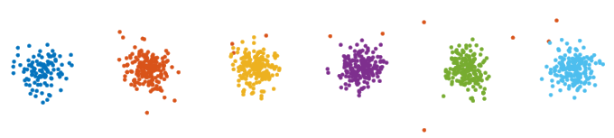
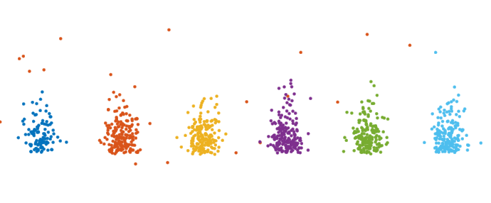
$\sigma=.6$	$\sigma=.1$
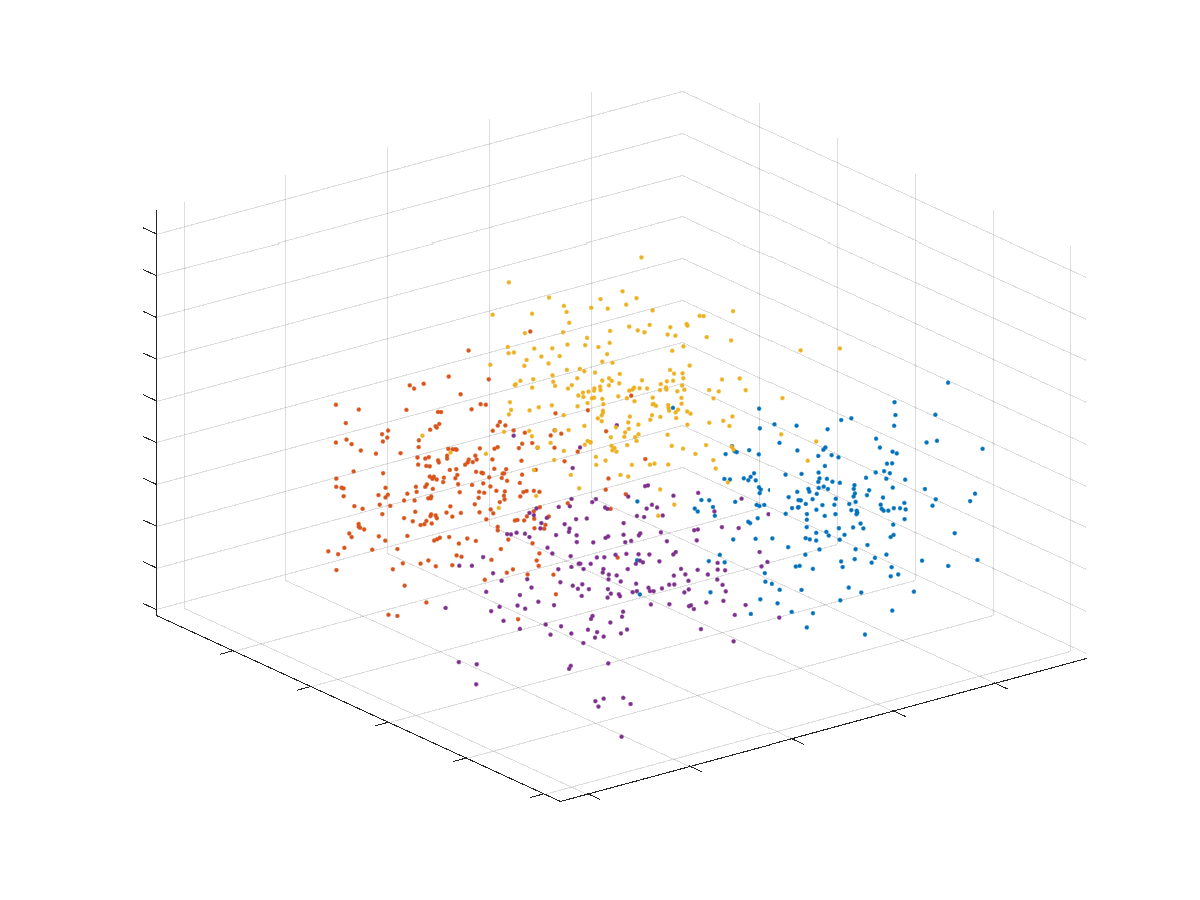
	$K=6$ clusters normal non-normal $\sigma$ $n=525$ $n=525$ 0.06 0.00(0.00) 0.005(0.001) 0.08 0.01(0.00) 0.006(0.001) 0.1 0.01(0.00) 0.009(0.003)
$\sigma=1.1$

Figure 2: Some data used in the experiments. In the first three plots, the clusters are sampled from mixtures of spherical Gaussians. In the last, one of the 15 coordinates is from a Gamma$(2,.4)$ distribution and rescaled by $\sigma$. Separation is the distance between the Gaussian means, and $\sigma$ is the standard deviation of the Gaussians. The $K=6$ data sets are designed to be hard for the spectral bounds but not for the SDP bounds. Bottom, left: optimality intervals $\varepsilon$ for data sampled from normal and non-normal mixtures with $K=6$ (mean and standard deviation over 10 replications). The values of $\varepsilon_{Sp}$ were much larger than $p_{\rm min}$ and are shown.

We implemented the $SS_{\rm Km}$ problem using the SDP solver SDPNAL+Zhao et al., (2010); Yang et al., (2015). We also implemented the spectral bound of Meilă, (2006), the only other method offering optimality intervals for K-means. The main questions of interest were (1) do our OI exist for realistic situations? (2) how tight are the bounds obtained?

Synthetic Data of Stochastic Ball Model

For this setting we sampled data uniformly from $K$ balls in dimension $d$ with unit radius. Let $\Delta$ be the minimal distance between the centers of the $K$ balls, then the SDP relaxation of K-Means we adopted in this paper can guarantee the exact recovery of $K$ clusters with high probability when $\Delta>2+\epsilon(d)$, where $\epsilon(d)\rightarrow 0$ as $d\rightarrow\infty$. This means that under this specific stochastic ball model, the k-means guarantee can only be obtained when the seperation between balls are large enough so that they don’t touch each other.

We sampled $n=500$ data from the stochastic ball model with $K=4,d=2$ and $\Delta$ ranging from 1.4 - 3.2. The centers of each ball are aligned on one line segment with equal space between. Then we perform K-means clustering with the initialization of correct labels, since we are only interested in understanding the behaviour of our method’s ability to obtain a guarantee for clustering result. Under this setting, the theoretical bound is trivial (larger than 4). Theoretically we can say nothing about how good the SDP relaxation is for the clustering. However as shown in figure 3 our method can provide some guarantees on a particular clustering result. In all settings, initializing with the true label, the distance between true label and the K-means solutions are close, with earth mover distance approximately $\sim 10^{-6}$. We see that in the model touching cases, our SS method provides insights on the distance between the K-means global optimal solution to the true label. On the other hand, all $\Delta\geq 2.2$ are within the regime where previous theoretical guarantee does not work. The results shows that K-means global optimizers approximately achieve the exact recovery of stochastic ball models.

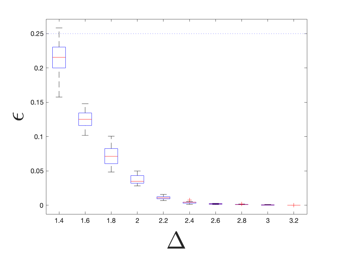
Figure 3: $\epsilon$ bound obtained for data sampled from stochastic ball model. The procedure is repeated for $10$ times under each setting. The $\epsilon$ bound are meaningful when they are smaller than $p_{\min}\approx 0.25$.

Synthetic Data of Gaussian Mixture

We sampled data from a mixture of $K=4$ normal distributions with equal spherical covariances $\sigma^{2}I_{d}$, in $d=15$ dimensions. The cluster sizes $n_{k}$ were approximately equal to $\lfloor n/K\rfloor$. The cluster means were at the corners of a regular tetrahedron with center separation $||\mu_{k}-\mu_{k^{\prime}}||=4\sqrt{2}\approx 5.67$. The data was clustered by K-means with random initialization, then the bounds $\varepsilon,\varepsilon_{Sp}$ corresponding respectively to the SS method and to the spectral method of Meilă, (2006) were computed.

$n=256$	$n=1024$

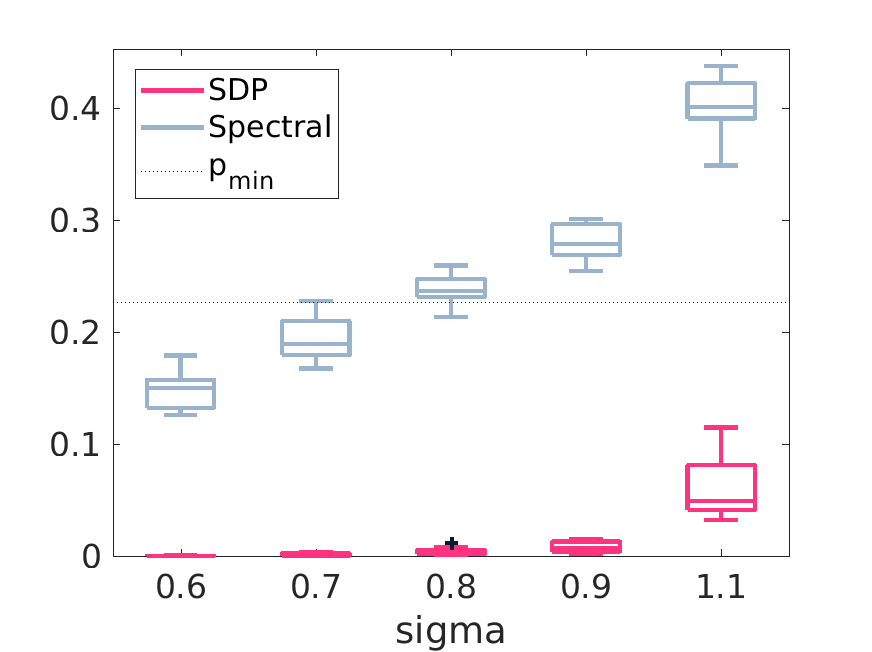
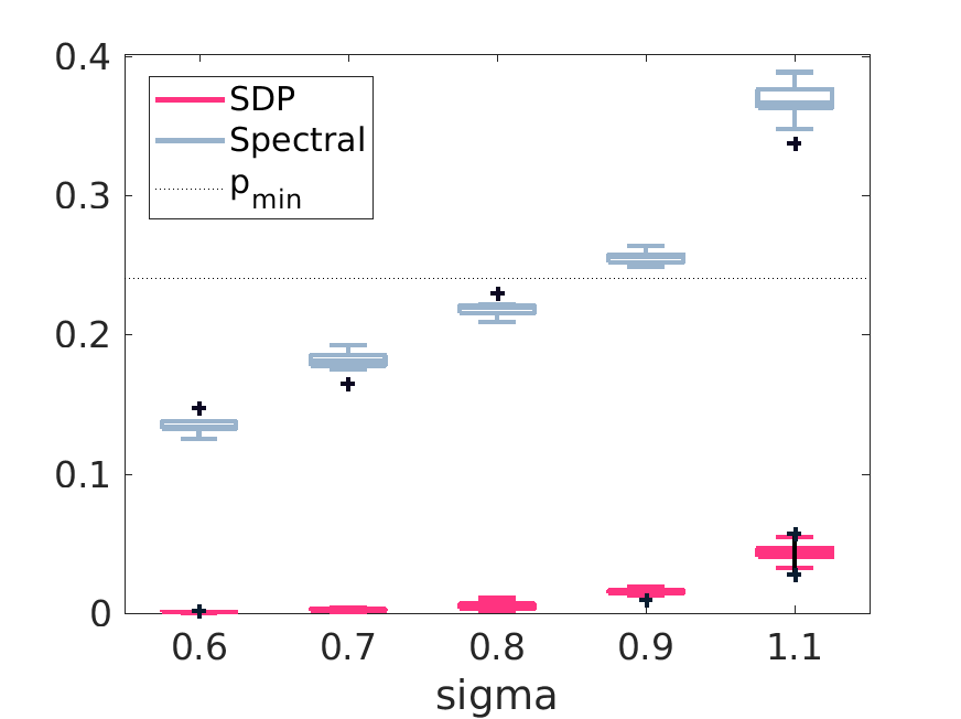
Figure 4: The optimality intervals $\varepsilon$ and $\varepsilon_{Sp}$ for data sampled from mixtures of normal distributions with $K=4$, $n=256$ and $1024$ and various $\sigma$ values (over 10 replications). The values of $\varepsilon_{Sp}$ exceeding $p_{\rm min}$ are not valid. Note that the $\varepsilon$ bounds are near 0 even though the clusters are not separated for $\sigma>0.8$.

In the experiments we also performed outlier removal, as follows. For each $x_{i}$, we computed the sum of the distances to its $p_{\rm min}/2$ nearest neigbors. We then removed the $n_{0}$ data points with the largest values for this sum. For good measure, we first added 20 outliers, then removed $n_{0}=4\%n$ respectively $n_{0}=2\%n$ points (so that $n_{0}$ is slightly larger than 20), before computing the bounds $\varepsilon,\varepsilon_{Sp}$. Consequently, these bounds do not refer to clusterings of the original ${\cal D}$, but to the “cleaned” dataset. Note that the outlier removal does not depend on the cluster labels; it is performed before clustering the data.

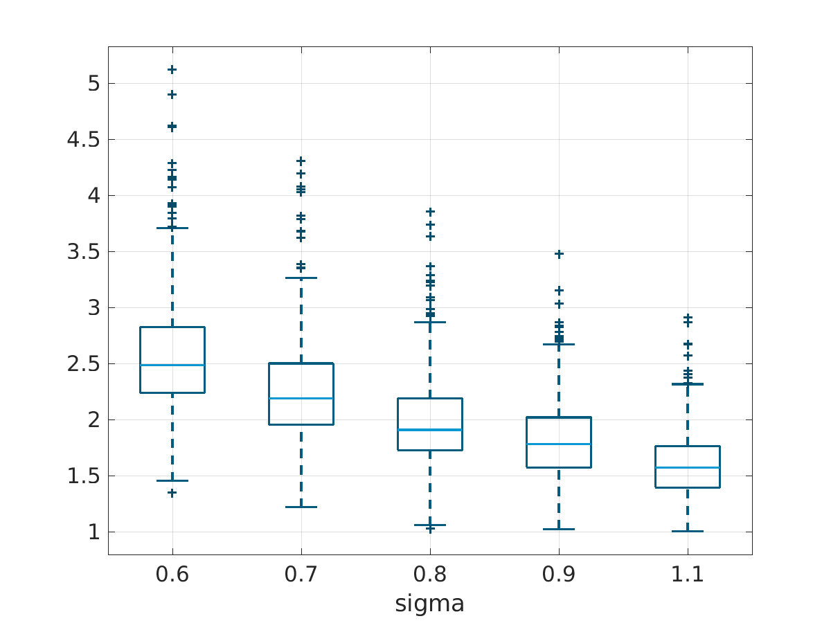
Figure 5: Separation statistics for the $K=4$ data, $n=1024$, all $\sigma$ values. Left: histogram of $\min_{k}||x_{i}-\mu_{k}||/\min_{k,k^{\prime}}||\mu_{k}-\mu_{k^{\prime}}||$ (i.e. distance of point to its center over minimum center separation) colored by $\sigma$. Note that when the clusters are contained in equal non-intersecting balls this ratio is strictly smaller than $0.5$. Right: boxplot of distance to second closest center over distance to own center, versus $\sigma$.

Figure 4 displays the bounds $\varepsilon,\varepsilon_{Sp}$ for these data, while Figure 2, top and bottom, left, displays some representative samples. The $\varepsilon$ optimality interval is much tighter than the spectral one $\varepsilon_{Sp}$, and, surprisingly enough, holds even when the clusters “touch”, i.e when there is no region of low density between the clusters. Figure 5 (left) shows that, when $\sigma>0.8$, the minimal spheres containing the clusters intersect; on the right we see that there are points which are almost equidistant from two cluster centers. Otherwise put, the distribution free bounds hold even when the data are not contained in non-intersecting balls, which is the best known condition for clusterability under model assumptions Awasthi et al., 2015a ; Awasthi et al., (2014).

Next, we performed experiments with unequal cluster sizes $p_{1:4}=0.1,0.2,0.3,0.4$, and we also generated non-gaussian clusters (details in the Appendix). We also performed experiments with $K=6$ clusters, with $p_{1:6}=0.1,0.18,0.18,0.18,0.18,0.18$. For $K=6$ we placed cluster centers along a line, as shown in Figure 2, top and bottom, right. This hurts the spectral bound which depends on a stable $K-1$-subspace, but does not hurt, and may even help the SDP bound $\varepsilon$.

The results are shown in Table 1, with run times for all experiments in the Appendix. The spectral bound $\varepsilon_{Sp}$ was much larger than $\varepsilon$ for all $K14$ experiments, and was never valid for $K=6$; therefore, it is omitted. The table also shows that $\varepsilon$ takes similar values in the case of equal and unequal clusters. However, in the latter case, the condition $\varepsilon\leq p_{\rm min}/p_{\rm max}$, is more stringent, hence some of the bounds obtained are not valid.

Over all experiments, we have found that the values of $\varepsilon$ are virtually insensitive to the sample size $n$, and degrade slowly when $p_{\rm min}$ decreases. The main limitation in these experiments is the requirement that $\varepsilon\leq p_{\rm min}$. This requirement can be traced back to Theorem 3. The bound in this Theorem, even though state of the art, is not tight, suggesting that some the $\varepsilon$ values marked in gray are valid OI even though we cannot prove it at this time.

Table 1: The OI $\varepsilon$ for $K=4$ clusters of unequal sizes (mean and standard deviation over 10 replications). The values in gray are not valid, owing to the fact that $\varepsilon p_{\rm max}>p_{\rm min}$ in these cases. Bounds for smaller $\sigma$ values were essentially zero and are ommitted.

	Unequal normal clusters			Unequal non-normal clusters
$\sigma$	$n=200$	$n=400$	$n=800$	$n=200$	$n=400$	$n=800$
0.6	0.00(0.00)	0.00(0.00)	0.00(0.00)	0.001(0.001)	0.001(0.000)	0.002(0.007)
0.8	0.01(0.01)	0.01(0.01)	0.01(0.01)	0.006(0.004)	0.004(0.002)	0.007(0.003)
1.0	0.09 (0.05)	0.06 (0.01)	0.07 (0.02)	0.04 (0.02)	0.03 (0.01)	0.03 (0.01)
1.2	0.28 (0.08)	0.21 (0.05)	0.21 (0.03)	0.16 (0.06)	0.14 (0.03)	0.13 (0.03)

Real data: configurations of the aspirin ($C_{9}H_{8}O_{4}$) molecule

These $n=2118$ samples (see Figure 6) were obtained via Molecular Dynamics (MD) simulation at $T=500$ degrees Kelvin by Chmiela et al., (2017) and represent 3D positions of the 21 atoms of aspirin. It was discovered recently that aspirin’s potential energy surface has two energy wells. The purpose of clustering of MD simulations is to label the data by energy well; this allows chemists to identify energy wells, on one hand, and on the other to identify states around on the transition path between the energy wells. These states describe the mechanism of a transition, and, being rare events in the contex of many simulations, are of great interest. Currently, the labeling is done by ad hoc algorithms. Having guarantees of (almost) correctness for the grouping, such as those in Figure 9 saves the time needed to validate the clustering by human inspection. Hence, we cluster these data into $K=2$ clusters, after having removed $n_{0}=0.5\%n=106$ outliers. The clusters found have relative sizes $p_{\rm min}=.26,p_{\rm max}=.74$, and the OI is $\varepsilon=.065$, an informative bound.

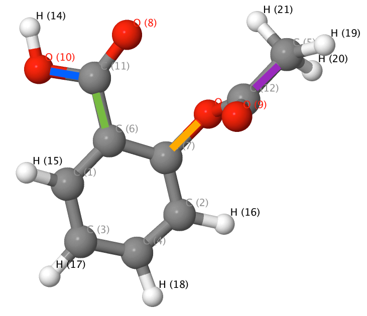
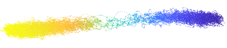
$K=2$ $p_{\rm min}=.26$ $p_{\rm max}=.74$

Figure 6: Left: the aspirin molecule. Middle: The first two principal components of the 57-dimensional aspirin data. The data is a Molecular Dynamics sequence of 211,762 configurations. We sample every 100-th point of the data for clustering. The axes are represented at scale.

6.2 Normalized Cut guarantees

Synthetic data

The matrix $S$ shown in Figure 8 was generated according to Meilă and Shi, 2001a . Even though $S$ is not block diagonal, it admits a perfect clustering, in the sense that the $K$ principal eigenvectors of $D^{-1}S$ are constant over each cluster. We perturbed $S$ with non-negative noise by $S_{ij}\leftarrow S_{ij}(1+\sigma u_{ij})$, $S_{ji}\leftarrow S_{ij}$, where $u_{ij}\sim uniform[0,1]$, i.i.d. for $i\leq j$ and $\sigma>0$. This perturbation keeps $S$ symmetric and with non-negative elements, but affects the eigenvectors and consequently the clustering, as shown in Figure 7.

We obtained a clustering of $S$ by spectral clustering with $K=5$, and repeated the process for different noise amplitudes $\sigma$ and random noise realizations. The results are displayed in Figure 8.

$S$ for $\sigma=32$	degrees $D_{ii}$,$\sigma=2$	(log) degrees $\sigma=2$
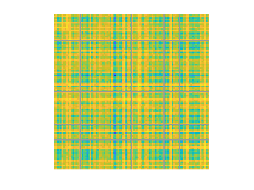
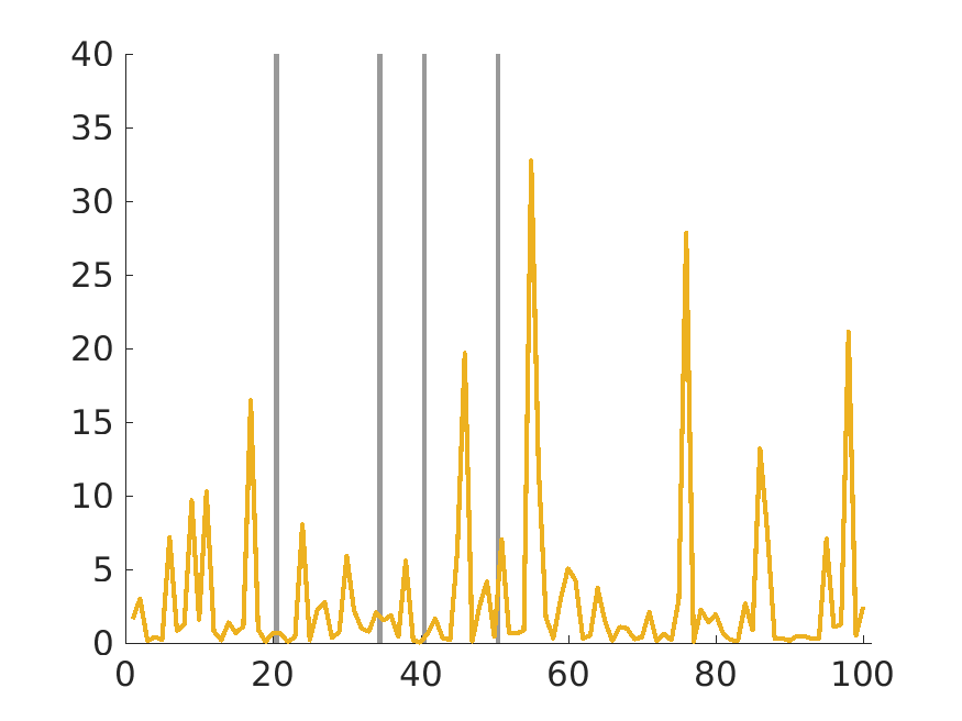
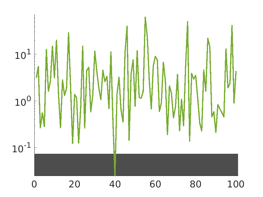
eigenvectors of $L$, $\sigma=32$	degrees $D_{ii}$, $\sigma=32$	(log) degrees $\sigma=32$

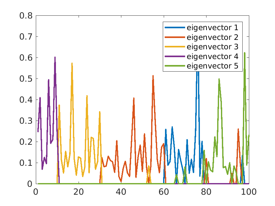
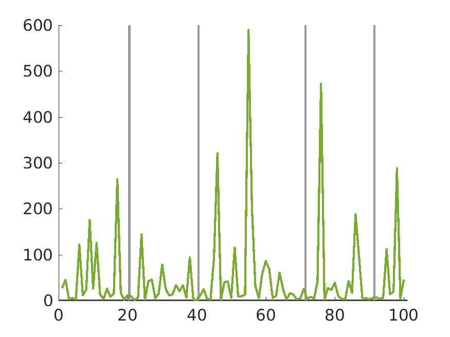
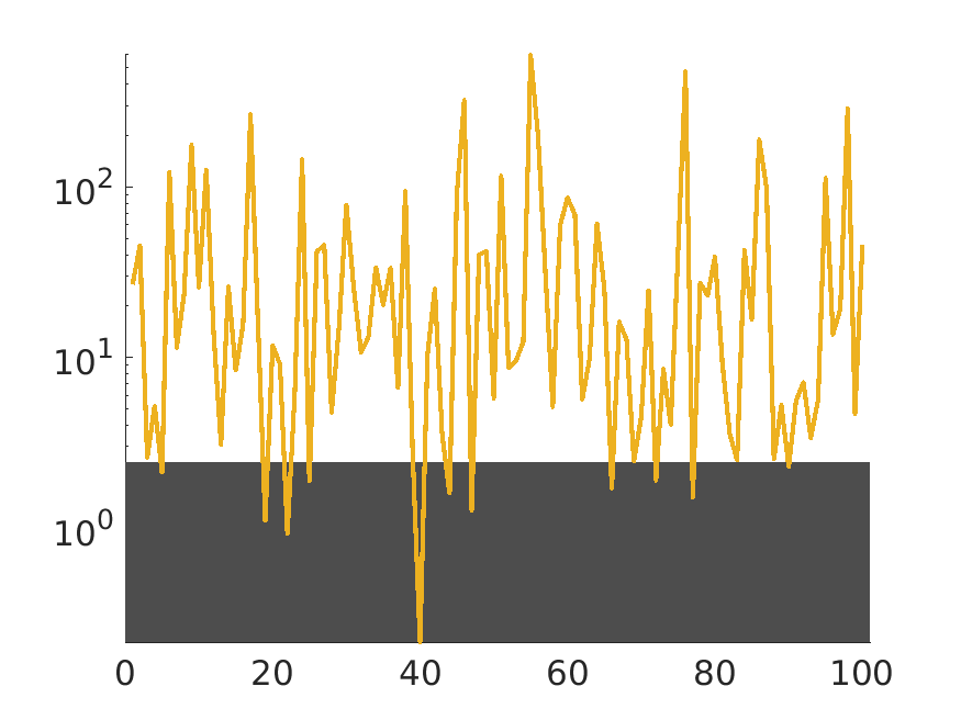
Figure 7: Illustrating the properties of the synthetic similarity matrices used in experiments; $K=5$, $n=100$, noise of amplitude $\sigma$. Example of similarity matrix $S$ (top, left) (values are on a logarithmic scale for better visualization); principal $K$ eigenvectors of the corresponding $L$ (bottom, left); values of node degrees $D_{ii}$ for $\sigma=2$ (top, middle) and $\sigma=32$ (bottom, middle) (note that the degrees are approximately proportional to $1+\sigma$); same node degrees on a logarithmic scale, with dark gray area representing the level of the SS bound $\varepsilon$ obtained for these data (top and bottom, right). Nodes with degrees above $\varepsilon$ are guaranteed not to change cluster membership in any clustering as good as the one found.

OI $\varepsilon$ and $\varepsilon_{Sp}$

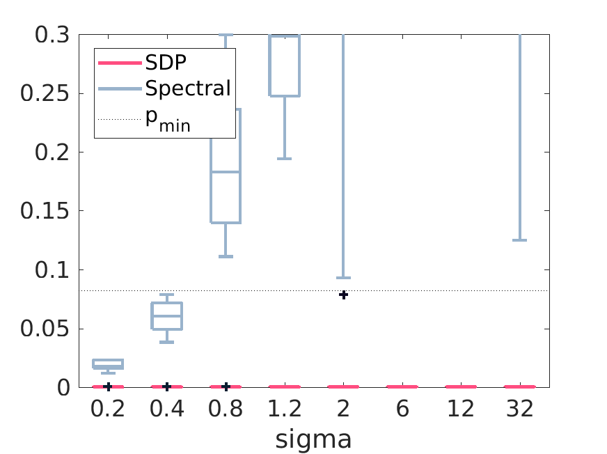
Figure 8: Experimental results for synthetic similarity matrix, clustered by Spectral Clustering; $K=5$, $n=100$, noise of amplitude $\sigma$; boxplots of OI $\varepsilon$ and spectral OI $\varepsilon_{Sp}$ versus noise amplitude $\sigma$ , over 10 replications for each noise level. Note that the OI from the SS method are practically 0.

Real data: MD simulation of a reversible reaction

In this section we consider molecular dynamics simulations (Fleming et al.,, 2016) of the reversible reaction $CH_{3}C\ell+C\ell^{-}\;\leftrightarrow\;CH_{3}C\ell+C\ell^{-},$ in which one of the chlorine ($C\ell$) atoms replaces the other in the methilchloride molecule. Molecular simulations of a reversible chemical reaction typically exhibit two clusters, one for each state of the system. Because of the symmetry of the reaction, the cluster sizes are approximately equal. The density between the two clusters, where the states on the reaction path lie, depends on the absolute temperature $T$ of the system. The intercluster density will be lower an the data more clusterable at lower temperatures. The data used in our experiments, available at https://www.stat.washington.edu/spectral/data/MDsimulations2017/, consist of 10 independently simulated trajectories at each of the four temperatures $T\in\{600,900,1050,1200\}$ degrees Kelvin. Trajectories were decimated to create data sets of $n\approx 1000$ points.

Figure 9, displays one of the similarity matrices at the highest temperature (with the data sorted by cluster label) and shows that the node degrees vary by about 2 orders of magnitude. The OI from Theorem 5 are represented in Figure 9 and summarized below.

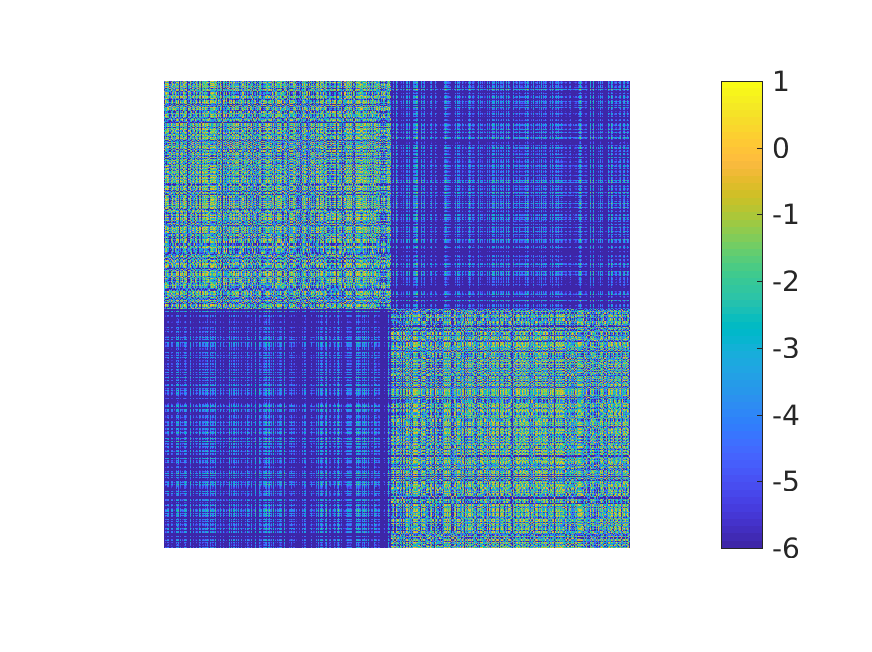
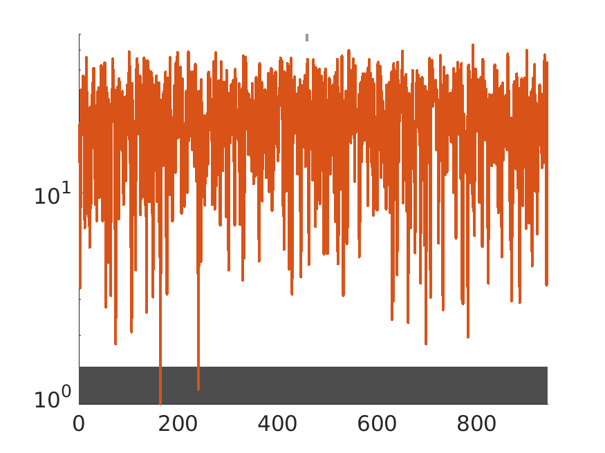
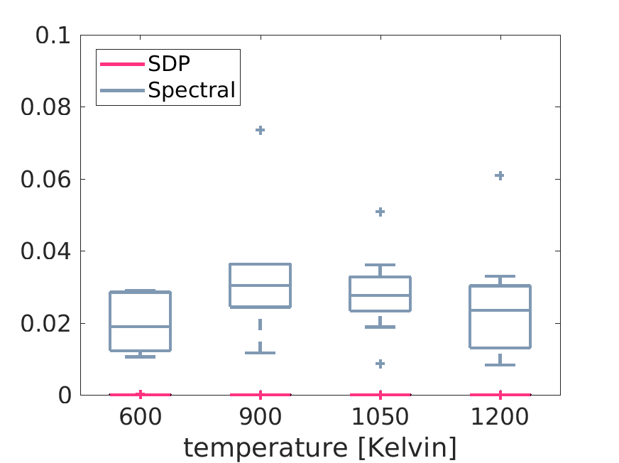
Figure 9: Results from the cholorometane experiments; $K=2$, $n\approx 950$, $p_{\rm min}\approx 0.47$. Example of similarity matrix $S$ from one simulation at 1200 Kelvin (on a logarithmic scale for better visualization) (left). Values of node degrees $D_{ii}$ for this $S$ matrix, with dark gray area representing the level of the OI $\varepsilon$ (middle). Nodes with degrees above $\varepsilon$ are guaranteed not to change cluster membership in any clustering as good as the one found. The bounds $\varepsilon$ and $\varepsilon_{Sp}$ versus temperature (right); there are 10 independent simulations for each temperature. Note that the optimality intervals from the SS method, $\varepsilon$, are indistinguishable from 0 in this plot. The values of $p_{\rm min}$ were all near $0.47$ and are not shown.

temperature [Kelvin]	600	900	1050	1200
median $\varepsilon$	7.3e-6	0	4e-9	6e-9
max $\varepsilon$	2e-4	2.8e-5	2e-7	2.2e-5

7 Discussion

Distribution free cluster validation in context

A researcher who wants to discover cluster structure in data must perform several inference tasks. This paper has focused on post-clustering validation, which happens to be the least studied of these inferences. When the data is clusterable, we have shown that validating the clusters is possible, without providing sharp thresholds. In Section 5 we have also cited works that prove that finding the clusters is tractable, under the assumption of clusterability. Hence, the loop is about to close, and we hope that in future work, to integrate the SS method with a clustering algorithm, providing thus a complete “clustering with guarantees” methodology. Furthermore, our distributional results show that for sufficiently large $n$, the SS method can be the basis of a test for clusterability, under generic Glivenko-Cantelli assumptions.

Proofs of instability

What happens when the Stability Theorem does not hold for a clustering ${\cal C}$? In this case, the researcher can try to certify that ${\cal C}$ is unstable. This task is comparatively easier, since a single counterexample ${\cal C}^{\prime}$ with $\operatorname{Loss}({\cal C}^{\prime})\approx\operatorname{Loss}({\cal C})$ and $d^{EM}({\cal C}^{\prime},{\cal C})>p_{\rm min}$ suffices. This, again, is a well studied area. The works of which propose random perturbations to the data and algorithm are a source of counterexamples. Note that these randomized methods may succeed in proving instability, but they cannot provably guarantee stability without strong additional assumptions on the data. As an alternative worth exploration, one could use the output of the SS method to find a witness of instability. More precisely, when the SS method fails to produce a valid OI, the matrix $X^{\prime}$ with $\operatorname{Loss}({\cal D},X^{\prime})\leq\operatorname{Loss}({\cal D},{\cal C})$ is far from $X({\cal C})$ in Frobenius norm. One could try to find a clustering ${\cal C}^{\prime}$ by e.g. rounding $X^{\prime}$, which would not differ much from $X^{\prime}$ in either $\operatorname{Loss}$ or distance to ${\cal C}$.

.

Stability and the choice of $K$

Throughout the paper, we have assumed that $K$ is fixed. We now remark that the SS method implicitly solves the problem of selecting $K$, and even that of selecting $\operatorname{Loss}$. Indeed, a clustering ${\cal C}$ that is found stable, with any $K$ and any loss function, is a “correct” clustering of the data under our paradigm. In the beginning, we presented the informed user as selecting the $\operatorname{Loss}$; with the concept of stability, one can take another view, of a user lucky enough to find a stable clustering while searching over loss functions and $K$ values. The SS method does not preclude the existence of more than one stable clustering for a data set ${\cal D}$. For example, if clusters are hiearchically nested, it is possible to find stable clusterings at several levels of the hierarchy.

In practice, $K$ is not known, and it is chosen after a set of clusterings ${\cal C}^{(K)}$, with $K=1,2,\ldots K_{max}$ have been obtained. With the SS method, one could dispense with the (more or less ad-hoc) methods for selecting $K$ in loss-based clustering. Indeed, by our initial argument, if ${\cal C}^{(K)}$ is proved to be stable for some $K$, this implicitly validates $K$ itself, as well as the loss function used. It is also possible to select more than one $K$, when the data supports meaningful partitions with different numbers of clusters.

Silhouette and other cluster quality indices

We contrast the framework proposed here with the existing literature on internal cluster validation; see e.g Maria Halkidi, (2015); Arbelaitz et al., (2013); Hennig and Liao, (2013) by indices such as the silhouette Rousseeuw, (1987). As it is well known, these indices are not associated with a clustering paradigm, whereas the present paper argues for paradigm specific validation, as a way to assure that the same criterion is used to find the clusters and to validate them. These indices could be potentially used as goodness measures, if their relations to specific clustering loss functions became better understood; the works cited above take steps in this direction.

Comparison with VC bounds

It is extremely rare in statistical inference to have worst case error bounds that are relevant in practice. For instance, the well known VC bounds for the 0-1 classification loss (see e.g. Vapnik, (1998)) typically take values above 1 (hence are completely uninformative from a practical standpoiht) and depend on the VC-dimension, a property of the hypotheses class that is usually intractable to compute.

In contrast, with the SS method, the OI $\varepsilon$ is always informative when it exists. With SDP relaxations, we obtain bounds that are not only informative, they are near 0 in non-trivial situations. To appreciate how far these guarantees can extend, recall than when $\sigma\approx\frac{1}{6}$ of the center separation, two spherical normal densities start to touch – no region of low density is left between them. Several of the informative, valid bounds in Section 6 are obtained near or even above these critical values. Moreover, an optimality interval is a distribution free, worst case bound. Thus, we believe that the computational demands of the SDP solver are justified by the guarantees offered.

Proofs

We first state several helpful propositions needed for our proofs.

Proposition 8

For any $X\in{\mathcal{X}}$, $||X||_{F}^{2}\leq K$.

Proposition 9

For any fixed two clusterings ${\cal C},{\cal C}^{\prime}$ it holds that

$$|d_{{\cal P}}^{EM}({\cal C},{\cal C}^{\prime})-d_{\widehat{{\cal P}}}^{EM}({\cal C},{\cal C}^{\prime})|\leq\sqrt{\frac{\log(4/\delta)}{2n}}$$ (24)

with probability $1-\delta/2$

Proof of Proposition 1

$X_{ij}\in[0,1]$ is obvious from the definition (1).

$$\operatorname{trace}X\,=\,\sum_{k=1}^{K}\sum_{i\in C_{k}}X_{ii}\,=\,\sum_{k=1}^{K}\sum_{i\in C_{k}}\frac{1}{n_{k}}\,=\,\sum_{k=1}^{K}n_{k}\frac{1}{n_{k}}\,=\,K.$$ (25)

Denote by $k_{0}$ the cluster containing data point $i$.

$$(X{\mathbf{1}})_{i}\,=\,\sum_{j=1}^{n}X_{ij}\,=\,\sum_{k=1}^{K}\sum_{i\in C_{k}}X_{ij}\sum_{j\in C_{k_{0}}}\frac{1}{n_{k}}\,=\,1.$$ (26)

Moreover, $X=ZZ^{T}$, hence $X\succeq 0$. $\Box$

Proof of Proposition 2

Let $X^{\prime},X^{\prime}_{2}$ be optima for the SS, respectively SS2 problem. Then, by the triangle inequality,

$$\varepsilon^{\prime}\;=\;||X^{\prime}-X({\cal C})|| \leq ||X^{*}-X({\cal C})||+||X^{*}-X^{\prime}||$$ (27)

$$\leq ||X^{*}-X^{\prime}_{2}||+||X^{*}-X^{\prime}_{2}||\;=\;2\varepsilon^{\prime}2.\hfill\Box$$ (28)

Proof of Theorem 4

Note that for any clustering ${\cal C}$, $||X({\cal C})||_{F}^{2}=\sum_{i,j=1}^{n}X_{ij}^{2}=,=\sum_{k=1}^{K}n_{k}^{2}\left(\frac{1}{n_{k}}\right)^{2}=K$. Moreover, from proposition 8 we have $||X||_{F}^{2}\leq K$.

Note also that $||X-X^{\prime}||^{2}_{F}=||X||^{2}_{F}+||X^{\prime}||^{2}_{F}-2\langle X,X^{\prime}\rangle=2K-2\langle X,X^{\prime}\rangle$. Hence, the optimization problem (SS_Km) finds the feasible $X^{\prime}$ which is furthest away from $X$. This completes Step 1. For Step 2 we can apply Theorem 9 of Meilă, (2012), which bounds the earthmover distance $d^{EM}$. $\Box$

Proof of Proposition 8

Denote by $\lambda_{1},\ldots\lambda_{n}$ the eigenvalues of $X$. Since $X$ has non-negative elements, and $X{\mathbf{1}}={\mathbf{1}}$, by the Frobenius Theorem, $|\lambda_{i}|\leq 1$, and because $X\succeq 0$, $\lambda_{i}\geq 0$ for all $i\in[n]$. Hence, $\lambda_{i}\in[0,1]$, for all $i$, and $||X||_{F}^{2}=\operatorname{trace}X^{2}=\sum_{i=1}^{n}\lambda_{i}^{2}\leq\sum_{i=1}\lambda_{i}=\operatorname{trace}X=K$. $\Box$

Proof of Theorem 5

The proof is similar to the proof of Proposition 4, after noting that for any ${\cal C}$, $||X({\cal C})||^{2}_{F}=K$. Again we use Theorem 9 of Meilă, (2012) which relates the error in Frobenius norm now to weigted EM distance. Note that $d^{EM}_{w}$ can always bound $d^{EM}$ by a factor of $\max_{i}w_{i}/\min_{i}w_{i}$.

Proof of Theorem 6

For any convex problem of the form (5), adding the constraint $\operatorname{Loss}\leq l$ and a linear objective preserves convexity. The functions $\langle X,X^{\prime}\rangle,\langle Z,Z^{\prime}\rangle,\langle\tilde{X},\tilde{X}^{\prime}\rangle$ are obviously linear in the second variable. Hence, the SS problem is always convex. Moreover, if (5) has a non-empty relative interior and $X\neq X^{*}$, the SS problem also has a non-empty relative interior, hence strong duality holds. Same arguments hold for $\tilde{X},Z$. Now, for $X$, is is easy to see from section 3.1 that the proof Proposition 4 holds regardless of the space ${\mathcal{X}}$ or of the expression of $\operatorname{Loss}$.

For $Z$, we first notice that $X=ZZ^{T}$ hence we can prove the result if we can lower bound $||Z^{T}Z^{\prime}||^{2}_{F}$ for any pair of clusterings. We have $\langle Z,Z^{\prime}\rangle=\operatorname{trace}Z^{T}Z^{\prime}$. Now, for any symmetric matrix $A$ with non-negative elements, $||A||^{2}_{F}=\operatorname{trace}A^{2}=\sum_{i\in[n]}\lambda_{i}(A)^{2}\geq\frac{1}{2}(\sum_{i\in[n]}\lambda_{i}(A))^{2}=\frac{1}{2}(\operatorname{trace}A)^{2}$. Let $\delta^{\prime}=\delta^{2}/2$. Then $\varepsilon=(K-\delta^{\prime})p_{\rm max}$ is an OI whenever it is smaller or equal to $p_{\rm min}$, by an argument similar to the proof of Proposition 4. Alternatively, we can notice that $||Z^{T}Z^{\prime}||_{F}^{2}=\operatorname{trace}(Z^{T}Z^{\prime})^{T}(Z^{T}Z^{\prime})=\operatorname{trace}(ZZ^{T})(Z^{\prime}(Z^{\prime})^{T})=\operatorname{trace}XX^{\prime}=\langle X,X^{\prime}\rangle$.

For the $\tilde{X}$ representation, we note that $||\tilde{X}||_{F}^{2}=\sum_{k\in[K]}n_{k}^{2}\leq(n-K+1)^{2}+(K-1)$ for any $\tilde{X}$ representing a clustering. Hence, $||\tilde{X}-\tilde{X}^{\prime}||^{2}_{F}=||\tilde{X}||^{2}_{F}+||\tilde{X}^{\prime}||^{2}_{F}-2\langle\tilde{X},\tilde{X}^{\prime}\rangle\leq||\tilde{X}||^{2}_{F}+(n-K+1)^{2}+(K-1)-2\delta$. We now apply Theorem 27 of Meilă, (2012) which states that $d^{EM}({\cal C},{\cal C}^{\prime})\leq\frac{1}{2n^{2}p_{\rm min}}||\tilde{X}({\cal C})-\tilde{X}({\cal C}^{\prime})||^{2}_{F}$ and obtain $\varepsilon=\frac{\sum_{k\in[K]}n_{k}^{2}+(n-K+1)^{2}+(K-1)-2\delta}{2p_{\rm min}}$ whenever $\varepsilon\leq p_{\rm min}$. $\Box$

Proof of Theorem 7

On the sample with probability $1-\delta/2$ it holds that

$$\sup_{{\cal C}\in\mathbf{C}_{K}({\cal D})}|L({\cal C})-\widehat{L}({\cal C})|\leq\Psi(n,\frac{\delta}{2}).$$ (29)

Now we condition on the event that (29) holds.

If there exists a population minimizer ${\cal C}^{opt}$ such that $d_{{\cal P}}^{EM}({\cal C}^{opt},\widehat{{\cal C}}^{opt})\leq\epsilon_{0}/2$. Note that by assumption of instability, there exists another clustering ${\cal C}^{*}$ such that $d_{{\cal P}}^{EM}({\cal C}^{*},{\cal C}^{opt})>\epsilon_{0}$ and $L({\cal C}^{*})<L({\cal C}^{opt})+\eta$, then $d_{{\cal P}}^{EM}({\cal C}^{*},\widehat{{\cal C}}^{opt})>\epsilon_{0}/2$. We can bound

$$\widehat{L}({\cal C}^{*})\leq L({\cal C}^{*})+\Psi(n,\frac{\delta}{2})\leq L({\cal C}^{opt})+\Psi(n,\frac{\delta}{2})+\eta\leq L(\widehat{C}^{opt})+\Psi(n,\frac{\delta}{2})+\eta\leq\widehat{L}(\widehat{{\cal C}})+2\Psi(n,\frac{\delta}{2})+\eta$$ (30)

and take $\widehat{{\cal C}}^{\prime}={\cal C}^{*}$.

If such a clustering ${\cal C}^{opt}$ does not exist, then note that for any optimal solution of the population clustering ${\cal C}^{opt}$,

$$\widehat{L}({\cal C}^{opt})\leq L({\cal C}^{opt})+\Psi(n,\frac{\delta}{2})\leq L(\widehat{{\cal C}})+\Psi(n,\frac{\delta}{2})\leq\widehat{L}(\widehat{{\cal C}})+2\Psi(n,\frac{\delta}{2})$$ (31)

and take $\widehat{{\cal C}}^{\prime}={\cal C}^{opt}$.

In both cases, applying proposition 9 it holds that $d_{{\cal P}}^{EM}(\widehat{{\cal C}}^{\prime},\widehat{{\cal C}}^{opt})\geq\epsilon_{0}/2-\sqrt{\log(4/\delta)/2n}$. Therefore $\widehat{{\cal C}}^{opt}$ is $(\Delta+2\Psi(n,\frac{\delta}{2}),\epsilon_{0}/2-\sqrt{\log(4/\delta)/2n})$ instable. $\Box$

Proof of Proposition 9

For fixed permutation $\pi$, from Hoeffding’s inequality

$$\left|\mathbb{E}_{{\cal P}}\sum_{i=1}^{K}\bm{1}_{X\in C_{i}\cap C_{\pi(i)}}-\mathbb{E}_{\widehat{{\cal P}}}\sum_{i=1}^{K}\bm{1}_{X\in C_{i}\cap C_{\pi(i)}}\right|\leq\sqrt{\frac{\log(2/\delta)}{2n}}$$ (32)

with probability $1-\delta$. Now let $\pi^{*},\widehat{\pi}^{*}$ be the permutation maximizing $\mathbb{E}_{{\cal P}}\sum_{i=1}^{K}\bm{1}_{X\in C_{i}\cap C_{\pi(i)}}$ and $\mathbb{E}_{\widehat{{\cal P}}}\sum_{i=1}^{K}\bm{1}_{X\in C_{i}\cap C_{\pi(i)}}$ respectively. Then

$$\mathbb{E}_{{\cal P}}\sum_{i=1}^{K}\bm{1}_{X\in C_{i}\cap C_{\pi^{*}(i)}}\leq\mathbb{E}_{\widehat{{\cal P}}}\sum_{i=1}^{K}\bm{1}_{X\in C_{i}\cap C_{\pi^{*}(i)}}+\sqrt{\frac{\log(2/\delta)}{2n}}\leq\mathbb{E}_{\widehat{{\cal P}}}\sum_{i=1}^{K}\bm{1}_{X\in C_{i}\cap C_{\widehat{\pi}^{*}(i)}}+\sqrt{\frac{\log(2/\delta)}{2n}}$$ (33)

$$\mathbb{E}_{\widehat{{\cal P}}}\sum_{i=1}^{K}\bm{1}_{X\in C_{i}\cap C_{\widehat{\pi}^{*}(i)}}\leq\mathbb{E}_{{\cal P}}\sum_{i=1}^{K}\bm{1}_{X\in C_{i}\cap C_{\widehat{\pi}^{*}(i)}}+\sqrt{\frac{\log(2/\delta)}{2n}}\leq\mathbb{E}_{{\cal P}}\sum_{i=1}^{K}\bm{1}_{X\in C_{i}\cap C_{\pi^{*}(i)}}+\sqrt{\frac{\log(2/\delta)}{2n}}$$ (34)

Therefore one concludes that $|d_{{\cal P}}^{EM}({\cal C},{\cal C}^{\prime})-d_{\widehat{{\cal P}}}^{EM}({\cal C},{\cal C}^{\prime})|\leq\sqrt{\log(2/\delta)/2n}$ with probability $1-\delta$. $\Box$

References

- Abbe et al., (2016) Abbe, E., Bandeira, A. S., and Hall, G. (2016). Exact recovery in the stochastic block model. IEEE Transactions on Information Theory, 62(1):471–487.
- Abbe and Sandon, (2016) Abbe, E. and Sandon, C. (2016). Achieving the ks threshold in the general stochastic block model with linearized acyclic belief propagation. In Lee, D. D., Sugiyama, M., Luxburg, U. V., Guyon, I., and Garnett, R., editors, Advances in Neural Information Processing Systems 29, pages 1334–1342. Curran Associates, Inc.
- Achlioptas and McSherry, (2005) Achlioptas, D. and McSherry, F. (2005). On spectral learning of mixtures of distributions. In Auer, P. and Meir, R., editors, 18th Annual Conference on Learning Theory, COLT 2005, pages 458–471, Berlin/Heidelberg. Springer.
- Ahmadian and Swamy, (2016) Ahmadian, S. and Swamy, C. (2016). Approximation algorithms for clustering problems with lower bounds and outliers. In 43rd International Colloquium on Automata, Languages, and Programming, ICALP 2016, July 11-15, 2016, Rome, Italy, pages 69:1–69:15.
- Arbelaitz et al., (2013) Arbelaitz, O., Gurrutxaga, I., Muguerza, J., PéRez, J. M., and Perona, I. n. (2013). An extensive comparative study of cluster validity indices. Pattern Recogn., 46(1):243–256.
- Awasthi et al., (2014) Awasthi, P., Balcan, M., and Voevodski, K. (2014). Local algorithms for interactive clustering. In Proceedings of the 31th International Conference on Machine Learning, ICML 2014, Beijing, China, 21-26 June 2014, pages 550–558.
- (7) Awasthi, P., Bandeira, A. S., Charikar, M., Krishnaswamy, R., Villar, S., and Ward, R. (2015a). Relax, no need to round: Integrality of clustering formulations. In Proceedings of the 2015 Conference on Innovations in Theoretical Computer Science, ITCS ’15, pages 191–200, New York, NY, USA. Association for Computing Machinery.
- (8) Awasthi, P., Charikar, M., Krishnaswamy, R., and Sinop, A. K. (2015b). The hardness of approximation of euclidean k-means. In 31st International Symposium on Computational Geometry, SoCG 2015, June 22-25, 2015, Eindhoven, The Netherlands, pages 754–767.
- Balakrishnan et al., (2017) Balakrishnan, S., Wainwright, M. J., and Yu, B. (2017). Statistical guarantees for the em algorithm: From population to sample-based analysis. Ann. Statist., 45(1):77–120.
- Ben-David et al., (2007) Ben-David, S., Pál, D., and Simon, H. U. (2007). Stability of k-means clustering. In Bshouty, N. H. and Gentile, C., editors, Learning Theory, pages 20–34, Berlin, Heidelberg. Springer Berlin Heidelberg.
- Ben-David and von Luxburg, (2008) Ben-David, S. and von Luxburg, U. (2008). Relating clustering stability to properties of cluster boundaries. In COLT 2008, pages 379–390, Madison, WI, USA. Max-Planck-Gesellschaft, Omnipress.
- Ben-David et al., (2006) Ben-David, S., von Luxburg, U., and Pal, D. (2006). A sober look at clustering stability. In 19th Annual Conference on Learning Theory, COLT 2006. Springer.
- Bubeck et al., (2012) Bubeck, S., Meilă, M., and von Luxburg, U. (2012). How the initialization affects the stability of the k-means algorithm. ESAIM: Probability and Statistics, 16:436–452.
- Charikar and Chatziafratis, (2017) Charikar, M. and Chatziafratis, V. (2017). Approximate hierarchical clustering via sparsest cut and spreading metrics. In Proceedings of the Twenty-Eighth Annual ACM-SIAM Symposium on Discrete Algorithms, SODA ’17, pages 841–854, USA. Society for Industrial and Applied Mathematics.
- Charikar and Guha, (1999) Charikar, M. and Guha, S. (1999). Improved combinatorial algorithms for the facility location and k-median problems. In 40th Annual Symposium on Foundations of Computer Science, pages 378–388.
- Chen and Xu, (2016) Chen, Y. and Xu, J. (2016). Statistical-computational tradeoffs in planted problems and submatrix localization with a growing number of clusters and submatrices. J. Mach. Learn. Res., 17(1):882–938.
- Chmiela et al., (2017) Chmiela, S., Tkatchenko, A., Sauceda, H. E., Poltavsky, I., Schütt, K. T., and Müller, K.-R. (2017). Machine learning of accurate energy-conserving molecular force fields. Science Advances, 3(5):e1603015.
- Dasgupta, (2000) Dasgupta, S. (2000). Experiments with random projection. In UAI ’00: Proceedings of the 16th Conference on Uncertainty in Artificial Intelligence, pages 143–151, San Francisco, CA, USA. Morgan Kaufmann Publishers Inc.
- Dasgupta, (2016) Dasgupta, S. (2016). A cost function for similarity-based hierarchical clustering. In Proceedings of the 48th Annual ACM SIGACT Symposium on Theory of Computing, STOC 2016, Cambridge, MA, USA, June 18-21, 2016, pages 118–127.
- Dasgupta and Schulman, (2007) Dasgupta, S. and Schulman, L. (2007). A probabilistic analysis of em for mixtures of separated, spherical gaussians. Journal of Machine Learnig Research, 8:203–226.
- Deshpande and Montanari, (2015) Deshpande, Y. and Montanari, A. (2015). Improved sum-of-squares lower bounds for hidden clique and hidden submatrix problems. In Grünwald, P., Hazan, E., and Kale, S., editors, Proceedings of The 28th Conference on Learning Theory, volume 40 of Proceedings of Machine Learning Research, pages 523–562, Paris, France. PMLR.
- Ding and He, (2004) Ding, C. and He, X. (2004). K-means clustering via principal component analysis. In Brodley, C. E., editor, Proceedings of the International Machine Learning Conference (ICML). Morgan Kauffman.
- E.Abbe and C.Sandon, (2015) E.Abbe and C.Sandon (2015). Community detection in general stochastic block models: fundamental limits and efficient recovery algorithms. In 2015 IEEE 56th Annual Symposium on Foundations of Computer Science, pages 670–688.
- Fleming et al., (2016) Fleming, K. L., Tiwary, P., and Pfaendtner, J. (2016). New approach for investigating reaction dynamics and rates with ab initio calculations. Jornal of Physical Chemistry A, 120(2):299–305.
- Garey and Johnson, (1979) Garey, M. R. and Johnson, D. S. (1979). Computers and Intractability: A Guide to the Theory of NP-Completeness. W. H. Freeman & Co., USA.
- Hazan and Ma, (2016) Hazan, E. and Ma, T. (2016). A non-generative framework and convex relaxations for unsupervised learning. In Proceedings of the 30th International Conference on Neural Information Processing Systems, NIPS’16, pages 3314–3322, Red Hook, NY, USA. Curran Associates Inc.
- Hein and Setzer, (2011) Hein, M. and Setzer, S. (2011). Beyond spectral clustering - tight relaxations of balanced graph cuts. In Shawe-Taylor, J., Zemel, R. S., Bartlett, P. L., Pereira, F., and Weinberger, K. Q., editors, Advances in Neural Information Processing Systems 24, pages 2366–2374. Curran Associates, Inc.
- Hennig and Liao, (2013) Hennig, C. and Liao, T. F. (2013). How to find an appropriate clustering for mixed type variables with application to socioeconomic stratification. Journal of the Royal Statistical Society, Series C (Applied Statistics), 62:309–369.
- Holland et al., (1983) Holland, P. W., Laskey, K. B., and Leinhardt, S. (1983). Stochastic blockmodels: First steps. Social networks, 5(2):109–137.
- Iguchi et al., (2015) Iguchi, T., Mixon, D. G., Peterson, J., and Villar, S. (2015). On the tightness of an SDP relaxation of k-means. ArXiv e-prints.
- Iguchi et al., (2017) Iguchi, T., Mixon, D. G., Peterson, J., and Villar, S. (2017). Probably certifiably correct k-means clustering. Math. Program., 165(2):605–642.
- Jalali et al., (2016) Jalali, A., Han, Q., Dumitriu, I., and Fazel, M. (2016). Relative density and exact recovery in heterogeneous stochastic block models. In Proc. of NIPS 2016.
- Kannan et al., (2000) Kannan, R., Vempala, S., and Vetta, A. (2000). On clusterings: good, bad and spectral. In Proc. of 41st Symposium on the Foundations of Computer Science, FOCS 2000.
- Karrer and Newman, (2011) Karrer, B. and Newman, M. (2011). Stochastic blockmodels and community structure in networks. Physical Review, 83:16107.
- Lee et al., (2014) Lee, J. R., Gharan, S. O., and Trevisan, L. (2014). Multi-way spectral partitioning and higher-order cheeger inequalities. Journal of the ACM.
- Maria Halkidi, (2015) Maria Halkidi, Michalis Vazirgiannis, C. H. (2015). Method-Independent Indices for Cluster Validation and Estimating the Number of Clusters, chapter 26. CRC Press.
- Maurer and Pontil, (2010) Maurer, A. and Pontil, M. (2010). K-dimensional coding schemes in hilbert spaces. IEEE Trans. Inf. Theor., 56(11):5839–5846.
- Meilă, (2006) Meilă, M. (2006). The uniqueness of a good optimum for K-means. In Moore, A. and Cohen, W., editors, Proceedings of the International Machine Learning Conference (ICML), pages 625–632. International Machine Learning Society.
- Meilă, (2012) Meilă, M. (2012). Local equivalence of distances between clusterings – a geometric perspective. Machine Learning, 86(3):369–389.
- (40) Meilă, M. and Shi, J. (2001a). Learning segmentation by random walks. In Leen, T. K., Dietterich, T. G., and Tresp, V., editors, Advances in Neural Information Processing Systems, volume 13, pages 873–879, Cambridge, MA. MIT Press.
- (41) Meilă, M. and Shi, J. (2001b). A random walks view of spectral segmentation. In Jaakkola, T. and Richardson, T., editors, Artificial Intelligence and Statistics AISTATS.
- Meilă et al., (2005) Meilă, M., Shortreed, S., and Xu, L. (2005). Regularized spectral learning. In Cowell, R. and Ghahramani, Z., editors, Proceedings of the Artificial Intelligence and Statistics Workshop(AISTATS 05).
- Peng and Wei, (2007) Peng, J. and Wei, Y. (2007). Approximating k-means-type clustering via semidefinite programming. SIAM journal on optimization.
- Peng et al., (2015) Peng, R., Sun, H., and Zanetti, L. (2015). Partitioning well-clustered graphs: Spectral clustering works! In Grünwald, P. and Hazan, E., editors, Proceedings of The 28th Conference on Learning Theory (COLT), volume 40, pages 1–33.
- Pollard, (1981) Pollard, D. (1981). Strong consistency of -means clustering. Ann. Statist., 9(1):135–140.
- Qin and Rohe, (2013) Qin, T. and Rohe, K. (2013). Regularized spectral clustering under the degree-corrected stochastic blockmodel. In Advances in Neural Information Processing Systems.
- Rakhlin and Caponnetto, (2006) Rakhlin, A. and Caponnetto, A. (2006). Stability of k-means clustering. In Proceedings of the 19th International Conference on Neural Information Processing Systems, NIPS’06, pages 1121–1128, Cambridge, MA, USA. MIT Press.
- Rangapuram et al., (2014) Rangapuram, S. S., Mudrakarta, P. K., and Hein, M. (2014). Tight continuous relaxation of the balanced k-cut problem. In Ghahramani, Z., Welling, M., Cortes, C., Lawrence, N. D., and Weinberger, K. Q., editors, Advances in Neural Information Processing Systems 27, pages 3131–3139. Curran Associates, Inc.
- Rousseeuw, (1987) Rousseeuw, P. J. (1987). Silhouettes: A graphical aid to the interpretation and validation of cluster analysis. Journal of Computational and Applied Mathematics, 20:53 – 65.
- Roy and Pokutta, (2016) Roy, A. and Pokutta, S. (2016). Hierarchical clustering via spreading metrics. In Guyon, I. and von Luxburg, U., editors, Advances in Neural Information Processing Systems (NIPS).
- Shamir and Tishby, (2009) Shamir, O. and Tishby, N. (2009). On the reliability of clustering stability in the large sample regime. In Koller, D., Schuurmans, D., Bengio, Y., and Bottou, L., editors, Advances in Neural Information Processing Systems 21, pages 1465–1472. Curran Associates, Inc.
- Shamir and Tishby, (2010) Shamir, O. and Tishby, N. (2010). Stability and model selection in k-means clustering. Machine Learning, 80(2):213–243.
- Shi and Malik, (2000) Shi, J. and Malik, J. (2000). Normalized cuts and image segmentation. IEEE Trans. on Pattern Analysis and Machine Intelligence.
- Swamy, (2004) Swamy, C. (2004). Correlation clustering: maximizing agreements via semidefinite programming. In Proceedings of the Fifteenth Annual ACM-SIAM Symposium on Discrete Algorithms, SODA, pages 526–527.
- Telgarsky and Dasgupta, (2013) Telgarsky, M. J. and Dasgupta, S. (2013). Moment-based uniform deviation bounds for k-means and friends. In Burges, C. J. C., Bottou, L., Welling, M., Ghahramani, Z., and Weinberger, K. Q., editors, Advances in Neural Information Processing Systems 26, pages 2940–2948. Curran Associates, Inc.
- Vapnik, (1998) Vapnik, V. (1998). Statistical Learning Theory. Wiley.
- Vempala and Wang, (2004) Vempala, S. and Wang, G. (2004). A spectral algorithm for learning mixtures of distributions. Journal of Computer Systems Science, 68(4):841–860.
- Vinayak et al., (2014) Vinayak, R. K., Oymak, S., and Hassibi, B. (2014). Graph clustering with missing data: Convex algorithms and analysis. In Advances in Neural Information Processing Systems (NIPS), pages 2996–3004.
- von Luxburg et al., (2008) von Luxburg, U., Belkin, M., and Bousquet, O. (2008). Consistency of spectral clustering. Ann. Statist., 36(2):555–586.
- Wan and Meila, (2015) Wan, Y. and Meila, M. (2015). A class of network models recoverable by spectral clustering. In Lee, D. and Sugiyama, M., editors, Advances in Neural Information Processing Systems (NIPS).
- Xing and Jordan, (2003) Xing, E. P. and Jordan, M. I. (2003). On semidefinite relaxation for normalized k-cut and connections to spectral clustering. Technical Report UCB/CSD-03-1265, EECS Department, University of California, Berkeley.
- Yang et al., (2015) Yang, L., Sun, D., and Toh, K. (2015). Sdpnal+: a majorized semismooth newton-cg augmented lagrangian method for semidefinite programming with nonnegative constraints. Mathematical Programming Computation, 7:331–366.
- Zhao et al., (2010) Zhao, X., Sun, D., and Toh, K.-C. (2010). A newton-cg augmented lagrangian method for semidefinite programming. SIAM J. Optimization, 20:1737–1765.
- Zhu et al., (2014) Zhu, C., Xu, H., Leng, C., and Yan, S. (2014). Convex optimization procedure for clustering: Theoretical revisit. In Advances in Neural Information Processing Systems 27, pages 1619–1627.