Exact optimal stopping for multidimensional linear switching diffusions

Abstract

The paper studies a class of multidimensional optimal stopping problems with infinite horizon for linear switching diffusions. There are two main novelties in the optimal problems considered: the underlying stochastic process has discontinuous paths and the cost function is not necessarily integrable on the entire time horizon, where the latter is often a key assumption in classical optimal stopping theory for diffusions, cf. [23, Corollary 2.9]. Under relatively mild conditions, we show, for the class of multidimensional optimal stopping problems under consideration, that the first entry time of the stopping region is an optimal stopping time. Further, we prove that the corresponding optimal stopping boundaries can be represented as the unique solution to a nonlinear integral equation. We conclude with an application of our results to the problem of quickest real-time detection of a Markovian drift.

Keywords. Quickest detection, switching diffusions, optimal stopping, free-boundary problem.

MSC 2010 Codes: Primary: 60G40, 93C30. Secondary: 60H30, 91B70.

1 Introduction

Given a complete probability space $(\Omega,{\cal F},\mathsf{P})$, we consider a system of linear stochastic differential equations with dynamics given by

(1.1) $$dX_{t}^{i}=\Big{(}a^{i}(\alpha_{t})+\sum_{j=1}^{2}b^{ij}(\alpha_{t})X_{t}^{j}\Big{)}dt+\sigma^{i}(\alpha_{t})X_{t}^{i}dW_{t}^{i}\text{ for }i=1,2,$$

where $\alpha$ is a two-state Markov chain with state space $M:=\{1,2\}$) and $W=(W^{1},W^{2})$ is a two-dimensional standard Brownian motion. The coefficients $a^{i}(\cdot),b^{ij}(\cdot),\sigma^{i}(\cdot):\{1,2\}\mapsto(-\infty,\infty)$ are appropriate mappings such that the solution process $X$ is non-negative (see Assumption 2.1 in Section 2). It is well known that equation (1.1) admits a unique solution $X$ and that the couple $(\alpha,X)$ is a strong Markov process (see, for example, [25]).

The solution process $X$ of (1.1) coupled with the Markov chain $\alpha$ is generally referred to as a regime switching diffusion The primary motivation for the introduction of the Markov chain $\alpha$ is to model the effect of uncertain discrete events on the underlying stochastic system (for example, the transition from a bull market to a bear market during a financial crisis). For more general properties and applications of regime switching diffusions, we refer the reader to [25].

The key optimal stopping problem we shall consider in the present paper is

(1.2) $$V(\iota,x)=\inf_{\tau}\mathsf{E}\>\!_{\iota,x}\int_{0}^{\tau}e^{-\int_{0}^{t}\lambda(\alpha_{s})ds}H(\alpha_{t},X_{t})dt,$$

where the infimum is taken over all stopping times ${\cal T}_{\alpha,X}$ of $(\alpha,X)$ for some appropriate discounting factor function $\lambda(\cdot):\mathbb{N}\mapsto(0,\infty)$ and for a running cost function $H:\mathbb{N}\times[0,\infty)^{2}\mapsto(-\infty,\infty)$. The key mathematical difficulties in solving this optimal stopping problem are that the paths of $(\alpha,X)$ are not continuous and that the cost functional (appearing on the right-hand side of equation (1.2)) may not be integrable on time horizon $[0,\infty)$. For general background on the theory of optimal stopping for diffusions, we refer the reader to [23] and to the references therein.

In the one-dimensional optimal stopping literature (see, for example, [16, 20, 26, 27]), one usually identifies the value function and the stopping region explicitly by finding a closed form solution to a one-dimensional free-boundary ordinary differential equation (ODE). For multidimensional optimal stopping problems, it is nearly impossible to find a closed form solution for the free-boundary partial differential equation (PDE) in most cases. In these cases, one may resort to excessive functions, Green kernel representations, and/or solutions to Hamilton-Jacobi-Bellman (HJB) equations (see [4, 6, 7, 8, 18, 19]). A key drawback of these characterizations of the value function is that they do not provide an exact optimal stopping policy. In models with switching, the continuation region and the stopping region are divided into several layers according to the state of the Markov chain and finding the explicit solution to an optimal stopping problem is not generally straightforward, even when working with one-dimensional free-boundary ODEs. This is because the continuation regions differ by layers, leading to the so-called ‘transition region’ (i.e. the set of points belonging to the continuation region in one layer and belonging to the stopping region in another layer).

Unlike the aforementioned works, this paper considers a multidimensional optimal stopping problem for a diffusion under a random switching environment. As previously mentioned, the key mathematical difficulties in finding the optimal stopping policy are: (i) the paths of $(\alpha,X)$ are not continuous and (ii) the cost functional (appearing in the right-hand side in (1.2)) may not be integrable on time horizon $[0,\infty)$. It is the second difficulty which shall disable our use of a key tool in classical optimal stopping theory ([23, Corollary 2.9]), which requires uniform integrability on the entire time horizon (cf. [23, (2.2.1)]). Despite these challenges, we succeed in giving a nonlinear integral equation for the optimal stopping boundary and prove that the value function is the solution of a free-boundary PDE. This allows us to represent the optimal stopping boundary as a unique solution to a nonlinear integral equation. One key difficulty we shall encounter is that Peskir’s change-of-variable formula of local time on surfaces in [21] cannot be employed due to the presence of the Markov chain. This necessitates our development of a generalized Itô’s formula for the value function acting on the switching diffusion even though the function is not second-order continuously differentiable.

The remainder of this work is organized as follows. In Section 2, we introduce necessary preliminaries regarding the paper’s key optimal stopping problem of interest given in equation (1.2). Section 3 discusses the optimal stopping boundary and its properties. Section 4 presents the corresponding free-boundary PDE. Section 5 provides the nonlinear integral equation needed to identify the optimal stopping boundary. Section 6 concludes the paper by applying the paper’s results to a problem of quickest real-time detection of a Markovian drift. An analogous quickest real-time detection problem for a Brownian coordinate drift but without the incorporation of switching environments was solved in [14] for the one-dimensional case and in [12] for the multidimensional case.

2 Preliminaries

This section introduces necessary preliminaries. Recall that ${\cal T}_{\alpha,X}$ is the collection of all possible stopping times of $(\alpha,X)$ with respect to the natural filtration augmented with all $\mathsf{P}$-null sets (${\cal F}=\{{\cal F}_{t}:t\geq 0\}$). Since $(\alpha,X)$ is a Lévy process, ${\cal F}$ is right-continuous and the first entry time of a closed set is a stopping time if it is finite almost surely (cf. [2, p.72]). We recall the key optimal stopping problem under consideration disclosed in Section 1.

Optimal stopping problem (OSP): We wish to find a stopping time $\tau_{*}\in{\cal T}_{\alpha,X}$ such that

(2.1) $$V(\iota,x)=\mathsf{E}\>\!_{\iota,x}\int_{0}^{\tau_{*}}e^{-\int_{0}^{t}\lambda(\alpha_{s})ds}H(\alpha_{t},X_{t})dt=\inf_{\tau\in{\cal T}_{\alpha,X}}\mathsf{E}\>\!_{\iota,x}\int_{0}^{\tau}e^{-\int_{0}^{t}\lambda(\alpha_{s})ds}H(\alpha_{t},X_{t})dt,$$

subject to

(2.2) $$dX_{t}^{i}=\Big{(}a^{i}(\alpha_{t})+\sum_{j=1}^{2}b^{ij}(\alpha_{t})X_{t}^{j}\Big{)}dt+\sigma^{i}(\alpha_{t})X_{t}^{i}dW_{t}^{i}\text{ for }i=1,2.$$

We assume that the generator of the continuous-time Markov Chain is $Q=(q_{\iota\jmath})_{2\times 2}$, i.e. for $\iota\neq\jmath$, $\sum_{\jmath\in M}q_{\iota\jmath}=0$ and $q_{\iota\jmath}\geq 0$ ([25, Section 1.4]). Further, we shall assume that Assumption 2.1 below holds throughout the sequel.

Assumption 2.1.

For each $\iota\in M$, and for $i=1,2,$ we have that $\lambda(\iota)>0$, $a^{i}(\iota)\geq 0$ and $\sigma^{i}(\iota)\neq 0$. Further, for each $\iota\in M$ and for $i\neq j$, $b^{ij}(\iota)\geq 0$.

Standard results for stochastic differential equations imply that under Assumption 2.1, equation (2.2) admits a unique solution $X=(X^{1},X^{2})$ in $[0,\infty)^{2}$ for any non-negative initial state. Note that the regime switching diffusion $(\alpha,X)$ is a homogeneous strong Markov process. Let $X(\iota,x)=(X^{1}(\iota,x),X^{2}(\iota,x))$ denote the solution of (2.2) with initial values $(\alpha_{0},X_{0})=(\iota,x)$. For all initial values $(\iota,x)\in M\times(0,\infty)^{2}$, the solution process $X$ stays positive with probability 1, i.e. for $t>0$,

$$\mathsf{P}_{\iota,x}\big{(}X_{t}\in(0,\infty)^{2}\big{)}=1.$$

For each $\iota\in M$, the following comparison principle ([13]) holds:

(2.3) $$\text{ If }x_{1}\leq y_{1}\text{ and }x_{2}\leq y_{2},\,\,X_{t}^{i}(\iota,x)\leq X^{i}_{t}(\iota,y).$$

Further, the infinitesimal generator $I\!\!L$ of $(\alpha,X)$ is non-degenerate on $(0,\infty)^{2}$ and has the following form for any $f(\iota,\cdot)\in\mathscr{C}^{2}\big{(}(0,\infty)^{2}\big{)}$ (cf. (2.4) in [25])

(2.4) $$I\!\!Lf(\iota,x)=\sum_{i=1}^{2}\Big{(}a^{i}(\iota)+\sum_{j=1}^{2}b^{ij}(\iota)x_{j}\Big{)}\partial_{i}f(\iota,x)+\frac{1}{2}\sum_{i=1}^{2}(\sigma^{i}(\iota)x_{i})^{2}\partial_{ii}f(\iota,x)+\sum_{\jmath\in M}q_{\iota\jmath}f(\jmath,x).$$

Therefore, $(\alpha,X)$ is strong Feller and admits a transition density $p_{t}(\iota,x;\jmath,y)$ on $M\times(0,\infty)^{2}$ as follows

$$\mathsf{P}_{\imath,x}(\alpha_{t}=\jmath,X_{t}\in dy)=p_{t}(\iota,x;\jmath,y)dy.$$

In the sequel, we shall also assume that Assumption 2.2 below holds.

Assumption 2.2.

For each $\iota\in M$, $H(\iota,\cdot)$ is concave on $[0,\infty)^{2}$, locally Lipschitz up to the boundary of $[0,\infty)^{2}$, and is increasing with respect to each variable. Moreover

$$\lim_{z\rightarrow\infty}H(\iota,(z,0))=\lim_{z\rightarrow\infty}H(\iota,(0,z))=\infty.$$

Under Assumption 2.2, $H$ is bounded from below and therefore the value function in (2.1) is well-defined. Note that (2.1) is Lagrangian formulated ([14]).
We now pause to introduce some necessary notation for future use

$$\underline{H}:=\inf_{\iota\in M}H(\iota,(0,0)),\quad\underline{\lambda}:=\inf_{\iota\in M}\lambda(\iota),\quad\text{and}\quad\underline{a}^{i}:=\inf_{\iota\in M}a^{i}(\iota).$$

Without loss of generality, we may assume that $\underline{H}<0$. Otherwise, $\tau=0$ is always optimal for the optimal stopping problem in (2.1) and the problem is trivial. Under Assumption 2.2, the inequality

(2.5) $$\mathsf{E}\>\!_{\iota,x}\int_{0}^{\infty}e^{-\int_{0}^{t}\lambda(\alpha_{s})ds}H(\alpha_{t},X_{t})dt<\infty,$$

does not necessarily hold. It is important to note that the inequality in (2.5) is analogous to Assumption [23, (2.2.1)], which is needed for [23, Corollary 2.9] to hold.
In the sequel, we shall denote by $\tau_{D}$ the first entry time to the set $D$ for the stochastic process $(\alpha,X)$, i.e.

(2.6) $$\tau_{D}:=\inf\{t\geq 0:(\alpha(t),X(t))\in D\},$$

where by definition $\inf\emptyset=\infty$. We shall further assume throughout that Assumption 2.3 below holds.

Assumption 2.3.

For $i=1,2$, the solution of $\widetilde{X}_{t}^{i}$ to

$$d\widetilde{X}_{t}^{i}=(a^{i}(\alpha_{t})+b^{ii}(\alpha_{t})\widetilde{X}_{t}^{i})dt+\sigma^{i}(\alpha_{t})\widetilde{X}_{t}^{i}dW_{t}^{i}$$

is recurrent to $(c,\infty)$ for any $c>0$.

Proposition 2.5, which we shall present at the conclusion of this section, shall show that Assumption 2.3 may be easily verified.

2.1 One-dimensional optimal stopping problems

We now introduce a one-dimensional optimal stopping problem which shall prove useful for later study. For any positive real number $N$, we consider the one-dimensional optimal stopping problem

(2.7) $$\begin{array}[]{ll}\displaystyle\widetilde{V}^{1,N}(\iota,z)&\!\!\!\displaystyle=\inf_{\tau}\mathsf{E}\>\!_{\iota,z}\int_{0}^{\tau}e^{-\int_{0}^{t}\lambda(\alpha_{s})ds}H^{N}(\alpha_{t},(\widetilde{X}^{1}_{t},0))dt,\end{array}$$

where

(2.8) $$H^{N}(\iota,x)=\min(H(\iota,x),N)$$

and where $\widetilde{X}^{1}$ solves the stochastic differential equation

$$d\widetilde{X}_{t}^{1}=(a^{1}(\alpha_{t})+b^{11}(\alpha_{t})\widetilde{X}_{t}^{1})dt+\sigma^{1}(\alpha_{t})\widetilde{X}_{t}^{1}dW_{t}^{1}.$$

By the comparison principle in (2.3), we have, for all $t\geq 0$, that if $\widetilde{X}_{0}^{1}=X_{0}^{1}$ then $\widetilde{X}_{t}^{1}\leq X_{t}^{1}$. The optimal stopping problem in (2.7) is thus a special case of the optimal stopping problem in (2.1) when the second coordinate process is fixed at zero. We now consider the optimal stopping region for $\widetilde{V}^{1,N}$ in Proposition 2.4 below.

Proposition 2.4.

Suppose Assumptions 2.1, 2.2 and 2.3 hold, and let $N>0$ be large. Then the following two statements hold:

(1) The optimal stopping region for $\widetilde{V}^{1,N}$ is $\{(\iota,z)\in M\times(0,\infty):\widetilde{V}^{1,N}(\iota,z)=0\}$.

(2) For the one-dimensional optimal stopping problem in (2.7), the optimal stopping region for $\widetilde{V}^{1,N}$ has the form

$$\{(\iota,z)\in M\times(0,\infty):z\geq\bar{x}_{\iota}^{1}\},$$

where for $\iota\in M$, $\bar{x}_{\iota}^{1}$ are finite positive real numbers. Further, the first entry time of the stopping region is finite almost surely.

Proof.

(1) $H^{N}$ is bounded and $(\alpha,X)$ is a Feller process. This follows immediately from [6].

(2) Note $\widetilde{X}^{1}_{t}(\iota,x_{1})$ is affine in $x_{1}$ and that $H^{N}(\iota,\cdot,0)$ is concave increasing. Further, $\widetilde{V}^{N}(\iota,\cdot)$ is also concave increasing on $(0,\infty)$. This suggests that for the optimal stopping boundaries $\{\bar{x}_{\iota}^{1}\}_{\iota\in M}$ that the stopping region for (2.7) should be $\{(\iota,z)\in M\times(0,\infty):z\geq\bar{x}_{\iota}^{1}\}.$ We also note that $\bar{x}_{\iota}^{1}$ is dependent on $N$ and, for each $\iota\in M$, $\bar{x}_{\iota}^{1}$ is decreasing as $N$ increases. That is, if $z>\bar{x}_{\iota}^{1}$, $\widetilde{V}^{1,N}(\iota,z)=0$; otherwise $\widetilde{V}^{1,N}(\iota,z)<0$. We now wish to show, for $N>0$ (large) with $N>N_{0}$, that $\bar{x}_{\iota}^{1}<\infty$ for each $\iota\in M$. We prove this by contradiction.

First, recall that for each $\iota\in M$, $\widetilde{V}^{1,N}(\iota,\cdot)$ is increasing, concave and continuous on $[0,\infty)$. For the sake of contradiction, let us suppose that $\bar{x}_{1}^{1}=\infty$. This means that

(2.9) $$\widetilde{V}^{1,N}(1,z)<0\text{ for all }z\in[0,\infty).$$

Let $\tau_{*}$ denote the first entry time of the stopping region and let $\tau_{1}:=\inf\{t\geq 0:\alpha_{t}\neq 1\}$ be the first transition time of the Markov chain (which is independent of $N$ and $z$). We thus have that $\tau_{1}\leq\tau_{*}$ and

$$\begin{array}[]{ll}\widetilde{V}^{1,N}(1,z)&\!\!\!\displaystyle\geq\mathsf{E}\>\!_{1,z}\int_{0}^{\tau_{1}}e^{-\int_{0}^{t}\lambda(\alpha_{s})ds}\Big{(}H^{N}(\alpha_{t},(\widetilde{X}^{1}_{t},0))-\underline{H}\Big{)}dt+\underline{H}/\underline{\lambda}.\end{array}$$

Note that the right-hand side is increasing in $N$ and $z$. By Assumption 2.2, the right-hand side tends to $\infty$ when both $N\rightarrow\infty$ and $z\rightarrow\infty$. Therefore we may take large $N_{0}$ and $z_{0}$ such that $\widetilde{V}^{N_{0}}(1,z_{0})>0$. Then for large $N$ with $N>N_{0}$, it follows that $\widetilde{V}^{N}(1,z)>0$ for $z>z_{0}$, contradicting (2.9). Thus, by contradiction, we conclude that $\bar{x}_{1}^{1}<\infty$. One may similarly prove that, for each $\iota\in M$, $\bar{x}_{\iota}^{1}<\infty$. By Assumption 2.3, $(\alpha,\widetilde{X}^{1})$ will enter the stopping region in finite time. This completes the proof.  

Of course, the above results for the one-dimensional optimal stopping problem in (2.7) can be employed when working with the one-dimensional optimal stopping problem

(2.10) $$\begin{array}[]{ll}\displaystyle\widetilde{V}^{2,N}(\iota,z)&\!\!\!\displaystyle=\inf_{\tau}\mathsf{E}\>\!_{\iota,z}\int_{0}^{\tau}e^{-\int_{0}^{t}\lambda(\alpha_{s})ds}H^{N}(\alpha_{t},(0,\widetilde{X}^{2}_{t}))dt,\end{array}$$

where $\widetilde{X}^{2}$ solves

$$d\widetilde{X}_{t}^{2}=(a^{2}(\alpha_{t})+b^{22}(\alpha_{t})\widetilde{X}_{t}^{2})dt+\sigma^{2}(\alpha_{t})\widetilde{X}_{t}^{2}dW_{t}^{2}.$$

The one-dimensional optimal stopping problems in (2.7) and in (2.10) shall prove helpful in our later study of multidimensional optimal stopping problems. We conclude the present section by showing, as promised earlier, that Assumption 2.3 may be easily verified.

Proposition 2.5.

The following two statements hold.
(1) Assumption 2.3 holds for $i=1,2$ if for any $c>0$, there exists a twice continuously differentiable function $W_{c}:M\times(0,c]\mapsto(-\infty,\infty)$ such that $\lim_{z\rightarrow 0^{+}}W_{c}(\iota,z)=\infty$ and

$$(a^{i}(\iota)+b^{ii}(\iota)z)W_{c}^{\prime}(\iota,z)+\frac{1}{2}(\sigma^{i}(\iota)z)^{2}W_{c}^{\prime\prime}(\iota,z)+\sum_{\jmath\in M}q_{\iota\jmath}W_{c}(\jmath,z)\leq 0$$

for $(\iota,z)\in M\times(0,c).$

(2) Assumption 2.3 holds if

(2.11) $$a^{i}(\cdot)>0\text{ and }b^{ii}(\cdot)\geq 0.$$

Proof.

(1) The proof is identical to that of [25, Theorem 3.14].

(2) Consider $\tau_{c}:=\inf\{t\geq 0:\widetilde{X}^{1}_{t}\geq c\}$. Since $\widetilde{X}^{1}_{t}$ never returns to $0$, Itô’s formula yields that

$$\begin{array}[]{ll}\displaystyle c\geq\mathsf{E}\>\!_{\iota,x_{1}}\widetilde{X}^{1}_{\tau_{c}\wedge N}-x_{1}\geq\mathsf{E}\>\!_{\iota,x_{1}}\int_{0}^{\tau_{c}\wedge N}a^{1}(\alpha_{s})dt\geq\underline{a}^{1}\mathsf{E}\>\!_{\iota,x_{1}}(\tau_{c}\wedge N).\end{array}$$

We thus have that $\mathsf{E}\>\!_{\iota,x_{1}}(\tau_{c}\wedge N)\leq c/\underline{a}^{1}$. Letting $N\rightarrow\infty$, we obtain

$$\mathsf{P}_{\iota,x_{1}}(\tau_{c}\geq N)\leq\frac{c}{N\underline{a}^{1}}\rightarrow 0.$$

Thus $\mathsf{P}_{\iota,x_{1}}(\tau_{c}<\infty)=1$ and Assumption 2.3 holds.  

3 Optimal stopping boundary of the optimal stopping problem in (2.1)

In this section, we will derive some helpful properties of the optimal stopping boundary for the optimal stopping problem in (2.1). Throughout the sequel, we shall again assume that Assumptions 2.1, 2.2, and 2.3 hold.

The candidate continuation region $C$ and stopping region $D$ for the optimal stopping problem in (2.1) are, respectively,

(3.1) $$\begin{array}[]{ll}C&\!\!\!\displaystyle=\Big{\{}(\iota,x)\in M\times(0,\infty)^{2}\!:V(\iota,x)<0\Big{\}},\end{array}$$

and

(3.2) $$\begin{array}[]{ll}D&\!\!\!\displaystyle=\Big{\{}(\iota,x)\in M\times(0,\infty)^{2}\!:V(\iota,x)=0\Big{\}}.\end{array}$$

$C$ and $D$ are divided into different layers by the discrete states of the Markov chain. Let $C_{\iota}$ and $D_{\iota}$ be the $\iota$th layer of $C$ and $D$, respectively. $C_{\iota}$ and $D_{\iota}$ are subsets of $(0,\infty)^{2}$, i.e.

(3.3) $$\begin{array}[]{ll}C_{\iota}=\Big{\{}x\in(0,\infty)^{2}\!:V(\iota,x)<0\Big{\}}\text{ and }D_{\iota}=\Big{\{}x\in(0,\infty)^{2}\!:V(\iota,x)=0\Big{\}}.\end{array}$$

Given the formulation of $D$ in (3.2) above, a natural question to ask is as follows: is $\tau_{D}$, the first entry time of the stopping region $D$, the optimal stopping time for the optimal stopping problem in (2.1)? We shall soon see that the answer will be ‘yes’, but the solution will be far from trivial because Corollary 2.9 from [23] cannot be invoked since the inequality in (2.5) does not hold. To overcome this difficulty, a key idea we shall employ is to cut off the function $H$ from above by a positive constant $N$ and then to let $N\rightarrow\infty$. We shall refer to this idea as an ‘approximation’ stopping problem.

3.1 Approximation method

To overcome the difficulties mentioned above, we turn to the so-called ‘approximation’ optimal stopping problem in (3.4) below.

Optimal Stopping Problem (OSP)-$N$: We wish to find a stopping time $\tau_{*}\in{\cal T}_{\alpha,X}$ such that

(3.4) $$V^{N}(\iota,x)=\mathsf{E}\>\!_{\iota,x}\int_{0}^{\tau_{*}}e^{-\int_{0}^{t}\lambda(\alpha_{s})ds}H^{N}(\alpha_{t},X_{t})dt=\inf_{\tau\in{\cal T}_{\alpha,X}}\mathsf{E}\>\!_{\iota,x}\int_{0}^{\tau}e^{-\int_{0}^{t}\lambda(\alpha_{s})ds}H^{N}(\alpha_{t},X_{t})dt,$$

where $H^{N}(\iota,x)$ has been defined in (2.8) above. Since $H^{N}$ is bounded and $(\alpha,X)$ is a Feller process, Proposition 3.1 below immediately follows from [19].

Proposition 3.1.

$V^{N}$ is continuous and is the unique viscosity solution to the following HJB equation

(3.5) $$\min(I\!\!Lw-\lambda w+H^{N},-w)=0,$$

where $w:M\times(0,\infty)^{2}\mapsto\mathbb{R}$.

We now let $N\rightarrow\infty$ for the optimal stopping problem in (3.4). Let $\Lambda_{t}:=\int_{0}^{t}\lambda(\alpha_{s})ds$ and

$$\left\{\begin{array}[]{ll}&\!\!\!\displaystyle C^{N}:=\Big{\{}(\iota,x):V^{N}(\iota,x)<0\Big{\}},~{}C_{\varepsilon}^{N}:=\Big{\{}(\iota,x):V^{N}(\iota,x)<-\varepsilon\Big{\}},\\ \vskip 3.0pt plus 1.0pt minus 1.0pt\cr&\!\!\!\displaystyle D^{N}:=\Big{\{}(\iota,x):V^{N}(\iota,x)\geq 0\Big{\}},~{}D_{\varepsilon}^{N}:=\Big{\{}(\iota,x):V^{N}(\iota,x)\geq-\varepsilon\Big{\}}.\end{array}\right.$$

Since $V^{N}$ is continuous, $C^{N}$ and $C_{\varepsilon}^{N}$ are open sets and $D^{N}$ and $D_{\varepsilon}^{N}$ are closed sets. Moreover, $D_{\varepsilon}^{N}$ is increasing as $N$ increases and is decreasing as $\varepsilon$ decreases. We now proceed with some necessary results on the finiteness of the first entry time into the stopping region $D^{N}$.

Lemma 3.2.

The first entry time $\tau_{D^{N}}$ of $D^{N}$ is finite almost surely. Therefore $\tau_{D}$ and $\tau_{D_{\varepsilon}^{N}}$ are finite almost surely.

Proof.

By the monotonicity of $H$, we have $V\geq V^{N}\geq\widetilde{V}^{1,N}$, where $\widetilde{V}^{1,N}$ has been defined in (2.7). This means that

$$D\supset D^{N}\supset\{(\iota,x_{1},x_{2})\in M\times(0,\infty)^{2}:x_{1}\geq\bar{x}_{\iota}^{1}\}.$$

By Proposition 2.4, $\tau_{D^{N}}$ is finite almost surely. Noting that $\tau_{D_{\varepsilon}^{N}},\tau_{D}\leq\tau_{D^{N}}$, the proof is now complete.  

3.2 The optimal stopping region for the optimal stopping problem in (2.1)

The purpose of this section is to present the optimal stopping region for the optimal stopping problem in (2.1) by letting $N\rightarrow\infty$ for the optimal stopping problem in (3.4). We begin with Lemma 3.3 below, which assures that the first entry time is optimal for the optimal stopping problem in (2.1).

Lemma 3.3.

If there exists a $N_{0}>0$ such that $\tau_{D^{N_{0}}}$ is finite almost surely with

(3.6) $$\mathsf{E}\>\!_{\iota,x}\int_{0}^{\tau_{D^{N_{0}}}}e^{-\Lambda_{t}}|H(\alpha_{t},X_{t})|dt<\infty\text{ for any }(\iota,x)\in M\times(0,\infty)^{2},$$

then $\tau_{D}$ is the optimal stopping time of the optimal stopping problem in (2.1), provided that $\partial D$ is Green’s regular.

Proof.

Immediately, we see that $D^{N}\subset D^{N}_{\varepsilon}$. Thus, with probability 1, $\tau_{D^{N}_{\varepsilon}}\leq\tau_{D^{N}}$. Let $\tau_{j}$ denote the first exit time of $(\alpha,X)$ from the set $M\times(1/j,j)^{2}$. Further, note that $C_{\varepsilon}^{N}$ is an open subset of $C^{N}$ and that the closure of $C_{\varepsilon}^{N}$ is a subset of $C^{N}$. Employing Snell’s envelope (cf. [23, Theorem 2.4]), we see that the following process is a martingale

$$e^{-\Lambda_{t\wedge\tau_{j}\wedge\tau_{D^{N}_{\varepsilon}}}}V^{N}(\alpha_{t\wedge\tau_{j}\wedge\tau_{D^{N}_{\varepsilon}}},X_{t\wedge\tau_{j}\wedge\tau_{D^{N}_{\varepsilon}}})+\int_{0}^{t\wedge\tau_{j}\wedge\tau_{D^{N}_{\varepsilon}}}e^{-\Lambda_{s}}H^{N}(\alpha_{s},X_{s})ds.$$

We proceed to calculate

(3.7) $$\begin{array}[]{ll}&\!\!\!\displaystyle V^{N}(\iota,x)=\mathsf{E}\>\!_{\iota,x}\Big{[}\int_{0}^{t\wedge\tau_{j}\wedge\tau_{D^{N,}_{\varepsilon}}}e^{-\Lambda_{s}}H^{N}(\alpha_{s},X_{s})ds+e^{-\Lambda_{t\wedge\tau_{j}\wedge\tau_{D^{N}_{\varepsilon}}}}V^{N}(\alpha_{t\wedge\tau_{j}\wedge\tau_{D^{N,}_{\varepsilon}}},X_{t\wedge\tau_{j}\wedge\tau_{D^{N}_{\varepsilon}}})\Big{]}\\ \vskip 3.0pt plus 1.0pt minus 1.0pt\cr&\!\!\!\displaystyle=\mathsf{E}\>\!_{\iota,x}\Big{[}\int_{0}^{\tau_{j}\wedge\tau_{D^{N}_{\varepsilon}}}e^{-\Lambda_{s}}H^{N}(\alpha_{s},X_{s})ds+e^{-\Lambda_{\tau_{j}\wedge\tau_{D^{N}_{\varepsilon}}}}V^{N}(\alpha_{\tau_{j}\wedge\tau_{D^{N}_{\varepsilon}}},X_{\tau_{j}\wedge\tau_{D^{N}_{\varepsilon}}})\Big{]}\\ \vskip 3.0pt plus 1.0pt minus 1.0pt\cr&\!\!\!\displaystyle=\mathsf{E}\>\!_{\iota,x}\Big{[}\int_{0}^{\tau_{D^{N}_{\varepsilon}}}e^{-\Lambda_{s}}H^{N}(\alpha_{s},X_{s})ds+e^{-\Lambda_{\tau_{D^{N}_{\varepsilon}}}}V^{N}(\alpha_{\tau_{D^{N}_{\varepsilon}}},X_{\tau_{D^{N}_{\varepsilon}}})\Big{]}\\ \vskip 3.0pt plus 1.0pt minus 1.0pt\cr&\!\!\!\displaystyle\geq\mathsf{E}\>\!_{\iota,x}\Big{[}\int_{0}^{\tau_{D^{N}_{\varepsilon}}}e^{-\Lambda_{s}}H^{N}(\alpha_{s},X_{s})ds\Big{]}-\varepsilon,\end{array}$$

where in the second line of the above display we have let $t\rightarrow\infty$ and have invoked the fact that $V^{N}$ is continuous and bounded. Further, in the third line of the above display, we have (i) let $j\rightarrow\infty$ and recalled that for $N>N_{0}$, $\tau_{D_{\varepsilon}^{N}}\leq\tau_{D^{N}}$ is finite almost surely (Proposition 3.2) (ii) applied monotone convergence and (iii) employed the fact that $D^{N}_{\varepsilon}$ is closed.

Provided (3.6) holds, it follows by (3.7) that

(3.8) $$\begin{array}[]{ll}V(\iota,x)&\!\!\!\displaystyle\geq V^{N}(\iota,x)\geq\mathsf{E}\>\!_{\iota,x}\Big{[}\int_{0}^{\tau_{D_{\varepsilon}^{N}}}e^{-\Lambda_{t}}H^{N}(\alpha_{t},X_{t})dt\Big{]}-\varepsilon\\ \vskip 3.0pt plus 1.0pt minus 1.0pt\cr&\!\!\!\displaystyle\geq V(\iota,x)-\varepsilon-\mathsf{E}\>\!_{\iota,x}\int_{0}^{\tau_{D_{\varepsilon}^{N}}}e^{-\Lambda_{t}}|H^{N}(\alpha_{t},X_{t})-H(\alpha_{t},X_{t})|dt.\end{array}$$

Sequentially letting $N\rightarrow\infty$ and $\varepsilon\rightarrow 0^{+}$, dominated convergence yields that

(3.9) $$V(\iota,x)=\lim_{N\rightarrow\infty}V^{N}(\iota,x)=\lim_{\varepsilon\rightarrow 0^{+}}\lim_{N\rightarrow\infty}\mathsf{E}\>\!_{\iota,x}\int_{0}^{\tau_{D^{N}_{\varepsilon}}}e^{-\Lambda_{t}}H(\alpha_{t},X_{t})dt.$$

Further, it is useful to note that

$$\begin{array}[]{ll}\displaystyle\bigcup_{N}D_{\varepsilon}^{N}=\bigcup_{N}\{V^{N}\geq-\varepsilon\}\subset\{V\geq-\varepsilon\}=D_{\varepsilon},\end{array}$$

and

$$\begin{array}[]{ll}\displaystyle\bigcup_{N}D_{\varepsilon}^{N}=\bigcup_{N}\{V^{N}\geq-\varepsilon\}\supset\{V\geq 0\}=D.\end{array}$$

Recall that $(\alpha,X)$ has right-continuous paths with left-limits ([25, Proposition 2.4]). By Theorem 4 in [5, Section 2.4], we have that

$$V(\iota,x)=\mathsf{E}\>\!_{\iota,x}\int_{0}^{\tau_{D}}e^{-\Lambda_{t}}H(\alpha_{t},X_{t})dt$$

i.e. $\tau_{D}$ is the optimal stopping time. This concludes the proof.  

Lemma 3.3 may be considered an extension of [23, Corollary 2.9] in the setting where (i) the cost functional is not necessarily integrable on the entire time horizon and (ii) the underlying stochastic process does not have continuous paths. This extension enables us to work with a larger class of multidimensional optimal stopping problems. Before continuing to discuss properties of the stopping and continuation regions in Section 3.3, we pause to offer some remarks below.

Remark 3.4.

(1) Since $H$ is bounded from below, (3.6) is equivalent to

$$\mathsf{E}\>\!_{\iota,x}\int_{0}^{\tau_{D^{N_{0}}}}e^{-\Lambda_{t}}H(\alpha_{t},X_{t})dt<\infty$$

for any $(\iota,x)\in M\times(0,\infty)^{2}$. Further, we have that $D^{N}\subset D\subset D_{\varepsilon}$. This means that we do not require uniform integrability on the interval $(0,\infty)$. Rather, we only require uniform integrability on a (random) subinterval $(0,\tau_{D^{N_{0}}})$.

(2) If $\lambda(\cdot)>0$ and $H$ is bounded on $C^{N_{0}}$, then (3.6) holds. We will see this in the next section.

3.3 Properties of the stopping and continuation regions

This section considers properties of the stopping regions $D$ and continuation regions $C$. The key result of this section is Theorem 3.8. We first turn to a few preparatory lemmas and propositions required for the proof of this theorem.

Lemma 3.5.

For each $\iota\in M$, $V(\iota,x)$ is increasing in $x$. Moreover $V(\iota,\cdot)$ is concave and continuous on $(0,\infty)^{2}$. The same results also hold for $V^{N}$.

Proof.

Let us fix a value of $\iota\in M$. Invoking the comparison principle in (2.3), we see that $V(\iota,x)$ is increasing in $x$ since $H(\iota,x)$ is also increasing in $x$. Note that $X^{\iota,x}_{t}$ is affine with respect to $x$ and that, for each $\iota\in M$, $V(\iota,\cdot)$ is concave. Consequently $V(\iota,\cdot)$ is continuous on $(0,\infty)^{2}$. The aforementioned results also hold for $V^{N}$ because $H^{N}$ is concave. This completes the proof.  

We now proceed to define

$$b_{\iota}(x_{1}):=\inf\Big{\{}x_{2}>0:V(\iota,x_{1},x_{2})=0\Big{\}}.$$

The curve $S_{b_{\iota}}$ gives the optimal stopping boundary on the $\iota$th layer. One may similarly define $b_{\iota}^{N}$ as the optimal stopping boundary for $S^{N}$. We now prove in Lemma 3.6 below that the optimal stopping time $\tau_{D}$ given in (2.6) is finite.

Lemma 3.6.

For each $\iota\in M$, when $N>N_{0}$, and for any $z>0$, we have that $b_{\iota}(z)<b^{N}_{\iota}(z)<\infty$. Moreover,

$$\mathsf{P}_{\iota,x}(\tau_{D}<\infty)=1$$

for all $(\iota,x)\in M\times(0,\infty)^{2}$.

Proof.

Since $b_{\iota}$ is decreasing, it suffices to prove that $b^{N}_{\iota}(0^{+})<\infty$. By Proposition 2.4, for $N>N_{0}$, we have that $\widetilde{V}^{1,N}(\iota,z,0)=0$ for $z>\bar{x}_{\iota}^{1}$. Therefore, for $z>\bar{x}_{\iota}^{1}$,

$$\begin{array}[]{ll}&\!\!\!\displaystyle V^{N}(\iota,z,0)=\inf_{\tau}\mathsf{E}\>\!_{\iota,z,0}\int_{0}^{\tau}e^{-\int_{0}^{t}\lambda(\alpha_{s})ds}H^{N}(\alpha_{t},(X^{1}_{t},X^{2}_{t}))dt\\ \vskip 3.0pt plus 1.0pt minus 1.0pt\cr&\!\!\!\displaystyle\geq\inf_{\tau}\mathsf{E}\>\!_{\iota,z}\int_{0}^{\tau}e^{-\int_{0}^{t}\lambda(\alpha_{s})ds}H^{N}(\alpha_{t},(\widetilde{X}^{1}_{t},0))dt=\widetilde{V}^{1,N}(\iota,z)=0.\end{array}$$

Thus

$$b^{N}_{\iota}(z)\leq b^{N}_{\iota}(0^{+})\leq\bar{x}_{\iota}^{1}.$$

Let us now define the two stopping times

$$\tau_{*}:=\inf\{t\geq 0:X^{1}_{t}\geq\sup_{\iota\in M}\bar{x}_{\iota}^{1}\}\text{ and }\tilde{\tau}_{*}:=\inf\{t\geq 0:\widetilde{X}^{1}_{t}\geq\sup_{\iota\in M}\bar{x}_{\iota}^{1}\}.$$

Clearly, if $X^{1}_{0}=\widetilde{X}_{0}^{1}$, the following inequality for the first entry time

$$\tau_{D^{N}}\leq\tau_{*}\leq\tilde{\tau}^{*},$$

holds with probability 1. By Assumption 2.3, $\tilde{\tau}^{*}<\infty$ with probability 1, completing the proof.  

We now present some further properties of the value function and of the optimal stopping boundary.

Proposition 3.7.

For each $\iota\in M$, the following four statements hold:

(1) $b_{\iota}(\cdot)$ is decreasing, convex and continuous on $(0,\infty)$, with $b_{\iota}(0^{+})<\infty$.

(2) For any $z\in[0,\infty),\,$$H(\iota,(z,b_{\iota}(z)))\geq 0$ .

(3) If $(x_{1},x_{2})\in D_{\iota}$, and if $\bar{x}_{1}\geq x_{1}$ and $\bar{x}_{2}\geq x_{2}$, then $(\bar{x}_{1},\bar{x}_{2})\in D$.

(4) For $z\geq\bar{x}_{\iota}^{2}$, $b_{\iota}(z)=0$.

Proof.

(1) Since $V(\iota,\cdot)$ is concave, $b_{\iota}(\cdot)$ is convex. By monotonicity of $V(\iota,\cdot)$, $b_{\iota}(\cdot)$ is decreasing. Since convex functions are continuous on open sets, $b_{\iota}(\cdot)$ is continuous on $(0,\infty)$. The boundedness of $b_{\iota}$ follows from the proof of Lemma 3.2.

(2) For any $x$ such that $H(\iota,x)\leq 0$, it is clear that instantaneous stopping is not optimal; this is because, for a given $x$, we have that $V(\iota,x)<0$. Therefore, for any $z\in[0,\infty)$, $H(\iota,z,b_{\iota}(z))\geq 0$.

(3) This immediately follows from the monotonicity of $V(\iota,\cdot)$.

(4) This immediately follows from Lemma 3.6.  

We now present this section’s key result regarding the optimal stopping and continuation regions.

Theorem 3.8.

The set $C$ is the optimal continuation region and $D$ is the optimal stopping region for the optimal stopping problem in (2.1). Moreover, $\tau_{D}$ as given in (2.6) is an optimal stopping time for the optimal stopping problem in (2.1), i.e.

(3.10) $$V(\iota,x)=\mathsf{E}\>\!_{\iota,x}\int_{0}^{\tau_{D}}e^{-\int_{0}^{t}\lambda(\alpha_{s})ds}H(\alpha_{t},X_{t})dt.$$

Proof.

By Proposition 3.7, $C^{N_{0}}$ is a bounded region for some $N_{0}>0$. Then (3.6) immediately holds since $H(\alpha_{t},X_{t})$ is bounded by the first entry time $\tau_{D^{N_{0}}}$ of $D^{N_{0}}$. The desired result then holds by Lemma 3.3.  

3.4 Regularity of $V$

The aim of this section is to prove the regularity of $V$ from the representation given in (3.10). As we mentioned in the introductory section, since the continuation regions in different layers will be different, there exist so-called transition regions on each layer. For example, consider the set $C_{1}\cap D_{2}$, where we recall the definitions for $C_{\iota}$ and $D_{\iota}$ given in (3.3). Assuming that it is not empty, it is a transition region on the first layer. This is because when $(\alpha_{t},X_{t})\in\{1\}\times\big{(}C_{1}\cap D_{2}\big{)}$, the process may jump into the stopping region on the second layer, i.e. in a sufficiently small time interval such that $X_{t}$ does not exit $D_{2}$). For the sake of completeness, we pause to emphasize that the regularity results in [11] concerning a Dirichlet problem with the same boundaries in different layers cannot be applied in the present setting, as in our problem the boundaries are not the same in different layers.
We proceed with some necessary notation. Let $\mathscr{C}^{k}(U)$ be the set of $k$-th continuously differentiable functions in the domain $U$. Let the Sobolev space $\mathscr{W}^{k,p}(U)$ be the set of functions with weak derivatives up to order $k$ having finite $L^{p}$ norm. When $k=2$ and $p=\infty$, $f\in\mathscr{W}^{2,\infty}((1/K,K)^{2})$ for any $K>1$ if and only if $Df$ is locally Lipschitz in $(0,\infty)^{2}$. We now turn to Lemma 3.9 below.

Lemma 3.9.

For each $\iota\in M$, $V(\iota,\cdot)\in\mathscr{C}^{2}\big{(}C_{\iota}\big{)}$ and $V$ solves the following partial differential equation in the ‘classical sense’ (i.e. $V$ is second order differentiable and the derivatives satisfy (3.11); for reference, see Chapter 2 and Chapter 4 in [15]):

(3.11) $$\begin{array}[]{ll}&\!\!\!\displaystyle I\!\!LV(\iota,x)-\lambda(\iota)V(\iota,x)=-H(\iota,x)\text{ for }(\iota,x)\in C.\end{array}$$

Proof.

Recall that the value function admits the following representation

$$V(\iota,x)=\mathsf{E}\>\!_{\iota,x}\Big{(}\int_{0}^{\tau_{D}}e^{-\int_{0}^{t}\lambda(\alpha_{s})ds}H(\alpha_{t},X_{t})dt\Big{)}.$$

Let $\tau_{1}$ be defined as the first jump time of $\alpha$ and let $\tau_{2}$ be given by $\tau_{2}=\inf\{t\geq 0:X_{t}\in D_{\iota}\}.$ Under the measure $\mathsf{P}_{\iota,x}$, we immediately have that $\tau_{1}\wedge\tau_{2}\leq\tau_{D}$. Employing the strong Markov property of $(\alpha,X)$, it follows that (cf. (2.9) in [25])

(3.12) $$V(\iota,x)=\mathsf{E}\>\!_{\iota,x}\Big{(}\int_{0}^{\tau_{1}\wedge\tau_{2}}e^{-\int_{0}^{t}\lambda(\alpha_{s})ds}H(\alpha_{t},X_{t})dt+e^{-\int_{0}^{\tau_{1}\wedge\tau_{2}}\lambda(\alpha_{s})ds}V(\alpha_{\tau_{1}\wedge\tau_{2}},X_{\tau_{1}\wedge\tau_{2}})\Big{)}=:M_{1}+M_{2}.$$

We now turn our investigation to the regularity of $V(\iota,\cdot)$ inside $C_{\iota}$. Recall that $\tau_{1}$ is exponentially distributed with parameter $-q_{\iota\iota}$. Continuing from (3.12) above, we calculate

(3.13) $$\begin{array}[]{ll}M_{1}&\!\!\!\displaystyle=\mathsf{E}\>\!_{\iota,x}\int_{0}^{\infty}\int_{0}^{\tau_{2}}-q_{\iota\iota}e^{q_{\iota\iota}s}e^{-\lambda(\iota)t}H(\alpha_{t},X_{t})I(0\leq t\leq s)dtds\\ \vskip 3.0pt plus 1.0pt minus 1.0pt\cr&\!\!\!\displaystyle=\mathsf{E}\>\!_{\iota,x}\int_{0}^{\tilde{\tau}_{2}}e^{(q_{\iota\iota}-\lambda(\iota))t}H(\iota,(\widetilde{X}^{\iota,1}_{\tilde{\tau}_{2}},\widetilde{X}^{\iota,2}_{\tilde{\tau}_{2}}))dt,\end{array}$$

where $\widetilde{X}=(\widetilde{X}^{1,\iota},\widetilde{X}^{2,\iota})$ is the solution of the following system of stochastic differential equations

$$d\widetilde{X}_{t}^{\iota,i}=\Big{(}a^{i}(\iota)+\sum_{j=1}^{2}b^{ij}(\iota)\widetilde{X}_{t}^{\iota,j}\Big{)}dt+\sigma^{i}(\iota)\widetilde{X}_{t}^{\iota,i}dW_{t}^{i}\,\text{ for }i=1,2,$$

and $\tilde{\tau}_{2}=\inf\{t\geq 0:(\widetilde{X}^{\iota,1}_{\tilde{\tau}_{2}},\widetilde{X}^{\iota,2}_{\tilde{\tau}_{2}})\notin D_{\iota}\}$. We also obtain that

(3.14) $$\begin{array}[]{ll}M_{2}&\!\!\!\displaystyle=\mathsf{E}\>\!_{\iota,x}e^{-\int_{0}^{\tau_{1}}\lambda(\alpha_{s})ds}V(\alpha_{\tau_{1}},X_{\tau_{1}})I(\tau_{2}\geq\tau_{1})+\mathsf{E}\>\!_{\iota,x}e^{-\int_{0}^{\tau_{2}}\lambda(\alpha_{s})ds}V(\alpha_{\tau_{2}},X_{\tau_{2}})I(\tau_{2}<\tau_{1})\\ \vskip 3.0pt plus 1.0pt minus 1.0pt\cr&\!\!\!\displaystyle=\mathsf{E}\>\!_{\iota,x}\int_{0}^{\infty}\sum_{\jmath\neq\iota}q_{\iota\jmath}e^{(q_{\iota\iota}-\lambda(\imath))s}V(\jmath,\widetilde{X}^{\iota,1}_{s},\widetilde{X}^{\iota,1}_{s})I(\tilde{\tau}_{2}\geq s)ds+\mathsf{E}\>\!_{\iota,x}\Big{(}e^{(q_{\iota\iota}-\lambda(\iota))\tau_{2}}V(\iota,X_{\tau_{2}})\Big{)}\\ \vskip 3.0pt plus 1.0pt minus 1.0pt\cr&\!\!\!\displaystyle=\mathsf{E}\>\!_{\iota,x}\int_{0}^{\tilde{\tau}_{2}}\sum_{\jmath\neq\iota}q_{\iota\jmath}e^{(q_{\iota\iota}-\lambda(\imath))s}V(\jmath,\widetilde{X}^{\iota,1}_{s},\widetilde{X}^{\iota,2}_{s})ds+\mathsf{E}\>\!_{\iota,x}\Big{(}e^{(q_{\iota\iota}-\lambda(\iota))\tau_{2}}V(\iota,\widetilde{X}^{\iota,1}_{\tilde{\tau}_{2}},\widetilde{X}^{\iota,2}_{\tilde{\tau}_{2}})\Big{)}.\end{array}$$

It then follows from (3.13) and (3.14) that for any $x\in C_{\iota}$,

(3.15) $$\begin{array}[]{ll}V(\iota,x)&\!\!\!\displaystyle=\mathsf{E}\>\!_{\iota,x}\int_{0}^{\tilde{\tau}_{2}}e^{(q_{\iota\iota}-\lambda(\iota))t}\Big{(}H(\iota,(\widetilde{X}^{\iota,1}_{\tilde{\tau}_{2}},\widetilde{X}^{\iota,2}_{\tilde{\tau}_{2}}))+\sum_{\jmath\neq\iota}q_{\iota\jmath}V(\jmath,\widetilde{X}^{\iota,1}_{\tilde{\tau}_{2}},\widetilde{X}^{\iota,2}_{\tilde{\tau}_{2}})\Big{)}dt\\ \vskip 3.0pt plus 1.0pt minus 1.0pt\cr&\!\!\!\displaystyle\quad+\mathsf{E}\>\!_{\iota,x}\Big{(}e^{(q_{\iota\iota}-\lambda(\iota))\tilde{\tau}_{2}}V(\iota,\widetilde{X}^{\iota,1}_{\tilde{\tau}_{2}},\widetilde{X}^{\iota,2}_{\tilde{\tau}_{2}})\Big{)}.\end{array}$$

Invoking the ellipticity of the infinitesimal generator of $(\widetilde{X}^{\iota,1},\widetilde{X}^{\iota,2})$ and the local Lipschitz continuity of $V(\jmath,\cdot)$ and $H(\jmath,\cdot)$ (which holds by concavity), by [15, Lemma 6.17], we have that $V(\iota,\cdot)\in\mathscr{W}^{3,\infty}(C_{\iota})$. That is, $D^{2}V(\iota,\cdot)$ is locally Lipschitz in $C_{\iota}$. Moreover, $V$ solves (3.11) in the classical sense. This concludes the proof.  

Remark 3.10.

Given $\tilde{I}\!\!L$ is an elliptic operator and that $f$ is only assumed to be continuous, it is well known that the solution $u$ to the elliptic partial differential equation $\tilde{I}\!\!Lu(x)=f(x)$ may not be twice continuously differentiable. This means that if $V$ is only assumed continuous, classical ellipticity theory does not guarantee that from (3.15) we will have that $V(\iota,\cdot)\in\mathscr{C}^{2}(C_{\iota})$. Thus highlights the critical importance of the concavity of $V(\iota,\cdot)$ in this setting.

We now verify in Lemma 3.11 below that the principle of smooth fit holds for the value function at the optimal stopping boundary. That is, we prove that for each $\iota\in M$, $V(\iota,\cdot)\in\mathscr{C}^{1}\big{(}(0,\infty)^{2})$.

Lemma 3.11.

For each $\iota\in M$, $V(\iota,\cdot)\in\mathscr{C}^{1}\big{(}(0,\infty)^{2}\big{)}$.

Proof.

First, we see that the optimal stopping boundary is probabilistically regular (see [9]) by noting that, for $x_{2}=b_{\iota}(x_{1})$,

(3.16) $$\begin{array}[]{ll}&\!\!\!\displaystyle\liminf_{t\rightarrow 0^{+}}\mathsf{P}_{\iota,x}\big{(}(\alpha_{t},X_{t})\in D\big{)}\geq\liminf_{t\rightarrow 0^{+}}\mathsf{P}_{\iota,x}\Big{(}(\alpha_{t},X_{t})\in D,\text{ $\alpha$ does not jump between }[0,t]\Big{)}\\ \vskip 3.0pt plus 1.0pt minus 1.0pt\cr&\!\!\!\displaystyle=\liminf_{t\rightarrow 0^{+}}e^{q_{\iota\iota}t}\mathsf{P}\Big{(}\widetilde{X}_{t}^{\iota,1}>x_{1},\widetilde{X}_{t}^{\iota,2}>x_{2}\Big{)}=\frac{1}{4}>0,\end{array}$$

where in the second line we have employed statement (3) in Proposition 3.7. By Blumenthal’s 0-1 law,

$$\liminf_{t\rightarrow 0^{+}}\mathsf{P}_{\iota,x}\big{(}(\alpha_{t},X_{t})\in D\big{)}=1.$$

It is evident that $(\alpha,X)$ is a strong Feller process ([25]). The optimal stopping boundary is Green’s regular ([17, 22]) in the sense that

(3.17) $$\tau_{D}^{\iota,x}\rightarrow 0\text{ as $x\in C\rightarrow\bar{x}\in S_{b_{\iota}}$.}$$

To complete the proof, we need to invoke the principle of smooth fit. Arguments (a) and (b) below prove that the principle of smooth fit holds in the present setting.

(a) Since $V(\iota,x)=0$ for $x_{2}\geq b_{\iota}(x_{1})$ and $V(\iota,x)$ is increasing, it follows that

(3.18) $$\lim_{h\downarrow 0}\frac{V(\iota,x_{1},b_{\iota}(x_{2})+h)-V(\iota,x_{1},b_{\iota}(x_{2}))}{h}=0\leq\lim_{h\downarrow 0}\frac{V(\iota,x_{1},b_{\iota}(x_{2})-h)-V(\iota,x_{1},b_{\iota}(x_{2}))}{-h}.$$

(b) Since the boundary is Green’s regular, note that by (3.17) that as $h\rightarrow 0^{+}$, $\tau^{\iota,x_{1},b_{\iota}(x_{1})-h}_{D}\rightarrow 0$. It then follows that

(3.19) $$\begin{array}[]{ll}&\!\!\!\displaystyle\lim_{h\downarrow 0}\frac{V(\iota,x_{1},b_{\iota}(x_{1})-h)-V(\iota,x_{1},b_{\iota}(x_{1}))}{-h}\\ \vskip 3.0pt plus 1.0pt minus 1.0pt\cr&\!\!\!\displaystyle=\lim_{h\downarrow 0}\frac{1}{-h}\mathsf{E}\>\!\int_{0}^{\tau^{\iota,x_{1},b_{\iota}(x_{1})-h}_{D}}e^{-\int_{0}^{t}\lambda(\alpha_{s})ds}H(\alpha_{t},X_{t}(\iota,x_{1},b_{\iota}(x_{1})-h))dt\\ \vskip 3.0pt plus 1.0pt minus 1.0pt\cr&\!\!\!\displaystyle\leq\lim_{h\downarrow 0}\mathsf{E}\>\!\Big{[}\int_{0}^{\tau^{\iota,x_{1},b_{\iota}(x_{1})-h}_{D}}e^{-\int_{0}^{t}\lambda(\alpha_{s})ds}\frac{H(\alpha_{t},X_{t}(\iota,x_{1},b_{\iota}(x_{1})))-H(\alpha_{t},X_{t}(\iota,x_{1},b_{\iota}(x_{1})-h))}{h}dt\Big{]}\\ \vskip 3.0pt plus 1.0pt minus 1.0pt\cr&\!\!\!\displaystyle\leq 0,\end{array}$$

where in the second to last line we have used the fact that $H(\iota,\cdot)$ is locally Lipschitz and that as $h\rightarrow 0^{+}$, $\tau^{\iota,x_{1},b_{\iota}(x_{1})-h}_{D}\rightarrow 0$. From (3.18) and (3.19), we see that $V(\iota,\cdot)$ is differentiable at the stopping boundary $S_{b_{\iota}}$. Since $V(\iota,\cdot)$ is concave, we have that $V(\iota,\cdot)\in\mathscr{C}^{1}\big{(}(0,\infty)^{2}\big{)}$ since concave differentiable functions are continuously differentiable on open sets (cf. [3, Theorem 2.2.2]). This concludes the proof.  

Remark 3.12.

One may similarly prove that both of the boundaries of $D_{\varepsilon}^{N}$ and $\cup_{N}D_{\varepsilon}^{N}$ are probabilistically regular by invoking monotonicity of the boundaries.

Given that the principle of smooth fit holds for $V$, we can derive a refined regularity of $V(\iota,\cdot)$ on the whole coordinate plane. We do so in Proposition 3.13 below.

Proposition 3.13.

For any $K>1$, we have that $V(\iota,\cdot)\in\mathscr{W}^{2,\infty}\big{(}(1/K,K)^{2}\big{)}$.

Proof.

Note that $V(\iota,\cdot)\in\mathscr{C}^{2}\big{(}C_{\iota}\big{)}\cap\mathscr{C}^{1}\big{(}(0,\infty)^{2}\big{)}$. Since $V(\iota,\cdot)$ is concave, we have on $C_{\iota}$ that

$$\begin{pmatrix}\partial_{11}V&\partial_{12}V\\ \partial_{12}V&\partial_{22}V\end{pmatrix}\leq 0.$$

Therefore, $\partial_{11}V\leq 0$ and $\partial_{22}V\leq 0$, and

(3.20) $$\partial_{11}V\partial_{22}V-(\partial_{12}V)^{2}\geq 0.$$

Further, on $C_{\iota}$,

(3.21) $$\begin{array}[]{ll}&\!\!\!\displaystyle-H(\iota,x)=I\!\!LV(\iota,x)-\lambda(\iota)V(\iota,x)\\ \vskip 3.0pt plus 1.0pt minus 1.0pt\cr&\!\!\!\displaystyle=\sum_{\jmath=1}^{2}q_{\iota\jmath}V(\jmath,x)-\lambda(\iota)V(\iota,x)\\ \vskip 3.0pt plus 1.0pt minus 1.0pt\cr&\!\!\!\displaystyle\qquad+\sum_{i=1}^{2}\Big{(}a^{i}(\iota)\par+\sum_{j=1}^{2}b^{ij}(\iota)x_{j}\Big{)}\partial_{i}V(\iota,x)+\frac{1}{2}\sum_{i=1}^{2}(\sigma^{i}(\iota)x_{i})^{2}\partial_{ii}V(\iota,x).\end{array}$$

When $x$ converges to some point on the optimal stopping boundary in $(1/K,K)^{2}$, both $\partial_{11}V$ and $\partial_{22}V$ are bounded in $(1/K,K)^{2}\cap C_{\iota}$. By (3.20), $\partial_{12}V$ is bounded in $(1/K,K)^{2}\cap C_{\iota}$. Combining this with the fact that $V(\iota,\cdot)\in\mathscr{C}^{1}\big{(}(0,\infty)^{2}\big{)}$ yields that $\partial_{1}V(\iota,\cdot)$ and $\partial_{2}V(\iota,\cdot)$ are uniformly Lipschitz in $(1/K,K)^{2}$, i.e. $V(\iota,\cdot)\in\mathscr{W}^{2,\infty}\big{(}(1/K,K)^{2}\big{)}$.  

4 Free-boundary problem

Provided that $\partial[0,\infty)^{2}$ is the natural boundary for $X$, we expect $V$ to be the solution to the following free-boundary problem

(4.1) $$\left\{\begin{array}[]{ll}&\!\!\!\displaystyle I\!\!Lw(\iota,x)-\lambda(\iota)w(\iota,x)=-H(\iota,x)\;\;\text{for}\;\;(\iota,x)\in U;\\ \vskip 3.0pt plus 1.0pt minus 1.0pt\cr&\!\!\!\displaystyle w=0\text{ on }U^{c};\quad\partial_{1}w=\partial_{2}w=0\text{ on }\partial U.\end{array}\right.$$

We aim to solve the above free-boundary problem in (4.1) by finding a couple $(w,U)$ such that $w(\iota,\cdot)\in\mathscr{C}^{1}((0,\infty)^{2})\cap\mathscr{C}^{2}(U)$ and such that (4.1) holds in the classical sense as described as Lemma 3.9 above. Theorem 4.1 below connects the value function of our optimal stopping problem in (2.1) with the solution of the free-boundary problem. It is important to note that the first boundary condition in the second line of (4.1) cannot be replaced by ‘$w=0$ on $\partial U$’ because of the aforementioned transition regions associated with the discrete states of the Markov chain.

Theorem 4.1.

As before, we suppose that Assumptions 2.1, 2.2 and 2.3 hold. The value function $V$ together with the optimal continuation region $C$ is the classical solution of the free-boundary problem in (4.1). Restricting $\partial C$ to be in the ‘admissible class’ (the definition to be given in Theorem 5.1) of the free-boundary problem, the solution of (4.1) is unique.

Proof.

(1) By Lemma 3.9 and Lemma 3.11, $V$ verifies the differential equation in the classical sense on the region $C$. It also satisfies the boundary conditions in (4.1).

(2) In the next section, we will see that the optimal stopping boundary $\partial C$ is unique if restricted to the ‘admissible’ class. The reason is that the optimal stopping boundary solves a nonlinear integral equation which has a unique solution in the ‘admissible’ class. Provided that the stopping boundary $\partial C$ is unique, uniqueness holds by applying Itô’s formula. This completes the proof.  

5 Nonlinear integral equation

In this section, we will show that the optimal stopping boundaries can be characterized as a unique solution to a coupled system of nonlinear integral equations. We first recall that $(\alpha,X)$ is a homogeneous strong Feller process if the initial value is in $M\times(0,\infty)^{2}$. Let $p_{t}(\iota,x;\jmath,y)$ be its transition density, i.e.

$$\mathsf{P}_{\iota,x}(\alpha_{t}=\jmath,X_{t}\in dy)=p_{t}(\iota,x;\jmath,y)dy.$$

We now present the main theorem of this paper.

Theorem 5.1.

Suppose $\lambda(\cdot)=\lambda_{0}>0$ is a constant and that Assumptions 2.1, 2.2 and 2.3 hold. The optimal stopping boundary $\{b_{\iota}\}_{\iota\in M}$ is the unique solution to the following nonlinear integral equation

(5.1) $$\int_{0}^{\infty}\sum_{\jmath\in M}\int_{0}^{\infty}\int_{0}^{b_{\jmath}(y_{1})}e^{-\lambda_{0}t}p_{t}(\iota,x_{1},b_{\iota}(x_{1});\jmath,y_{1},y_{2})H(\jmath,y)dy_{2}dy_{1}dt=0$$

for any $x_{1}\in(0,\infty)$ in the ‘admissible’ class, where the ‘admissible’ class consists of all possible bounded continuous functions such that $H(\iota,z,b_{\iota}(z))\geq 0$ for any $(\iota,z)\in M\times(0,\infty)$. Moreover the value function has the following representation

(5.2) $$V(\iota,x)=\int_{0}^{\infty}\sum_{\jmath\in M}\int_{0}^{\infty}\int_{0}^{b_{\jmath}(y_{1})}e^{-\lambda_{0}t}p_{t}(\iota,x;\jmath,y)H(\jmath,y)dy_{2}dy_{1}dt.$$

Proof.

We first recall the necessary results on regularity for $V$ in Section 3.4. For $K>1$, we have that

(5.3) $$V(\iota,\cdot)\in\mathscr{C}^{2}(C_{\iota})\cap\mathscr{C}^{1}\big{(}(-\infty,\infty)^{2}\big{)}\cap\mathscr{W}^{2,\infty}\big{(}(1/K,K)^{2}\big{)}.$$

Let the function ‘Dis’ be defined as

$$\text{Dis}(x,S):=\inf_{\bar{x}\in S}|x-\bar{x}|.$$

For a given $\delta>0$, let

(5.4) $$\left\{\begin{array}[]{ll}&\!\!\!\displaystyle C_{\iota}^{K,\delta}:=\Big{\{}x\in(1/K,K)^{2}\cap C_{\iota}:\text{Dis}(x,\partial C_{\iota})>\delta\Big{\}}\\ \vskip 3.0pt plus 1.0pt minus 1.0pt\cr&\!\!\!\displaystyle D_{\iota}^{K,\delta}:=\Big{\{}x\in(1/K,K)^{2}\cap D_{\iota}:\text{Dis}(x,\partial C_{\iota})>\delta\Big{\}}\\ \vskip 3.0pt plus 1.0pt minus 1.0pt\cr&\!\!\!\displaystyle E_{\iota}^{K,\delta}:=(1/K,K)^{2}\cap(C_{\iota}^{K,\delta}\cup D_{\iota}^{K,\delta})^{c}.\end{array}\right.$$

For sufficiently small $\varepsilon>0$, let $J_{\varepsilon}(x)=\varepsilon^{-2}J(x/\varepsilon)$ be a mollifier, i.e. a non-negative function $J\in\mathscr{C}^{\infty}\big{(}(-\infty,\infty)^{2}\big{)}$ supported on $(-1,1)^{2}$ with $\int_{-\infty}^{\infty}\int_{-\infty}^{\infty}J(x)dx=1$. Further, for $x\in(1/K,K)^{2}$, let

$$V^{\varepsilon}(\iota,x):=\int_{\mathbb{R}^{2}}J_{\varepsilon}(y)V(\iota,x-y)dy.$$

We shall use the notation $*$ to represent the convolution operator. Since $V(\iota,\cdot)\in\mathscr{C}^{1}\big{(}(-\infty,\infty)^{2}\big{)}$, $DV^{\varepsilon}(\iota,x)=J_{\varepsilon}*DV(\iota,x)$ for $x\in(1/K,K)^{2}$ when $\varepsilon<1/K$. We also know that $V^{\varepsilon}(\iota,\cdot)\in\mathscr{C}^{2}(C_{\iota})$ and that for $x\in C_{\iota}^{K,\delta}$ the following equality holds when $\varepsilon<1/K$ and $\varepsilon<\delta$

$$D^{2}V^{\varepsilon}(\iota,x)=J_{\varepsilon}*D^{2}V(\iota,x).$$

We now document the following four facts for $V^{\varepsilon}$ when both $\varepsilon<1/K$ and $\varepsilon<\delta$. All of these facts easily follow from the $\mathscr{C}^{\infty}$ properties of mollifiers.

• Since $V(\iota,\cdot)\in\mathscr{C}^{1}\big{(}(0,\infty)^{2}\big{)}$, $V^{\varepsilon}(\iota,\cdot)$ is $\mathscr{C}^{1}$ in $(1/K,K)^{2}$ up to the boundary, i.e. $V^{\varepsilon}(\iota,\cdot)\in\mathscr{C}^{1}\big{(}[1/K,K]^{2}\big{)}$. Moreover, $V^{\varepsilon}(\iota,\cdot)$ converges to $V(\iota,\cdot)$ uniformly on $[1/K,K]^{2}$.

• Since $J\in\mathscr{C}^{\infty}\big{(}(0,\infty)^{2}\big{)}$, $V^{\varepsilon}(\iota,\cdot)\in\mathscr{C}^{\infty}\big{(}(1/K,K)^{2}\big{)}$.

• Since, for any $K>1$, $V(\iota,\cdot)\in\mathscr{W}^{2,\infty}\big{(}(1/K,K)^{2}\big{)}$, the second order derivatives of $V^{\varepsilon}(\iota,\cdot)$ are bounded on $(1/K,K)^{2}$ by a constant independent of $\varepsilon$ for $\varepsilon$ in $(0,\delta)$. This can be seen from the fact that the Lipschitz constant of $DV^{\varepsilon}(\iota,\cdot)$ is bounded by the Lipschitz constant of $DV(\iota,\cdot)$ on $(1/K,K)^{2}$.

• For any $\delta>0$, since $V(\iota,\cdot)=0$ on $D_{\iota}$, for $\varepsilon$ sufficiently small, $V^{\varepsilon}(\iota,\cdot)=0$ on $D_{\iota}^{K,\delta}$. Note that $V(\iota,\cdot)\in\mathscr{C}^{2}(C_{\iota})$ and $\partial_{11}V(\iota,\cdot),\partial_{22}V(\iota,\cdot)$ are bounded on $C_{\iota}^{K,\delta}$ (a bounded subset of $C_{\iota}$ with compact closure). Therefore, $\partial_{11}V^{\varepsilon}(\iota,\cdot)$ and $\partial_{22}V^{\varepsilon}(\iota,\cdot)$ converge uniformly on $C_{\iota}^{K,\delta}$ to $\partial_{11}V(\iota,\cdot)$ and $\partial_{22}V(\iota,\cdot)$, respectively.

Let us now define

$$\rho^{t}_{K}=t\wedge\inf\{s\geq 0:(\alpha_{s},X_{s})\notin M\times(1/K,K)^{2}\}.$$

By (Fact1) and (Fact2), and employing Itô’s formula for $V^{\varepsilon}(\alpha_{t},X_{t})$, we have that

(5.5) $$\begin{array}[]{ll}&\!\!\!\displaystyle\mathsf{E}\>\!_{\iota,x}e^{-\lambda_{0}\rho^{t}_{K}}V^{\varepsilon}(\alpha_{\rho^{t}_{K}},X_{\rho^{t}_{K}})-V^{\varepsilon}(\iota,x)\\ \vskip 3.0pt plus 1.0pt minus 1.0pt\cr&\!\!\!\displaystyle=\mathsf{E}\>\!_{\iota,x}\int_{0}^{\rho^{t}_{K}}e^{-\lambda_{0}s}\Big{(}I\!\!LV^{\varepsilon}(\alpha_{s},X_{s})-\lambda_{0}V^{\varepsilon}(\alpha_{s},X_{s})\Big{)}ds\\ \vskip 3.0pt plus 1.0pt minus 1.0pt\cr&\!\!\!\displaystyle=\mathsf{E}\>\!_{\iota,x}\int_{0}^{\rho^{t}_{K}}e^{-\lambda_{0}s}\Big{(}I\!\!LV^{\varepsilon}(\alpha_{s},X_{s})-\lambda_{0}V^{\varepsilon}(\alpha_{s},X_{s})\\ \vskip 3.0pt plus 1.0pt minus 1.0pt\cr&\!\!\!\displaystyle\qquad\qquad\qquad\qquad-\big{[}I\!\!LV(\alpha_{s},X_{s})-\lambda_{0}V(\alpha_{s},X_{s})\big{]}\Big{)}I\big{(}X_{s}\in C_{\alpha_{s}}^{K,\delta}\big{)}ds\\ \vskip 3.0pt plus 1.0pt minus 1.0pt\cr&\!\!\!\displaystyle\quad+\mathsf{E}\>\!_{\iota,x}\int_{0}^{\rho^{t}_{K}}e^{-\lambda_{0}s}[I\!\!LV^{\varepsilon}(\alpha_{s},X_{s})-\lambda_{0}V^{\varepsilon}(\alpha_{s},X_{s})]I\big{(}(X_{s})\in E_{\alpha_{s}}^{K,\delta}\big{)}ds\\ \vskip 3.0pt plus 1.0pt minus 1.0pt\cr&\!\!\!\displaystyle\quad+\mathsf{E}\>\!_{\iota,x}\int_{0}^{\rho^{t}_{K}}e^{-\lambda_{0}s}[I\!\!LV(\alpha_{s},X_{s})-\lambda_{0}V(\alpha_{s},X_{s})]\Big{[}I\big{(}X_{s}\in C_{\alpha_{s}}^{K,\delta}\big{)}-I\big{(}X_{s}\in C_{\alpha_{s}}^{K}\big{)}\Big{]}ds\\ \vskip 3.0pt plus 1.0pt minus 1.0pt\cr&\!\!\!\displaystyle\quad+\mathsf{E}\>\!_{\iota,x}\int_{0}^{\rho^{t}_{K}}e^{-\lambda_{0}s}[I\!\!LV(\alpha_{s},X_{s})-\lambda_{0}V(\alpha_{s},X_{s})]I\big{(}X_{s}\in C_{\alpha_{s}}^{K}\big{)}ds\\ \vskip 3.0pt plus 1.0pt minus 1.0pt\cr&\!\!\!\displaystyle=:M^{K,\delta,\varepsilon,}_{1}+M^{K,\delta,\varepsilon}_{2}+M^{K,\delta,\varepsilon}_{3}+M^{K}_{4}.\end{array}$$

Sending $\varepsilon\rightarrow 0^{+}$, it follows by (Fact4) that

(5.6) $$\lim_{\varepsilon\rightarrow 0^{+}}|M_{1}^{K,\delta,\varepsilon}|=0.$$

By (Fact3), for some $K>0$ independent of $\varepsilon$,

(5.7) $$\begin{array}[]{ll}\displaystyle\lim_{\delta\rightarrow 0^{+}}\lim_{\varepsilon\rightarrow 0^{+}}|M_{2}^{K,\delta,\varepsilon}|&\!\!\!\displaystyle\leq K\lim_{\delta\rightarrow 0^{+}}{\mathsf{E}\>\!_{\iota,x}}\int_{0}^{\rho_{K}^{t}}I\big{(}X_{s}\in E_{\alpha_{s}}^{K,\delta}\big{)}ds\\ \vskip 3.0pt plus 1.0pt minus 1.0pt\cr&\!\!\!\displaystyle\leq K\lim_{\delta\rightarrow 0^{+}}\int_{0}^{t}{\mathsf{E}\>\!_{\iota,x}}I\big{(}X_{s}\in E_{\alpha_{s}}^{K,\delta}\big{)}ds=0.\end{array}$$

Similarly, it follows that

(5.8) $$\lim_{\delta\rightarrow 0^{+}}\lim_{\varepsilon\rightarrow 0^{+}}|M_{3}^{K,\delta,\varepsilon}|=0.$$

Displays (5.5)–(5.8), together with (Fact1), enable us to conclude that

$$\begin{array}[]{ll}&\!\!\!\displaystyle\mathsf{E}\>\!_{\iota,x}e^{-\lambda_{0}\rho^{t}_{K}}V(\alpha_{\rho^{t}_{K}},X_{\rho^{t}_{K}})-V(\iota,x)\\ \vskip 3.0pt plus 1.0pt minus 1.0pt\cr&\!\!\!\displaystyle=\mathsf{E}\>\!_{\iota,x}\int_{0}^{\rho_{K}^{t}}e^{-\lambda_{0}s}[I\!\!LV(\alpha_{s},X_{s})-\lambda V(\alpha_{s},X_{s})]I\big{(}X_{s}\in C_{\alpha_{s}}^{K}\big{)}ds\\ \vskip 3.0pt plus 1.0pt minus 1.0pt\cr&\!\!\!\displaystyle=-\mathsf{E}\>\!_{\iota,x}\int_{0}^{\rho_{K}^{t}}e^{-\lambda_{0}s}H(\alpha_{s},X_{s})I\big{(}X_{s}\in C_{\alpha_{s}}^{K}\big{)}ds.\end{array}$$

We now let $K\rightarrow\infty$ and $t\rightarrow\infty$. Since $V$ is bounded, dominated convergence yields that

(5.9) $$\begin{array}[]{ll}&\!\!\!\displaystyle V({\iota,x})=\mathsf{E}\>\!_{\iota,x}\int_{0}^{\infty}e^{-\lambda_{0}t}H(\alpha_{t},X_{t})I\big{(}X_{t}\in C_{\alpha_{t}}\big{)}dt.\end{array}$$

This is equivalent to (5.2) by the definition of $C$ in (3.1).

Note that $V=0$ on $\partial C$; further, (5.1) holds directly from the fact that $V=0$ on the optimal stopping boundary. To show that $\{b_{\iota}\}_{\iota\in M}$ is a unique solution to the equation (5.1) in the specified class of functions, one can adopt the four-step procedure from the proof of uniqueness given in [10, Theorem 4.1]. Given that the present setting creates no additional difficulties we will omit further details of this verification. This completes the proof.  

We now disclose the solution to the optimal stopping problem in (2.1), which follows directly as a corollary of Theorem 5.1 above.

Corollary 5.2.

Under Assumptions 2.1, 2.2 and 2.3 and $\lambda(\cdot)=\lambda_{0}$, the optimal stopping time for the optimal stopping problem in (2.1) is given by

$$\begin{array}[]{ll}\displaystyle\tau_{*}&\!\!\!\displaystyle=\inf\Big{\{}t\geq 0:X^{2}_{t}\geq b_{\alpha_{t}}(X^{1}_{t})\Big{\}},\end{array}$$

where $\{b_{\iota}\}_{\iota\in M}$ is the unique solution to (5.1) in the admissible class as defined in Theorem 5.1.

We conclude this section by offering a graphical illustration of Corollary 5.2 in Figure 1 below. In this figure, the continuation region and stopping region have two layers and the blue line represents the optimal stopping boundary. The red line represents a possible path of $(\alpha,X)$ which, at a given time, jumps from the second layer to the first layer. The optimal stopping time $\tau_{*}$ is the first entry time of $(\alpha,X)$ into the region $D$ at some point on the optimal stopping boundary in the first layer.

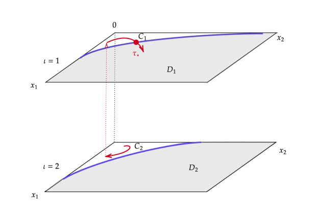
Figure 1: The optimal stopping time $\tau_{*}$ is the first entry time of $(\alpha,X)$ into $D$ at some point on the optimal stopping boundary in the first layer.

6 Quickest real-time detection of a Markovian drift

In this section, we apply this paper’s results to a quickest detection problem of a Brownian coordinate drift that was solved in the one-dimensional case in [14] and solved in the multidimensional case in [12], but now with random switching environments incorporated. Let $\alpha=\{\alpha_{t}:t\geq 0\}$ be a continuous time Markov chain with finite state space $M=\{1,\!\cdots\!,n\}$ and generator $Q=(q_{\iota\jmath})_{n\times n}$, i.e. for all $\iota\neq\jmath$, $\sum_{\jmath\in M}q_{\iota\jmath}=0$ and $q_{\iota\jmath}\geq 0$. As in [12, 14], we consider a Bayesian formulation of the quickest detection problem. That is, we assume that one observes a sample path of the standard two-dimensional Brownian motion $X=(X^{1},X^{2})$ with zero drift initially, and then at some random and unobservable time $\theta>0$ taking value $0$ with probability $\pi\in[0,1)$ and being exponentially distributed with parameter $\lambda>0$, one of the coordinate processes $X$ obtains a (known) non-zero drift $\mu$ permanently depending on the Markov chain. The aim is to detect the time $\theta$ as ‘accurately’ (to be specified below) as possible.

Based on the above formulation, the observed process $X=(X^{1},X^{2})$ solves the following stochastic differential equations

(6.1) $$dX^{i}_{t}=\mu(\alpha_{t})I(t\geq\theta,\beta=i)dt+dB^{i}_{t}\text{ for }i=1,2,$$

where $\beta$ denotes the number of the coordinate process which obtains the Markovian drift. We suppose that the prior distribution of $\beta$ is given with $\mathsf{P}(\beta=i)=p_{i}\geq 0$ with $p_{1}+p_{2}=1$. Further, the unobservable time $\theta$, the random variable $\beta$, and the driving Brownian motion $B$ are all assumed to be independent.

Being based upon the continuous observation of $(\alpha,X)$, the problem is to find a stopping time $\tau_{*}$ of $(\alpha,X)$, i.e. a stopping time with respect to the natural filtration ${\cal F}^{\alpha,X}_{t}=\sigma(\alpha_{s},X_{s}:0\leq s\leq t)$ augmented with all $\mathsf{P}$-null sets that is ‘as close as possible’ to the unknown time $\theta$. We formalize the phrase ‘as close as possible’ by introducing the following cost functional for the stopping time $\tau$

(6.2) $$J(\tau)=\mathsf{P}(\tau<\theta)+c\mathsf{E}\>\!\Big{[}F(\tau-\theta)I(\tau>\theta)\Big{]},$$

where $F(t):=e^{\gamma t}-1$ for a given $\gamma>0$. In the above equation, the first term corresponds to the probability of false alarm and the second term corresponds to expected exponentially penalized detection delay. Therefore, the value function of our quickest detection problem is equivalent to the minimization problem

(6.3) $$V=\inf_{\tau}J(\tau),$$

where the infimum is taken for all (bounded) stopping times of $(\alpha,X)$.

6.1 Measure change

In this section, we will reconstruct the stochastic process in (6.1) and the minimization problem in (6.3) on a new probability measure space where the quickest detection problem (6.3) can be reformulated as an optimal stopping problem through a suitable change of measure.

We begin by considering a probability measure space $(\Omega,{\cal F},\mathsf{P}^{0})$ supporting a two-dimensional Brownian motion $X$. This space shall also support a Markov Chain $\alpha$ with transition matrix $Q$ as given above, a random variable $\beta$ with $\mathsf{P}^{0}(\beta=i)=p_{i}$, and a random variable $\theta$ with $\mathsf{P}^{0}(\theta=0)=\pi$ and $\mathsf{P}^{0}(\theta>t)=(1-\pi)e^{-\lambda t}$ for $t>0$. Further, $X$, $\alpha$, $\beta$ and $\theta$ are all assumed independent under $\mathsf{P}^{0}$. Let the natural filtration of $(\alpha,X)$ be $\mathbb{F}$ and its augmentation by $\sigma(\theta,\beta)$ be $\mathbb{G}$ (i.e. $\mathbb{G}=\{{\cal G}_{t}\}_{t\geq 0}$ where ${\cal G}_{t}=\sigma(\theta,\beta,\{\alpha_{s},X_{s}:s\leq t\})$. Our first task is to construct a new probability measure $\mathsf{P}$ such that the probability measure of $(\alpha,X)$ under $\mathsf{P}$ coincides with the solution of (6.1).

We now proceed towards this end. Let

(6.4) $$Z_{t}:=\exp\Big{\{}\sum_{i=1}^{2}\Big{(}\int_{0}^{t}\mu(\alpha_{t})I(s\geq\theta,\beta=i)dX^{i}_{s}-\int_{0}^{t}\mu^{2}(\alpha_{t})I(s\geq\theta,\beta=i)ds\Big{)}\Big{\}}.$$

We now define a new probability measure $\mathsf{P}$ on $(\Omega,{\cal F})$ such that, for every $t\geq 0$,

$$\frac{d\mathsf{P}}{d\mathsf{P}^{0}}\Big{|}_{{\cal G}_{t}}=Z_{t},$$

and where ${\cal F}=\sigma({\cal G}_{t}:t\geq 0)$. By Girsanov’s theorem, under the measure $\mathsf{P}$,

$$X_{t}-\vec{\mu}(t;\alpha,\beta,\theta)$$

is a two-dimensional standard Brownian motion, where

$$\vec{\mu}(t;\alpha,\beta,\theta):=\begin{pmatrix}\displaystyle\int_{0}^{t}\mu(\alpha_{s})I(s\geq\theta,\beta=1)ds\\ \vskip 3.0pt plus 1.0pt minus 1.0pt\cr\displaystyle\int_{0}^{t}\mu(\alpha_{s})I(s\geq\theta,\beta=2)ds\end{pmatrix}.$$

Since $Z_{0}=1$, $\mathsf{P}$ and $\mathsf{P}^{0}$ coincide on ${\cal G}_{0}=\sigma(\beta,\theta)$, i.e. the distributions of $\theta$ and $\beta$ under $\mathsf{P}^{0}$ and $\mathsf{P}$ are the same. For the new measure $\mathsf{P}$, given the initial value $\alpha_{0}=\iota$ and the constant $\pi$, the cost function $J$ can be represented as

(6.5) $$\begin{array}[]{ll}J(\tau;\iota,\pi)&\!\!\!\displaystyle=\mathsf{P}^{0}(\tau<\theta)+c\mathsf{E}\>\!^{0}\Big{[}F(\tau-\theta)I(\tau>\theta)\Big{]}\\ \vskip 3.0pt plus 1.0pt minus 1.0pt\cr&\!\!\!\displaystyle=\sum_{i=1}^{2}p_{i}\Big{(}\mathsf{P}^{0}_{i}(\tau<\theta)+c\mathsf{E}\>\!^{0}_{i}\big{[}F(\tau-\theta)I(\tau>\theta)\big{]}\Big{)},\end{array}$$

where $\mathsf{P}_{i}$ is the probability measure under $\mathsf{P}$ given $\beta=i$. We now reformulate the problem using the measure $\mathsf{P}^{0}$.

To tackle (6.5), we consider the posterior probability distribution process $\varPi_{t}=(\varPi^{1}_{t},\varPi^{2}_{t})$ and the corresponding weighted likelihood ratio process $(\varPhi,\varPsi)$ given the data $(\alpha,X)$ observed up until time $t$, where the aforementioned quantities are defined as

(6.6) $$\left\{\begin{array}[]{ll}&\!\!\!\displaystyle\varPi^{i}_{t}:=\mathsf{P}^{0}_{i}(\theta\leq t|{\cal F}_{t}^{\alpha,X}),\text{ for }i=1,2,\\ \vskip 3.0pt plus 1.0pt minus 1.0pt\cr&\!\!\!\displaystyle\varPhi_{t}:=\frac{\mathsf{E}\>\!^{0}_{1}\big{[}e^{\gamma(t-\theta)}I(\theta\leq t)\big{|}{\cal F}_{t}^{\alpha,X}\big{]}}{1-\varPi^{1}_{t}},\\ \vskip 3.0pt plus 1.0pt minus 1.0pt\cr&\!\!\!\displaystyle\varPsi_{t}:=\frac{\mathsf{E}\>\!^{0}_{2}\big{[}e^{\gamma(t-\theta)}I(\theta\leq t)\big{|}{\cal F}_{t}^{\alpha,X}\big{]}}{1-\varPi^{2}_{t}}\end{array}\right.$$

where ${\cal F}^{\alpha,X}$ is the natural filtration of $(\alpha,X)$ augmented with all $\mathsf{P}^{0}$-null sets. By Girsanov’s theorem,

$$\frac{d\mathsf{P}_{i}}{d\mathsf{P}_{i}^{0}}\Big{|}_{{\cal G}_{t}}=Z^{i}_{t},$$

where $(Z^{1},Z^{2})$ is defined by

(6.7) $$Z^{i}_{t}:=\exp\Big{\{}\int_{0}^{t}\mu(\alpha_{s})I(s\geq\theta)dX^{i}_{s}-\frac{1}{2}\int_{0}^{t}\mu^{2}(\alpha_{s})I(s\geq\theta)ds\Big{\}}.$$

We now wish to use $(\varPhi,\varPsi)$ to represent the cost functional $J$ under the measure $\mathsf{P}$. Under the measure $\mathsf{P}$, for $\tau<\theta$, $Z^{i}_{\theta}=1$ almost surely. It then follows that

(6.8) $$\mathsf{P}^{0}_{i}(\tau<\theta)=\mathsf{E}\>\!_{i}^{0}(Z^{i}_{\theta}I(\tau<\theta))=\mathsf{P}_{i}(\tau<\theta)=1-\pi-(1-\pi)\mathsf{E}\>\!_{i}\int_{0}^{\tau}\lambda e^{-\lambda t}dt.$$

Using the formula for conditional probability, we obtain

$$\begin{array}[]{ll}&\!\!\!\displaystyle 1-\varPi^{i}_{t}=\mathsf{P}^{0}_{i}(\theta>t|{\cal F}_{t}^{\alpha,X})=\frac{\mathsf{E}\>\!_{i}[Z^{i}_{t}I(t<\theta)|{\cal F}_{t}^{\alpha,X}]}{\mathsf{E}\>\!_{i}[Z^{i}_{t}|{\cal F}_{t}^{\alpha,X}]}=\frac{(1-\pi)e^{-\lambda t}}{\mathsf{E}\>\!_{i}[Z^{i}_{t}|{\cal F}_{t}^{\alpha,X}]},\end{array}$$

where in the second equality we have employed the assumption that $X$, $\alpha$, $\beta$ and $\theta$ are independent under $\mathsf{P}^{0}$ and recalled that $Z_{t}^{i}=1$ almost surely on $\{t\leq\theta\}$. We continue by calculating

(6.9) $$\begin{array}[]{ll}\varPhi_{t}&\!\!\!\displaystyle=\frac{\mathsf{E}\>\!^{0}_{1}\big{[}e^{\gamma(t-\theta)}I(\theta\leq t)\big{|}{\cal F}_{t}^{\alpha,X}\big{]}}{1-\varPi^{1}_{t}}\\ \vskip 3.0pt plus 1.0pt minus 1.0pt\cr&\!\!\!\displaystyle=\frac{\mathsf{E}\>\!_{1}\big{[}Z^{1}_{t}e^{\gamma(t-\theta)}I(\theta\leq t)\big{|}{\cal F}_{t}^{\alpha,X}\big{]}}{(1-\varPi^{1}_{t})\mathsf{E}\>\!_{1}[Z^{1}_{t}|{\cal F}_{t}^{\alpha,X}]}=\frac{\mathsf{E}\>\!_{1}\big{[}Z^{1}_{t}e^{\gamma(t-\theta)}I(\theta\leq t)\big{|}{\cal F}_{t}^{\alpha,X}\big{]}}{(1-\pi)e^{-\lambda t}}.\end{array}$$

Further,

(6.10) $$\begin{array}[]{ll}&\!\!\!\displaystyle\mathsf{E}\>\!^{0}_{1}\Big{[}F(\tau-\theta)I(\tau>\theta)\Big{]}=\gamma\mathsf{E}\>\!^{0}_{1}\Big{[}I(\tau>\theta)\int_{\theta}^{\tau}e^{\gamma(s-\theta)}ds\Big{]}\\ \vskip 3.0pt plus 1.0pt minus 1.0pt\cr&\!\!\!\displaystyle=\gamma\mathsf{E}\>\!^{0}_{1}\Big{[}\int_{0}^{\infty}I(t\geq\theta)I(t<\tau)e^{\gamma(s-\theta)}dt\Big{]}\\ \vskip 3.0pt plus 1.0pt minus 1.0pt\cr&\!\!\!\displaystyle=\gamma\mathsf{E}\>\!_{1}\Big{[}\int_{0}^{\infty}Z^{1}_{t}I(t\geq\theta)I(t<\tau)e^{\gamma(t-\theta)}dt\Big{]}\\ \vskip 3.0pt plus 1.0pt minus 1.0pt\cr&\!\!\!\displaystyle=\gamma\mathsf{E}\>\!_{1}\left\{\int_{0}^{\infty}I(t<\tau)\mathsf{E}\>\!_{1}\Big{[}Z^{1}_{t}I(t\geq\theta)e^{\gamma(t-\theta)}\Big{|}{\cal F}_{t}^{\alpha,X}\Big{]}dt\right\}\\ \vskip 3.0pt plus 1.0pt minus 1.0pt\cr&\!\!\!\displaystyle=(1-\pi)\gamma\mathsf{E}\>\!_{1}\int_{0}^{\tau}e^{-\lambda t}\varPhi_{t}dt.\end{array}$$

Similarly, we may conclude that

(6.11) $$\begin{array}[]{ll}&\!\!\!\displaystyle\mathsf{E}\>\!^{0}_{2}\Big{[}F(\tau-\theta)I(\tau>\theta)\Big{]}=(1-\pi)\gamma\mathsf{E}\>\!_{2}\int_{0}^{\tau}e^{-\lambda t}\varPsi_{t}dt.\end{array}$$

Together with (6.8), (6.10) and (6.11), (6.2) implies that

(6.12) $$J(\tau;\iota,\pi)=1-\pi+c\gamma(1-\pi)\mathsf{E}\>\!_{\iota,\frac{\pi}{1-\pi},\frac{\pi}{1-\pi}}\int_{0}^{\tau}e^{-\lambda t}\Big{(}p_{1}\varPhi_{t}+p_{2}\varPsi_{t}-\frac{\lambda}{c\gamma}\Big{)}dt,$$

where subscript under $\mathsf{E}\>\!$ denotes the initial data of $(\alpha,\varPhi,\varPsi)$.
We now derive the stochastic differential equation for $(\varPhi,\varPsi)$ under the measure $\mathsf{P}$. We write the likelihood ratio process as

(6.13) $$L^{i}_{t}:=\exp\Big{\{}\int_{0}^{t}\mu(\alpha_{s})dX^{i}_{s}-\frac{1}{2}\int_{0}^{t}\mu^{2}(\alpha_{s})ds\Big{\}}.$$

It can now be easily seen from (6.7) that

$$Z_{t}^{i}=I(t<\theta)+\frac{L^{i}_{t}}{L^{i}_{\theta}}I(t\geq\theta).$$

Invoking the assumption that $X$, $\alpha$, $\theta$ and $\beta$ are independent under $\mathsf{P}^{0}$, we see from (6.9) that

(6.14) $$\varPhi_{t}=\frac{e^{\lambda t}}{(1-\pi)}\mathsf{E}\>\!_{1}\big{[}Z^{1}_{t}e^{\gamma(t-\theta)}I(\theta\leq t)\big{|}{\cal F}_{t}^{\alpha,X}\big{]}=e^{(\lambda+\gamma)t}L^{1}_{t}\Big{(}\frac{\pi}{1-\pi}+\int_{0}^{t}\frac{\lambda e^{-(\lambda+\gamma)s}}{L^{1}_{s}}ds\Big{)}.$$

Similarly, we have that

(6.15) $$\varPsi_{t}=e^{(\lambda+\gamma)t}L^{2}_{t}\Big{(}\frac{\pi}{1-\pi}+\int_{0}^{t}\frac{\lambda e^{-(\lambda+\gamma)s}}{L^{2}_{s}}ds\Big{)}.$$

Under the measure $\mathsf{P}$, $\widehat{B}_{t}=X_{t}$ is standard Brownian motion and $dL^{i}_{t}=\mu(\alpha_{t})L^{i}_{t}dX^{i}_{t}$. Therefore, under the measure $\mathsf{P}$, the couple $(\varPhi,\varPsi)$ solves the following system of stochastic differential equations with Markov switching

(6.16) $$\left\{\begin{array}[]{ll}&\!\!\!\displaystyle d\varPhi_{t}=[\lambda+(\lambda+\gamma)\varPhi_{t}]dt+\mu(\alpha_{t})\varPhi_{t}d\widehat{B}^{1}_{t}\\ \vskip 3.0pt plus 1.0pt minus 1.0pt\cr&\!\!\!\displaystyle d\varPsi_{t}=[\lambda+(\lambda+\gamma)\varPsi_{t}]dt+\mu(\alpha_{t})\varPsi_{t}d\widehat{B}^{2}_{t}.\end{array}\right.$$

From (6.7), (6.14), and (6.15), $(\alpha,\varPhi,\varPsi)$ is observable in real time, and these are the sufficient statistics for our quickest detection problem.

We now offer an equivalent formulation of our quickest detection problem as the following optimal stopping problem

(6.17) $$\widehat{V}(\iota,\varphi,\psi)=\inf_{\tau}\mathsf{E}\>\!_{\iota,\varphi,\psi}\int_{0}^{\tau}e^{-\lambda t}\Big{(}p_{1}\varPhi_{t}+p_{2}\varPsi_{t}-\frac{\lambda}{c\gamma}\Big{)}dt,$$

where the infimum is taken over for all stopping times of $(\alpha,\varPhi,\varPsi)$ solving the system of equations in (6.16). The value function may then be represented as

(6.18) $$V(\iota,\pi)=(1-\pi)\left(1+c\gamma\widehat{V}\left(\iota,\frac{\pi}{1-\pi},\frac{\pi}{1-\pi}\right)\right).$$

In order to apply the results in the present paper to this problem, we need only verify that Assumptions 2.1, 2.2 and 2.3 from Section 2 hold for the optimal stopping problem in (6.17). Indeed, in the present problem, we have that $a^{i}(\iota)=\lambda$, $b^{ii}(\iota)=\lambda+\gamma$, $b^{ij}(\iota)=0$ if $i\neq j$, $\sigma^{i}(\iota)=\mu(\iota)$, $\lambda(\iota)=\lambda$ and

$$H(\iota,\varphi,\psi)=p_{1}\varphi+p_{2}\psi-\frac{\lambda}{c\gamma}.$$

This verifies Assumptions 2.1, 2.2, and 2.3. Combining Theorem 3.8 and Theorem 5.1, we disclose in Corollary 6.1 below the key result for the real-time quickest detection problem with switching states.

Corollary 6.1.

Given $\pi\in[0,1)$, $\lambda,\gamma,\mu(\cdot)>0$ and $p_{1},p_{2}\geq 0$ with $p_{1}+p_{2}\!=\!1$, the quickest detection problem given in (6.3) admits the following representation

$$V(\iota,\pi)=(1-\pi)\Big{[}1+c\gamma\widehat{V}\Big{(}\iota,\frac{\pi}{1-\pi},\frac{\pi}{1-\pi}\Big{)}\Big{]},$$

where $\widehat{V}$ is given by (6.17) above. The optimal stopping time is given by

$$\begin{array}[]{ll}\displaystyle\tau^{*}&\!\!\!\displaystyle=\inf\Big{\{}t\geq 0:\varPsi_{t}\geq b_{\alpha_{t}}(\varPhi_{t})\Big{\}},\end{array}$$

where the sufficient statistics $(\alpha,\varPhi,\varPsi)$ are given by

$$\left\{\begin{array}[]{ll}&\!\!\!\displaystyle L^{i}_{t}=\exp\Big{\{}\int_{0}^{t}\mu(\alpha_{s})dX^{i}_{s}-\frac{1}{2}\int_{0}^{t}\mu^{2}(\alpha_{s})ds\Big{\}}\text{ for }i=1,2;\\ \vskip 3.0pt plus 1.0pt minus 1.0pt\cr&\!\!\!\displaystyle\varPhi_{t}=e^{(\lambda+\gamma)t}L^{1}_{t}\Big{(}\frac{\pi}{1-\pi}+\lambda\int_{0}^{t}\frac{1}{e^{(\lambda+\gamma)s}L^{1}_{s}}ds\Big{)};\\ \vskip 3.0pt plus 1.0pt minus 1.0pt\cr&\!\!\!\displaystyle\varPsi_{t}=e^{(\lambda+\gamma)t}L^{2}_{t}\Big{(}\frac{\pi}{1-\pi}+\lambda\int_{0}^{t}\frac{1}{e^{(\lambda+\gamma)s}L^{2}_{s}}ds\Big{)},\end{array}\right.$$

where $\alpha$ is a Markov chain with initial state $\alpha_{0}=\iota$ and $\{b_{\iota}\}_{\iota\in M}$ is the unique solution to (5.1) in the admissible class given in Theorem 5.1.

Acknowledgements The first-named author is grateful to ARO-YIP-71636-MA, NSF DMS-1811936, ONR N00014-18-1-2192, and ONR N00014-21-1-2672 for their support of this research.

References

• [1]
• [2] Applebaum, D. (2009). Lévy Processes and Stochastic Calculus. Cambridge University Press.
• [3] Borwein, J.M. and Vanderwerff, J.D. (2010). Convex Functions: Constructions, Characterizations and Counterexamples. Cambridge University Press.
• [4] Christensen, S., Crocce, F., Mordecki, E., and Salminen, P. (2019). On optimal stopping of multidimensional diffusions. Stochastic Processes and their Applications, 129(7), (2561–2581).
• [5] Chung, K.L. (2013). Lectures from Markov Processes to Brownian Motion (Vol. 249). Springer Science & Business Media.
• [6] Dai, S. and Menoukeu-Pamen, O. (2018). Viscosity solution for optimal stopping problems of Feller processes. arXiv preprint arXiv:1803.03832.
• [7] Dayanik, S. (2008). Optimal stopping of linear diffusions with random discounting. Mathematics of Operations Research, 33(3), (645–661).
• [8] Dayanik, S. and Karatzas, I. (2003). On the optimal stopping problem for one-dimensional diffusions. Stochastic Processes and their Applications, 107(2), (173-–212).
• [9] De Angelis, T. and Peskir, G. (2020). Global $C^{1}$ regularity of the value function in optimal stopping problems. The Annals of Applied Probability, 30(3), (1007–1031).
• [10] Du Toit, J. and Peskir, G. (2009). Selling a stock at the ultimate maximum. The Annals of Applied Probability 19(3), (983–1014).
• [11] Eizenberg, A. and Freidlin, M. (1990). On the Dirichlet problem for a class of second order PDE systems with small parameter. Stochastics and Stochastic Reports, 33(3-4), (111–148).
• [12] Ernst, P.A. and Peskir, G. (2020). Quickest real-time detection of a Brownian coordinate drift. arXiv preprint arXiv:2007.14786.
• [13] Ferreyra, G., and Sundar, P. (2000). Comparison of solutions of stochastic equations and applications. Stochastic Analysis and Applications, 18(2), (211–229).
• [14] Gapeev, P.V. and Shiryaev, A.N. (2013). Bayesian quickest detection problems for some diffusion processes. Advances in Applied Probability 45(1), (164–185).
• [15] Gilbarg, D. and Trudinger, N.S. (2001). Elliptic Partial Differential Equations of the Second Order. Springer.
• [16] Jobert, A.and Rogers, L.C.G. (2006). Option pricing with Markov-modulated dynamics. SIAM Journal on Control and Optimization, 44(6), (2063–2078).
• [17] Karatzas, I. and Shreve, S.E. (1998). Brownian Motion and Stochastic Calculus. Springer, New York, NY.
• [18] Lamberton, D. and Zervos, M. (2013). On the optimal stopping of a one-dimensional diffusion. Electronic Journal of Probability, 18 (34), (1–49).
• [19] Liu, R.H. (2016). Optimal stopping of switching diffusions with state dependent switching rates. Stochastics, 88(4), (586–605).
• [20] McKean, H.P. (1965). A free boundary problem for the heat equation arising from a problem of mathematical economics. Industrial Management Review, 6, (32–39).
• [21] Peskir, G. (2007). A change-of-variable formula with local time on surfaces. Sém. de Probab. XL, Lecture Notes in Math. 1899, Springer (69–96).
• [22] Peskir, G. (2019). Continuity of the optimal stopping boundary for two-dimensional diffusions. The Annals of Applied Probability, 29(1), (505–530).
• [23] Peskir, G. and Shiryaev, A.N. (2006). Optimal Stopping and Free-Boundary Problems. Lectures in Mathematics, ETH Zürich, Birkhäuser.
• [24] Shiryaev, A.N. (2010). Quickest detection problems: Fifty years later. Sequential Analysis, 29(4), (345–385).
• [25] Yin, G. and Zhu, C. (2009). Hybrid Switching Diffusions: Properties and Applications (Vol. 63). Springer Science & Business Media.
• [26] Zhang, Q. and Guo, X. (2004). Closed-form solutions for perpetual American put options with regime switching. SIAM Journal on Applied Mathematics, 64(6), (2034–2049).
• [27] Zhang, Q., Yin, G., and Liu, R.H. (2005). A near-optimal selling rule for a two-time-scale market model. Multiscale Modeling & Simulation, 4(1), (172–193).