uiCA: Accurate Throughput Prediction of
Basic Blocks on Recent Intel Microarchitectures

Abstract.

Performance models that statically predict the steady-state throughput of basic blocks on particular microarchitectures, such as IACA, Ithemal, llvm-mca, OSACA, or CQA, can guide optimizing compilers and aid manual software optimization. However, their utility heavily depends on the accuracy of their predictions. The average error of existing models compared to measurements on the actual hardware has been shown to lie between 9% and 36%. But how good is this? To answer this question, we propose an extremely simple analytical throughput model that may serve as a baseline. Surprisingly, this model is already competitive with the state of the art, indicating that there is significant potential for improvement.

To explore this potential, we develop a simulation-based throughput predictor. To this end, we propose a detailed parametric pipeline model that supports all Intel Core microarchitecture generations released between 2011 and 2021. We evaluate our predictor on an improved version of the BHive benchmark suite and show that its predictions are usually within 1% of measurement results, improving upon prior models by roughly an order of magnitude. The experimental evaluation also demonstrates that several microarchitectural details considered to be rather insignificant in previous work, are in fact essential for accurate prediction.

Our throughput predictor is available as open source.

1. Introduction

Performance models are widely used to predict, understand, and optimize performance. Such models have been proposed at all kinds of abstraction levels, targeting different resources and applications. In this work, we are considering the problem of predicting the steady-state throughput of basic blocks, i.e., the number of processor clock cycles it takes to execute a basic block in steady state in a loop.

Being able to accurately predict basic-block throughput is important both for compiler designers and for performance engineers. Compiler optimizations, for instance, may rely on such performance models to apply auto-vectorization, register allocation, and instruction scheduling (mcgovern99, ; stephenson03, ; lozano12, ) in an informed manner. Performance engineers may use such models to pinpoint constraining bottlenecks, which can then be mitigated by code changes.

Clearly, the utility of such models depends greatly on the accuracy of their predictions. Both Pohl et al. (pohl19, ; pohl20, ) and Mendis and Amarasinghe (mendis18, ) observe that the inaccuracy of existing cost models often misguides optimizations at the cost of performance.

In recent work, several basic block performance analysis models have been proposed, such as IACA (iacaGuide, ), llvm-mca (dibiagio18, ; llvmmca, ), OSACA (Laukemann18, ; Laukemann19, ), CQA (cqa14, ), Ithemal (mendis19a, ), and DiffTune (Renda20, ). Chen et al. (Chen19, ) developed the BHive benchmark suite specifically to evaluate the accuracy of these models. They found that the average error of the predictions of existing tools compared to measurements on the actual hardware lies between 9% and 36%.

At the onset of this work, we were wondering how good an accuracy in this range actually is. To shed light on this question, we first developed the following simple analytical throughput predictor that can serve as a baseline. We predict the throughput of a benchmark on the Skylake microarchitecture as

$$TP_{\textit{baseline}}=max\left(\frac{n}{4},\frac{m_{r}}{2},m_{w}\right),$$

where $n$ is the number of instructions, $m_{r}$ the number of memory reads, and $m_{w}$ the number of memory writes of the benchmark. Note that Skylake has four decoders, and it can perform two memory reads and one memory write per cycle. Thus, the three constituents of the formula directly follow from basic throughput limits of the microarchitecture.

Table 1 shows the mean absolute percentage error (MAPE) and Kendall’s tau coefficient (for details see Section 6) of the predictions of different tools relative to the reference measurements that were published along with the BHive benchmark suite (Chen19, ) for the Skylake microarchitecture. Surprisingly, our simple baseline predictor achieves an average error of around 17%, which is better than several previous approaches that are significantly more complex.

Table 1. State of the art in basic-block throughput prediction

Predictor	MAPE	Kendall’s Tau
Ithemal	9.51%	0.8523
IACA 3.0	14.50%	0.8131
DiffTune	24.62%	0.7444
llvm-mca-10	27.91%	0.7832
OSACA	29.74%	0.7770
Baseline	17.21%	0.7719

This yields the following questions that we address in this work:

1. What are the reasons for the discrepancies between the predictions of existing models and measurements?

2. How can these discrepancies be eliminated?

We have identified two main issues that explain the discrepancies between measurements and predictions:

1. The microarchitectural models of previous tools are not detailed enough.

2. The experimental evaluations include unsuitable benchmarks, and are partly based on biased and inaccurate throughput measurements, and on incompatible throughput definitions.

To address the first issue, we develop a pipeline model that is significantly more detailed than prior models. It is applicable to all Intel Core microarchitectures released in the last decade. Still, the differences between these microarchitectures can be captured by a small number of parameters. A challenge in building such a model is that many of the relevant properties are undocumented. We have developed microbenchmark-based techniques to reverse-engineer these properties. Based on this model, we implement a simulator called uiCA (“uops.info Code Analyzer”) that predicts the throughput of basic blocks (Section 4).

To address the second issue, and to evaluate uiCA, we first identify two variants of the throughput prediction problem (Section 3) that capture differing assumptions in the existing models. Then we propose several improvements to the BHive benchmark suite that enable a fairer comparison of different tools. Finally, we develop a more accurate measurement methodology that supports both problem variants (Section 5).

Using this improved benchmark suite and measurement methodology, we compare uiCA with the existing tools on nine different Intel Core microarchitectures. uiCA’s predictions are usually within 1% of the measurement results, which improves upon the state of the art by roughly an order of magnitude (Section 6).

To summarize, the main contributions of our paper are:

• A parametric pipeline model that is applicable to all Intel Core microarchitectures from Sandy Bridge (2011) to Rocket Lake (2021) (Section 4).

• A throughput predictor (Section 4.3) based on this parametric model that is more accurate than previous work, often by more than an order of magnitude (Section 6).

• An improved set of benchmarks for validating throughput predictors, and a more accurate measurement methodology (Section 5).

2. Related Work

2.1. Models for Performance Prediction

Existing basic-block throughput models roughly fall into three camps: (1) simulation-based models, (2) analytical models, and (3) machine-learning-based models.

The Intel Architecture Code Analyzer (IACA) (iacaGuide, ) is a tool developed by Intel that can statically analyze the performance of loop kernels on several older microarchitectures. The tool generates a report which includes throughput and port usage data of the analyzed loop kernel. As the tool is closed source, its underlying model and prediction methodology are unknown. In April 2019, Intel announced IACA’s end of life.

The Open Source Architecture Code Analyzer (OSACA) (Laukemann18, ; Laukemann19, ) is an analytical performance prediction tool for Intel, AMD, and ARM microarchitectures. It is based on a relatively coarse-grained model of these microarchitectures; according to (Laukemann19, ), “accurately modeling the performance characteristics of the decode, reorder buffer, register allocation/renaming, retirement and other stages, which all may limit the execution throughput and impose latency penalties, is currently out of scope for OSACA.”

The LLVM Machine Code Analyzer (llvm-mca) (llvmmca, ) is a simulation-based tool that predicts the performance of machine code using scheduling models available in the LLVM compiler (llvm04, ). It supports processors for which a scheduling model is available in LLVM. llvm-mca does not model performance bottlenecks in the front end. It also does not model techniques such as micro/macro fusion or move elimination.

Within the MAQAO (maqao, ) framework, two performance analysis tools have been proposed: CQA (cqa14, ) and UFS (Palomares16, ). The Code Quality Analyzer (CQA) is a simulation-based tool that analyzes the performance of innermost loops. In addition to computing throughput predictions, it provides high-level code quality metrics like the vectorization ratio. CQA uses a front-end model that is more detailed than those of most other previous tools; however, it does not model the core of the execution engine “because of its complexity and lack of documentation.” UFS is a throughput predictor that uses a relatively detailed model of the back end of the Sandy Bridge microarchitecture, but only a very coarse-grained model of its front end. UFS exists only as a prototype that is not publicly available.

Ithemal (mendis19a, ) is a basic-block throughput predictor that is based on a deep neural network. This neural network has been trained using training data obtained from measurements on the actual hardware. This data-driven approach holds the promise of alleviating the tedious modeling effort required to build conventional simulators. Unlike most of the other tools discussed in this section, it predicts a basic block’s throughput but does not provide other insights into how the code is executed, which may be useful for performance engineers. To obtain a more interpretable model, Renda et al. present DiffTune (Renda20, ), an approach that applies machine learning to obtain the microarchitecture-specific parameters for the x86 simulation model used by llvm-mca. As it is based on llvm-mca, it shares its modeling limitations. Both Ithemal and DiffTune were trained on measurements performed with a profiling tool by Chen et al. (Chen19, ). In contrast to previous tools, this tool can automatically profile basic blocks that may perform arbitrary memory accesses. We build upon this tool in Section 5.3.

Full-system simulators (austin02, ; yourst07, ; loh09, ; binkert11, ; patel11, ; sanchez13, ) such as ZSim or gem5 can simulate the execution of entire programs, modeling the interactions between different hardware components including deep memory hierarchies and multi-core architectures. In contrast to basic-block throughput predictors, full-system simulators require a program’s input data to drive the simulation. In principle, the pipeline model developed in this paper could be integrated into full-system simulators to improve their accuracy.

2.2. Microbenchmarking

One approach to construct detailed performance models is to reverse engineer the relevant parameters by microbenchmarking.

Agner Fog (fogTest, ) provides a measurement tool and a set of test scripts that generate microbenchmarks to analyze various properties of microarchitectures. He maintains a set of tables with instruction latencies, throughputs and micro-operation breakdowns (fog21, ), as well as a document with detailed descriptions of many recent microarchitectures (fog21uArch, ).

nanoBench (Abel20, ; Abel20b, ) is a tool for evaluating small microbenchmarks on x86 systems using hardware performance counters. nanoBench is used to evaluate the microbenchmarks for obtaining the latency, throughput, and port usage data that is available at uops.info (Abel19, ), which we extend in this work and employ in our tool.

PMEvo (Ritter20, ) is a framework by Ritter and Hack that can automatically infer port mappings based on measured execution times of short code sequences. A related approach that also takes into account other limiting resources besides execution ports was recently proposed by Derumigny et al. (derumigny22, ). The models obtained by these two approaches may be used to predict the throughput of dependency-free basic blocks.

3. Basic-Block Throughput Prediction

In this section, we state more precisely the problem basic-block throughput predictors aim to solve.

3.1. Notions of Throughput

The throughput of a basic block is commonly defined as the average number of clock cycles per iteration when executing the basic block repeatedly in a steady state.

However, “executing the basic block repeatedly” can mean different things, depending on the type of basic block that is used.

For basic blocks that end in a branch instruction that jumps back to the beginning of the block, “executing the basic block repeatedly” can reasonably be interpreted to mean executing the block in a way that the branch is always taken; this corresponds to executing the basic block as an infinite loop. In the following, we will refer to this notion of throughput as $TP_{L}$.

Basic blocks that do not end in a branch instruction cannot be executed in this way. For such blocks, a way to “execute the basic block repeatedly” is to unroll the basic block a sufficient number of times to reach a steady state. In the following, we will refer to this notion of throughput as $TP_{U}$.

An important difference between the two notions is that for $TP_{L}$, the µops of many benchmarks are delivered by the µOP cache (DSB) or the loop stream detector (see Section 4), whereas for $TP_{U}$, all µops have to go through the decoders, which can be significantly slower. As an example, consider the basic block

ADD AX, 0x1234; DEC R15

When unrolling this code sequence multiple times, the average execution time on a Skylake CPU is $3.44$ cycles per iteration; the bottleneck here is a stall in the predecoder. On the other hand, the code sequence

loop: ADD AX, 0x1234; DEC R15; JNZ loop

is served from the µOP cache (DSB) and requires, on average, only one cycle per loop iteration, even though it has an additional instruction.

Previous work did not clearly distinguish the two throughput notions. Intel’s IACA treats the basic block as the “body of an infinite loop”. Thus, it is based on $TP_{L}$. Correspondingly, all examples in IACA’s user guide (iacaGuide, ) are basic blocks that end in a branch instruction that jumps back to the beginning of the block. IACA does not reject basic blocks that are not of this form; however, the behavior in such a case is not specified in the documentation. Chen et al. claim to use “IACA’s definition of throughput” (Chen19, ). However, their measurement framework only considers basic blocks that do not end in a branch instruction. They measure the throughput by unrolling; thus their notion of throughput actually corresponds to $TP_{U}$.

OSACA (Laukemann18, ; Laukemann19, ) and CQA (cqa14, ) are based on $TP_{L}$; CQA can only analyze code that ends in a branch instruction. For llvm-mca, it is not completely clear which definition is used. According to the documentation, llvm-mca “simulates the execution of the machine code sequence in a loop of iterations” (llvmmca, ); however, the examples in the documentation do not end in a branch instruction. As llvm-mca does not model performance bottlenecks in the front end, the throughput predictions can generally be expected to be closer to measurements based on the $TP_{L}$ notion.

In this work, we develop a throughput predictor that can predict the throughput under both notions. For basic blocks that end in a branch instruction, we use $TP_{L}$; for other blocks, we use $TP_{U}$.

3.2. Common Modeling Assumptions

A common and sometimes unstated assumption is that basic-block throughput predictors are intended to statically analyze the performance of compute-bound basic blocks, i.e., basic blocks whose throughput is not memory- or I/O-bound. A basic-block throughput predictor may be one component of tools and methodologies to determine whether code is actually compute bound, such as the Roofline model (williams09, ) or the Execution-Cache-Memory model (Stengel15, ; hammer17, ); however, determining compute-boundedness is not in scope for basic-block throughput predictors themselves.

Further modeling assumptions arise from the fact that basic blocks are analyzed statically without knowledge of the state of the execution environment, such as the values of registers, memory, or microarchitectural components such as branch predictors.

We summarize these common modeling assumptions in the following:

• All memory accesses are executed optimally. This means there are no cache or TLB misses, no unaligned loads, no bank conflicts (intelOptManual20, ; Jiang17, ), and stores can always be paired (intelOptManual20, ).

• There are no branch mispredictions.

• The basic blocks were emitted by a compiler or written by a reasonably competent, non-adversarial programmer. Thus, they do not contain corner cases that would not occur in realistic, performance-critical code like undefined instructions, x87 floating-point stack underflows or overflows, or memory accesses to invalid addresses.

• There are no denormal floating-point operations.

• There are no operations that lead to exceptions, and no interrupts occur during the execution.

• A problematic class of basic blocks for static throughput predictors are blocks with input-dependent timing. This includes blocks that use variable-latency instructions, and blocks for which it depends on the inputs whether two memory accesses alias. Most existing tools optimistically assume that the inputs are such that no memory aliasing occurs; in llvm-mca it can be configured via a parameter whether such memory accesses are assumed to alias or not. For variable-latency instructions, the behavior of existing tools is inconsistent. For divisions, most tools yield pessimistic predictions; for the cpuid instruction, on the other hand, the predictions are typically optimistic.

It should be noted that for actual programs, these assumptions do not necessarily hold. However, techniques to check whether the assumptions hold are mostly orthogonal to the techniques required for basic-block throughput prediction, and it makes therefore sense to separate these concerns.

4. A Parametric Pipeline Model

Figure 1 shows the general structure of the pipelines of recent Intel Core CPUs. At such a high level, all these CPUs are very similar. For developing an accurate performance predictor, however, a more detailed model is necessary.

In this section, we describe the parametric pipeline model that we have developed. First, in Section 4.1, we describe the different pipeline components of recent Intel CPUs. Then, in Section 4.2, we look at properties of how individual instructions are executed. Finally, in Section 4.3, we discuss how the model is used to implement a throughput predictor.

Many of the details that are necessary to build such a detailed model are undocumented. We have reverse-engineered these details via microbenchmarks using hardware performance counters. For evaluating these microbenchmarks, we use nanoBench (Abel20, ) and an extension to nanoBench that provides cycle-by-cycle performance data, similar to Brandon Falk’s “Sushi Roll” approach (Falk19, ). Due to space constraints, we are unable to describe these microbenchmarks in this section; we will describe those in a separate technical report. Instead, we will only describe our findings. We highlight the corresponding paragraphs with a blue bar on the left.

The model presented in this section is significantly more detailed than all previous models described in the literature. It is applicable to all Intel Core microarchitectures from Sandy Bridge to Rocket Lake. We found that, maybe surprisingly, the differences between these microarchitectures that are relevant for our work can be captured by a relatively small number of parameters. We mark the paragraphs that describe these parameters with a red bar on the right.

4.1. Pipeline Properties

4.1.1. Front End

The predecoder fetches aligned 16-byte blocks from the instruction cache (at most one such block per cycle), and it is mainly responsible for detecting where each instruction begins. This is not completely straightforward, as an instruction can be between 1 and 15 bytes long, and detecting its length can require inspecting several bytes of the instruction. The predecoded instructions are inserted into the instruction queue (IQ).

Figure 1. Pipeline of Intel Core CPUs

According to our experiments, the predecoder can predecode at most five instructions per cycle. If there are, e.g., six instructions in a 16-byte block, in the first cycle, five instructions would be predecoded, and in the next cycle, only one instruction would be predecoded. Several sources incorrectly claim that the predecoding limit is six instructions per cycle (Schaik19, ; wikichipSkylake, ; realworldtechHaswell, ; ren21, ); the source for this might be a section in Intel’s optimization manual (intelOptManual20, ) that mentions such a limit; however, this section only applies to old Intel Core 2 CPUs, which did not have a µop cache, and thus decoding was a more significant bottleneck.

A special case are instructions with a so called length-changing prefix (LCP). For such instructions, the predecoder has to use a slower length-decoding algorithm. This results in a penalty of three cycles for each such instruction.

For building an accurate simulator, it is important to know how instructions that cross a 16-byte boundary are predecoded; however, this is undocumented. Our experiments show that instructions are predecoded with the 16-byte block in which they end; they count toward the limit of five instructions in the corresponding cycle. We found that there is a one cycle penalty if five instructions were predecoded in the current cycle, the next instruction crosses a 16-byte boundary, but the primary opcode is contained in the current 16-byte block; if there are only prefixes or escape opcodes of the next instruction in the current block, there is no penalty.

The decoding unit fetches up to four instructions per cycle from the IQ. It decodes the instructions into a sequence of µops and sends them to the Instruction Decode Queue (IDQ).

The decoding unit consists of one complex decoder and three simple decoders. The simple decoders can only decode instructions with a single µop. The complex decoder always decodes the first of the fetched instructions, and it can generate up to four µops. Several sources (e.g., (Schaik19, ; wikichipSkylake, ; anandtechSkylake, ; deng22, )) incorrectly claim that with the Skylake microarchitecture, the number of simple decoders was increased from three to four; this might be based on a misinterpretation of the fact that with Skylake, the number of µops that can be delivered from the decoding unit to the IDQ was increased from four to five.

Instructions with more than four µops are (at least partially) handled by the Microcode Sequencer (MS). We discovered that there are instructions that have only one µop but that can only be handled by the complex decoder.

The sizes of the IQ and the IDQ, whether a macro-fusible instruction can be decoded on the last decoder or when the instruction queue is empty, whether pop instructions require the complex decoder if registers rsp or r12 are used, and whether any other instructions can be decoded in the same cycle are parameters of our model.

Decoded µops are also stored in the Decoded Stream Buffer (DSB, also: µOP cache), subject to certain conditions. This can allow for a higher throughput of loops for which decoding is the bottleneck.

A cache line in the DSB of a pre-Ice Lake CPUs can store at most six µops that need to be contained in the same 32-byte aligned code block. There can be at most three cache lines that contain µops from a specific 32-byte block. If a 32-byte block contains more than three cache lines, no µop of this block will be stored in the DSB. There are a number of other restrictions; e.g., some µops require two slots in a cache line. These restrictions are not described in the official manuals, but they have been reverse engineered by Agner Fog (fog21uArch, ).

We have discovered that on Skylake and Cascade Lake CPUs, µops from a specific 32-byte block are only served from the DSB if both 32-byte blocks of the corresponding 64-byte instruction cache line fulfill the restrictions described in the previous paragraph.

Starting with the Ice Lake microarchitecture, the DSB operates on 64-byte blocks. There can be at most six cache lines (with up to six µops each) from a specific 64-byte block.

As a workaround for the “Jump Conditional Code” (JCC) erratum, Skylake-based CPUs with a recent microcode cannot cache blocks that contain a jump instruction that crosses or ends on a 32-byte boundary (jccErratum, ).

According to (fog21uArch, ), the “pipeline switches frequently between taking µops from the decoders and from the µop cache”. We have found out that a switch from the decoders to the DSB can only take place after a branch instruction. Thus, for loops that contain only one branch instruction at the end, a switch to the DSB can only take place at the start of a loop iteration.

We discovered that when switching from the decoders to the MS and back, there are two stall cycles (in total). Switching from the DSB to the MS and back incurs two stall cycles on Skylake and its successors, and four stall cycles on earlier microarchitectures; this contradicts (fog21uArch, ), which claims that “each switch may cost one clock cycle” on Sandy Bridge and Ivy Bridge.

The block size of the DSB, the maximum number of µops that the DSB can deliver per cycle, whether a 32 byte block can only be in the DSB if the other 32 byte block in the same 64 byte block is also cacheable, the number of stall cycles when switching from DSB to MS, and whether a branch instruction can be the last instruction in a block that is cached by the DSB are parameters of our model.

The Loop Stream Detector (LSD) detects loops whose µops fit entirely into the IDQ. In this case, it locks the µops in the IDQ, and streams them continuously without requiring the DSB or the decoders. The first µop of a loop iteration cannot be streamed in the same cycle as the last µop of the previous iteration. As this could be a significant bottleneck for small loops, the LSD can automatically unroll the loop. While this unrolling is briefly mentioned in the manual, no details are provided.

We have reverse engineered how often the LSD unroll loops of different sizes on different microarchitectures.

Whether the LSD is enabled (on Skylake-based CPUs, it was disabled with a microcode update due to the SKL150 erratum (sklSpecUpdate, )), and how the code is unrolled by the LSD, are parameters of our model.

4.1.2. Renamer / Allocator

The renamer (also called Resource Allocation Table (RAT)) maps architectural registers to physical registers. It also allocates resources for loads and stores, and it assigns execution ports to the µops.

The renamer fetches µops from the IDQ. It stores all µops in the reorder buffer, and it issues them to the scheduler (see Section 4.1.3). We call the maximum number of µops that the renamer can handle per cycle the issue width.

All µops remain in the reorder buffer until they are ready to retire. A µop is ready to retire if it has finished execution and all older µops (in program order) are ready to retire.

The renamer can directly execute certain classes of µops like register moves (see Section 4.1.4), NOPs, or zero (one) idioms; such µops are sent to the reorder buffer but not to the scheduler. Zero (one) idioms are instructions that always set the target register to 0 (1), independently of the values in the source registers. An example is an XOR of a register with itself.

The size of the reorder buffer, the issue width, the number of instructions that can be retired per cycle, and whether the high 8-bit register are renamed separately from the low 8-bit registers are parameters of our model.

While it is known from prior work (Abel19, ) which ports a µop may be assigned to, it has been unknown how the renamer chooses the actual ports at runtime.

We have reverse engineered the port assignment algorithm. In the following, we describe our findings for CPUs with eight ports; such CPUs are currently most widely used. These CPUs can issue up to four µops per cycle.

In the following, we will call the position of a µop within a cycle an issue slot; e.g., the oldest instruction issued in a cycle would occupy issue slot 0.

The port that a µop is assigned depends on its issue slot and on the ports assigned to µops that have not been executed and were issued in a previous cycle. In the following, we will only consider µops that can use more than one port.

For a given µop $m$, let $P_{min}$ be the port to which the fewest non-executed µops have been assigned to from among the ports that $m$ can use. Let $P_{min^{\prime}}$ be the port with the second smallest usage so far. If there is a tie among the ports with the smallest (or second smallest, respectively) usage, let $P_{min}$ (or $P_{min^{\prime}}$) be the port with the highest port number from among these ports (the reason for this choice is probably that ports with higher numbers are connected to fewer functional units). If the difference in the usage between $P_{min}$ and $P_{min^{\prime}}$ is greater or equal to $3$, we set $P_{min^{\prime}}$ to $P_{min}$. The µops in issue slots 0 and 2 are assigned to port $P_{min}$. The µops in issue slots 1 and 3 are assigned to port $P_{min^{\prime}}$.

A special case are µops that can use port 2 and port 3. These ports are used by µops that handle memory accesses, and both ports are connected to the same types of functional units. For such µops, the port assignment algorithm alternates between port 2 and port 3.

4.1.3. Scheduler

The scheduler (also called the reservation station) keeps track of the dependencies of the µops. Once all operands of a µop are ready, the scheduler dispatches it to its assigned port.

Each port is connected to a set of different functional units, such as an ALU, an address-generation unit (AGU), or a unit for vector multiplications. Each port can accept at most one µop in every cycle. However, as most functional units are fully pipelined, a port can typically accept a new µop in every cycle, even though the corresponding functional unit might not have finished executing a previous µop. The number of entries of the scheduler, and whether memory loads are 1 cycle faster if a non-indexed addressing mode is used and the base register was written by a move (from memory to register) or a pop instruction are parameters of our model.

4.1.4. Move Elimination

Starting with the Ivy Bridge microarchitecture, certain register-to-register move instructions can be executed by the renamer (see Section 4.1.2).

However, this move elimination is not always successful. Intel’s manual (intelOptManual20, ) mentions “internal resource constraints” that may prevent eliminations, and provides an example in which only 50% of the moves could be eliminated, but it does not describe these internal resources in more detail.

The relevant Intel CPUs have performance counters that count the number of eliminated and non-eliminated move instructions. We have developed microbenchmarks that use these counters to analyze when move elimination is successful.

The following model agrees with our observations. The processor keeps track of the physical registers that are used by more than one architectural register. We say that each such physical register occupies one elimination slot. An elimination slot is released again after the corresponding registers have been overwritten. The number of move instructions that can be eliminated in a cycle depends both on the number of available elimination slots, and on the number of successful eliminations in the previous cycle.

We have discovered that on Tiger Lake and Ice Lake CPUs with a recent microcode, move elimination for general-purpose registers is disabled. On Ice Lake CPUs with an older microcode, move elimination is enabled. This is probably due to the ICL065 erratum (iclSpecUpdate, ).

The number of move elimination slots for general-purpose and SIMD registers, the pipeline length of the move elimination mechanism, whether all aliases to a general-purpose register need to be overwritten before an elimination slot is released, and whether a movzx instruction can be eliminated if the second register has the same encoding as a high 8-bit register are parameters of our model.

4.1.5. Macro Fusion

The Instruction Queue (IQ) can merge specific pairs of instructions; such “macro-fused” instruction pairs are treated as single instructions in the rest of the pipeline. The first instruction of such a pair is always an arithmetic or logic instruction that updates the status flags, and the second instruction is a conditional jump instruction.

4.1.6. Micro Fusion

Micro fusion is an optimization in which two µops of the same instruction are fused together in the decoding stage and treated as one µop in the early parts of the pipeline; they are split into two µops before execution in the back end. All decoders (including the simple decoders) can emit micro-fused µops. Only specific types of µops can be fused; one of the µops must be a load or store µop.

There are two possible locations in the pipeline where micro-fused µops may be split into their components. In most cases, micro-fused µops are split when they enter the scheduler; however, they take only one slot in the reorder buffer. In some cases, micro-fused µops from instructions that use an indexed addressing mode are split already by the renamer; Intel’s optimization manual refers to this as “unlamination”. Unlaminated µops require two slots in the reorder buffer.

We have found out that if the number of µops after unlamination exceeds the issue width, the renamer issues both µops that were part of the fused µop in the next cycle.

4.2. Properties of Individual Instructions

While the pipeline components are relatively similar in different microarchitectures, how instructions are executed, and which instructions are supported can differ significantly. Recent work (Abel19, ) has proposed techniques to automatically determine latency, throughput, and port usage data of individual instructions. While such data is necessary for constructing an accurate throughput predictor, it is not sufficient.

We have therefore extended the techniques from (Abel19, ) so that they are also able to automatically determine the following properties of x86 instructions:

• How many µops of an instruction are micro fused, and whether they are unlaminated by the renamer.

• How many µops of an instruction are delivered from the decoders (or the DSB) and how many from the MS.

• Whether an instruction requires the complex decoder.

• For each instruction that requires the complex decoder, we determine the number of instructions that can be handled by simple decoders in the same cycle.

• The pairs of instructions that can be macro fused (these pairs are microarchitecture-specific and undocumented for post-Haswell processors).

We have upstreamed our extensions to the open-source repository of (Abel19, ), and the results are available at uops.info.

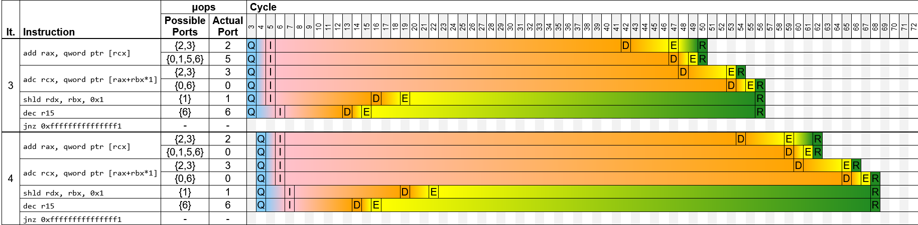
Figure 2. Screenshot of uiCA’s timeline view

4.3. Basic-Block Throughput Predictor

Based on the model described in the previous paragraphs, we have implemented uiCA, a tool that simulates the execution of basic blocks on Intel Core microarchitectures. The tools provides throughput predictions, as well as further insights into how the code is executed, which may be useful for performance engineers. Specifically, it can generate a table that contains the actual port usage for each instruction, and it can output a timeline that shows what happens in each cycle; an excerpt from such a timeline is shown in Figure 2.

Throughput predictions for a basic block are obtained as follows. The tool simulates the repeated execution of the basic block for at least 500 cycles and until at least 10 iterations have been completed. Let $n$ be the number of completed iterations. Let $t$ be the cycle in which the last instruction of the $n$-th iteration was retired, and $t^{\prime}$ be the cycle in which the last instruction of the $\frac{n}{2}$-th iteration was retired. The tool then predicts $\frac{2\cdot(t-t^{\prime})}{n}$ as the throughput. This approach is similar to an approach that was proposed in (Abel20, ) for performing measurements. It is based on the assumption that after $\frac{n}{2}$ iterations, a steady state has been reached.

5. Benchmarks and Measurements

To evaluate and compare our predictor to previous approaches, we need a set of suitable benchmarks. Chen et al. (Chen19, ) proposed the BHive benchmark suite, which is designed specifically to evaluate basic-block throughput predictors on x86 systems. The BHive suite contains more than 300,000 basic blocks that were extracted from applications from different domains, including numerical computation, databases, compilers, machine learning, and cryptography.

In addition to the BHive suite, Chen et al. in the same paper also propose a profiling tool to measure the throughput of such basic blocks using hardware performance counters.

While their benchmark suite and measurement framework are in principle suitable for evaluating the work presented in our paper, we discovered a number of issues with their approach that can lead to incorrect or misleading results. Thus, in this section, we describe how to overcome these issues.

5.1. In-Scope Benchmarks

The goal of the BHive benchmark suite is to consist of basic blocks whose execution conforms to the common modeling assumptions of throughput predictors discussed in Section 3.2.

The benchmark suite was originally generated as follows: Chen et al. (Chen19, ) first extracted a large number of basic blocks from different applications. Then, they filtered out benchmarks that are not in scope because they violate common modeling assumptions. We have identified several additional benchmarks that violate such modeling assumptions, and we have therefore extended Chen et al.’s filtering approach accordingly.

TLB Misses

A common modeling assumption of existing throughput predictors is that all memory accesses lead to cache and TLB hits. Chen et al. only filter out blocks with cache misses. We additionally filter out blocks with TLB misses, as such blocks are out-of-scope for the BHive benchmark suite. This was confirmed by the authors of the BHive suite.

Unbalanced x87 Operations

The BHive suite contains several basic blocks that contain an unbalanced number of push or pop operations to the x87 floating-point stack. Correct programs would not execute such blocks repeatedly in isolation, as this leads to stack underflows or overflows, which result in penalties of hundreds of cycles. It is worth noting that the basic blocks in the BHive benchmark suite are not necessarily executed in loops in the applications from which they were extracted, and thus underflows or overflows would not occur in their original contexts.

A common modeling assumption is that no underflows or overflows would occur. We therefore filtered out the corresponding benchmarks, as they are not in scope for the benchmark suite.

Unsupported Instructions

The TZCNT instruction was introduced with the Haswell microarchitecture. It has the same encoding as the BSF instruction with a REP prefix. This prefix is undefined for the BSF instruction; however, older CPUs do not generate an exception in this case, but simply ignore the prefix.

We removed the TZCNT instruction from the benchmarks for older microarchitectures, as it is not meaningful to evaluate throughput predictions on unsupported instructions.

Benchmarks with Input-Dependent Timing

As discussed in Section 3.2, throughput predictors make assumptions on the inputs that are used for basic blocks that have input-dependent timing. However, the inputs that the BHive profiler uses do, in general, not conform to these assumptions. For example, the BHive profiler initializes all register with the same value, which often leads to memory aliasing. It should be noted that in the context from which the basic blocks were originally extracted, it would rarely be the case that all registers have the same value. Moreover, division instructions that use these values are typically fast, which conflicts with the pessimistic assumptions of most throughput predictors for such cases.

Ideally, one should choose initial values such that the execution conforms to the modeling assumptions. However, developing an approach to do so automatically is beyond the scope of this paper; doing it manually is infeasible due to the large number of benchmarks.

Using measurements with the currently used input values to compare throughput predictors is not very meaningful, as it could give an unfair advantage to the tools that were trained on measurements with the same input values. It would also give an unfair advantage to our predictor, as we know the input values that the BHive profiler uses, and thus we could optimize our predictions for these inputs.

We therefore filter out benchmarks that use the DIV, SQRT, and CPUID instructions, as well as benchmarks for which it may depend on the inputs whether there are read-after-write dependencies. However, we do not filter out benchmarks that use the same address registers for reading and writing to memory and that do not modify this register, as these benchmarks always have a read-after-write dependency, independently of the initial values in the address registers. Furthermore, for the microarchitectures to which it applies, we also filter out benchmarks for which it depends on the inputs whether there is a bank conflict, or whether stores can be paired.

5.2. Loop-Based Benchmarks

The benchmarks in the BHive suite do not end in branch instructions. The BHive profiler measures their throughput according to the $TP_{U}$ definition (see Section 3.1). In (Chen19, ; mendis19a, ), these measurements are used to compare the predictions of Ithemal (which was trained on benchmarks that were evaluated with the same profiler) to the predictions of IACA, OSACA, and llvm-mca (which are based on the $TP_{L}$ definition). As the predictions of Ithemal are closer to the measurements than the predictions of the other tools, they conclude that Ithemal “outperforms” the other tools. We don’t think this conclusion is valid because the measurements are based on a different definition of throughput than the predictions of the other tools.

In order to enable a more meaningful comparison with previous tools, we have created a variant of the BHive benchmark suite in which the benchmarks end in a branch instruction, so that they are applicable to the $TP_{L}$ definition. In the following, we will call this benchmark suite BHive_L, and the original benchmark suite BHive_U.

We have generated the benchmarks in BHive_L from those in BHive_U as follows. Let $B$ be a benchmark in BHive_U, and let $R_{x}$ be a general-purpose register that is not used by $B$. We then add to BHive_L an extended benchmark of the form

loop: $B$; DEC $R_{x}$; JNZ loop

Here, $R_{x}$ is used as the loop counter. For a small number of benchmarks in BHive_U, we could not find such a register $R_{x}$, as these benchmarks already use all general-purpose registers. We omitted these benchmarks from BHive_L.

Several of the benchmarks in BHive_U are very small; some of them consist of only a single instruction. For such benchmarks, the execution time of the extended benchmark may be dominated by the loop overhead, which limits the throughput to one iteration per cycle in the best case. Therefore, for benchmarks $B$ with fewer than five instructions, we added an additional variant in which $B$ is unrolled until there are at least five instructions (which corresponds to the maximum issue width of the CPUs that we consider) in the body of the loop.

5.3. Performing Accurate Measurements

For a meaningful comparison of measurements to predictions, it is important that the measurements are performed in an accurate way and in a well-defined setting.

Based on our experience, measurements using hardware performance counters can be almost cycle-accurate if some precautions are taken. Unfortunately, the BHive profiler tool does not always achieve this accuracy. Skylake CPUs, for example, can execute at most two instructions of the same kind with memory operands per cycle. Thus, any measurement with a throughput value smaller than 0.5 cycles per iteration for benchmarks with memory instructions is obviously not accurate. The published measurements file, which was used for the evaluation in (Chen19, ), contains almost 20,000 such cases. More than 2,200 of them even report a throughput value of less than 0.45 cycles per iteration (i.e., the measurements are more than 10% off from the correct value).

One of the reasons for these inaccuracies is that for small basic blocks, the BHive profiler does not use a large enough number of repetitions to actually reach a steady state in all cases. We use the following approach instead. Let $n$ be the number of instructions in a benchmark, and let $r\mathrel{\mathop{\mathchar 58\relax}}=\left\lceil\frac{500}{n}\right\rceil$. For BHive_U, we determine the throughput as the difference between the measured execution times for $r$ and $2\cdot r$ many repetitions, divided by $r$. This leads to a significantly higher repetition count compared to the original BHive profiler for most benchmarks, but it is still small enough so that the code fits in the instruction cache. For BHive_L, we use the difference between $10,000$ and $20,000$ iterations, divided by $10,000$. We perform all measurements with all but one core disabled to prevent disturbances from other processes, and we repeat all throughput measurements 100 times. We then remove the top and bottom 20% of the measured values, which might be outliers due to, e.g., interrupts. Similar to Chen et al., we filter out benchmarks for which the measurements were not stable. Specifically, we filter out benchmarks if the minimum and the maximum of the remaining throughput values differs by more than 0.02 cycles. Otherwise, we use the median of the measurements as the throughput.

Another reason for the inaccuracies is that the BHive profiler executes multiple branch instructions on the critical path (i.e., while performance counting is active). This makes the execution time dependent on the state of the branch predictor, which, in general, leads to unpredictable measurements. Furthermore, the CPUID instruction is used for serialization, which is relatively expensive and has an input-dependent throughput. We instead use the LFENCE instruction for serialization, as recommended in recent work (McCalpin18, ; Abel20, ), and we removed all branches from the critical path (except, of course, for branches that the benchmarks themselves contain).

The measured throughput can also depend on the initial state of the microarchitecture. For a meaningful comparison of measurements to predictions of previous tools, it is important to perform the measurements under conditions that do not contradict assumptions made by these tools. Specifically, we perform all benchmark runs under the following initial conditions. We make sure that all move elimination resources are available by overwriting all registers, we drain all front-end buffers by executing a long enough sequence of 15-byte NOP instructions, and we align the first instruction of the benchmark to a 64-byte cache line.

6. Experimental Evaluation

6.1. Comparison with Other Tools

In this section we compare our tool, uiCA, with several previous tools on all major Intel Core microarchitecture generations that were released in the last ten years, from Sandy Bridge (released in 2011) to Rocket Lake (released in 2021).

We use IACA (iacaGuide, ) in versions 2.3 and 3.0; version 3.0 does not support the older microarchitectures, and we noticed that IACA 2.3 tends to provide more accurate predictions. For llvm-mca, we use version 10.0.0; for the microarchitectures that are supported by DiffTune, we additionally also evaluate llvm-mca in version 8.0.1, as DiffTune is based on this version. We use DiffTune (Renda20, ) at commit 9992f69 with the models from the paper, which are provided at. We use Ithemal at commit 47a5734 with the retrained models from the BHive paper. For CQA, we use version 2.13.2. We use OSACA at commit 63563ec; we do not use the latest released version of OSACA, as we found several bugs in this version that we reported and that were since fixed by the authors in the version we use. In cases in which a tool crashes or does not return a result within a timeout of one hour, we consider the throughput prediction to be $0$.

To compare the different tools, we use the same metrics that were used in  (Chen19, ; Renda20, ):

• The mean absolute percentage error (MAPE) of the predictions relative to the measurements, which is defined as follows. Let $B$ be a set of pairs $(m,p)$ such that $m$ is the measured throughput of a benchmark, and $p$ is the predicted throughput. Then

  $$MAPE(B)=\frac{1}{|B|}\cdot\sum_{(m,p)\in B}\frac{|m-p|}{m}$$

• Kendall’s tau coefficient (Kendall38, ), which is a measure for how well the pairwise ordering is preserved. As argued by Chen et al. (Chen19, ), Kendall’s tau coefficient can be more useful than the MAPE for example for compiler optimizations, where the relative ordering of different candidate programs is more important than their absolute execution times.

As a baseline, we use the following two simple analytical throughput prediction models corresponding to the two throughput definitions discussed in Section 3.1. Let $n$ be the number of instructions in a specific benchmark, and let $m_{r}$ and $m_{w}$ be the number of memory read and write accesses of the benchmark. Furthermore, let $i$ be the issue width (see Section 4.1.2) of the corresponding microarchitecture, and let $w$ be the number of memory write operations that can be performed per cycle.

For the basic blocks in BHive_U, we use

$$TP_{baseline,U}=max\left(\frac{n}{4},\frac{m_{r}}{2},\frac{m_{w}}{w}\right)$$

as the baseline (this is a generalization to other microarchitectures of the baseline that we discussed in the introduction). This value constitutes a lower bound on the execution time of basic blocks without branch instructions, as at most four instructions can be decoded per cycle, and at most two memory read operations can be performed per cycle.

For the benchmarks in BHive_L, we use

$$TP_{baseline,L}=max\left(1,\frac{n-1}{i},\frac{m_{r}}{2},\frac{m_{w}}{w}\right)$$

as the baseline. We do not include a term for the decoding limit here, as the µops for the benchmarks in BHive_L are often delivered from the DSB or the LSD. Instead, $\frac{n-1}{i}$ corresponds to the issue limit; we use $n-1$ instead of $n$, as the last two instructions of such basic blocks are often macro fused. We do not include a term corresponding to the issue limit for $TP_{baseline,U}$, as $i\geq 4$ for all considered microarchitectures. We use $1$ as an additional lower bound, as the benchmarks in BHive_L cannot run faster than one iteration per cycle due to the read-after-write dependency of the decrement operation. Note that the only microarchitecture-specific variables in these formulas are $i$ and $w$; all other variables only depend on the benchmark and are independent of the microarchitecture.

Table 3 shows the results of our evaluation. For completeness and consistency with the evaluations in (Chen19, ; Renda20, ), we also evaluated the tools that are based on the $TP_{L}$ throughput notion on BHive_U (except for CQA, which can only analyze code that ends in a branch instruction); the corresponding entries are printed in gray. For DiffTune, it is not clear which throughput notion is the more meaningful one: DiffTune is essentially llvm-mca (which is based on $TP_{L}$), but it was trained on measurements obtained according to $TP_{U}$.

In most cases, the accuracy on BHive_L is higher than on BHive_U; the exception here are Ithemal and DiffTune, which were trained on measurements that were obtained by unrolling. This shows that, for a meaningful comparison, it is important that measurements and predictions are based on the same definition of throughput (as discussed in Section 3.1).

Table 2. Microarchitectures used for the evaluation

$\mu$Arch	Abbr.	Released	CPU
Rocket Lake	RKL	2021	Intel Core i9-11900
Tiger Lake	TGL	2020	Intel Core i7-1165G7
Ice Lake	ICL	2019	Intel Core i5-1035G1
Cascade Lake	CLX	2019	Intel Core i9-10980XE
Skylake	SKL	2015	Intel Core i7-6500U
Broadwell	BDW	2015	Intel Core i5-5200U
Haswell	HSW	2013	Intel Xeon E3-1225 v3
Ivy Bridge	IVB	2012	Intel Core i5-3470
Sandy Bridge	SNB	2011	Intel Core i7-2600

Table 3. Comparison of different tools on BHive_U and BHive_L

		BHiveU		BHiveL
$\mu$Arch	Predictor	MAPE	Kendall	MAPE	Kendall
RKL	uiCA	0.49%	0.9835	0.92%	0.9755
	Baseline	15.50%	0.7397	9.26%	0.7808
TGL	uiCA	0.97%	0.9769	0.98%	0.9731
	llvm-mca-10	25.74%	0.7049	13.80%	0.8486
	Baseline	17.49%	0.7245	11.25%	0.7413
ICL	uiCA	1.00%	0.9771	0.77%	0.9759
	OSACA	53.80%	0.3143	21.98%	0.4698
	llvm-mca-10	25.38%	0.7030	13.64%	0.8512
	CQA			6.74%	0.8835
	Baseline	17.54%	0.7230	10.84%	0.7510
CLX	uiCA	0.45%	0.9713	0.65%	0.9825
	llvm-mca-10	23.17%	0.7211	13.21%	0.8060
	OSACA	20.83%	0.7511	11.61%	0.8068
	Baseline	15.49%	0.7461	10.31%	0.8021
SKL	uiCA	0.45%	0.9798	0.38%	0.9895
	Ithemal	8.28%	0.8172	13.66%	0.7582
	IACA 3.0	13.49%	0.7802	14.26%	0.8290
	IACA 2.3	11.85%	0.8071	8.42%	0.8477
	OSACA	14.95%	0.7639	11.25%	0.8045
	llvm-mca-10	15.61%	0.7258	12.01%	0.8015
	llvm-mca-8	15.39%	0.7434	11.98%	0.8021
	DiffTune	24.48%	0.6626	104.88%	0.6426
	CQA			7.44%	0.8847
	Measured (Chen19, )	4.40%	0.9113
	Baseline	17.28%	0.7228	10.03%	0.7999
BDW	uiCA	1.08%	0.9805	0.61%	0.9841
	IACA 3.0	14.69%	0.8012	11.47%	0.8725
	IACA 2.3	13.22%	0.8206	5.84%	0.8928
	OSACA	17.52%	0.7456	9.69%	0.8365
	llvm-mca-10	14.23%	0.7793	16.71%	0.8286
	CQA			5.03%	0.9213
	Baseline	16.97%	0.7572	7.44%	0.8332
HSW	uiCA	0.76%	0.9850	0.59%	0.9842
	Ithemal	7.38%	0.8400	16.19%	0.7700
	IACA 3.0	15.04%	0.8080	12.00%	0.8733
	IACA 2.3	13.13%	0.8291	5.79%	0.8925
	OSACA	17.84%	0.7463	9.77%	0.8307
	llvm-mca-10	20.29%	0.7835	18.97%	0.8259
	llvm-mca-8	21.08%	0.7784	19.46%	0.8171
	DiffTune	24.80%	0.6997	138.47%	0.6925
	CQA			5.08%	0.9220
	Measured (Chen19, )	2.49%	0.9379
	Baseline	17.30%	0.7604	7.57%	0.8314
IVB	uiCA	1.51%	0.9608	1.12%	0.9495
	Ithemal	7.08%	0.8212	12.43%	0.7785
	IACA 2.3	13.94%	0.7739	11.54%	0.8271
	OSACA	36.23%	0.4884	24.88%	0.5846
	llvm-mca-10	22.79%	0.7656	20.76%	0.8154
	llvm-mca-8	22.93%	0.7622	20.76%	0.8138
	DiffTune	26.21%	0.6470	82.94%	0.7516
	CQA			4.05%	0.9174
	Measured (Chen19, )	3.15%	0.9246
	Baseline	18.81%	0.7243	14.47%	0.7670
SNB	uiCA	1.91%	0.9612	0.99%	0.9649
	IACA 2.3	11.91%	0.8194	9.95%	0.8482
	OSACA	36.85%	0.5311	24.75%	0.5659
	llvm-mca-10	22.67%	0.8069	18.34%	0.8455
	CQA			4.08%	0.9238
	Baseline	20.28%	0.7517	15.56%	0.7577

Our tool, uiCA, provides the most accurate predictions in all cases. In many cases, the MAPE is lower by an order of magnitude or more compared to the best previous tools. For uiCA, Kendall’s tau coefficient is always higher than for the previous tools; in most cases, it is significantly higher.

On the Cascade Lake, Skylake, Broadwell, and Haswell microarchitectures, the accuracy of OSACA is similar to several other previous tools. On Ice Lake, Ivy Bridge, and Sandy Bridge, however, the accuracy is significantly below the baseline. A possible explanation for this is that for these microarchitectures, there is a relatively large number of instructions that are currently not supported by OSACA; in such cases, OSACA simply ignores these instructions.

Table 4. Influence of the simulation of different microarchitectural components on the prediction accuracy

		BHiveU		BHiveL
$\mu$Arch	Predictor	MAPE	Kendall	MAPE	Kendall
CLX (all benchmarks)	uiCA	0.45%	0.9713	0.65%	0.9825
	uiCA with simple front end	8.57%	0.8602	6.23%	0.9048
	uiCA with simple port assignment	2.37%	0.9280	12.20%	0.8613
	uiCA without micro fusion	8.77%	0.8683	3.31%	0.9545
	uiCA without macro fusion	0.48%	0.9699	8.84%	0.8863
	uiCA without LSD unrolling	0.45%	0.9713	6.72%	0.9246
	Baseline	15.49%	0.7461	10.31%	0.8021
CLX (benchmarks with moves)	uiCA	0.44%	0.9801	0.45%	0.9836
	uiCA without move elimination	1.71%	0.9656	1.67%	0.9616
	uiCA with full move elimination	0.52%	0.9794	0.47%	0.9846
	Baseline	12.99%	0.8352	9.77%	0.8636

Ithemal cannot analyze code that ends in a branch instruction; for the evaluation of Ithemal on BHive_L, we therefore removed the branch instruction, but we kept the instruction that decrements the loop counter in each iteration. On BHive_U, Ithemal provides the best predictions among the previous tools; however, the predictions of uiCA are significantly better. On BHive_L, several other previous tools provide better predictions than Ithemal; in two cases the MAPE is even below the baseline. It is likely that retraining Ithemal on measurements obtained with the methodology described in Section 5 would improve its accuracy on BHive_L. However, we were unable to do so, as the training set is not publicly available.

Unlike in the evaluation in (Renda20, ), DiffTune does not perform better than llvm-mca on our set of benchmarks. Moreover, DiffTune’s accuracy is below the baseline on all supported microarchitectures.

The rows “Measured (Chen19, )” in Table 3 show the difference of the original timing measurements from (Chen19, ) relative to our improved measurements (see Section 5.3). The MAPE of these measurements compared to our measurements is up to $4.4\%$. This shows that the measurement methodology can have an important influence on the results. Moreover, the high level of agreement of our timing measurements with the predictions of our simulator, combined with the fact that our simulator is, unlike the recent machine learning-based approaches, not based on end-to-end timing measurements, gives us confidence that our measurement methodology is more accurate than the previous approach.

Execution Time

For the benchmarks in BHive_U on Skylake, uiCA (which is implemented in Python) requires on average per benchmark around 105 ms, OSACA 1300 ms, IACA 10 ms, llvm-mca 36 ms. For Ithemal it depends: end-to-end it takes around 580 ms; in interactive mode, each additional benchmark requires around 8 ms.

6.2. Influence of Different Components on Prediction Accuracy

We now evaluate how important different components of the model proposed in Section 4 are for obtaining accurate throughput predictions. In Table 4, we compare different variants of our tool in which parts of the model were replaced by simpler implementations. We use the Cascade Lake microarchitecture, as on this microarchitecture, both the LSD and move elimination are enabled.

6.2.1. Simple Front End

In the first variant, we replace our front-end model with one that is unbounded and can always deliver the maximum number of µops to the renamer. This is similar to the models used by many previous tools. For BHive_U, this leads to a large increase in the average error. For BHive_L, the increase is smaller, which is expected, since for these benchmarks, the µops are often delivered from the LSD or the DSB, which have a higher bandwidth than the decoders; however, the error is still almost an order of magnitude higher than with our detailed model.

6.2.2. Simple Port Assignment

For the second variant, we replace the port assignment algorithm that we reverse engineered (see Section 4.1.2) with one that randomly selects (with uniform probability) a port from among the ports that a µop can use. This is similar to the approach described in (Laukemann18, ). For BHive_U, this leads to an error that is almost five times as high, and for BHive_L, to an error that is more than 17 times as high. A main reason for the higher error in the second case is probably that taken branch instructions can only use port 6; with the random port algorithm there is more competition for port 6 from µops which can also use other ports, and which would more frequently be scheduled on one of these other ports by the actual hardware.

6.2.3. No Micro Fusion

For the third variant, we assume that µops from the same instruction cannot be micro fused by the decoders. For BHive_L, this leads to an error that is about five times as high. For BHive_U, the error is almost 18 times as high; the main reason for this is likely that all instructions that are normally decoded to one micro-fused µop now require the complex decoder.

6.2.4. No Macro Fusion

In the fourth variant, we assume that instructions cannot be macro fused. For BHive_U, this makes no difference, as these benchmarks contain no branch instructions. For BHive_L, on the other hand, the error increases by more than an order of magnitude.

6.2.5. No LSD Unrolling

In the next variant, the LSD does not perform unrolling. Again, this leads to no difference for BHive_U. For BHive_L, the error is almost an order of magnitude higher.

6.2.6. Move Elimination

Finally, we evaluate the influence of the move elimination approach that we reverse engineered in Section 4.1.4. For this, we consider only benchmarks that actually contain move instructions, which is the case for more than one third of the benchmarks. We consider two variants. In the first variant, no move instructions are eliminated. This leads to an average error that is more than three times as high. In the second variant, all eligible move instructions are eliminated. For BHive_U, this leads to an error that is about 15% higher, and for BHive_L to an error that is about 6% higher.

7. Conclusions and Future Work

Based on a new parametric pipeline model, we have developed an open-source simulator to predict the throughput of basic blocks that is significantly more accurate than the state of the art. Our experimental evaluation demonstrates that modeling microarchitectural details considered to be rather insignificant in previous work, is in fact crucial for accurate predictions.

Unlike recently proposed machine learning-based techniques, our approach is not based only on end-to-end measurements, but on focused reverse engineering of individual components, which gives a higher confidence that our model is not overfitting to measurement errors. Training and evaluating predictors on measurements obtained with the same, potentially biased, measurement methodology may result in misleading conclusions, as our results show.

While in this work, we focused on predicting the performance of basic blocks, there is nothing that fundamentally limits our model to basic blocks. In fact, combining our model with a branch prediction model to support predictions for instruction sequences involving potentially multiple branches would be relatively straightforward. Similarly, it would be possible to combine it with, e.g., a memory hierarchy simulator to enable predictions that go beyond the typical capabilities of basic-block throughput predictors. Furthermore, it is conceivable to integrate our model into more comprehensive tools, like full-system simulators, or tools that combine static and dynamic analyses.

8. Artifacts

The source code of uiCA, our improved benchmark suite, and the scripts to generate our tables and heatmaps are available on GitHub. A snapshot of the contents of these repositories at the time of writing is also available on Zenodo (zenodo, ).

Additionally, we provide an interactive online version of our tool at uica.uops.info.

Appendix A Heatmaps for Ice Lake

Figure 3. Heatmaps for BHive_U for basic blocks with a measured throughput of less than 10 cycles/iteration on Ice Lake

Figure 4. Heatmaps for BHive_L for basic blocks with a measured throughput of less than 10 cycles/iteration on Ice Lake

Appendix B Heatmaps for Skylake

Figure 5. Heatmaps for BHive_U for basic blocks with a measured throughput of less than 10 cycles/iteration on Skylake

Figure 6. Heatmaps for BHive_L for basic blocks with a measured throughput of less than 10 cycles/iteration on Skylake

Appendix C Heatmaps for Haswell

Figure 7. Heatmaps for BHive_U for basic blocks with a measured throughput of less than 10 cycles/iteration on Haswell

Figure 8. Heatmaps for BHive_L for basic blocks with a measured throughput of less than 10 cycles/iteration on Haswell

Appendix D Heatmaps for Ivy Bridge

Figure 9. Heatmaps for BHive_U for basic blocks with a measured throughput of less than 10 cycles/iteration on Ivy Bridge

Figure 10. Heatmaps for BHive_L for basic blocks with a measured throughput of less than 10 cycles/iteration on Ivy Bridge