A Unified Efficient Pyramid Transformer for Semantic Segmentation

Abstract

Semantic segmentation is a challenging problem due to difficulties in modeling context in complex scenes and class confusions along boundaries. Most literature either focuses on context modeling or boundary refinement, which is less generalizable in open-world scenarios. In this work, we advocate a unified framework (UN-EPT) to segment objects by considering both context information and boundary artifacts. We first adapt a sparse sampling strategy to incorporate the transformer-based attention mechanism for efficient context modeling. In addition, a separate spatial branch is introduced to capture image details for boundary refinement. The whole model can be trained in an end-to-end manner. We demonstrate promising performance on three popular benchmarks for semantic segmentation with low memory footprint. Code will be released soon.

1 Introduction

Semantic segmentation is the task of dense per-pixel predictions of semantic labels. Starting from Fully Convolutional Network (FCN) [41], there has been significant progress in model development [70, 12, 34, 21, 62, 77]. However, different datasets are in favour of distinctive methods. Taking Fig. 1 as an example, datasets like ADE20K [42, 73] with a larger number of classes often encounter the problem of confusion among similar object classes, and thus require context modeling and global reasoning [56]. On the contrary, datasets like Cityscapes [16] with a less number of classes but high image resolution often suffer from boundary ambiguity, demanding careful handling in object boundaries [64, 76, 33]. Hence, this leads to two separate lines of work in this area, i.e., context modeling [63, 65, 71, 21, 26, 67, 56] and exploiting boundary information [4, 8, 45, 46]. It is thus desirable to have a single method that can jointly optimize them. In this work, we introduce such a unified framework with a two-branch design: context branch and spatial branch.

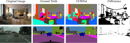
Figure 1: Comparisons of the predictions from OCRNet and the ground truth, and visualizations of their differences. The sample from ADE20K (top) suffers mainly from class confusion, while most errors from Cityscapes (bottom) are along the boundary.

Motivated by the strong capability in capturing long-range contextual dependencies, we extend transformers  [48] to model the per-pixel classification task as a set prediction problem. That is, translating a sequence of RGB pixels into a sequence of object class labels, representing the segmentation mask. Despite reasonable and promising, it is nontrivial to directly apply transformers to such a task. Particularly, as a dense prediction task, semantic segmentation requires: (1) large resolution input image, and (2) the ability of reasoning both local details and the global scene. However, flattening the raw RGB image or even a smaller feature map will result in a much longer sequence than the ordinary linguistic sentence. Fitting such a long sequence for transformer demands prohibitive GPU memory footprint [72]. Furthermore, in order to capture local image details, we need to provide input-adaptive context queries to the transformer decoder.

To address the first issue, we introduce an efficient transformer-based module for semantic segmentation. Specifically, to reduce the memory footprint, we adapt a sparse sampling strategy [75] to enforce each element in a sequence only attending to a small set of elements. The intuition is that only informative surrounding pixels are needed to classify a specific pixel. With this memory-efficient attention module, we can also bring pyramid feature maps from different stages of the backbone to enrich multi-scale information. We term this structure as Efficient Pyramid Transformer (EPT). To address the second issue, we introduce a lightweight spatial branch to capture local image details. Specifically, our spatial branch consists of a three-layer backbone and two heads. We use features from the backbone as context queries to enforce the decoder input adaptive. The two heads are optimized to localize the boundary pixels and eventually used to refine our initial segmentation results from the context branch.

At this point, we present UN-EPT, a UNified Efficient Pyramid Transformer network, to improve both context modeling and boundary handling for semantic segmentation. With UN-EPT, we outperform previous literature with the same backbone (i.e., ResNet50) on ADE20K by a large margin. When combined with a stronger backbone DeiT [47], our method can achieve an mIoU of $50.5$. Notably, our model requires neither pretraining on large-scale dataset (e.g., ImageNet22K), nor the huge memory cost (e.g., our best model only consumes 8.5G memory during training). This clearly demonstrates the effectiveness of our approach. Our contributions can be summarized as:

• We adapt an attention module, termed efficient pyramid transformer, to fully exploit context modeling for semantic segmentation.

• We introduce a spatial branch to provide input-adaptive information and refine object boundaries for final segmentation mask prediction.

• We present a unified framework for both context modeling and boundary handling, which achieves promising results on three benchmark datasets: ADE20K, Cityscapes and PASCAL-Context.

2 Related work

Context modeling Starting from the seminal work of FCN [41], there has been significant progress in models for semantic segmentation. In order to explore context dependencies for improved scene understanding, recent works have focused on exploiting object context by pyramid pooling [70, 10, 11, 12, 53], global pooling [65, 57, 58, 38] and attention mechanism [66]. In terms of the attention mechanism, earlier works [65, 57] adopt channel attention similar to SENet [25] to reweight feature maps as well as learning spatial attention [63, 71, 67, 56]. Most of them directly learn the attention on top of the last convolutional features for context modeling due to GPU memory constraints. In this paper, we exploit a sparse sampling strategy to alleviate the computational cost of attention so that we can fit a long sequence into a transformer. [68, 55] are two closely related works, also introducing efficient sampling method for segmentation. However, both of them still conduct the sampling in a single scale layer while we adopt sampling across multiple pyramid layers for effective context modeling.

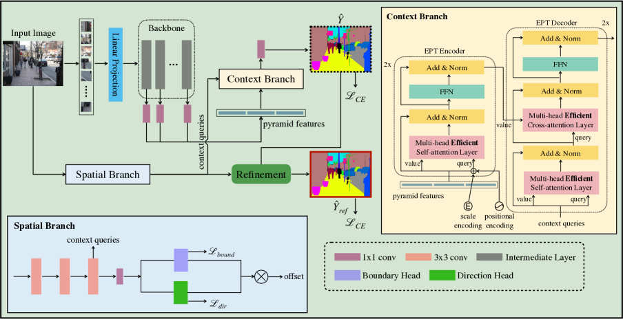
Figure 2: UN-EPT architecture learned in an end-to-end manner. Different backbones can be utilized to extract pyramid visual features (e.g., ResNet, transformer). We show DeiT here for illustration. Image features are flattened into a long sequence and fed into the context branch to obtain the initial segmentation result $\hat{Y}$. The spatial branch extracts features for dynamic context queries and the boundary information to refine $\hat{Y}$. The final refined segmentation output is $\hat{Y}_{ref}$.

Boundary handling Previous works focused on either localizing semantic boundaries [39, 60, 61, 1] or refining boundary segmentation results [4, 46, 19, 45]. They are often designed for images with high resolution, while less useful for modeling contexts, which are prone to error with numerous classes existing. Extensive studies [32, 22, 31, 64] have proposed refinement mechanism to obtain fine segmentation maps from coarse ones, but most of them depend on particular segmentation models. [64] proposes a model-agnostic segmentation refinement mechanism that can be applied to any approaches. However, it still needs re-training and remains a post-processing method. Inspired by [64], we propose a dedicated spatial branch to capture more image details, so that we provide dynamic context queries for the decoder input and utilize boundary information for refinement. Importantly, our method is end-to-end trainable, and can handle the case of a large number of object categories and high resolution images, simultaneously.

Transformer Transformer is a powerful model for capturing long-range contextual dependencies, which is firstly introduced in [48] for machine translation. After that, it has been widely adopted and becomes the de-facto standard in natural language processing [18, 43, 44, 5]. Recently, researchers start to apply transformer in computer vision [75, 20, 72, 52, 40, 13, 50]. SETR [72] directly adopts the ViT [20] model for semantic segmentation. The recent PVT [50] proposes a versatile transformer backbone suitable for several vision tasks. However, the vanilla transformer is computationally heavy and memory consuming when the sequence length is long, which is not scalable for semantic segmentation. The con-current works SegFormer [52] and Swin Transformer [40] use MLP decoders and shifted windows to improve the model efficiency. Different from them, we change the computation strategy of self- and cross-attention and our model jointly considers modeling boundary information, which is specifically suitable for segmentation. MaskFormer [13] solves the semantic- and instance-segmentation in a unified manner by introducing mask predictions. Inspired by the rapid progress of efficient transformers [3, 30, 14, 75], we propose a unified efficient pyramid transformer model for semantic segmentation in this work.

3 Method

This section introduces the proposed UN-EPT network as illustrated in Fig. 2. Particularly, we present an efficient transformer for modeling contexts in Sec. 3.1, including an intuitive sparse sampling strategy to compute attention (Sec. 3.1.1). We then apply pyramid features naturally to fully explore long-range spatial contexts (Sec. 3.1.2). Finally, a spatial branch for segmentation is proposed in Sec. 3.2 by using dynamic context queries and boundary refinement.

3.1 Efficient Transformer for modeling contexts

Revisiting Transformer Transformer takes stacks of self-attention layers in both encoder and decoder. Positional encoding and multi-head structure are designed for providing position information and modeling relations in a higher dimension. The standard multi-head attention [48] projects the same input feature sequence into different feature spaces: key, query, value, denoted as $K\in\mathbb{R}^{n\times d_{m}}$, $Q\in\mathbb{R}^{n\times d_{m}}$, $V\in\mathbb{R}^{n\times d_{m}}$, where $n$ represents the sequence length and $d_{m}$ is the feature dimension. The attention weights is computed based on key and query,

$$A_{m}=\textup{softmax}\left(\frac{QW_{m}^{Q}\left(KW_{m}^{K}\right)^{\textup{T}}}{\sqrt{d_{model}}}\right)$$ (1)

where $W_{m}^{Q},W_{m}^{K}\in\mathbb{R}^{d_{m}\times d_{k}}$ and $A_{m}\in\mathbb{R}^{n\times n}$ denotes the attention weights for head $m=\left\{1,2,...,M\right\}$. Then we compute the attention with weights and value, $\textup{Attn}_{m}=A_{m}VW_{m}^{V}$. Here, $W_{m}^{V}\in\mathbb{R}^{d_{m}\times d_{v}}$ and $\textup{Attn}_{m}\in\mathbb{R}^{n\times d_{v}}$ is the attention value of head $m$. Finally, we concatenate the result of each head to obtain multi-head attention: $\textup{MH-Attn}=\left[\textup{Attn}_{1},...,\textup{Attn}_{M}\right]W^{O}$. Here $W^{O}\in\mathbb{R}^{Md_{v}\times d_{m}}$ denotes linear projection and $\left[\cdot\right]$ denotes the concatenation operation. With the help of multi-head self attention, the transformer encodes the input feature sequence by letting them attend to each other, where the output feature captures long-range contexts, motivating us to apply it to dense per-pixel classification task.

3.1.1 Transformer with sparse sampling

To model the pixel-to-pixel correlation, transformer brings huge cost in memory space and computation resource when an input sequence is relatively long. In the case of segmentation, several problems make the transformer inefficient and impractical in real scenarios: (1) Large input size results in a long pixel feature sequence, making it impossible to fit in a general GPU. (2) Attending to all pixels is unwise and may cause confusion. For instance, to segment different instances of the same category, each pixel only needs to attend to the instance region which it belongs to, where features of unrelated instances are redundant.

To tackle above issues, we adapt a sparse sampling strategy in [75] to semantic segmentation. That is, to force each query pixel to attend only a small set of informative pixels for computing attention. Give an input image, we pass it into a backbone network (e.g., ResNet50 [23] or DeiT [47]) for a feature map $I\in\mathbb{R}^{H\times W\times C}$. Then $I$ is passed by a $1\times 1~{}\textup{conv}$ to reduce channel dimension and sent into the transformer. The input is a sequence of flattened pixel features, denoted as $X\in\mathbb{R}^{HW\times d_{model}}$. We map $X$ to query $Q\in\mathbb{R}^{HW\times d_{model}}$ and value $V\in\mathbb{R}^{HW\times d_{model}}$ features with two parameterized matrice, respectively. Different from the standard self-attention, we do not need key features to compute attention weights here. Instead, our attention weights are learned from query features by a projection matrix.

Then, for each query pixel $q\in Q$ with value as $v$, its attention of head $m$ is computed by

$$\textup{Attn}_{mq}=\textup{softmax}\left(\sum_{n=1}^{N}w_{nq}\right)v_{\left\langle c_{q}+\Delta_{n}\right\rangle}$$ (2)

where $N$ is the number of sparse sampling pixels and $c_{q}$ is the coordinates of $q$. $\left\langle\cdot\right\rangle$ and $\Delta_{n}$ denote the interpolation method and sampling offsets. $w_{nq}$ is the attention weights for $q$ and the $n$-th sampled key element. For simplicity, we omit the linear projection matrice in Eq. 1. Then, for each query element in $Q$, it attends to $N$ value features for calculating attention rather than $HW$ features in $V$, reducing the computation complexity from $O(n^{2})$ to $O(kn)$ ($n=HW$).

To further reduce computation cost, the $\Delta_{n}$ and attention weights $w_{nq}$ $(n=1,2,...,N)$ for $N$ value features are mapped directly from $Q$, which can be written as

$$A_{m}=\textup{softmax}\left(QW_{m}^{Q}U_{m}^{wts}\right),$$ (3)

$$\textup{Attn}_{m}=A_{m}\left(VW_{m}^{V}\right)_{\left\langle QW_{m}^{Q}U_{m}^{pos}\right\rangle}$$ (4)

where $U_{m}^{wts}\in\mathbb{R}^{d_{k}\times N}$ projects the query feature into attention weights and $U_{m}^{pos}\in\mathbb{R}^{d_{k}\times 2N}$ denotes relative positions of key-query in $x$-axis and $y$-axis, as illustrated in [74].

In addition, to inform the model with image spatial information, we add sine and cosine positional encodings on the query $Q$. In practice, the transformer encoder uses the stack of multi-head self-attention layers and feed forward layers to encode the input feature map $X$, and obtains $X_{enc}$ of the same size. On the decoder side, we take a feature $C\in\mathbb{R}^{HW\times d_{model}}$ as input, serving as context queries. It firstly performs self-attention as in Eq. 4 and computes cross-attention with the encoder output $X_{enc}$ to produce final results $\hat{Y}$. The whole process can be written as

$$\hat{Y}=\Phi_{dec}\left(\Phi_{enc}\left(X\right),C\right)$$ (5)

where $\hat{Y}\in\mathbb{R}^{HW\times d_{model}}$ is then up-sampled and computed cross entropy loss with the ground truth. The computation manner of cross attention is the same with self-attention, where the output of decoder self-attention serves as query and $X_{enc}$ is the value feature.

3.1.2 Efficient pyramid transformer

Due to the memory constraint, seldom approaches use multi-scale information for segmentation problem. Here, our model allows us to incorporate pyramid features naturally. As shown in Fig. 2, $1\times 1$ convolutional layers are adopted separately to obtain pyramid feature maps of the same channel size from the backbone, denoted as $\left\{X^{l}\right\}_{l=1}^{L}$, where $X^{l}\in\mathbb{R}^{H_{l}W_{l}\times C}$. To feed into the transformer encoder, they are concatenated in a long sequence $X_{ms}\in\mathbb{R}^{L_{ms}\times d_{model}}$. Similarly, we use linear projections to map $X_{ms}$ to query $Q$ and value $V$ features, respectively. We add positional encoding and scale encoding on $Q$, providing model with more spatial information, as shown in the context branch of Fig. 2. The scale encoding is a learnt embedding of size $L\times d_{model}$. For each query pixel $q$, similar with Eq. 2, it attends to a set of pixels on the feature map of each scale, where the attention is computed as

$$\textup{Attn}_{mq}=\textup{softmax}\left(\sum_{l=1}^{L}\sum_{n=1}^{N}w_{lnq}\right)v_{\left\langle c_{q}+\Delta_{ln}\right\rangle}$$ (6)

where $w_{lnq}$ denotes the attention weight of $q$ and $n$-th sampled key element on the scale $l$. $\Delta_{ln}$ denotes sampling offsets of pixels from each feature scale. Thus, $q$ attends to $N\times L$ pixels, still much less than attending to all $HW$ pixel features. In practice, we set $U_{m}^{wts}\in\mathbb{R}^{d_{k}\times NL}$ and $U_{m}^{pos}\in\mathbb{R}^{d_{k}\times 2NL}$ in Eq. 3 and 4.

The encoder output $X_{enc}\in\mathbb{R}^{L_{ms}\times d_{model}}$ is then fed into the decoder to compute cross attention. We keep the decoder input (context queries) of size $H_{L}W_{L}\times d_{model}$ to recover the image resolution through computing cross attention with $X_{enc}$. Here, context queries reason from pyramid features and select informative pixels to generate predictions. The output is up-sampled to compute the loss. With pyramid features, we are able to model stronger spatial contexts.

3.2 Dynamic learnable spatial branch

Compared to image classification and object detection, one major difference of using transformer for semantic segmentation is that we need high frequency image details for the dense prediction. However, when the transformer is applied to vision tasks, like DETR [7], input queries for decoders are fixed embeddings for all images, which are designed to learn the global information for the dataset. This specific information may not be suitable for segmentation problem. To alleviate it, we introduce a spatial branch to adapt to various input images. We further leverage the spatial branch to capture the boundary information, since its outputs are in relatively high resolutions and maintain more image details. We adopt two additional heads to predict boundary pixels (boundary head) and the corresponding interior pixel for each boundary pixel (direction head). The offset generated from these two predictions is used to refine the segmentation result from the context branch.

Context queries The decoder input serves as context queries, which has different design choices. The naive choice [7] is using a random initialized embedding. However, that embedding will be the same for all input images at inference time, which cannot provide sufficient contextual information. Thus, we introduce dynamic contexts as the decoder input to flourish the self- and cross-attention. As shown in the spatial branch of Fig. 2, our spatial branch contains three $3\times 3$ convolutional layers, followed by batch normalization and ReLU, to extract representations from input images. This branch produces output feature map that is 1/8 of the original image, encoding rich and detailed spatial information due to the large spatial size. Empirically, we choose the intermediate feature from spatial branch to be context queries.

Boundary refinement Inspired by the success of SegFix [64], we adopt a boundary head and a direction head to extract boundary information from the output feature map of the backbone. Similarly, the boundary head contains $1\times 1~{}\textup{Conv}\rightarrow\textup{BN}\rightarrow\textup{ReLU}$ with 256 output channels. A linear classifier ($1\times 1~{}\textup{Conv}$) and up-sampling are further applied to generate the final boundary map of size $H\times W\times 1$. The boundary loss is the binary cross-entropy loss, denoted as $\mathcal{L}_{bound}$. For the direction head, we directly discrete directions by dividing the entire direction range to $m$ partitions as the same as the ground truth ($m=8$ by default). The direction head contains $1\times 1~{}\textup{Conv}\rightarrow\textup{BN}\rightarrow\textup{ReLU}$ with 256 output channels. A linear classifier  ($1\times 1~{}\textup{Conv}$) and up-sampling are further applied to generate the final direction map of size $H\times W\times m$. The direction map is multiplied by the boundary map to ensure direction loss is only applied on boundary pixels. The cross-entropy loss is used to supervise the discrete directions, denoted as direction loss $\mathcal{L}_{dir}$. For the refinement process, we convert the predicted direction map to the offset map of size $H\times W\times 2$. The mapping scheme follows [64]. Then, we generate the refined label map through shifting the coarse label map with the grid-sample scheme [27]. There are multiple mechanisms to generate ground truth for the boundary maps and the direction maps. In this work, we mainly use the conventional distance transform [28], similar with [64]. The final loss function is

$$\mathcal{L}=\lambda_{1}\mathcal{L}_{CE}(Y,\hat{Y})+\lambda_{2}\mathcal{L}_{CE}(Y,\hat{Y}_{ref})+\lambda_{3}\mathcal{L}_{bound}+\lambda_{4}\mathcal{L}_{dir}$$ (7)

where $\hat{Y}_{ref}$ is the refined segmentation result. In practice, we set $\lambda_{1}=1$, $\lambda_{2}=1.5$, $\lambda_{3}=3$, $\lambda_{4}=0.7$.

4 Experiments

We first introduce experimental settings including datasets in Sec. 4.1 and implementation details in Sec. 4.2. We then analyze our results on three benchmark datasets, by comparing with state-of-the-art methods in Sec. 4.3. Following that, we conduct several ablation studies on ADE20K in Sec. 4.4.

4.1 Datasets

Our proposed UN-EPT is evaluated on three standard segmentation benchmarks, i.e., ADE20K dataset [73], PASCAL-Context dataset [42] and Cityscapes dataset [16].

ADE20K dataset [73] is a recent scene parsing benchmark containing dense labels of 150 object category labels. It is challenging due to its large number of classes and existence of multiple small objects in complex scenes. This dataset includes 20K/2K/3K images for training, validation and test. We train our model on the training set and evaluate on the validation set.

PASCAL-Context dataset [42] provides dense annotations for the whole scene in PASCAL VOC 2010, which contains 4998/5105/9637 images for training, validation and test. Following previous works [65, 78], we use 60 class labels (59 object categories plus background) for training and testing. Our results are reported on the validation set.

Cityscapes dataset [16] is a large urban street dataset particularly created for scene parsing, including 19 object categories. It contains 2975/500 fine annotated images for training and validation. Additionally, it has 20000 coarsely annotated training images, but we only use fine annotated training images and report results on the validation set. And there are 1,525 images for testing. We only use fine annotated training images in our setting and we report the results on test set which contains 1525 images.

Method	Reference	Backbone	mIoU	pixAcc
PSPNet [70]	CVPR2017	ResNet50	41.7	80.0
PSANet [71]	ECCV2018	ResNet50	42.9	80.9
UperNet [51]	ECCV2018	ResNet50	41.2	79.9
EncNet [65]	CVPR2018	ResNet50	41.1	79.7
CFNet [67]	CVPR2019	ResNet50	42.9	-
CPNet [56]	CVPR2020	ResNet50	44.5	81.4
Ours	-	ResNet-50	46.1	81.7
RefineNet [36]	CVPR2017	ResNet101	40.2	-
PSPNet [70]	CVPR2017	ResNet101	43.3	81.4
SAC [69]	ICCV2017	ResNet101	44.3	81.9
UperNet [51]	ECCV2018	ResNet101	42.7	81.0
DSSPN [35]	CVPR2018	ResNet101	43.7	81.1
PSANet [71]	ECCV2018	ResNet101	43.8	81.5
EncNet [65]	CVPR2018	ResNet101	44.7	81.7
ANL [78]	ICCV2019	ResNet101	45.2	-
CCNet [26]	ICCV2019	ResNet101	45.2	-
CFNet [67]	CVPR2019	ResNet101	44.9	-
CPNet [56]	CVPR2020	ResNet101	46.3	81.9
OCRNet [62]	ECCV2020	ResNet101	45.3	-
Efficient FCN [37]	ECCV2020	ResNet101	45.3	-
ResNeSt [66]	arXiv2020	ResNeSt200	48.4	-
SETR [72]	CVPR2021	T-large	50.2	83.5
Ours	-	DeiT	50.5	83.6

Table 1: Quantitative evaluations on the ADE20K validation set.

4.2 Implementation details

We implement our experiments with PyTorch [78] and MMSegmentation [15] open source toolbox.

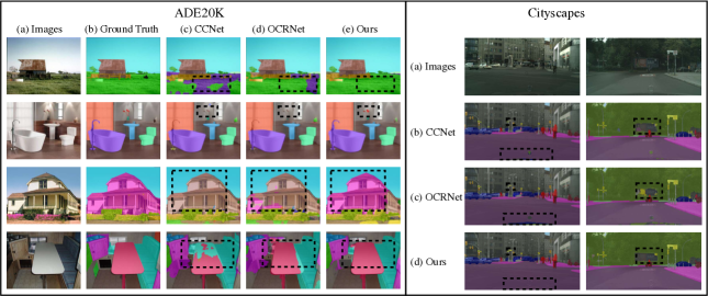
Figure 3: Qualitative results of proposed UN-EPT on three datasets. We compare our method with CCNet [26] and OCRNet [62]. We visualize them with models released from MMSegmentation. On ADE20K and PASCAL-Context, our model deals with contexts and small objects better. And our model handles the boundary artifacts better on Cityscapes. See black dashed boxes for differences, best zoomed in.

Network structure For the ResNet50 [23] backbone, we use ImageNet pre-trained weights as initialization and apply the dilation strategy [9, 59] to obtain 1/8 output size of the input image. The $1\times 1$ convolutional layer is used to reduce the channel dimension of backbone features to $d_{model}=256$. We take intermediate features from stage 3 to 5 in the backbone to obtain pyramid features. For the stronger backbone DeiT [47], we use the base version with a 12-layer encoder. We set the patch size as $16\times 16$ and adapt the positional encoding with bilinear interpolation. For pyramid features, we extract pyramid features from outputs of the 4th, 8th, 12th layer followed by $1\times 1$ convolutional layers. The embedded dimension of the encoder layer is 768, with the head number as 12. We use the model weights from [47] as pretrained weights, which are trained with ImageNet1K. The dimensions of positional encoding and scale encoding are the same with $d_{model}$ and they are added with pyramid features to serve as transformer encoder inputs. For EPT, we use 2 encoders and decoders with head number being $M=8$ and $d_{k}=d_{v}=32$. The hidden dimension of the feed forward layer is 2048. We model the residual inside transformer layers and layer normalization is applied. The dropout strategy is applied after the linear layer in the attention computation and after two linear layers of the feed forward module. For UN-EPT, we empirically set $N=16$ and $L=3$. That is, selecting 16 pixels on the feature map of each scale for computing attention. On the encoder side, we map the query feature (image feature) to offsets for sampling pixels. On the decoder side, we also map the query feature to offsets of sampling features. The output predictions are upsampled 8 times by bilinear interpolation for cross entropy loss. The whole framework is trained in an end-to-end manner.

Evaluation metrics We use standard segmentation evaluation metrics of pixel accuracy (pixAcc) and mean Intersection of Union (mIoU). For the ADE20K dataset, we follow the standard benchmark [73] to ignore background pixels for computing mIoU. For Cityscapes, we report our results by submitting to the test server.

Training For data augmentation, we randomly scale the image with ratio range from 0.5 to 2.0. Random horizontal flipping, photometric distortion and normalization are further adopted to avoid overfitting. Images are then cropped or padded to the same size to feed into the network ($480\times 480$ for ADE20K and PASCAL-Context and $768\times 768$ for Cityscapes). We train 160k iterations for the ADE20K dataset and 80k iterations for the Cityscapes dataset. The base learning rate is 1e-4 except that the base learning rate of backbone layers is 1e-5. The learning rates are dropped at 2/3 iteration with 0.1. We use AdamW optimizer with weight decay being 1e-4, $\beta_{1}=0.9$ and $\beta_{2}=0.999$. We set batch size as 16 for all experiments and synchronized batch normalization is utilized. For all ablation experiments, we run the same training recipe five times and report the average mIoU and pixAcc.

Inference At inference time, following [70, 58, 65, 56], we apply scaling (scale ratio: $\left\{0.5,0.75,1.0,1.25,1.5,1.75\right\}$), flipping and normalization to augment test inputs and obtain the average predictions as final outputs.

Method	Backbone	mIoU
PSPNet [70]	ResNet101	78.5
DeepLabv3 [11] (MS)	ResNet101	79.3
PointRend [29]	ResNet101	78.3
OCRNet [62]	ResNet101	80.6
Multiscale DEQ [2] (MS)	MDEQ	80.3
CCNet [26]	ResNet101	80.2
GCNet [6]	ResNet101	78.1
Axial-DeepLab-XL [49] (MS)	Axial-ResNet-XL	81.1
Axial-DeepLab-L [49] (MS)	Axial-ResNet-L	81.5
SETR [72] (MS)	T-large	82.2
Ours (80k, MS)	ResNet50	79.8
Ours (80k, MS)	DeiT	82.9

Table 2: Quantitative evaluations on the Cityscapes validation set (training iterations: 80k, MS: Multi-scale inference).

Method	Reference	Backbone	mIoU
RefineNet [36]	CVPR2017	ResNet101	73.6
PSPNet [70]	CVPR2017	ResNet101	78.4
SAC [69]	ICCV2017	ResNet101	78.1
BiSeNet [57]	ECCV2018	ResNet101	78.9
PSANet [71]	ECCV2018	ResNet101	80.1
ANL [78]	ICCV2019	ResNet101	81.3
CPNet [56]	CVPR2020	ResNet101	81.3
OCRNet [62]	ECCV2020	ResNet101	81.8
CDGC [24]	ECCV2020	ResNet101	82.0
SETR [72]	CVPR2021	T-large	81.6
Ours	-	ResNet50	80.6
Ours	-	DeiT	82.2

Table 3: Quantitative evaluations on the Cityscapes test set.

4.3 Comparison to state-of-the-art

Results on ADE20K dataset. Here, we show both quantitative and qualitative results on ADE20K dataset. For ADE20K, the complexity is mainly due to large class number and existence of small objects. We first report the results trained with a ResNet50 backbone. From Tab. 1, we achieve $46.1$ in terms of mIoU, $1.6$ higher than previous state-of-the-art CPNet [56] trained with ResNet50. We also want to emphasize that ours with ResNet50 obtain competitive performance compared to previous methods trained with ResNet101. In addition, we can achieve state-of-the-art performance with a stronger backbone network, i.e. DeiT [47]. Compared to recent transformer-based method SETR [72], our DeiT-base model pretrained on ImageNet1K even outperforms its ViT-large model pretrained on ImageNet22K.

Next we show several visualizations in Fig. 3, our method can model contextual information well under the circumstance of complex classes, indicating transformer based attention is applicable to explore spatial correlations. Compared with recent methods CCNet [26] and OCRNet [62], our method can distinguish objects without confusing with other object categories, as in the 1st, 3rd, 4th rows of Fig. 3. Besides, our method is able to segment small objects, producing fine-grained results (the 2nd row in Fig. 3).

Results on Cityscapes dataset. Here, we show both quantitative and qualitative results on Cityscapes dataset. We adopt the best recipe in practice. Tables 2 and 3 show the comparative results on the validation and test set of Cityscapes, respectively. We achieve $82.2$ in terms of mIoU, with a DeiT structure as the backbone. We can see that our model outperforms most of concurrent works. We only train the model with the fine annotated images.

Results on PASCAL-Context dataset. Table 4 shows segmentation results on PASCAL-Context. We achieve $55.2$ in terms of mIoU, outperforming DANet [21] and CPNet [56] in modeling contexts with either attention mechanisms or contextual priors. This indicates our advantage in modeling contextual information through an efficient Transformer-based module. Note that, SETR outperforms us by a small margin, but with a larger network (ViT-large) and better pretraining (ImageNet21K).

Method	Reference	Backbone	mIoU
FCN-8S [41]	CVPR2015	VGG16	37.8
BoxSup [17]	ICCV2015	VGG16	40.5
RefineNet [36]	CVPR2017	ResNet152	47.3
PSPNet [70]	CVPR2017	ResNet101	47.8
EncNet [65]	CVPR2018	ResNet101	51.7
DANet [21]	CVPR2019	ResNet101	52.6
ANL [78]	ICCV2019	ResNet101	52.8
CPNet [56]	CVPR2020	ResNet101	53.9
OCRNet [62]	ECCV2020	ResNet101	54.8
Efficient FCN [37]	ECCV2020	ResNet101	55.3
SETR [72]	CVPR2021	T-large	55.8
Ours	-	ResNet50	49.5
Ours	-	DeiT	55.2

Table 4: Quantitative evaluations on the PASCAL-Context validation set.

Variants	pixAcc	mIoU
baseline	80.3	42.3
+ pyramid features	81.1	45.0
+ spatial path	81.7	46.1
+ stronger backbone	83.6	50.5

Table 5: Evaluation of different components on ADE20K validation set.

Feature scales (L)	Sampling points (N)	pAcc	mIoU
1	4	77.5	37.5
	16	80.3	42.5
	64	80.5	42.9
3	4	80.6	44.1
	16	81.7	46.1
	64	80.4	45.6

Table 6: Ablation studies on different sampling points ($N$) and different feature scales ($L$) on ADE20K dataset with a ResNet50 backbone. Note that, boundary refinement is not applied here.

4.4 Ablation studies

Different components. To examine the effectiveness of different components, we conduct a series of experiments by adding one component at a time, e.g. pyramid features, spatial branch for dynamic context and boundary refinement, a stronger attention backbone. All models are trained on ADE20K training set and evaluated on the validation set. As shown in Tab. 5, utilizing pyramid features can improve the mIoU from 42.3 to 45.0 on ADE20K. By further adopting a spatial branch to produce the decoder input and explore boundary information, the mIoU can improve with a 1.1 margin, indicating the benefits in learning from abundant contexts and boundary information. Besides, we show that a stronger attention model is able to extract useful features for better context modeling, improving the mIoU with a large margin (4.5).

Different number of sampling points. Next, we study the effect of using different number of sampling points. Firstly, we set $N=4,16,64$ for the single scale setting, respectively. As shown in Tab. 6, sampling more points to compute attention improves the mIoU to a certain extent, but the number of 16 is sufficient for boosting the mIoU. For pyramid features, we sample 4, 16, 64 points on feature map of each scale. We find that the number of sampling points does not have a large impact on mIoU performance and sampling 16 points on each single scale feature map consistently produces higher performance. Thus, in practice, we set $N=16$ in experiments. Furthermore, incorporating points from pyramid features is always able to improve the performance, showing the effectiveness of the proposed UN-EPT in learning long-range dependencies.

Method	#Params.	GFLOPs	mIoU
PSANet [71]	73M	239.5	43.8
UperNet [51]	86M	226.2	44.9
EncNet [65]	56M	192.2	44.7
CCNet [26]	69M	244.6	45.2
PointRend [29]	48M	526.5	41.6
DNLNet [54]	70M	244.1	45.9
OCRNet [62]	71M	144.8	44.9
SETR [72]	401M	-	50.2
Ours	94M	99.1	50.5

Table 7: Comparison of the number of model parameters. We report numbers from models trained on ADE20K. Models are obtained from MMSegmentation [15] or re-implemented.

Method	Backbone	Mem Cost	mIoU
Sparse Transformer [14]	ResNet50	18.6G	40.3
Longformer [3]	ResNet50	11.3G	39.4
Reformer [30]	ResNet50	15.5G	38.2
CCNet [26]	ResNet50	9.8G	43.1
ANL [78]	ResNet50	2.0G	42.6
SETR [72]	T-large	30.0G	50.2
Ours	ResNet50	7.0G	46.1
Ours	DeiT	8.5G	50.5

Table 8: Ablation studies on the memory efficiency of UN-EPT. We report results on ADE20K validation set.

Efficient transformer We study the effects of efficient transformers in the NLP area, to compare with the proposed UN-EPT. In particular, we adopt Sparse Transformer [14], Reformer [30] and Longformer [3], respectively. We adopt their transformer structures in our model. Sparse Transformer [14] and Longformer [3] are similar in adopting strided/dilated sliding window to attend to a set of regions instead of full attention, saving memory as well as computation cost. But positions of the attended points are relatively fixed for a particular pixel, which is not suitable for complex scenes generally in the segmentation task. Reformer [30] reduces the complexity by using locality-sensitive hashing and reversible residual layers. However, it cannot remedy the lack of context modeling in our case. Thus, the efficient transformers in NLP area truly reduce the memory cost in our case, but they fail to boost the performance, compared with our UN-EPT, as shown in Tab. 8. Our method takes up even less GPU memory and improves the mIoU metric with a large margin. We also compare our UN-EPT with efficient structures for segmentation, i.e., CCNet [26], ANL [78]. The results in Tab. 8 show that our UN-EPT can continuously show competitive performance. In addition, we highlight our efficiency in adopting Transformer-based attention, compared with the recent work SETR [72]. Our method saves the memory cost to a large extent as well as producing better segmentation results. We also compare the number of model parameters and GFLOPs in Tab. 7. Notably, our UN-EPT has the lowest GFLOPs among all methods, showing its high computational efficiency.

Efficiency of the boundary refinement We verify the effectiveness of the spatial branch for boundary refinement in Fig. 4. Predictions after the refinement module (bottom) often have better boundary estimation than them before the module (top).

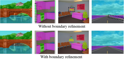
Figure 4: Visualization of segmentation results with/without boundary refinement. Examples are taken from ADE20K validation set.

5 Conclusion

To summarise, we present a unified framework to tackle the problem of semantic segmentation, by both considering context modeling and boundary refinement. We adapt a sparse sampling strategy and use pyramid features to better model contextual information as well as maintaining efficiency. By adding a spatial path, the model captures dynamic contexts as well as fine-grained boundary signals. We hope the proposed UN-EPT method can advocate future work to jointly optimize the contexts and boundary signals for semantic segmentation.

Appendix

Appendix A Pyramid Features

In the experiments, we adopt three feature maps from different stages of the backbone network. These feature maps are concatenated as a long sequence and serve as the encoder input. We use principal component analysis to reduce the dimension of intermediate feature maps and visualize them in Fig. 5. We can see that feature maps from different stages capture image details from different perspectives, providing the transformer encoder with more abundant information.

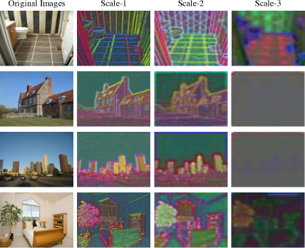
Figure 5: Visualization of pyramid feature maps of UN-EPT trained on ADE20K. We take features from C3-C5 stages of the ResNet50 backbone (i.e., scale-1 to scale-3). Features from the first scale generally capture more low-level details (e.g., boundary statistics), while features from latter layers encode high-level knowledge. Best viewed in color.

Appendix B Backbone Attention

We use a 12-layer DeiT [47] as our backbone network. We visualize the joint learned attention maps of UN-EPT in Fig. 6. It shows that the backbone network can attend to objects of different scales and is able to capture contextual information.

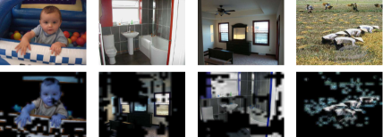
Figure 6: Visualization of attention maps of DeiT trained on ADE20K. We compute the joint attention maps from attention weights of 12 layers, where areas with low attention weights are masked. We can see that the backbone can attend to semantically meaningful regions, beneficial for semantic segmentation. Best viewed in color.

Appendix C Sparse Sampling Visualization

We use a sparse sampling strategy to reduce the computational cost of full self-attention. The model learns to only attend to a set of informative pixel features. We show examples in Fig. 7. From the figure, we can see that a specific query pixel will attend to different sets of points from feature maps of different scales. The distribution of sampled points is able to capture the contextual information of the query pixel.

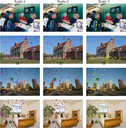
Figure 7: Visualization of sampled points of UN-EPT trained on ADE20K. The green five-pointed star denotes a specific query pixel. We show its sampled points on feature maps of three scales. For each scale in the figure, a specific query pixel attends to $L\times N\times M$ pixel features ($L$: scale number, $N$: #points per scale, $M$: head number). We can see that the query pixel attends to different pixels on features of different scales. Compared with full attention, attending to a set of pixels improves the model efficiency a lot. Best viewed in color.

Appendix D Per-class Analysis on ADE20K

To further analyze the segmentation results and find pros and cons of our method, we choose 20 classes from the total 150 classes in ADE20K, where UN-EPT outperforms state-of-the-art methods, CCNet [26] and OCRNet [62]. Seen from Fig. 8, our proposed method is able to better segment objects with complex contexts, e.g. field, rock, hood, which are always surrounded by other candidate objects. Especially, our method shows competitive results in segmenting small objects, e.g. clock, glass, shower, bag, indicating the benefits gained from pyramid features.

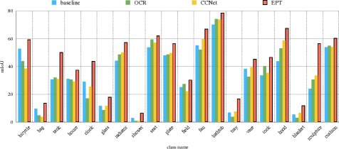
Figure 8: Per-class mIoU results on ADE20K validation set. We choose 20 out of 150 classes for comparison, where UN-EPT outperforms our baseline (single-scale sparse sampled transformer), CCNet [26] and OCRNet [62].

References

- [1] David Acuna, Amlan Kar, and Sanja Fidler. Devil is in the edges: Learning semantic boundaries from noisy annotations. In CVPR, 2019.
- [2] Shaojie Bai, Vladlen Koltun, and J Zico Kolter. Multiscale deep equilibrium models. In NeurIPS, 2020.
- [3] Iz Beltagy, Matthew E Peters, and Arman Cohan. Longformer: The long-document Transformer. arXiv, 2020.
- [4] Gedas Bertasius, Jianbo Shi, and Lorenzo Torresani. Semantic segmentation with boundary neural fields. In CVPR, 2016.
- [5] Tom B Brown, Benjamin Mann, Nick Ryder, Melanie Subbiah, Jared Kaplan, Prafulla Dhariwal, Arvind Neelakantan, Pranav Shyam, Girish Sastry, Amanda Askell, et al. Language models are few-shot learners. arXiv, 2020.
- [6] Yue Cao, Jiarui Xu, Stephen Lin, Fangyun Wei, and Han Hu. Gcnet: Non-local networks meet squeeze-excitation networks and beyond. In ICCV workshops, 2019.
- [7] Nicolas Carion, Francisco Massa, Gabriel Synnaeve, Nicolas Usunier, Alexander Kirillov, and Sergey Zagoruyko. End-to-end object detection with Transformers. arXiv, 2020.
- [8] Liang-Chieh Chen, Jonathan T Barron, George Papandreou, Kevin Murphy, and Alan L Yuille. Semantic image segmentation with task-specific edge detection using cnns and a discriminatively trained domain transform. In CVPR, 2016.
- [9] Liang-Chieh Chen, George Papandreou, Iasonas Kokkinos, Kevin Murphy, and Alan L Yuille. Semantic image segmentation with deep convolutional nets and fully connected CRFs. arXiv preprint, 2014.
- [10] Liang-Chieh Chen, George Papandreou, Iasonas Kokkinos, Kevin Murphy, and Alan L Yuille. DeepLab: Semantic image segmentation with deep convolutional nets, atrous convolution, and fully connected CRFs. TPAMI, 2017.
- [11] Liang-Chieh Chen, George Papandreou, Florian Schroff, and Hartwig Adam. Rethinking atrous convolution for semantic image segmentation. arXiv preprint, 2017.
- [12] Liang-Chieh Chen, Yukun Zhu, George Papandreou, Florian Schroff, and Hartwig Adam. Encoder-decoder with atrous separable convolution for semantic image segmentation. In ECCV, 2018.
- [13] Bowen Cheng, Alexander G Schwing, and Alexander Kirillov. Per-pixel classification is not all you need for semantic segmentation. arXiv, 2021.
- [14] Rewon Child, Scott Gray, Alec Radford, and Ilya Sutskever. Generating long sequences with sparse Transformers. arXiv, 2019.
- [15] MMSegmentation Contributors. MMSegmentation: Openmmlab semantic segmentation toolbox and benchmark. https://github.com/open-mmlab/mmsegmentation, 2020.
- [16] Marius Cordts, Mohamed Omran, Sebastian Ramos, Timo Rehfeld, Markus Enzweiler, Rodrigo Benenson, Uwe Franke, Stefan Roth, and Bernt Schiele. The Cityscapes dataset for semantic urban scene understanding. In CVPR, 2016.
- [17] Jifeng Dai, Kaiming He, and Jian Sun. BoxsUp: Exploiting bounding boxes to supervise convolutional networks for semantic segmentation. In ICCV, 2015.
- [18] Jacob Devlin, Ming-Wei Chang, Kenton Lee, and Kristina Toutanova. BERT: Pre-training of deep bidirectional Transformers for language understanding. arXiv, 2018.
- [19] Henghui Ding, Xudong Jiang, Ai Qun Liu, Nadia Magnenat Thalmann, and Gang Wang. Boundary-aware feature propagation for scene segmentation. In ICCV, 2019.
- [20] Alexey Dosovitskiy, Lucas Beyer, Alexander Kolesnikov, Dirk Weissenborn, Xiaohua Zhai, Thomas Unterthiner, Mostafa Dehghani, Matthias Minderer, Georg Heigold, Sylvain Gelly, et al. An image is worth 16x16 words: Transformers for image recognition at scale. arXiv, 2020.
- [21] Jun Fu, Jing Liu, Haijie Tian, Yong Li, Yongjun Bao, Zhiwei Fang, and Hanqing Lu. Dual attention network for scene segmentation. In CVPR, 2019.
- [22] Spyros Gidaris and Nikos Komodakis. Detect, replace, refine: Deep structured prediction for pixel wise labeling. In CVPR, 2017.
- [23] Kaiming He, Xiangyu Zhang, Shaoqing Ren, and Jian Sun. Deep residual learning for image recognition. In CVPR, 2016.
- [24] Hanzhe Hu, Deyi Ji, Weihao Gan, Shuai Bai, Wei Wu, and Junjie Yan. Class-wise dynamic graph convolution for semantic segmentation. arXiv, 2020.
- [25] Jie Hu, Li Shen, and Gang Sun. Squeeze-and-excitation networks. In CVPR, 2018.
- [26] Zilong Huang, Xinggang Wang, Lichao Huang, Chang Huang, Yunchao Wei, and Wenyu Liu. CCNet: Criss-cross attention for semantic segmentation. In ICCV, 2019.
- [27] Max Jaderberg, Karen Simonyan, Andrew Zisserman, and Koray Kavukcuoglu. Spatial Transformer networks. In NeurIPS, 2015.
- [28] Ron Kimmel, Nahum Kiryati, and Alfred M Bruckstein. Sub-pixel distance maps and weighted distance transforms. J. Math. Imaging Vis., 1996.
- [29] Alexander Kirillov, Yuxin Wu, Kaiming He, and Ross Girshick. PointRend: Image segmentation as rendering. arXiv, 2019.
- [30] Nikita Kitaev, Łukasz Kaiser, and Anselm Levskaya. Reformer: The efficient Transformer. arXiv, 2020.
- [31] Weicheng Kuo, Anelia Angelova, Jitendra Malik, and Tsung-Yi Lin. ShapeMask: Learning to segment novel objects by refining shape priors. In ICCV, 2019.
- [32] Ke Li, Bharath Hariharan, and Jitendra Malik. Iterative instance segmentation. In CVPR, 2016.
- [33] Xiangtai Li, Xia Li, Li Zhang, Cheng Guangliang, Jianping Shi, Zhouchen Lin, Yunhai Tong, and Shaohua Tan. Improving semantic segmentation via decoupled body and edge supervision. In ECCV, 2020.
- [34] Xia Li, Zhisheng Zhong, Jianlong Wu, Yibo Yang, Zhouchen Lin, and Hong Liu. Expectation-maximization attention networks for semantic segmentation. In ICCV, 2019.
- [35] Xiaodan Liang, Hongfei Zhou, and Eric Xing. Dynamic-structured semantic propagation network. In CVPR, 2018.
- [36] Guosheng Lin, Anton Milan, Chunhua Shen, and Ian Reid. RefineNet: Multi-path refinement networks for high-resolution semantic segmentation. In CVPR, 2017.
- [37] Jianbo Liu, Junjun He, Jiawei Zhang, Jimmy S Ren, and Hongsheng Li. EfficientFCN: Holistically-guided decoding for semantic segmentation. In ECCV, 2020.
- [38] Wei Liu, Andrew Rabinovich, and Alexander C. Berg. ParseNet: Looking wider to see better. In ICLR, 2016.
- [39] Yun Liu, Ming-Ming Cheng, Xiaowei Hu, Kai Wang, and Xiang Bai. Richer convolutional features for edge detection. In CVPR, 2017.
- [40] Ze Liu, Yutong Lin, Yue Cao, Han Hu, Yixuan Wei, Zheng Zhang, Stephen Lin, and Baining Guo. Swin transformer: Hierarchical vision transformer using shifted windows. arXiv, 2021.
- [41] Jonathan Long, Evan Shelhamer, and Trevor Darrell. Fully Convolutional Networks for Semantic Segmentation. In CVPR, 2015.
- [42] Roozbeh Mottaghi, Xianjie Chen, Xiaobai Liu, Nam-Gyu Cho, Seong-Whan Lee, Sanja Fidler, Raquel Urtasun, and Alan Yuille. The role of context for object detection and semantic segmentation in the wild. In CVPR, 2014.
- [43] Alec Radford, Karthik Narasimhan, Tim Salimans, and Ilya Sutskever. Improving language understanding by generative pre-training, 2018.
- [44] Alec Radford, Jeffrey Wu, Rewon Child, David Luan, Dario Amodei, and Ilya Sutskever. Language models are unsupervised multitask learners. OpenAI Blog, 2019.
- [45] Tao Ruan, Ting Liu, Zilong Huang, Yunchao Wei, Shikui Wei, and Yao Zhao. Devil in the details: Towards accurate single and multiple human parsing. In AAAI, 2019.
- [46] Towaki Takikawa, David Acuna, Varun Jampani, and Sanja Fidler. Gated-SCNN: Gated shape CNNs for semantic segmentation. In ICCV, 2019.
- [47] Hugo Touvron, Matthieu Cord, Matthijs Douze, Francisco Massa, Alexandre Sablayrolles, and Hervé Jégou. Training data-efficient image Transformers & distillation through attention. arXiv, 2020.
- [48] Ashish Vaswani, Noam Shazeer, Niki Parmar, Jakob Uszkoreit, Llion Jones, Aidan N Gomez, Łukasz Kaiser, and Illia Polosukhin. Attention is all you need. In NeurIPS, 2017.
- [49] Huiyu Wang, Yukun Zhu, Bradley Green, Hartwig Adam, Alan Yuille, and Liang-Chieh Chen. Axial-deeplab: Stand-alone axial-attention for panoptic segmentation. In ECCV, 2020.
- [50] Wenhai Wang, Enze Xie, Xiang Li, Deng-Ping Fan, Kaitao Song, Ding Liang, Tong Lu, Ping Luo, and Ling Shao. Pyramid vision transformer: A versatile backbone for dense prediction without convolutions. arXiv, 2021.
- [51] Tete Xiao, Yingcheng Liu, Bolei Zhou, Yuning Jiang, and Jian Sun. Unified perceptual parsing for scene understanding. In ECCV, 2018.
- [52] Enze Xie, Wenhai Wang, Zhiding Yu, Anima Anandkumar, Jose M Alvarez, and Ping Luo. Segformer: Simple and efficient design for semantic segmentation with transformers. arXiv, 2021.
- [53] Maoke Yang, Kun Yu, Chi Zhang, Zhiwei Li, and Kuiyuan Yang. DenseASPP for semantic segmentation in street scenes. In CVPR, 2018.
- [54] Minghao Yin, Zhuliang Yao, Yue Cao, Xiu Li, Zheng Zhang, Stephen Lin, and Han Hu. Disentangled non-local neural networks. In ECCV, 2020.
- [55] Changqian Yu, Yifan Liu, Changxin Gao, Chunhua Shen, and Nong Sang. Representative graph neural network. In ECCV, 2020.
- [56] Changqian Yu, Jingbo Wang, Changxin Gao, Gang Yu, Chunhua Shen, and Nong Sang. Context prior for scene segmentation. In CVPR, 2020.
- [57] Changqian Yu, Jingbo Wang, Chao Peng, Changxin Gao, Gang Yu, and Nong Sang. BiSeNet: Bilateral segmentation network for real-time semantic segmentation. In ECCV, 2018.
- [58] Changqian Yu, Jingbo Wang, Chao Peng, Changxin Gao, Gang Yu, and Nong Sang. Learning a discriminative feature network for semantic segmentation. In CVPR, 2018.
- [59] Fisher Yu and Vladlen Koltun. Multi-scale context aggregation by dilated convolutions. arXiv, 2015.
- [60] Zhiding Yu, Chen Feng, Ming-Yu Liu, and Srikumar Ramalingam. CaseNet: Deep category-aware semantic edge detection. In CVPR, 2017.
- [61] Zhiding Yu, Weiyang Liu, Yang Zou, Chen Feng, Srikumar Ramalingam, B.V.K. Vijaya Kumar, and Jan Kautz. Simultaneous edge alignment and learning. In ECCV, 2018.
- [62] Yuhui Yuan, Xilin Chen, and Jingdong Wang. Object-contextual representations for semantic segmentation. In ECCV, 2020.
- [63] Yuhui Yuan and Jingdong Wang. OCNet: Object context network for scene parsing. arXiv, 2018.
- [64] Yuhui Yuan, Jingyi Xie, Xilin Chen, and Jingdong Wang. Segfix: Model-agnostic boundary refinement for segmentation. In ECCV. Springer, 2020.
- [65] Hang Zhang, Kristin Dana, Jianping Shi, Zhongyue Zhang, Xiaogang Wang, Ambrish Tyagi, and Amit Agrawal. Context encoding for semantic segmentation. In CVPR, 2018.
- [66] Hang Zhang, Chongruo Wu, Zhongyue Zhang, Yi Zhu, Zhi Zhang, Haibin Lin, Yue Sun, Tong He, Jonas Mueller, R Manmatha, et al. ResNeSt: Split-attention networks. arXiv, 2020.
- [67] Hang Zhang, Han Zhang, Chenguang Wang, and Junyuan Xie. Co-occurrent features in semantic segmentation. In CVPR, 2019.
- [68] Li Zhang, Dan Xu, Anurag Arnab, and Philip HS Torr. Dynamic graph message passing networks. In CVPR, 2020.
- [69] Rui Zhang, Sheng Tang, Yongdong Zhang, Jintao Li, and Shuicheng Yan. Scale-adaptive convolutions for scene parsing. In ICCV, 2017.
- [70] Hengshuang Zhao, Jianping Shi, Xiaojuan Qi, Xiaogang Wang, and Jiaya Jia. Pyramid scene parsing network. In CVPR, 2017.
- [71] Hengshuang Zhao, Yi Zhang, Shu Liu, Jianping Shi, Chen Change Loy, Dahua Lin, and Jiaya Jia. PSANet: Point-wise spatial attention network for scene parsing. In ECCV, 2018.
- [72] Sixiao Zheng, Jiachen Lu, Hengshuang Zhao, Xiatian Zhu, Zekun Luo, Yabiao Wang, Yanwei Fu, Jianfeng Feng, Tao Xiang, Philip HS Torr, et al. Rethinking semantic segmentation from a sequence-to-sequence perspective with transformers. In CVPR, 2021.
- [73] Bolei Zhou, Hang Zhao, Xavier Puig, Sanja Fidler, Adela Barriuso, and Antonio Torralba. Scene parsing through ade20k dataset. In CVPR, 2017.
- [74] Xizhou Zhu, Dazhi Cheng, Zheng Zhang, Stephen Lin, and Jifeng Dai. An empirical study of spatial attention mechanisms in deep networks. In ICCV, 2019.
- [75] Xizhou Zhu, Weijie Su, Lewei Lu, Bin Li, Xiaogang Wang, and Jifeng Dai. Deformable DETR: Deformable Transformers for end-to-end object detection. In ICLR, 2021.
- [76] Yi Zhu, Karan Sapra, Fitsum A Reda, Kevin J Shih, Shawn Newsam, Andrew Tao, and Bryan Catanzaro. Improving semantic segmentation via video propagation and label relaxation. In CVPR, 2019.
- [77] Yi Zhu, Zhongyue Zhang, Chongruo Wu, Zhi Zhang, Tong He, Hang Zhang, R. Manmatha, Mu Li, and Alexander Smola. Improving Semantic Segmentation via Self-Training. arXiv, 2020.
- [78] Zhen Zhu, Mengde Xu, Song Bai, Tengteng Huang, and Xiang Bai. Asymmetric non-local neural networks for semantic segmentation. In ICCV, 2019.