Safest Nearby Neighbor Queries in Road Networks (Full Version)

Abstract

Traditional route planning and $k$ nearest neighbors queries only consider distance or travel time and ignore road safety altogether. However, many travellers prefer to avoid risky or unpleasant road conditions such as roads with high crime rates (e.g., robberies, kidnapping, riots etc.) and bumpy roads. To facilitate safe travel, we introduce a novel query for road networks called the $k$ safest nearby neighbors ($k$SNN) query. Given a query location $v_{l}$, a distance constraint $d_{c}$ and a point of interest $p_{i}$, we define the safest path from $v_{l}$ to $p_{i}$ as the path with the highest path safety score among all the paths from $v_{l}$ to $p_{i}$ with length less than $d_{c}$. The path safety score is computed considering the road safety of each road segment on the path. Given a query location $v_{l}$, a distance constraint $d_{c}$ and a set of POIs $P$, a $k$SNN query returns $k$ POIs with the $k$ highest path safety scores in $P$ along with their respective safest paths from the query location. We develop two novel indexing structures called $Ct$-tree and a safety score based Voronoi diagram (SNVD). We propose two efficient query processing algorithms each exploiting one of the proposed indexes to effectively refine the search space using the properties of the index. Our extensive experimental study on real datasets demonstrates that our solution is on average an order of magnitude faster than the baselines.

1 Introduction

Crime incidents such as kidnapping and robbery on roads are not unusual especially in developing countries stubbert2015crime ; natarajan2016crime ; spicer2016street . Street harassment (e.g., eve teasing, sexual assaults) is a common scenario that mostly women experience on roads news1 ; news2 . A traveler typically prefers to avoid a road segment with high crime or harassment rate. Similarly, during unrest in a country, people prefer to avoid roads with protests or riots. Also, elderly or sick people may prefer to avoid bumpy roads. However, traditional $k$ nearest neighbors ($k$NN) queries that find $k$ closest points of interest (POI) (e.g., a fuel station or a bus stop) fail to consider a traveler’s safety or convenience on roads. In real-world scenarios, a user may prefer visiting a nearby POI instead of their nearest one if the slightly longer path to reach the nearby POI is safer than the shortest path to the nearest POI. In this paper, to allow travelers to avoid different types of inconveniences on roads (e.g., crime incidents, harassment, bumpy roads etc.), we introduce a novel query type, called a $k$ safest nearby neighbors ($k$SNN) query and propose novel solutions for efficient query processing.

We use safety score of a road segment to denote the associated convenience/safety of traveling on it. In this context, a user may want to avoid roads with low safety scores. Intuitively, a path is safer if it requires a smaller distance to be travelled on the least safe roads. Based on this intuition, we develop a measure of the Path Safety Score (PSS) by considering the safety scores and lengths of the road segments included in a path, and use it to find the safest path between two locations. Since in real-world scenarios, a user may not want to travel on paths that are longer than a user-defined distance constraint $d_{c}$, we incorporate $d_{c}$ in the formulation of the $k$SNN query as discussed shortly.

Given a set of POIs $P$ on a road network, a query location $v_{l}$ and a distance constraint $d_{c}$, a $k$SNN query returns $k$ POIs (along with paths from $v_{l}$ to them) with the highest PSSs considering only the paths with distances less than $d_{c}$. Consider Fig. 1 that shows $3$ restaurants ($p_{1}$ to $p_{3}$), a query located at $s$ and the Path Safety Scores (PSS) of some paths from $s$ to the three POIs (we formally define PSS in Section 3). Assume a $1$SNN query (i.e., $k=1$) located at $s$ and $d_{c}=10$km. The restaurants that meet the distance constraint are the candidates for the query answer (i.e., $p_{1}$ and $p_{2}$). The POI $p_{3}$ is not a candidate because the length of the shortest path $P_{4}$ between $s$ and $p_{3}$ is 14, which exceeds $d_{c}$. The safest path between $s$ and $p_{1}$ is $P_{1}$. The PSS of $P_{1}$ is 0.4 and its length is $8$km, which is smaller than $d_{c}=10km$. Though the safest path $P_{3}$ between $s$ and $p_{2}$ has a higher PSS than that of $P_{1}$, we do not consider $P_{3}$ because it is longer than $d_{c}=10km$. The PSS of the safest path $P_{2}$ between $s$ and $p_{2}$ within $d_{c}$ is 0.3. Thus, $1$SNN query (also called SNN query) returns $p_{1}$ along with the path $P_{1}$.

Figure 1: An example $k$SNN query for $k=1$ and $d_{c}=10$.

Finding $k$SNNs in a road network is a computational challenge because the number of POIs in the road network and the number of possible paths between a user’s location and a POI can be huge. The processing overhead of a $k$SNN algorithm depends on the amount of required road network traversal and the number of POIs considered for finding the safest nearby POIs. In this paper, we develop two novel indexing structures called Connected Component Tree ($Ct$-tree) and safety score based network Voronoi diagram (SNVD) to refine the search space and propose two efficient algorithms for finding the safest nearby POIs in road networks. In addition, we exploit incremental network expansion (INE) technique PapadiasZMT03 to evaluate $k$SNN queries.

A $Ct$-tree recursively partitions the road network graph into connected and safer subgraph(s) by recursively removing the roads with the smallest safety scores. Each node of the $Ct$-tree represents a subgraph, and for every subgraph, the $Ct$-tree stores some distance related information. By exploiting $Ct$-tree properties and the stored distance information, we develop pruning techniques that avoid exploring unnecessary paths that cannot be the safest ones to reach a POI and have distances less than the distance constraint. Although a number of indexing structures Guttman84 ; BeckmannKSS90 ; LeeLZT12 ; ZhongLTZG15 ; LiCW19 have been developed, they are developed to reduce the processing overhead for finding nearest neighbors and cannot be applied or trivially extended for efficient processing of $k$SNN queries.

In the past, the Voronoi diagram KolahdouzanS04 has also been widely used for finding nearest neighbors with reduced processing overhead. The traditional Voronoi diagram divides the road network graph into subgrpahs such that each subgraph corresponds to a single POI which is guaranteed to be the nearest POI of every query location in this subgraph. We introduce SNVD that guarantees that, for every query location in a subgraph, its unconstrained safest neighbor (i.e., SNN where the distance constraint is ignored) is its corresponding POI. Note that the unconstrained safest neighbor of a query location is not necessarily its SNN depending on the distance constraint specified by the user. By exploiting the SNVD properties, we develop an algorithm to identify the SNNs, and similar to our $Ct$-tree based approach we improve the performance of our SNVD based algorithm with novel pruning techniques to refine the search space.

Incremental Network Expansion (INE) is among the most efficient nearest POI search techniques that do not rely on any distance-based indexing structure. According to our PSS measure, the PSS of a subpath is greater than or equal to that of the path. This property allows us to adapt the INE based approach for finding $k$SNNs. The INE based approach starts the search from a user’s location, progressively expands the search and continues until the required POIs are identified. Our experiments show that our $Ct$-tree and SNVD based algorithms outperform the INE based approach with a large margin.

The steps of a straightforward solution to evaluate $k$SNNs are as follows: (i) identify candidate POIs which are the POIs with Euclidean distance less than the distance constraint $d_{c}$ from the query location; (ii) compute the safest paths with distance less than $d_{c}$ from the query location to each of the candidate POIs; and (iii) select $k$ POIs with the highest path safety scores. This solution would incur very high processing overhead because it requires multiple searches. All of our algorithms find $k$SNNs with a single search in the road network. We consider this straightforward approach as a baseline in our experiments and compare the performance of our algorithms against it.

To the best of our knowledge, no work has so far addressed the problem of finding $k$SNNs and quantified the PSS measure. Our major contributions are as follows:

• We formulate a measure to quantify the PSS by incorporating road safety scores and individual distances associated with the road safety scores. Our solution can be easily extended for any other PSS measure that satisfy certain properties.

• We develop two novel algorithms for processing $k$SNN queries efficiently using a $Ct$-tree and an SNVD, respectively. In addition, we adapt INE based approach for finding the safest nearby POIs. We propose novel pruning techniques to refine the search space and further improve the performance of our algorithms.

• We conduct an extensive experimental study using real datasets that demonstrates that the two proposed algorithms significantly outperform the baseline and the INE based approach.

The rest of this paper is organized as follows. We discuss related work in Section 2. In Section 3, we formally define the $k$SSN query. In Sections 4, 5 and 6, we discuss our solutions based on INE, Ct-tree and SNVD, respectively. Experimental study is presented in Section 7 followed by conclusions and future work in Section 8.

2 Related Work

2.1 Route Planning

A variety of route planning problems have been studied in the past such as: shortest route computation Dijkstra59 ; ZhongLTZG15 which requires to find the path with the smallest overall cost; multi-criteria route planning NadiD11 ; SalgadoCT18 which aims to return routes considering multiple criteria (e.g., length, safety, scenery etc.); obstacle avoiding path planning shen2020euclidean ; LambertG03 ; leenen2012constraint ; BergO06 ; AnwarH17 which returns the shortest path avoiding a set of obstacles in the space; safe path planning AljubayrinQJZHL17 ; AljubayrinQJZHW15 ; KimCS14 that aims to return paths that are safe and short; alternative route planning li2021comparing ; NadiD11 ; li2020continuously where the goal is to return a set of routes significantly different from each other so that the user has more options to choose from; multi-stop route planning (also called trip planning) HashemHAK13 ; SharifzadehKS08 ; SalgadoCT18 which returns a route that passes through multiple stops/POIs satisfying certain constraints; and route alignment SinghSS19 that requires determining an optimal alignment for a new road to be added in the network such that the cost considering different criteria is minimized. Below, we briefly discuss some of these route planning problems most closely related to our work.

Multi-criteria route planning. Existing techniques FuLL14 ; ShahBLC11 ; NadiD11 ; SalgadoCT18 typically use a scoring function (e.g., weighted sum) to compute a single score of each edge considering multiple criteria. Once the score of each edge has been computed, the existing shortest path algorithms can be used to compute the path with the best score. In contrast, our work cannot trivially use the existing shortest path algorithms due to the nature of the PSS. Also, as noted in GalbrunPT16 , it is non-trivial for a user to define an appropriate scoring function combining the multiple criteria. Thus, some existing works GalbrunPT16 ; josse2015tourismo approach the multi-criteria route planning differently and compute a set of skyline routes which guarantees that the routes returned are not dominated by any other routes. This is significantly different from our work as it returns possibly a large number of routes for an origin-destination pair instead of the safest route.

Obstacle avoiding path planning. Inspired by applications in robotics, video games, and indoor venues cheema2018indoor a large number of existing works shen2020euclidean ; LambertG03 ; leenen2012constraint ; BergO06 ; AnwarH17 ; shen2022fast focus on finding the shortest path that avoids passing through a set of obstacles (e.g., walls) in the space. A recent work aims at finding indoor paths that avoid crowds liu2021towards . Even when obstacles are considered as unsafe regions, these works are different from our work because, in our case, the path may still pass through unsafe edges whereas these works assume that the path cannot cross an obstacle (e.g., a shopper cannot move through the walls).

Safe path planning. There are several existing works that consider safety in path planning. In AljubayrinQJZHL17 ; AljubayrinQJZHW15 ; KimCS14 , the authors divide the space into safe and unsafe zones and minimize the distance travelled through the unsafe zones. However, these works are unable to handle different safety levels of roads and do not consider any distance constraint on the paths. In Section 3, we show that our work is more general and is applicable to a wider range of definitions of safe paths. Some other existing works FuLL14 ; GalbrunPT16 ; ShahBLC11 also consider safety, however, they model the problem as multi-criteria route planning and are significantly different from the problem studied in this paper (as discussed above). The most closely related work to our work is Islam21 which develops an INE-based algorithm to find the safest paths between a source and a destination by considering individual distances associated with different safety scores of a path. We use this as a baseline in our work.

The problem studied in this paper is significantly different from the above-mentioned route planning problems. Unlike route planning problems, our problem does not have a fixed destination, (i.e., each POI is a possible destination) and the goal is to find $k$ POIs with the safest paths. In other words, the problem studied in this work is a POI search problem similar to a $k$ nearest neighbor ($k$NN) query. In our experimental study, we adapt the state-of-the-art safe path planning algorithm Islam21 to compute $k$SNNs and compare against it. Specifically, one approach to find $k$SNNs is to compute the safest path using Islam21 for each POI that has Euclidean distance less than $d_{c}$ from the query location. The application of Islam21 to find $k$SNNs requires multiple independent safest path searches and incurs extremely high processing overhead (as shown in our experimental results). Next, we briefly discuss recent works on $k$NN queries.

2.2 $k$ Nearest neighbor Queries

The problem of finding $k$ nearest neighbors (NNs) has been extensively studied in the literature. Researchers have exploited the incremental network expansion (INE), incremental euclidean restriction (IER), and indexing techniques to solve $k$NN queries. INE PapadiasZMT03 progressively explores the road network paths from the query location in order of their minimum distances until $k$ NNs are identified. IER PapadiasZMT03 uses the Euclidean lower bound property that the road network distance between two points is always greater than or equal to their Euclidean distance to find $k$ NNs in the road network. Different indexing technique dependent $k$NN algorithms like Distance Browsing SametSA08 ; SankaranarayananAS05 , ROAD LeeLZT12 , G-tree ZhongLTZG15 and Voronoi diagram KolahdouzanS04 have been developed to refine the search space and reduce the processing overhead. All of the above algorithms except INE are dependent on the distance related properties and cannot be applied or trivially extended for finding $k$ SNNs. An extensive experimental study has been conducted in abeywickrama2016k to compare existing $k$NN algorithms on road networks.

The straightforward application of a NN algorithm for finding $k$ SNNs is prohibitively expensive as it would require two independent traversals of the road network for finding $k^{\prime}>>k$ nearest neighbors as candidate SNNs, and then computing the safest paths from the query location to each of the candidate SNN, respectively. We extend the INE technique to identify $k$ SNNs with a single search in the road network.

3 Problem Formulation

We model a road network as a weighted graph $G=(V,E)$, where $V$ is a set of vertices and $E$ is a set of edges. A vertex $v_{i}\in V$ represents a road junction in the road network and an edge $e_{ij}\in E$ represents a road between $v_{i}$ to $v_{j}$. Each edge $e_{ij}$ is associated with two values $w_{ij}^{d}$ and $w_{ij}^{ss}$. Here, $w_{ij}^{d}$ is a positive value representing the weight of the edge $e_{ij}$, e.g., length, travel time, fuel cost etc. For simplicity, hereafter, we use length to refer to $w_{ij}^{d}$. $w_{ij}^{ss}$ represents the edge safety score (ESS) of $e_{ij}$ (higher the safer). Computing $w^{ss}_{ij}$ is beyond the scope of this paper and we assume safety scores are given as input (e.g., computed using existing geospatial crime mapping approaches chainey2013gis ). Table 1 summarizes the main notations used the paper.

A path $pt_{ij}$ between two vertices $v_{i}$ and $v_{j}$ is a sequence of vertices such that the path starts at $v_{i}$, ends at $v_{j}$, and an edge exists between every two consecutive vertices in the path. Cost of a path $pt_{ij}$ is the sum of the weights of the edges in the path, e.g., total length, total travel time etc. For simplicity, hereafter, we use distance/length to refer to the cost of a path $pt_{ij}$ and denote it as $dist(pt_{ij})$. Let $d_{c}$ be a user-defined distance constraint. We say that a path $pt_{ij}$ is valid if $dist(pt_{ij})<d_{c}$.

Table 1: A list of notations

Notation	Explanation
$G(V,E)$	The road network graph
$e_{ij}$	An edge connecting vertices $v_{i}$ and $v_{j}$
$w_{ij}^{d}$	Weight (e.g., length, travel time) of $e_{ij}$
$w_{ij}^{ss}$	Edge safety score (ESS) of $e_{ij}$
$s^{max}$	Maximum ESS, i.e., $argmax_{e_{ij}\in E}~{}w_{ij}^{ss}$
$v_{l}$	A query location
$d_{c}$	A user-defined distance constraint
$p_{i}$	A POI located at $v_{i}$
$pt_{ij}$	A path from a vertex $v_{i}$ to a vertex $v_{j}$
$dist(pt)$	Sum of weights of edges in $pt$
$pt_{ij}.d_{s}$	Total weight of edges in $pt_{ij}$ with ESS equal to $s$
$pss(pt)$	Path safety score of $pt$
$pt^{sf}_{ij}$	The safest path between $v_{i}$ and $v_{j}$ that has distance less than $d_{c}$
$pt^{sh}_{ij}$	The shortest path between $v_{i}$ and $v_{j}$

3.1 Path Safety Score (PSS)

Intuitively, we want to define a Path Safety Score (PSS) measure that ensures that a path that requires smaller distance to be travelled on less safe roads has a higher PSS. Before formally representing this requirement using Property 1, we first define $s$-distance (denoted as $d_{s}$) of a path which is the total distance a path requires travelling on edges with safety score equal to $s$.

Definition 1

$s$-distance: Given a path $pt_{ij}$ and a positive integer $s$, $s$-distance of the path (denoted as $pt_{ij}.d_{s}$) is the total length of the edges in $pt_{ij}$ which have safety score equal to $s$, i.e., $pt_{ij}.d_{s}=\sum_{e_{xy}\in pt_{ij}\wedge w_{xy}^{ss}=s}w^{d}_{xy}$.

Consider the example of Fig. 2 that shows three paths $P_{1}$, $P_{2}$ and $P_{3}$ from source $s$ to a POI $p_{1}$, with lengths $9$, $5$ and $9$, respectively. In Fig. 2, $4$-distance of $P_{1}$ is $P_{1}.d_{4}=4$ because there are two edges on $P_{1}$ with ESS equal to $4$ and their total length is $1+3=4$. Similarly, $P_{1}.d_{1}=0$, $P_{2}.d_{1}=1$, $P_{3}.d_{1}=1$, $P_{2}.d_{2}=1$, and $P_{3}.d_{2}=2+2=4$.

Property 1

Let $pt_{ij}$ and $pt^{\prime}_{ij}$ be two valid paths (i.e., have distances less than $d_{c}$). Let $s$ be the smallest positive integer for which $pt_{ij}.d_{s}\neq pt^{\prime}_{ij}.d_{s}$. The path $pt_{ij}$ must have a higher PSS than $pt^{\prime}_{ij}$ if and only if $pt_{ij}.d_{s}<pt^{\prime}_{ij}.d_{s}$.

In Fig. 2, according to Property 1, $P_{1}$ must have a higher PSS than $P_{2}$ and $P_{3}$ because $P_{1}.d_{1}=0$ is smaller than $P_{2}.d_{1}=P_{3}.d_{1}=1$, i.e., $P_{1}$ does not require traveling on an edge with safety score $1$ whereas $P_{2}$ and $P_{3}$ require traveling $1$km on roads with safety score $1$. $P_{2}$ must have a higher PSS than $P_{3}$ because, although $P_{2}.d_{1}=P_{3}.d_{1}$, $P_{2}.d_{2}=1$ is smaller than $P_{3}.d_{2}=4$. Hereafter, we use $d_{s}$ to denote $pt_{ij}.d_{s}$ wherever the path $pt_{ij}$ is clear by context.

Next, we define a measure of PSS (Definition 2) which satisfies Property 1. For this definition, we assume that, for each edge, $w^{d}_{ij}\geq 1$ and $w^{ss}_{ij}$ is a positive integer. These assumptions do not limit the applications because $w^{d}_{ij}\geq 1$ can be achieved by appropriately scaling up if needed and, in most real-world scenarios, safety scores are integer values based on safety ratings (e.g., 1-10).

Figure 2: For each road segment, its ESS and length (in km) are shown as $\langle$ESS, length$\rangle$. Assuming $d_{c}=10$km, $p_{1}$ is the $1$SNN for query $s$ and $P_{1}$ is the safest path from $s$ to $p_{1}$.

Definition 2

Path Safety Score (PSS): Let $d_{c}>1$ be the distance constraint and $pt_{ij}$ be a valid path (i.e., $dist(pt_{ij})<d_{c}$). Let ${s}^{max}$ be the maximum ESS of any edge in the road network $G$. The PSS $pss(pt_{ij})$ of $pt_{ij}$ is computed as $\frac{1}{\sum_{s=1}^{s^{max}}{w_{s}\times d_{s}}}$, where $w_{s}=d_{c}^{(s^{max}-s)}$.

Here $w_{s}$ represents the weight (importance) assigned to the edges with ESS equal to $s$. For example, if $d_{c}=10$ and $s^{max}=5$, we have $w_{1}=10^{4}$, $w_{2}=10^{3}$, $w_{3}=10^{2}$, $w_{4}=10^{1}$ and $w_{5}=10^{0}$. We calculate PSS for paths $P_{1},P_{2}$ and $P_{3}$ of Figure 2 as follows. $d_{s}$ values for $P_{1}$ are $P_{1}.d_{1}=P_{1}.d_{2}=P_{1}.d_{3}=0$, $P_{1}.d_{4}=4$ and $P_{1}.d_{5}=5$. The PSS for path $P_{1}$ is $\frac{1}{(w_{4}\times 4)+(w_{5}\times 5)}=\frac{1}{(10\times 4)+(1\times 5)}=\frac{1}{45}$. For $P_{2}$, $d_{s}$ values are $P_{2}.d_{1}=1$, $P_{2}.d_{2}=1$, $P_{2}.d_{3}=0$, $P_{2}.d_{4}=1$, $P_{2}.d_{5}=2$. The PSS for path $P_{2}$ is $\frac{1}{(w_{1}\times 1)+(w_{2}\times 1)+(w_{4}\times 1)+(w_{5}\times 2)}=\frac{1}{(10^{4}\times 1)+(10^{3}\times 1)+(10\times 1)+(1\times 2)}=\frac{1}{11012}$. Finally, $d_{s}$ values for $P_{3}$ are $P_{3}.d_{1}=1$, $P_{3}.d_{2}=4$, $P_{3}.d_{3}=0$, $P_{3}.d_{4}=0$, $P_{3}.d_{5}=4$. The PSS for $P_{3}$ is $\frac{1}{(w_{1}\times 1)+(w_{2}\times 4)+(w_{5}\times 4)}=\frac{1}{(10^{4}\times 1)+(10^{3}\times 4)+(1\times 4)}=\frac{1}{14004}$. Thus, as required by Property 1, $P_{1}$ has the highest PSS followed by $P_{2}$ and then $P_{3}$.

Note that the importance $w_{s}$ is set such that it fulfils the following condition: a unit length edge with ESS equal to $s$ contributes more in the sum than all other edges in a valid path with ESS greater than $s$, i.e., $w_{s}>dist(pt_{ij})\times w_{s+x}$ for $x\geq 1$ (this is because $dist(pt_{ij})<d_{c}$ and $w_{s+x}=w_{s}/d_{c}^{x}$). This condition ensures that our PSS measure satisfies Property 1. For example, when $d_{c}=10$, we have $w_{1}=10^{4}$ and $w_{2}=10^{3}$. Since each edge has length at least $1$, this implies that $w_{1}\times d_{1}>w_{2}\times dist(pt_{ij})$ because length of $pt_{ij}$ is less than $d_{c}=10$.

Although the PSS of a path can vary depending on $d_{c}$, the relative ranking of two paths based on PSSs remains the same irrespective of the value of $d_{c}$ as long as both paths are valid (i.e., have distance less than $d_{c})$.

3.2 $k$SNN Query

We denote the safest valid path between two vertices $v_{i}$ and $v_{j}$ as $pt^{sf}_{ij}$ which is a path with the highest PSS among all valid paths from $v_{i}$ to $v_{j}$. Now, we define $k$SNN query.

Definition 3

A $k$ Safest Nearby neighbors ($k$SNN) Query: Given a weighted road network $G(V,E)$, a set of POIs $P$, a query location $v_{l}$ and a distance constraint $d_{c}$, a $k$SNN query returns a set $P_{k}$ containing $k$ POIs along with the safest valid paths from $v_{l}$ to each of these POIs such that, for every $p_{i}\in P_{k}$ and every ${p_{i}}^{\prime}\in P\setminus P_{k}$, $pss({pt^{sf}_{li}})\geq pss(pt^{sf}_{li^{\prime}})$ where $pss({pt^{sf}_{li}})$ and $pss(pt^{sf}_{li^{\prime}})$ represent the safest valid paths from $v_{l}$ to $p_{i}$ and ${p_{i}}^{\prime}$, respectively.

In Fig. 2, $P_{1}$ has the highest PSS among all valid paths from $s$ to any of the three POIs, Thus a $1$SNN query returns $p_{1}$ along with the path $P_{1}$ as the answer. In some cases, there may not be $k$ POIs whose distances from the query location are less than $d_{c}$. In such scenario, a $k$SNN query returns all POIs with distances less than $d_{c}$, ranked according to their PSSs. Hereafter, a $1$SNN query (i.e., $k=1$) is also simply referred as a SNN query. Following most of the existing works on POI search, we assume that the POIs and query location lie on the vertices in the graph.

3.3 Generalizing the Problem

We remark that our definition of PSS is more general than the definitions in previous works AljubayrinQJZHL17 ; AljubayrinQJZHW15 ; KimCS14 that do not have any distance constraint and treat each road segment either as safe or unsafe instead of assigning different safety scores to each road as in our work. Consequently, our definition is more general and we can easily use our definition to compute the path that minimizes the distance travelled through unsafe zones (as in AljubayrinQJZHL17 ; AljubayrinQJZHW15 ; KimCS14 ) by assigning each edge in the safe zone a safety score $x$ and each edge in the unsafe zone a safety score $y$ such that $x>y$ and setting $d_{c}$ to be larger than the length of the longest path in the network.

Although our definition of PSS is already more general than the previous work, in this section, we show that our algorithms can be immediately applied to a variety of other definitions of PSS. This further generalizes the problem studied in this paper and the proposed solutions. Specifically, we propose two algorithms to solve $k$SNN queries and both algorithms are generic in the sense that they do not only work when PSS is defined using Definition 2 but are also immediately applicable to a variety of other definitions of PSS. Specifically, our $Ct$-tree based algorithm works for any other definition of PSS as long as it satisfies both of the Properties 2 and 3, whereas, our SNVD based algorithm is immediately applicable to any definition of PSS as long as it satisfies Property 2.

Property 2

Let $pt_{xy}$ be a subpath of a valid path $pt_{xz}$. The PSS computed using the defined measure must satisfy $pss(pt_{xz})\leq pss(pt_{xy})$.

Property 2 requires that a subpath must have equal or higher PSS than any path that contains this subpath. This requirement is realistic as the risk/inconvenience associated with a path inherits the risk/inconvenience associated with travelling on any subpath of this path.

Property 3

Let $pt_{xy}.minSS$ be the minimum safety score among all edges in the path $pt_{xy}$, i.e., $pt_{xy}.minSS=argmin_{e_{ij}\in pt_{xy}}w^{ss}_{ij}$. Given two valid paths $pt_{xy}$ and $pt^{\prime}_{xy}$ such that $pt_{xy}.minSS<pt^{\prime}_{xy}.minSS$, the PSS computed using the defined measure must satisfy $pss(pt_{xy})<pss(pt^{\prime}_{xy})$.

Property 3 is also realistic as it requires that if the least safe edge on a path $P$ is safer than the least safe edge on another path $P^{\prime}$ then the PSS of $P$ must be no smaller than that of $P^{\prime}$.

Many intuitive definitions of PSS satisfy the above-mentioned properties. For instance, assume that ESS represents the probability that no crime will occur on this edge (as in GalbrunPT16 ). If PSS is defined as multiplication of ESS on all edges on a path GalbrunPT16 (i.e., probability that no crime will occur on the whole path), this definition of PSS satisfies Property 2 but does not satisfy Property 3. Thus, SNVD based algorithm can be used to handle queries involving such PSS. On the other hand, if PSS corresponds to the minimum ESS on any edge on the path, then this definition of PSS satisfies both properties, therefore, both Ct-tree and SNVD based approaches can be used.

We remark that our PSS measure (Definition 2) satisfies both properties and thus, both of our algorithms can be used for it. For example, in Fig. 2, the PSS for path $P_{1}$ is $\frac{1}{(w_{4}\times 4)+(w_{5}\times 5)}=\frac{1}{(10\times 4)+(1\times 5)}=\frac{1}{45}$. Now if we consider the subpath of $P_{1}$ by removing the last edge with ESS 5 and length 2, the PSS increases to $\frac{1}{(w_{4}\times 4)+(w_{5}\times 3)}=\frac{1}{(10\times 4)+(1\times 3)}=\frac{1}{43}$ (which satisfies Property 2). Similarly, $P_{1}.minSS=4$ and $P_{2}.minSS=1$, and the PSSs of $P_{1}$ and $P_{2}$ are $\frac{1}{45}$ and $\frac{1}{11012}$, respectively (which satisfies Property 3).

For the ease of presentation, in our problem setting, we assume that each edge has a single safety score $w_{ij}^{ss}$. However, if an edge has multiple safety scores representing the road safety conditions at different times of the day (e.g., day vs night) or different types of crimes, our solutions can be immediately applied by only considering the relative safety score for each edge (e.g., safety scores for night time if the query is issued at night).

4 Incremental Network Expansion

Since the PSS of a path is no larger than that of its subpath (Property 2), we can adapt the incremental network expansion (INE) search PapadiasZMT03 to find $k$SNNs. Starting from the query location $v_{l}$, the INE based search explores the adjacent edges of $v_{l}$. For each edge $e_{li}$, a path consisting of $v_{l}$ and $v_{i}$ is enqueued into a priority queue $Q_{p}$. The entries in $Q_{p}$ are ordered in the descending order based on their PSSs. Then the search continues by dequeueing a path from $Q_{p}$ and repeating the process by exploring adjacent edges of the last vertex of the dequeued path. Before enqueueing a new valid path $p_{lj}$ into $Q_{p}$, its PSS is incrementally computed from the PSS of the dequeued path $p_{li}$ and the PSS of the path $p_{ij}$ that consists of a single edge $e_{ij}$ using the following lemma. The proof of Lemma 1 is shown in Appendix A.

Lemma 1

Let $pt_{lj}$ be a valid path such that $pt_{lj}=pt_{li}\oplus pt_{ij}$ where $\oplus$ is a concatenation operation. Then, $pss(pt_{lj})=\frac{1}{\frac{1}{pss(pt_{li})}+\frac{1}{pss(pt_{ij})}}$.

The first SNN is identified once the last vertex of a dequeued path from $Q_{p}$ is a POI and the distance of the path is less than $d_{c}$. The search for $k$SNNs terminates when paths to $k$ distinct POIs have been dequeued from $Q_{p}$ and the distances of the paths are smaller than $d_{c}$.

To refine the search space, we check if a path can be pruned before enqueueing it into $Q_{p}$ using the following pruning rules. Pruning Rule 1 is straightforward as it simply uses the distance constraint for the pruning condition.

Pruning Rule 1

A path $pt_{lj}$ can be pruned if $dist(pt_{li})\geq d_{c}$, where $d_{c}$ represents the distance constraint.

A path $pt_{lj}$ between $v_{l}$ and $v_{j}$ can be pruned if there is already a dequeued path $pt^{\prime}_{lj}$ which is at least as short as $pt_{lj}$ and at least as safe as $pt_{lj}$. The following lemma justifies the above intuition. The proof of Lemma 2 is shown in Appendix B.

Lemma 2

If path $pt^{\prime}_{lj}$ is at least as short as path $pt_{lj}$ and at least as safe as $pt_{lj}$, then path $pt^{\prime}_{lk}=pt^{\prime}_{lj}\oplus pt_{jk}$ is at least as short as and at least as safe as path $pt_{lk}=pt_{lj}\oplus pt_{jk}$.

Since the INE based search dequeues paths in descending order of PSSs from $Q_{p}$ and Pruning Rule 2 is applied to a path $pt_{lj}$ before enqueueing it into $Q_{p}$, the PSS of any dequeued path is higher than $pss(pt_{lj})$. Thus, Pruning Rule 2 only checks whether there is a dequeued path to $v_{j}$ that is at least as short as $pt_{lj}$.

Pruning Rule 2

A path $pt_{lj}$ can be pruned if $dist(pt_{lj})\geq D_{sh}[j]$, where $D_{sh}[j]$ represents the distance of the shortest path $pt^{\prime}_{lj}$ from $v_{l}$ to $v_{j}$ dequeued so far.

We remark that, since $D_{sh}[j]$ is less than $d_{c}$ when a valid dequeued path to $v_{j}$ exists, Pruning Rule 2 facilitates the pruning of the valid paths (i.e., the path length is smaller than $d_{c}$). On the other hand, Pruning Rule 1 prunes the invalid paths, when there is no existing dequeued path that ends at $v_{j}$, i.e., $D_{sh}[j]=\infty$.

Complexity Analysis. Let $n_{p}$ be the total number of valid paths (i.e., with length less than $d_{c}$) from $v_{l}$ to any node in the road network graph $G$. Then, the worst case time complexity for finding $k$ SNNs by applying the INE based search using a priority queue is $O(n_{p}\log(n_{p}))$. The number of total paths reduces when we apply Pruning Rule 2. Let $r$ be the effect factor of the Pruning Rule 2, i.e., the pruning rule reduces the number of paths by a factor $r$. Thus, by applying the pruning rule the worst case time complexity of the INE based search becomes $O(\frac{n_{p}}{r}\log(\frac{n_{p}}{r}))$. The checking of whether a path can be pruned takes constant time, and it can be shown that the number of paths for which the pruning rules are applied is $O(\frac{n_{p}}{r})$ (because INE incrementally explores the search space).

5 Ct-tree

In this section, we introduce a novel indexing structure, Connected component tree ($Ct$-tree) and develop an efficient solution based on $Ct$-tree to process $k$SNN queries. Index structures like $R$-tree Guttman84 , Contraction Hierarchy (CH) GeisbergerSSD08 , Quad tree FinkelB74 , ROAD LeeLZT12 and $G$-tree ZhongLTZG15 have been proposed for efficient search of the query answer based on the distance metric and are not applicable for $k$SNN queries. Some of these indexing techniques Guttman84 ; FinkelB74 divide the space into smaller regions based on the position of the POIs, whereas some other indexing techniques GeisbergerSSD08 ; LeeLZT12 divide the space based on the properties of the road network graph. These existing indexing techniques cannot be applied or trivially extended to compute $k$SNNs because they do not incorporate ESSs of the edges in the road network graph.

(a) Ct-tree subgraphs	(b) Ct-tree

Figure 3: Ct-tree Construction Steps

5.1 Ct-Tree Construction and Properties

The key idea to construct a $Ct$-tree is to recursively partition the graph by removing the edges with the smallest ESSs in each step. Removing the edges with the smallest ESS $s$ may partition the graph into one or more connected components. A component is denoted as $G_{s_{t}}$, where $t$ is a unique identifier for the partitions created by removing edges with ESS $s$. Each connected component $G_{s_{t}}$ is recursively partitioned by removing the edges with the smallest ESS within $G_{s_{t}}$. The recursive partitioning stops when $G_{s_{t}}$ either contains a single vertex or all edges within $G_{s_{t}}$ have the same ESS.

Without loss of generality, we explain the $Ct$-tree construction process using an example shown in Figure 3. The original graph has edge ESSs in the range of 1 to 4, and for the sake of simplicity, we do not show the edge distances in the figure. The root of the $Ct$-tree represents the original graph $G$. After removing the smallest edge ESS 1, $G$ is divided into three connected components $G_{1_{1}}$, $G_{1_{2}}$ and $G_{1_{3}}$. These connected components are represented by three child nodes of the root node at tree height $h=1$. Each of these components is then recursively partitioned by removing the edges with the smallest ESS. For example, the edges with ESS 2 are removed from $G_{1_{1}}$, and $G_{1_{1}}$ is divided into three connected components $G_{2_{1}}$, $G_{2_{2}}$ and $G_{2_{3}}$. The recursive partitioning of $G_{2_{1}}$ and $G_{2_{3}}$ stop as they have edges with same ESS. On the other hand, after removing the edges with ESS 3, $G_{2_{2}}$ is divided into $G_{3_{3}}$ and $G_{3_{4}}$.

We formally define a $Ct$-tree as follows:

Definition 4

$Ct$-tree: A $Ct$-tree $C$ is a connected component based search tree, a hierarchical structure that has the following properties:

• The $Ct$-tree root node represents the original graph $G$.

• Each internal or leaf $Ct$-tree node represents a connected component $G_{s_{t}}$, where $G_{s_{t}}$ does not include any edge with ESS smaller than or equal to $s$ and $G_{s_{t}}$ is included in the graph represented by its parent node.

• The maximum height of the tree, ${h}^{max}={s}^{max}-1$

• Each internal or leaf $Ct$-tree node maintains the following information: the number of POIs $n(G_{s_{t}})$ in $G_{s_{t}}$, a border vertex set $B_{s_{t}}$, the minimum border distance $d_{B}^{min}(v_{x},G_{s_{t}})$ and the minimum POI distance $d_{p}^{min}(v_{x},G_{s_{t}})$ for each border vertex $v_{x}\in B_{s_{t}}$.s

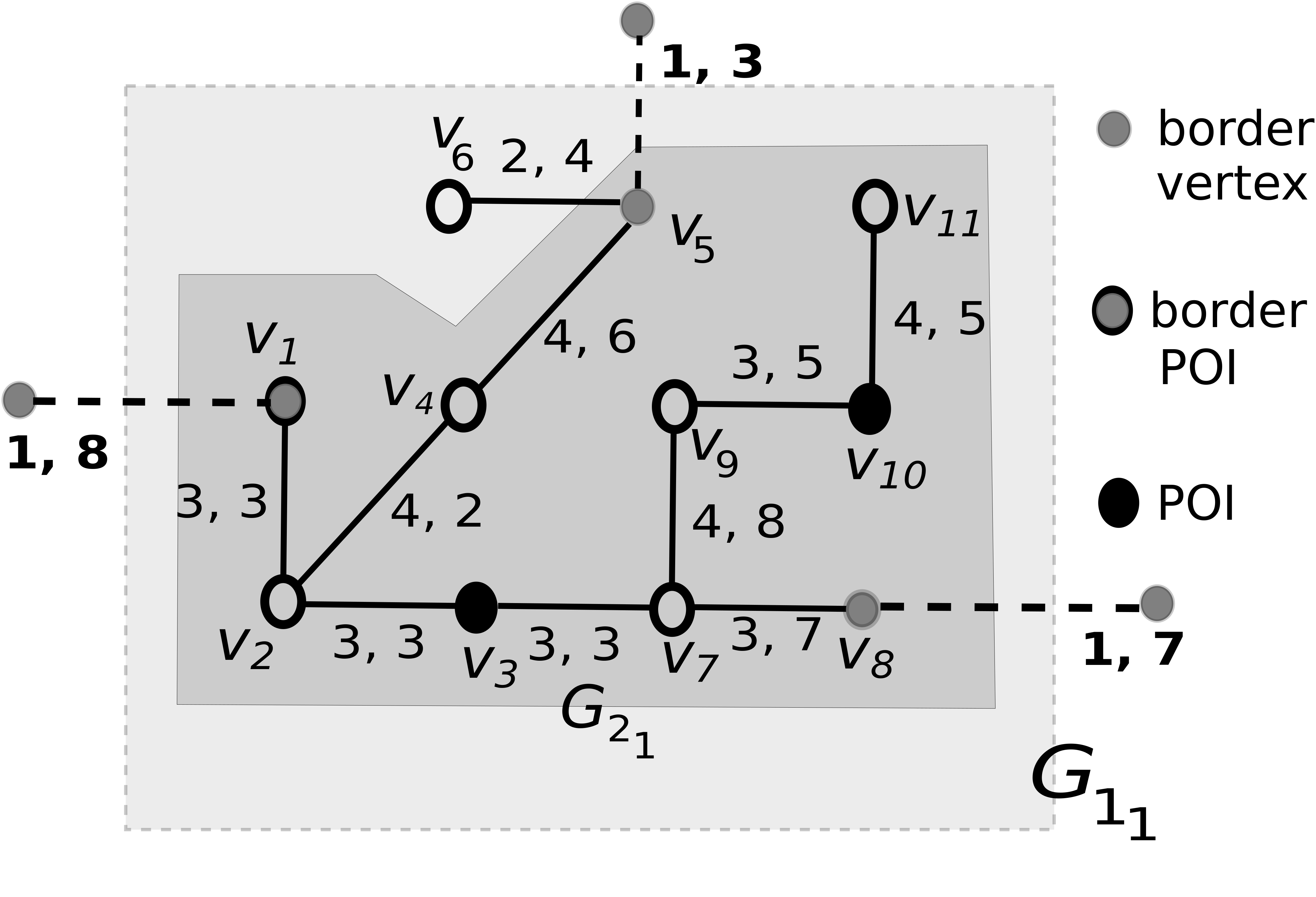
Figure 4: Border vertices, the minimum border distance and the minimum POI distance

Border vertices, the minimum border distance and the minimum POI distance. A vertex $v_{x}$ is called a border vertex of a subgraph $G_{s_{t}}$, if there is an outgoing edge from $v_{x}$ whose ESS is smaller than or equal to $s$ and the edge is not included in $G_{s_{t}}$. We denote the set of border vertices of $G_{s_{t}}$ with $B_{s_{t}}$. For example, in Figure 4, $B_{1_{2}}$ includes $\{v_{1},v_{5},v_{8}\}$. A border vertex of $G_{s_{t}}$ represented by a $Ct$-tree node is also a border vertex of the subgraphs represented by its descendent nodes. For example, $v_{5}$ is a border vertex of both $G_{1_{2}}$ and $G_{2_{1}}$.

For each border vertex, the corresponding $Ct$-tree node stores the minimum border distance and the minimum POI distance. The minimum border distance $d_{B}^{min}(v_{x},G_{s_{t}})$ of a border vertex $v_{x}$ of $G_{s_{t}}$ is defined as the minimum of the distances of the shortest paths from $v_{x}$ to $v_{y}$ for $v_{y}\in B_{s_{t}}\setminus v_{x}$. In Figure 4, the distances of border vertex $v_{8}$ from other border vertices $v_{1}$ and $v_{5}$ are 16 and 21 respectively. Thus, $d_{B}^{min}(v_{8},G_{1_{1}})=16$.

The minimum POI distance $d_{p}^{min}(v_{x},G_{s_{t}})$ of a border vertex $v_{x}$ is defined as is the distance from $v_{x}$ to its closest POI in $G_{s_{t}}$. In Figure 4, the distances of border vertex $v_{8}$ from POIs $v_{1}$, $v_{3}$ and $v_{10}$ are 16, 10 and 20 respectively. Thus, $d_{p}^{min}(v_{8},G_{1_{1}})=10$.

After the $Ct$-tree construction, for each vertex $v$ in $G$, we store a pointer to each $Ct$-tree node whose subgraph contains $v$. Since the height is $s^{max}-1$, this requires adding at most $O(s^{max})$ pointers for each $v$. We remark that the height $h$ of the Ct-tree can be controlled if needed. Specifically, to ensure a height $h$, the domain of possible ESS values is divided in $h$ contiguous intervals and, in each iteration, the edges with ESS in the next smallest interval are removed. E.g., if ESS domain is $1$ to $10$, a Ct-tree of height $5$ can be constructed by first removing edges with ESS in range $(0,2]$ and then $(2,4],(4,6]$ and $(8,10]$ (in this order).

5.2 Query Processing

In Section 5.2.1, we first discuss our technique for $k$ SNN search using the $Ct$-tree properties and in Section 5.2.2, we present the detailed algorithms.

5.2.1 $k$SNN search

The efficiency of any approach for evaluating a $k$SNN query depends on the area of the graph search space for finding the safest paths having distances less than $d_{c}$ from $v_{l}$ to the POIs and the number of POIs considered for identifying $k$SNNs. The $Ct$-tree structure and Property 3 of our PSS measure allow us to start the search from the smallest and safest road network subgraph that has the possibility to include $k$SNNs for $v_{l}$. By construction of $Ct$-tree, it is guaranteed that the subgraph of a child node is smaller and safer than that of its parent node. Thus, starting from the root node, our approach recursively traverses the child nodes that include $v_{l}$. The traversal ends once a child node that includes less than $k$ POIs and $v_{l}$ is reached. The parent of the last traversed child node is selected as the starting node of our $k$SNN search. Note that the subgraph $G_{s_{t}}$ of the starting node includes greater than or equal to $k$ POIs.

If the distances of the paths from $v_{l}$ to at least $k$ POIs in $G_{s_{t}}$ is smaller than $d_{c}$, then our approach does not need to expand $G_{s_{t}}$. This is because, by definition, the edges that connect the border vertices in $G_{s_{t}}$ to other vertices that are not in $G_{s_{t}}$ have lower ESSs than those of the edges in $G_{s_{t}}$. If there are less than $k$ POIs in $G_{s_{t}}$ whose safest paths from $v_{l}$ have distances less than $d_{c}$, our $Ct$-tree based approach recursively updates $G_{s_{t}}$ with the subgragh of its parent node until $k$SNNs are identified.

To find the safest path having distance less than $d_{c}$ from $v_{l}$ to the POIs in $G_{s_{t}}$, we improve the INE based safest path search discussed in Section 4 by incorporating novel pruning techniques using $Ct$-tree properties. Specifically, the minimum border distance and the minimum POI distance stored in the $Ct$-tree node allow us to develop Pruning Rules 3 and 4 to further refine the search space in $G_{s_{t}}$.

Pruning Rule 3

A path $pt_{lj}$ can be pruned if $dist(pt_{lj})+d_{B}^{min}(v_{j},G_{s_{t}})\geq d_{c}$ and $dist(pt_{lj})+d_{p}^{min}(v_{j},G_{s_{t}})\geq d_{c}$, where $v_{j}$ is a border vertex of $G_{s_{t}}$ and $d_{B}^{min}(v_{j},G_{s_{t}})$ and $d_{p}^{min}(v_{j},G_{s_{t}})$ are the minimum border distance and the minimum POI distance of $v_{j}$, respectively.

Pruning Rule 4

A path $pt_{lj}$ can be pruned if $dist(pt_{lj})+d_{B}^{min}(v_{j},G_{s_{t}})\geq d_{c}$ and $dist(pt_{lj})+d_{p}^{min}(v_{j},G_{s_{t}})\geq maxD$, where $v_{j}$ is a border vertex of $G_{s_{t}}$, $P_{s_{t}}$ represents the set of POIs in $G_{s_{t}}$, and $maxD$ represents the maximum of the current shortest distances of the POIs in $P_{s_{t}}$ from $v_{l}$, i.e., $maxD=\max_{p_{i}\in P_{s_{t}}}D_{sh}[i]$.

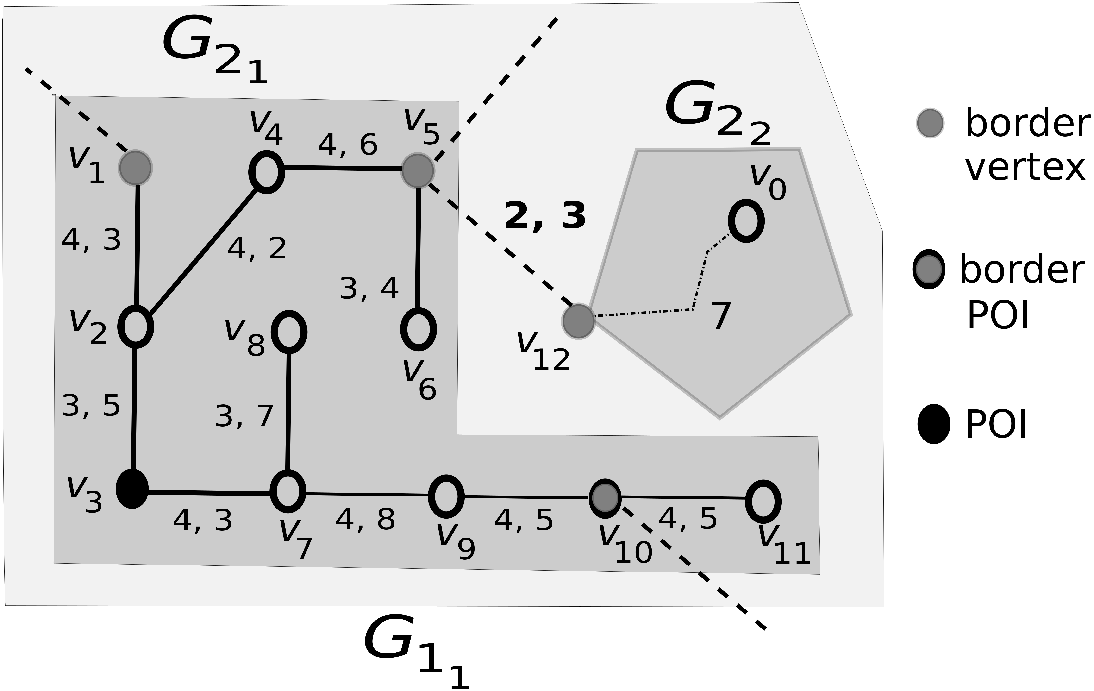
Figure 5: $pt_{05}$ can be pruned using Pruning Rule 3 for a query location $v_{0}$ and $d_{c}=20$

If the first condition that uses the minimum border distance in Pruning Rule 3 or 4 becomes true then it is guaranteed that the expanded path through $pt_{lj}$ cannot cross $G_{s_{t}}$ to reach a POI outside of $G_{s_{t}}$ due to the violation of distance constraint. On the other hand, satisfying the second condition in Pruning Rule 3 means that the expanded path through $pt_{lj}$ cannot reach a POI inside $G_{s_{t}}$ due to the violation of distance constraint. For the second condition, Pruning Rule 4 exploits that if the POIs inside $G_{s_{t}}$ are already reached using other paths then $maxD$, the maximum of the current shortest distances of the POIs in $G_{s_{t}}$ can be used to prune a path. If the second condition in Pruning Rule 4 becomes true then it is guaranteed that the expanded path through $pt_{lj}$ cannot provide paths that are safer than those already identified for the POIs in $G_{s_{t}}$ (please see Pruning Rule 2 for details).

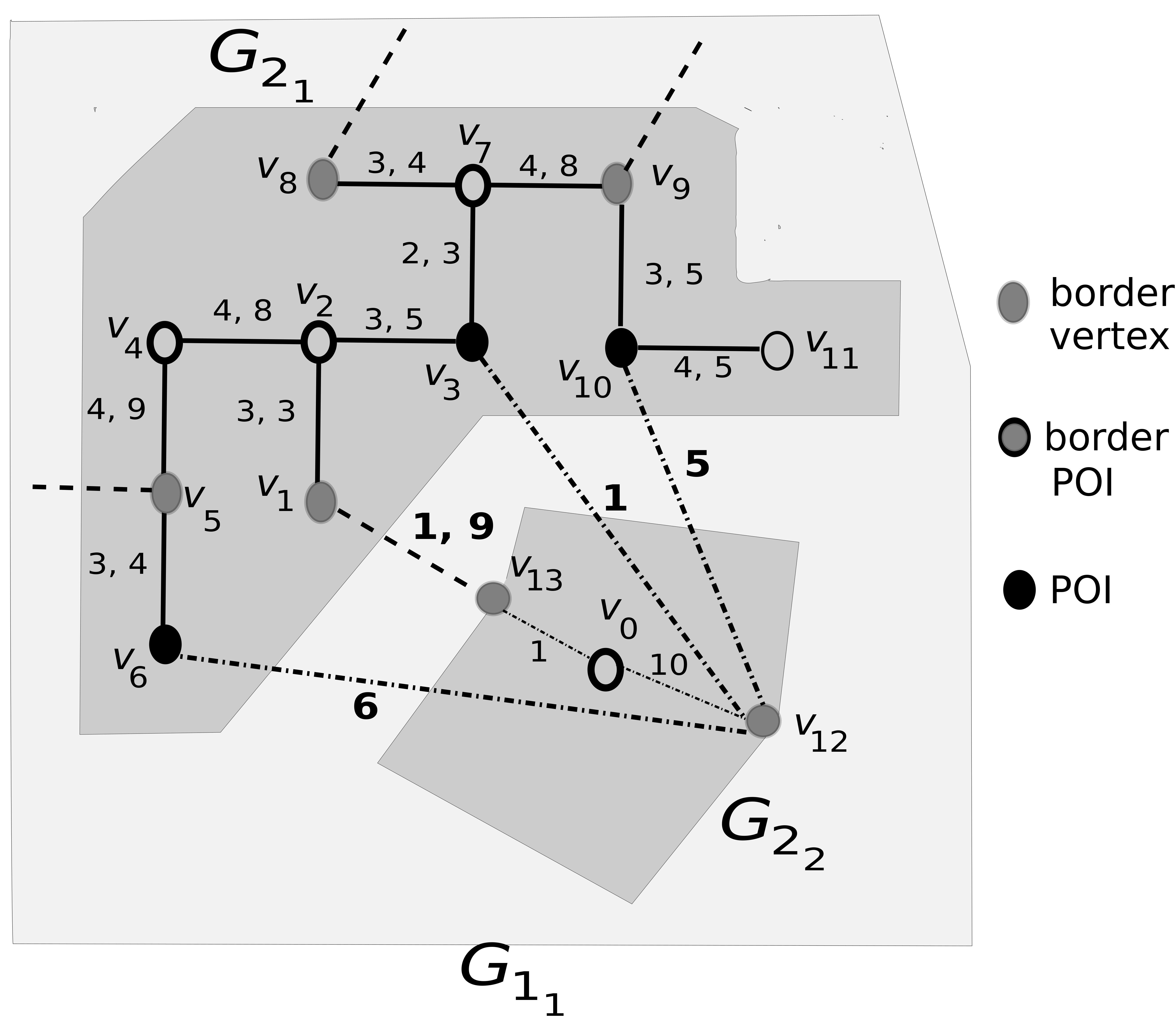
Figure 6: $pt_{01}$ can be pruned using Pruning Rule 4 for a query location $v_{0}$ and $d_{c}=20$

Pruning Rule 4 can prune more paths than Pruning Rule 3 when $maxD$ is less than $d_{c}$, i.e., at least one path from $v_{l}$ to every POI in $G_{s_{t}}$ have been identified. On the other hand, Pruning Rule 3 is better than Pruning Rule 4 when $maxD$ is $\infty$, i.e., no path has yet been identified for a POI in $G_{s_{t}}$. Hence we consider all pruning rules (Pruning Rule 1–Pruning Rule 4) to check whether a path can be pruned.

Figure 5 shows an example where a path $pt_{05}$ is pruned using Pruning Rule 3 for a query location $v_{0}$ and $d_{c}=20$. In the example, $v_{5}$ is a border vertex of $G_{2_{1}}$, $dist(pt_{05})=10$, $d_{B}^{min}(v_{5},G_{2_{1}})=11$ and $d_{p}^{min}(v_{5},G_{2_{1}})=13$. Here, both $dist(pt_{05})+d_{B}^{min}(v_{5},G_{2_{1}})$ and $dist(pt_{05})+d_{p}^{min}(v_{5},G_{2_{1}})$ are greater than $d_{c}$. Hence according to Pruning Rule 3, path $pt_{05}$ can be pruned. From the figure we also observe that if we expand $pt_{05}$, it cannot reach a POI outside $G_{2_{1}}$ through a border vertex ($v_{1}$ or $v_{10}$) or a POI ($v_{3}$ or $v_{10}$) in $G_{2_{1}}$ due to the violation of the distance constraint.

In Figure 6, the POIs ($v_{3}$, $v_{6}$ and $v_{10}$) in $G_{2_{1}}$ are already reached using other paths and $D_{sh}[3]=11$, $D_{sh}[6]=16$ and $D_{sh}[10]=15$. Thus $maxD=16$. The query location is $v_{0}$, $d_{c}=20$, $dist(pt_{01})=10$, $v_{1}$ is a border vertex of $G_{2_{1}}$, $d_{B}^{min}(v_{1},G_{2_{1}})=15$ and $d_{p}^{min}(v_{1},G_{2_{1}})=8$. Here, $dist(pt_{01})+d_{B}^{min}(v_{1},G_{2_{1}})$ is greater than $d_{c}$ and $dist(pt_{01})+d_{p}^{min}(v_{1},G_{2_{1}})$ is greater than $maxD$ but not $d_{c}$. Thus, in this case path $pt_{01}$ is pruned using Pruning Rule 4.

Algorithm 1 $Ct$-tree-$k$SNN($v_{l},k,d_{c}$)

1:  $Initialize(Q_{cur},Q_{next},D_{sh})$

2:  $G_{s_{t}}\leftarrow Contains(v_{l})$

3:  $Enqueue(Q_{cur},v_{l},\infty,0)$

4:  while $Q_{cur}!=\emptyset$ do

5:     $pt_{li},pss(pt_{li}),dist(pt_{li})\leftarrow Dequeue(Q_{cur})$

6:     if  $dist(pt_{li})<D_{sh}[i]$ then

7:        $D_{sh}[i]\leftarrow dist(pt_{li})$

8:     end if

9:     if  $isPOI(v_{i})$ and $!Include(A,v_{i})$ then

10:        $A\leftarrow A\cup\{pt_{li}\}$

11:        if  $A.size()==k$ then

12:           return $A$

13:        end if

14:     end if

15:     if  $v_{i}\in B_{s_{t}}$ then

16:        $Enqueue(Q_{next},pt_{li},pss(pt_{li}),dist(pt_{li}))$

17:     end if

18:     for $e_{ij}\in E_{s_{t}}$ do

19:        if $!PrunePath(pt_{lj},d_{c},D_{sh},G_{s_{t}})$ then

20:           $Enqueue(Q_{cur},pt_{lj},pss(pt_{lj}),dist(pt_{lj}))$

21:        end if

22:     end for

23:     if $Q_{cur}=\emptyset$ then

24:        $G_{s_{t}}\leftarrow GetParent(G_{s_{t}})$

25:        $Q_{cur}\leftarrow Q_{next}$

26:        $Q_{next}\leftarrow\emptyset$

27:     end if

28:  end while

29:  return $A$

5.2.2 Algorithm

Algorithm 1, Ct-$k$SNN, shows the pseudocode to find $k$ SNNs in the road network using the $Ct$-tree index structure. The inputs to the algorithm are $v_{l}$, $k$ and $d_{c}$. The algorithm returns $A$, an array of $k$ entries, where each entry includes the safest path from $v_{l}$ to a POI whose distance is less than $d_{c}$. The entries in $A$ are sorted in the descending order based on the PSS of the safest path.

The algorithm uses two priority queues $Q_{cur}$ and $Q_{next}$, where $Q_{cur}$ is used for the path expansion in $G_{s_{t}}$, and $Q_{next}$ stores the paths that will be expanded WHILE searching the parent subgraph of $G_{s_{t}}$. Each entry of these queues represents a path, the PSS and the path’s length. The entries in a queue are ordered in descending order based on their PSSs. The algorithm uses an array $D_{sh}$, where $D_{sh}[i]$ stores the distance of the shortest dequeued path from $v_{l}$ to $v_{i}$.

The algorithm starts with initializing two priority queues $Q_{cur}$ and $Q_{next}$ to $\emptyset$ and $D_{sh}[i]$ for each $v_{i}$ to $d_{c}$ using Function $Initialize$ (Line 1). Then, starting from the root node, Function $Contains$ recursively traverses the child nodes using the stored pointers of $v_{l}$ until it identifies the smallest subgraph $G_{s_{t}}$ of a $Ct$-tree node that includes $v_{l}$ and has at least $k$ POIs (Line 2). The $v_{l}$ and the corresponding path information are enqueued to $Q_{cur}$. The algorithm iteratively processes the entries in $Q_{cur}$ until it becomes empty or $k$SNNs are found (Lines 4–28).

In every iteration, the algorithm dequeues a path $pt_{li}$ from $Q_{cur}$ and updates $D_{sh}[i]$ of the last vertex $v_{i}$ of the dequeued path if $dist(pt_{li})<D_{sh}[i]$ (Lines 5–8). If $v_{i}$ represents a POI that is not already present in $A$, then $pt_{li}$ is added to $A$, and if $A$ includes $k$ entries, the answer is returned (Lines 9–14).

If $v_{i}$ is a border vertex of $G_{s_{t}}$, then there is at least one outgoing edge from $v_{i}$ with safety score smaller than or equal to $s$, which might need to be later considered if $k$SNNs are not found in current $G_{s_{t}}$. Thus, $pt_{li}$ and the corresponding path information are enqueued to $Q_{next}$ (Lines 15–17). Note that the ESS of $G_{s_{t}}$ are larger than $s$.

Next, for each outgoing edge $e_{ij}$ of $v_{i}$ in $G_{s_{t}}$, the algorithm checks whether the newly formed path $pt_{lj}$ by adding $e_{ij}$ at the end of $pt_{li}$ can be pruned using $PrunePath$ function ($PrunePath$ is elaborated below). If the path is not pruned, then $pt_{lj}$ and the corresponding path information are enqueued to $Q_{cur}$ (Lines 18–22).

At the end of the iteration, the algorithm checks whether the exploration of $G_{s_{t}}$ is complete, i.e., $Q_{cur}$ is empty. If this condition is true, then it means that the safest paths having distances less than $d_{c}$ from $v_{l}$ to $k$SNNs are not included in $G_{s_{t}}$. Thus, the algorithm sets the parent of $G_{s_{t}}$ as $G_{s_{t}}$, assigns $Q_{next}$ to $Q_{cur}$ and resets $Q_{next}$ to $\emptyset$ (Lines 23-27).

PrunePath. Algorithm 2 returns $true$ if path $pt_{ij}$ can be pruned by any of our pruning criteria and $false$ otherwise. The algorithm first checks whether $pt_{ij}$ can be pruned using the criteria in Pruning Rules 1 or 2. Note that an entry $D_{sh}[x]$ for a vertex $v_{x}$ is initialized to $d_{c}$ and later it gets updated once a path to $v_{x}$ is dequeued from the queue (see Line 7 in Algorithm 1).

If $pt_{ij}$ is not pruned, Function $checkBorder(G_{s_{t}},v_{j})$ checks whether $v_{j}$ is a border vertex of $G_{s_{t}}$ or one of its descendants. If so, it returns $true$ for $IsBorder$ and the node $G_{{s^{\prime}}_{t^{\prime}}}$ for which $v_{j}$ is a border vertex. Otherwise, $IsBorder$ is set to $false$. By construction of the $Ct$-tree, a border vertex of a $Ct$-tree node is also the border vertex of its descendants. Thus, there may be multiple nodes for which $v_{j}$ is a border vertex, in which case, $G_{{s^{\prime}}_{t^{\prime}}}$ is chosen to be the highest node in the $Ct$-tree for which $v_{j}$ is a border vertex.

If $v_{j}$ is a border vertex then the algorithm checks whether $pt_{ij}$ can be pruned using Pruning Rules 3 or 4 (Lines 5–8). One of the pruning condition that uses the minimum border distance is same in both Pruning Rules 3 and 4, which is checked in Line 5. The left part of the other condition, adding the minimum POI distance with $dist(pt_{ij})$ is also same in both pruning rules. The right part is $d_{c}$ for Pruning Rule 3 and $maxD$ for Pruning Rule 4, where $maxD$ represents the maximum of the current shortest distances of $v_{l}$ to the POIs in $G_{{s^{\prime}}_{t^{\prime}}}$. The shortest distance of every vertex (including POIs) is initialized to $d_{c}$ (Line 1 of Algorithm 1). Thus, $maxD$ is initially $d_{c}$ and later may become less than $d_{c}$ when the paths to POIs in $G_{{s^{\prime}}_{t^{\prime}}}$ are dequeued from the priority queue (Lines 5–7 of Algorithm 1).

Since the minimum border distance and minimum POI distance of a $Ct$-tree node are greater than or equal to those of its descendants, it is not required to check these pruning conditions for $v_{j}$ for the descendants of $G_{{s^{\prime}}_{t^{\prime}}}$ separately.

Algorithm 2 $PrunePath(pt_{lj},d_{c},D_{sh},G_{s_{t}})$

1:  if $dist(pt_{lj})\geq D_{sh}[j]$ then

2:     return true

3:  end if

4:  $isBorder{G_{{s^{\prime}}_{t^{\prime}}}}\leftarrow checkBorder(G_{s_{t}},v_{j})$

5:  if $isBorder==true$ and $dist(pt_{lj})+d_{B}^{min}(v_{j},G_{{s^{\prime}}_{t^{\prime}}})\geq d_{c}$ then

6:     if $dist(pt_{lj})+d_{p}^{min}(v_{j},G_{{s^{\prime}}_{t^{\prime}}})\geq maxD$ then

7:        return  true

8:     end if

9:  end if

10:  return  false

Complexity Analysis. Since the height $h$ of the $Ct$-tree is bounded by $s^{max}-1$, the $Contains$ function (Line 2, Algorithm 1) to obtain intial $G_{s_{t}}$ takes $O(s^{max})$, where $s^{max}$ is typically a small constant (e.g., 5, 10 or 15). To expand search range and update $G_{s_{t}}$, Function $GetParent$ is called at most $(s^{max}-1)$ times and thus, its overall worst case time complexity is also $O(s^{max})$.

Let the total number of valid paths from $v_{l}$ to any node in $G_{s_{t}}$ be $n^{\prime}_{p}$. Then the worst case time complexity for finding $k$ SNNs by applying the INE based search using a priority queue is $O(n^{\prime}_{p}\log(n^{\prime}_{p}))$. The number of total paths reduces when we apply Pruning Rules 2, 3, and 4. Let $r^{\prime}$ be the combined effect factor of these three pruning rules. Thus, by applying the pruning rules, the worst case time complexity of the INE based search in $G_{s_{t}}$ becomes $O(\frac{n^{\prime}_{p}}{r^{\prime}}\log(\frac{n^{\prime}_{p}}{r^{\prime}}))$. Thus, the worst case time complexity for the $Ct$-tree based approach is $O(s^{max}+\frac{n^{\prime}_{p}}{r^{\prime}}\log(\frac{n^{\prime}_{p}}{r^{\prime}}))$. Note that this complexity is significantly better than the worst case time complexity of INE-based approach because $s^{max}$ is typically a small constant, $n^{\prime}_{p}/r^{\prime}$ is significantly smaller than $n_{p}/r$ because $G_{s_{t}}\subseteq G$ and $Ct$-tree uses additional pruning rules.

5.3 Ct-tree Update

A $Ct$-tree needs an update when there is any change in the edges or POIs of the road network.

Adding/removing an edge or change in ESS When an edge $e_{xy}$ with ESS $s$ is added/removed, the $Ct$-tree nodes whose subgraphs allow ESS $s$ and include $v_{x}$ and/or $v_{y}$ may get affected. If $v_{x}$ and $v_{y}$ are located at different subgraphs then two subgraphs become connected when $e_{xy}$ is added and their corresponding $Ct$-tree nodes are merged into one. On the other hand, the removal of $e_{xy}$ from a subgraph may divide the subgraph into two components and the corresponding $Ct$-tree node to two nodes. This process recursively continues by checking the child nodes that include $v_{x}$ and/or $v_{y}$ until the subgraphs whose allowed ESS is greater than $s$ is reached.

When an ESS changes, the ESS is simply updated in the subgraphs where the edge already exists. If an ESS increases (e.g., ESS increases from 3 to 4), the edge is added to the subgraphs, where the new ESS is allowed. On the other hand, If an ESS decreases (e.g., ESS decreases to 3 from 4), the edge is removed from the subgraphs where the new ESS is not allowed. The addition or removal of an edge may result in the merge or division of the subgraph(s) and their corresponding $Ct$-tree node(s).

Although the travel time associated with a road represented by an edge may change frequently, the changes in ESS values are not frequent, e.g., the ESS may decrease when there is a reported crime on the edge. Also, in most real world applications, the updates to ESSs are periodic (e.g., all ESS values may be updated at the end of every week based on the recent crime data). Even if an ESS changes, the change normally happens in small step (e.g., 5 to 4). It is an uncommon scenario that an ESS suddenly changes from 5 to 1. As a result the update process due to an ESS change affect only a small portion of the $Ct$-tree structure and incurs low processing overhead.

Adding/removing a POI: When a POI is added or removed, the information on the number of POIs stored in the $Ct$-tree nodes are updated accordingly.

Irrespective of the $Ct$-tree structure update, adding/removing an edge $e_{xy}$ or a change in the ESS of $e_{xy}$ or adding/removing a POI may require update in the border vertex set, the minimum border distance, the minimum POI distance of border vertices for the $Ct$-tree nodes whose subgraphs include $v_{x}$ and/or $v_{y}$ and the stored pointers to the $Ct$-tree nodes for the vertices in the road network graph.

6 Safety Score Based Network Voronoi Diagram

The concept of the network Voronoi diagram (NVD) OkabeBSCK00 ; OkabeSFSO08 has been shown as an effective method for faster processing of $k$ nearest neighbor queries KolahdouzanS04 ; SafarET09 . The traditional NVD is computed based on distance and does not apply for processing $k$SNN queries. In Section 6.1, we introduce safety score based network Voronoi diagram (SNVD) and present its properties.

We develop an efficient technique to compute the $k$SNNs using the SNVD. Our solution is composed of two phases: preprocessing and query processing. In Sections 6.2 and 6.3, we elaborate the preprocessing steps and the query processing algorithm, respectively. In Section 6.4, we discuss how to update the SNVD for a change in the road network.

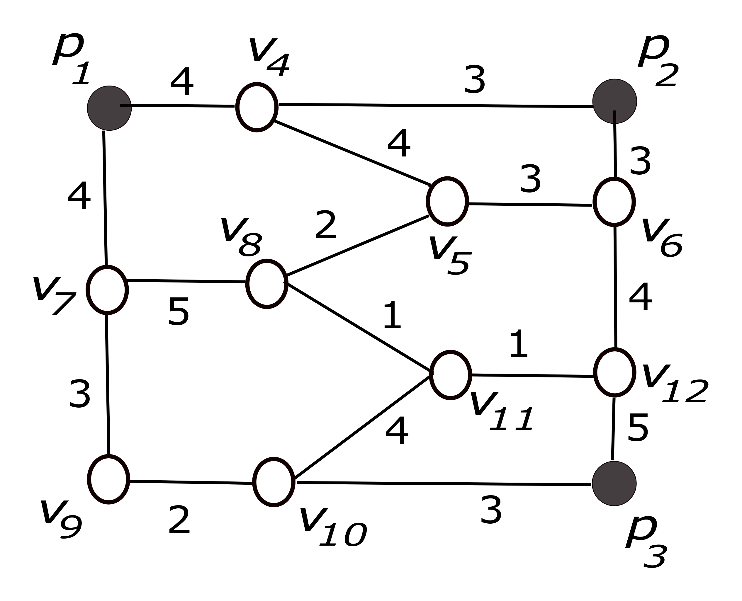
(a) Original Graph	(b) SNVD

Figure 7: An example of SNVD

6.1 SNVD Properties

An SNVD divides the road network graph into subgraphs such that each subgraph contains a single POI which is the unconstrained safest neighbor for every point of the subgraph. We differentiate the unconstrained safest neighbor from the safest nearby neighbor (SNN) by considering unconstrained safest path. For an unconstrained safest path, we assume a sufficiently large value for $d_{c}$ such that every simple path in the graph has length less than $d_{c}$, e.g., $d_{c}$ is just bigger than the sum of the lengths of all edges in the graph. The subgraphs are called Voronoi cells and a point that defines the boundary between two adjacent Voronoi cells is a called a border vertex. The Voronoi cell of POI $p_{i}$ is denoted as ${VC}_{i}$ and the border vertex set for ${VC}_{i}$ is denoted as $B_{i}$.

Figure 7 shows an example of an SNVD. Black vertices represent the generator POIs $p_{1}$, $p_{2}$ and $p_{3}$, white vertices represent the road intersections, and grey vertices represent the border vertices.

Figure 8: Example border vertices of an SNVD, weights associated with each edge are $w_{ij}^{ss}$, $w_{ij}^{d}$, respectively

Unlike traditional distance based NVD SafarET09 ; XuanZTSSG09 , a border vertex $b$ between two adjacent Voronoi cells ${VC}_{i}$ and ${VC}_{j}$ may not have equal PSS for its unconstrained safest paths to $p_{i}$ and $p_{j}$. Figure 8 shows examples of such scenarios. When the PSSs for $b$’s unconstrained safest paths to $p_{i}$ and $p_{j}$ differ, the unconstrained safest neighbor of $b$ is one of the POIs $p_{i}$ and $p_{j}$ for which $b$ has the higher PSS.

The following lemmas shows the properties of SNVD that we exploit in our solution.

Lemma 3

Let $p_{1},p_{2},\dots,p_{k-1}$ represent the $k-1$ unconstrained safest POIs of $v_{l}$, respectively. The unconstrained safest path from $v_{l}$ to its $k^{th}$ unconstrained safest POI $p_{k}$ can only go through $\{{VC}_{1},{VC}_{2},\dots,{VC}_{k-1},{VC}_{k}\}$.

Proof

Assume that the unconstrained safest path from $v_{l}$ to $p_{k}$ goes through a vertex $v$ of ${VC}_{t}$, where $t\notin\{1,2,\dots,k\}$. By construction of SNVD, POI $p_{t}$ is safer than POI $p_{k}$ for $v$. Since the unconstrained safest path from $v_{l}$ to $p_{k}$ goes through $v$, POI $p_{t}$ is also safer than POI $p_{k}$ for $v_{l}$. Thus $t\in\{1,2,\dots,k\}$, which contradicts our assumption. ∎

Lemma 4

Let $v_{1},v_{2},\dots,v_{k-1}$ represent the $k-1$ unconstrained safest POIs of $v_{l}$, respectively. The $k^{th}$ unconstrained safest POI $p_{k}$ of $v_{l}$ lies in one of the adjacent Voronoi cells of ${VC}_{1},{VC}_{2},\dots,{VC}_{k-1}$.

Proof

If the $k^{th}$ unconstrained safest POI $v_{k}$ of $v_{l}$ does not lie in one of the adjacent Voronoi cells of ${VC}_{1},{VC}_{2},\dots,{VC}_{k-1}$, then the unconstrained safest path between $v_{l}$ and $v_{k}$ must go through a vertex which does not lie in ${VC}_{1},{VC}_{2},\dots,{VC}_{k-1},{VC}_{k}$, which contradicts Lemma 3. Thus, the $k^{th}$ unconstrained safest POI of $v_{l}$ lies in one of the adjacent Voronoi cells of ${VC}_{1},{VC}_{2},\dots,{VC}_{k-1}$. ∎

6.2 Prepossessing

The following information will be precomputed and stored for the faster processing of $k$SNN queries:

• Voronoi cells, where each Voronoi cell ${VC}_{i}$ has the POI $p_{i}$ as the generator, a set $B_{i}$ of border vertices, and a list $L_{i}$ of pointers to adjacent Voronoi Cells

• For every vertex $v\in B_{i}$, the unconstrained safest path between $v$ and $p_{i}$ and its PSS

• For every pair of border vertices $v_{i}\in B_{i}$ and $v_{j}\in B_{i}$, the unconstrained safest path between $v_{i}$ and $v_{j}$ that lies completely inside $VC_{i}$ and its PSS

• For every $v_{x}\in B_{i}$ the minimum border distance and the minimum POI distance, where the minimum border distance of a border vertex is defined as $argmin_{v_{y}\in B_{i}\setminus v_{x}}dist(pt^{sh}_{xy})$ and the minimum POI distance is $dist(pt^{sh}_{xi})$ and the shortest paths for the minimum border distance and the minimum POI distance are computed by considering only the subgraph represented by Voronoi cell ${VC}_{i}$

• For every vertex $v$ in the road network graph $G$, a pointer to the Voronoi cell whose POI generator is the unconstrained safest neighbour of $v$

To construct the SNVD, we first apply parallel Dijkstra algorithm Erwig00 to find the unconstrained safest POI for each vertex in the road network. Starting from a start vertex, the Dijkstra algorithm keeps track of the unconstrained safest path for every visited vertex. When the distance for the safest path is unconstrained, no path gets pruned and thus unlike INE, it is sufficient to only expand the unconstrained safest path from a vertex.

Then we compute the border vertices as follows: (i) if the unconstrained safest paths from $v$ to two POIs $p_{i}$ and $p_{j}$ have the same PSS, then $v$ is considered as a border vertex of Voronoi cells ${VC}_{i}$ and ${VC}_{j}$, and (ii) if two end vertices of an edge have different unconstrained safest POIs, say $p_{i}$ and $p_{j}$, and the ESS associated with the edge is $s$, then the point $b$ of the edge that provides equal distance associated with $s$ in both of the $b$’s safest paths to $p_{i}$ and $p_{j}$ is identified as a border vertex of Voronoi cells ${VC}_{i}$ and ${VC}_{j}$. Figure 8 shows three example scenarios. In case 1, the end vertices of the edge with ESS 1 has different unconstrained safest POIs and the distance of the edge is 4. There is no other edge in $pt_{ij}$ with ESS 1. Thus $b$ is placed at the midpoint of the edge so that both of the $b$’s safest paths to $p_{i}$ and $p_{j}$ have equal distance for ESS 1. For case 2, $b$ is not the midpoint of the edge as there is another edge in $pt_{ij}$ with ESS 1. Note that in case 3, $b$ is placed at the mid of the edge with ESS 2, which is not the minimum ESS in $pt_{ij}$. This is because both of the $b$’s safest paths to $p_{i}$ and $p_{j}$ already have an edge with the same distance for ESS 1.

The resulted distances of the splitted edges with a border vertex $b$ may become less than 1. This occurs when the length of the edge that is splitted by $b$ is 1 and no other edge in $pt_{ij}$ has the same ESS as the splitted edge. Our PSS measure requires the edge weight to be greater than or equal to 1. Thus, after the construction of the whole SNVD, if the distance of any splitted edge becomes less than 1, we scale up the distances of all edges in the road network to ensure that the distances of the splitted edges are greater than or equal to 1 and recompute the SNVD.

To compute the unconstrained safest path between $v_{i}$ and $v_{j}$ that lies completely inside $VC_{i}$ for every pair of border vertices $v_{i}\in B_{i}$ and $v_{j}\in B_{i}$, we apply Dijkstra algorithm within $VC_{i}$.

6.3 Query Processing

According to the construction of SNVD, a POI $p_{i}$ is the unconstrained safest neighbor for every location $v$ in a Voronoi cell $VC_{i}$. However, an unconstrained safest neighbor is not necessarily the SNN for a location $v$ if the distance of the unconstrained safest path from $v$ to $p_{i}$ is greater than or equal to the distance constraint $d_{c}$ specified in the query. Hence, unlike the existing NVD based nearest neighbor search algorithms KolahdouzanS04 , we cannot simply return the POI of the Voronoi cell that includes the query location as the SNN. Since $d_{c}$ is a query specific parameter, it is also not possible to consider $d_{c}$ while computing the Voronoi cells of the SNVD. In Sections 6.3.1, we discuss our SNVD based solution to find $k$SNNs and in Section 6.3.2, we elaborate our efficient (unconstrained and constrained) safest path computation techniques by exploiting SNVD properties.

6.3.1 kSNN search

Our SNN search technique using SNVD incrementally finds the unconstrained safest neighbors and adds each of these neighbors in a candidate set. The incremental search stops when the candidate set contains at least $k$ POIs that have unconstrained safest paths with length less than $d_{c}$. Let $k+m$ be the size of the candidate set where $m\geq 0$. The k SNNs are guaranteed to be among the candidate set. Then, we compute the PSSs of the safest paths from $v_{l}$ to the remaining $m$ POIs in the candidate set to determine the query answer. The POIs whose safest paths from $v_{l}$ among $k+m$ candidates have $k$ largest PSSs and have distances less than $d_{c}$ are identified as $k$SNNs.

Algorithm 3 shows the steps to find $k$SNNs in the road network using the SNVD. The inputs to the algorithm are $v_{l}$, $k$ and $d_{c}$. The algorithm initializes $it$ and $j$ to 1, finds the first unconstrained safest neighbor using the stored pointer (Function $FindUSN$) and adds it to the candidate POI set $C_{P}$ (Lines 1–2). Then the algorithm iterates in a loop until $C_{P}$ includes $k$SNNs. In every iteration, the algorithm checks whether the distance of the unconstrained safest path from $v_{l}$ to the $j^{th}$ unconstrained safest neighbor is less than $d_{c}$. If yes, Function $IsConstrained$ returns true and $it$ is incremented by 1 (Lines 4–6)). At the end of the iteration, the algorithm increments $j$ by 1 and finds the next ($j^{th}$) unconstrained safest neighbor using Function $NextUCN$ (Lines 7–8). When the loop ends, $FindA$ identifies the answer of the $k$SNN query in $A$ (Line 10).

Algorithm 3 SNVD-$k$SNN($v_{l},k,d_{c}$)

1:  $it,j\leftarrow 1$

2:  $C_{P}\leftarrow FindUSN(v_{l})$

3:  while $it\leq k$ do

4:     if $IsConstrained(C_{P},j,d_{c})$ then

5:        $it\leftarrow it+1$

6:     end if

7:     $j\leftarrow j+1$

8:     $C_{P}\leftarrow C_{P}\cup NextUSN(v_{l},j)$

9:  end while

10:  $A\leftarrow FindA(A,C_{P})$

11:  return  $A$

Incremental computation of unconstrained safest neighbors. Function $FindUSN$ locates Voronoi cell ${VC}_{q}$ that includes $v_{l}$ and returns the corresponding POI $p_{q}$ as the first unconstrained safest neighbor. ${VC}_{q}$ becomes the first candidate Voronoi cell of the set $C_{VC}$. To compute the second unconstrained safest neighbor, Function $NextUSN$ adds the adjacent Voronoi cells of ${VC}_{q}$ to $C_{VC}$ as they include the second unconstrained safest POI of $v_{l}$ (Lemma 4). The POI of one of these candidate Voronoi cells in $C_{VC}$ whose unconstrained safest path to $v_{l}$ has the second best PSS is identified as the second unconstrained safest neighbor of $v_{l}$ (please see Section 6.3.2 for unconstrained safest path computation technique). Similarly, to find the $j^{th}$ unconstrained safest neighbor of $v_{l}$, $NextUSN$ adds the adjacent Voronoi cells of the $(j-1)^{th}$ unconstrained safest neighbor’s Voronoi cell in $C_{VC}$, if they are not already included in $C_{VC}$. The $j^{th}$ unconstrained safest neighbor of $v_{l}$ is the POI that has the $j^{th}$ best PSS for the unconstrained safest path from $v_{l}$ among the POIs of the candidate Voronoi cells.

6.3.2 Safest Path Computation

Our PSS measure and the property shown in Lemma 3 allow us to adapt the shortest path computation technique proposed in KolahdouzanS04 for finding the unconstrained safest paths from $v_{l}$ to a POI of the candidate Voronoi cell in $C_{VC}$. After $FindUSN$ locates Voronoi cell ${VC}_{q}$ that includes $v_{l}$, it computes the unconstrained safest paths from $v_{l}$ to $p_{q}$ and the border vertices of $VC_{q}$ using Dijkstra algorithm. Then similar to KolahdouzanS04 , we use precomputed unconstrained safest paths between border vertices for this purpose and reduce the processing overhead significantly. In experiments, we show that the number of border vertices of an SNVD is small with respect to the total number of vertices and thus, the overhead for storing the unconstrained safest paths for the border vertices is negligible.

On the other hand, we cannot use precomputed unconstrained safest paths and adapt KolahdouzanS04 to compute the safest path between $v_{l}$ and a POI while identifying $k$SNNs from candidate $k+m$ POIs. We improve the INE based safest path search technique discussed in Section 4 by incorporating novel pruning techniques for search space refinement using SNVD properties and apply it to compute the safest paths that have distances less than $d_{c}$. Pruning Rules 5 and 6 use the minimum border distances and minimum POI distances of the border vertices, respectively, in the pruning condition:

Pruning Rule 5

Let the safest path between $v_{l}$ and POI $p_{y}$ needs to be determined. A path $pt_{lj}$ can be pruned if $dist(pt_{lj})+d_{B}^{min}(v_{j},{VC}_{x})\geq d_{c}$, where $v_{j}$ is a border vertex of Voronoi cell ${VC}_{x}$, $d_{B}^{min}(v_{j},{VC}_{x})$ represents the minimum border distance of $v_{j}$ and $d_{c}$ represent the distance constraint.

Pruning Rule 6

Let the safest path between $v_{l}$ and POI $p_{x}$ needs to be determined. A path $pt_{lj}$ can be pruned if $dist(pt_{lj})+d_{p}^{min}(v_{j},{VC}_{x})\geq d_{c}$, where $v_{j}$ is a border vertex of Voronoi cell ${VC}_{x}$, $d_{p}^{min}(v_{j},{VC}_{x})$ represents the minimum POI distance of $v_{j}$ and $d_{c}$ represent the distance constraint.

We have $s_{k}$, the upper bound of the PSS of the safest path between $v_{l}$ and its $k^{th}$ SNN, once $k$ unconstrained safest neighbors of $v_{l}$ that have distances less than $d_{c}$ from $v_{l}$ are identified. Later if a safest path from $v_{l}$ to a new POI is identified that has the distance less than $d_{c}$ and PSS higher than current $s_{k}$, then $s_{k}$ is updated to the new PSS. By exploiting the property that the PSS of a subpath is higher than that of the path (Property 2) and $s_{k}$, we develop a new pruning technique as follows:

Pruning Rule 7

A path $pt_{lj}$ can be pruned if $pss(pt_{lj})<s_{k}$, where $s_{k}$ represent the upper bound of the PSS of the safest path between $v_{l}$ and its $k^{th}$ SNN.

Thus, in addition to Pruning Rules 1 and 2, our SNVD based solution checks whether a path can be pruned using Pruning Rules 5, 6 and 7 to find the safest paths that have distances less than $d_{c}$.

Complexity Analysis. Function $FindUSN$ identifies the unconstrained safest neighbor $p_{q}$ of $v_{l}$ in $O(1)$ using the pointer for each vertex storing its Voronoi generator. $FindUSN$ also computes the unconstrained safest paths from $v_{l}$ to $p_{q}$ and the border vertices of $VC_{q}$ using Dijkstra algorithm with the worst case time complexity $O(E_{q}\log(V_{q}))$ where $E_{q}$ is the number of edges in $VC_{q}$. The loop (Lines 3–9) iterates $(k+m)$ times. In the $j^{th}$ iteration, Function $isConstrained$ checks whether the distance of the unconstrained safest path from $v_{l}$ to the $j^{th}$ unconstrained safest nearest neighbour is smaller than $d_{c}$ in constant time. Function $NextUSN$ incrementally finds $(j+1)^{th}$ unconstrained safest neighbor of $v_{l}$ using precomputed distances and stored lists of neighbor SNVD cells. Thus, the overall time complexity of the loop for $(k+m)$ iterations is $O(k+m)$. The parameter $m$ is typically a small value (e.g., around 8 in our experimental study).

Function $FindA$ needs to compute the safest paths that have distances less than $d_{c}$ from $v_{l}$ to $m$ POIs. Let $n^{\prime\prime}_{p}$ be the total number of valid paths from $v_{l}$ to any node in the Voronoi cells of the $(k+m)$ POIs. Then, the worst case time complexity for finding these safest paths by applying the INE based search using a priority queue is O($n^{\prime\prime}_{p}$ $\log(n^{\prime\prime}_{p})$). The number of total paths reduces when we apply Pruning Rules 2, 4, 5, 6 and 7. Let $r^{\prime\prime}$ be the combined effect factor of these pruning rules. By applying the pruning rules the worst case time complexity of the INE based search becomes $O(\frac{n^{\prime\prime}_{p}}{r^{\prime\prime}}\log(\frac{n^{\prime\prime}_{p}}{r^{\prime\prime}}))$. Thus, the worst case time complexity for the SNVD based approach is $O(k+m+E_{q}\log(V_{q})+\frac{n^{\prime\prime}_{p}}{r^{\prime\prime}}\log(\frac{n^{\prime\prime}_{p}}{r^{\prime\prime}}))$. It can be shown that the cost of finding the $m$ safest paths $O(\frac{n^{\prime\prime}_{p}}{r^{\prime\prime}}\log(\frac{n^{\prime\prime}_{p}}{r^{\prime\prime}}))$ dominates the cost of Dijksra’s search $O(E_{q}\log{(V_{q})})$ because the search space to find the $m$ safest paths is larger than $VC_{q}$. Thus, the worst case complexity is $O(k+m+\frac{n^{\prime\prime}_{p}}{r^{\prime\prime}}\log(\frac{n^{\prime\prime}_{p}}{r^{\prime\prime}}))$ which is significantly better than the worst case time complexity of INE based approach because $k+m$ is quite small in practice and $n^{\prime\prime}_{p}/r^{\prime\prime}$ is significantly smaller than $n_{p}/r$.

6.4 SNVD Update

An SNVD needs to be updated when there is any change in the edges or POIs of the road network. These changes only have effect on their local neighborhood and thus, the SNVD does not need to be reconstructed from scratch.

Adding/removing an edge or a change in the edge safety score: When an edge is added or removed or if the ESS changes, we first identify the Voronoi cell $VC$ where the edge is located. Then for every border vertex of $VC$, we recompute the unconstrained safest path between the border vertex and the POI of the Voronoi cell. Any change in the PSS of an unconstrained safest path may require shifting the border vertex location. If the location of a border vertex changes then the adjacent Voronoi cell that also shares the border vertex gets affected. After reconstructing the affected Voronoi cells, we also update their stored information (e.g., the minimum border distance for a border vertex may change for removing an edge).

Adding/removing a POI: When a POI is added or removed, we need to first identify the Voronoi cell $VC_{x}$, where the POI is located. If the POI is removed, the subgraph represented by $VC_{x}$ is merged with its adjacent Voronoi cells. On the other hand, if a new POI is added then $VC_{x}$ is divided into two new Voronoi cells and their adjacent Voronoi cells may also get affected. In both cases, we reconstruct the affected Voronoi cells and update their stored information.

7 Experiments

We propose novel algorithms, $Ct$-tree-$k$SNN and SNVD-$k$SNN using a $Ct$-tree and an SNVD, respectively for finding the safest nearby POIs. There is no existing work to compute $k$SNNs and thus, in this paper, we compare $Ct$-tree-$k$SNN and SNVD-$k$SNN against two baselines: $R$-tree-$k$SNN and INE-$k$SNN. $R$-tree-$k$SNN, indexes POIs using an $R$-tree and uses techniques in HjaltasonS99 to find the candidate $k$SNN POIs whose Euclidean distances from the query location are less than $d_{c}$. Then, $R$-tree-$k$SNN applies techniques in Islam21 to find the safest valid paths to these candidate POIs to determine the $k$SNNs. INE-$k$SNN is the extension of INE for evaluating $k$SNN queries (Section 4).

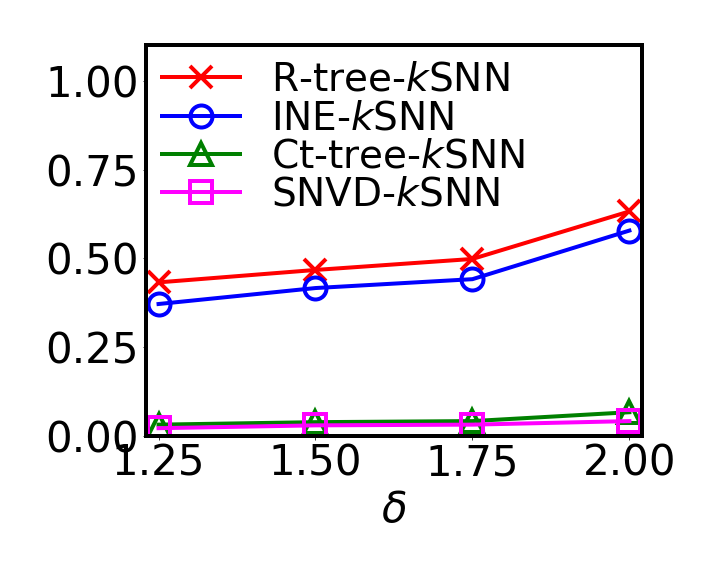
(a) CH	(b) PHL	(c) SF
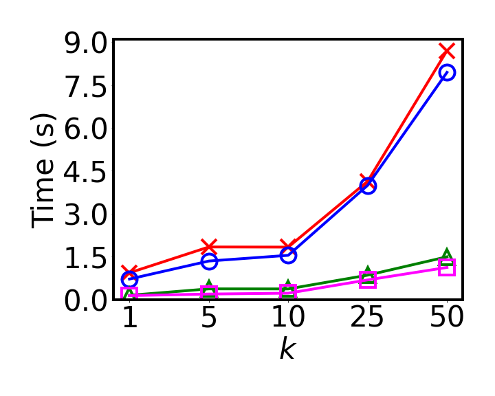
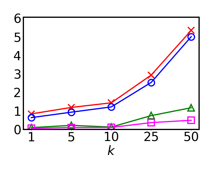
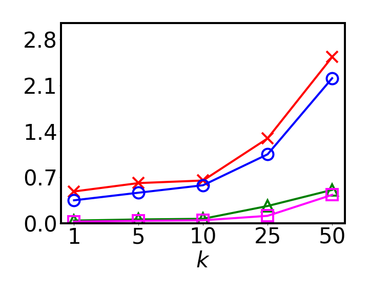
(d) CH	(e) PHL	(f) SF
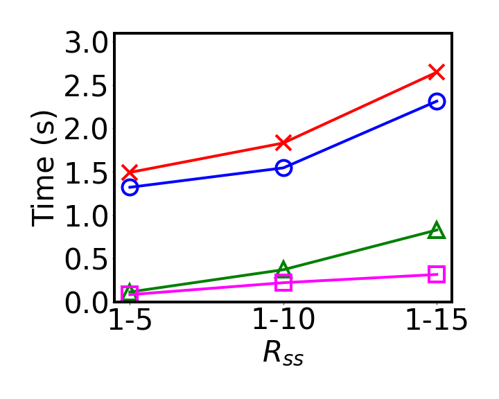
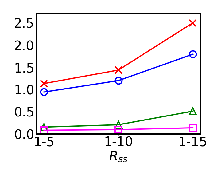
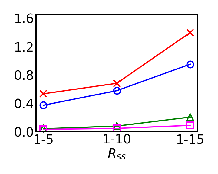
(g) CH	(h) PHL	(i) SF
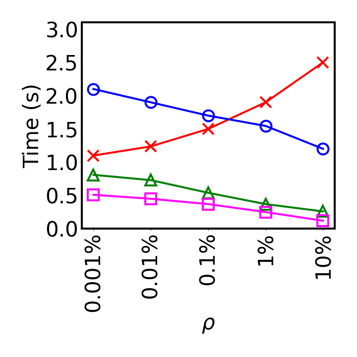
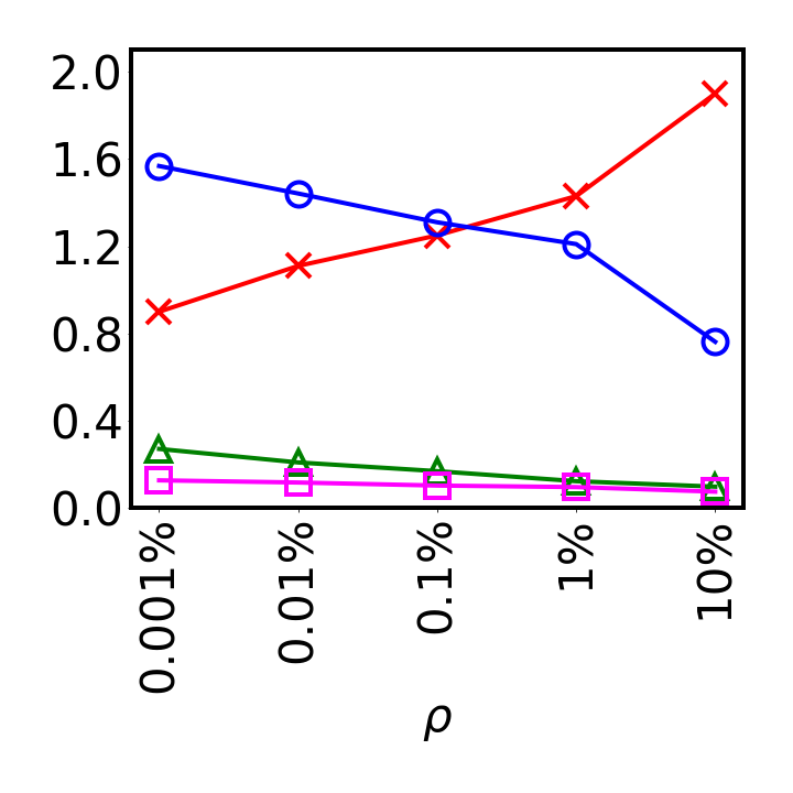
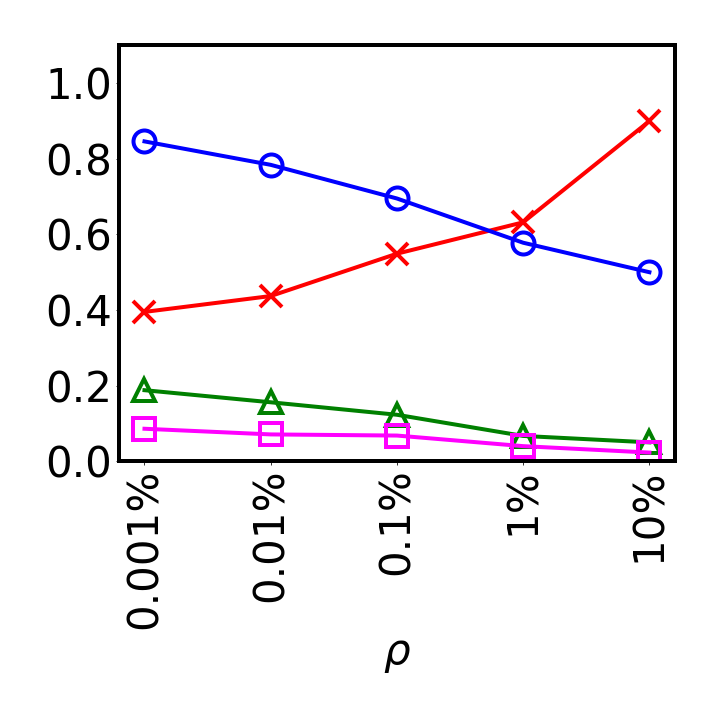
(j) CH	(k) PHL	(l) SF

Figure 9: Effect of varying $d_{c}$, $k$, $R_{ss}$ and $\rho$ for the three datasets

Datasets: We used real-world datasets of three cities that differ in terms of the road network size and crime statistics. Specifically, we extract the road network of Chicago, Philadelphia and San Francisco, using OpenStreetMap (OSM) and osm4routing parser in graph format (Table 2). All edge weights representing distances were scaled up and integer values were taken.

Edge $w_{ij}^{ss}$ Computation. We used crime datasets of Chicago (2001-2019), Philadelphia (2006-2019) and San Francisco (2003-2018) to assign weights ($w_{ij}^{ss}$) representing realistic ESSs of the respective road network graphs. We generated the ESSs of edges separately for three different ESS ranges $[1,s^{max}]$ denoted as $R_{ss}$ (see Table 3). The crime datasets include locations (latitude and longitude) of the crime incidents like robbery, motor vehicle theft, sexual offense, weapons violation, burglary and criminal damage to vehicle. For each edge, we count the number of crime incidents within $1$km and set it as the crime count of the edge. These crime counts are normalized to integers between the range $[1,s^{max}]$ representing crime scores. The crime score of each edge is converted to a safety score as $s^{max}+1-crimescore$, e.g., if $s^{max}$ is $10$ and the crime score for an edge is $10$, the safety score of the edge is $1$. The PSS of a path is computed based on the ESSs included in the path (Definition 2) and can be a float value.

Table 2: Road Network Dataset

Dataset	# Vertices	# Edges
Chicago (CH)	125,344	200,110
Philadelphia (PHL)	80,558	120, 581
San Francisco (SF)	40,528	72,819

Parameters: The parameter $d_{c}$ is a user specified parameter. Our solution works for any value of $d_{c}$. However, in experiments, we set $d_{c}$ to a value that is large enough to find the $k$SNNs for each query. Specifically, we define $d_{c}$ to be $\delta\times d^{k}$ where $d^{k}$ is the distance between $v_{l}$ and its $k^{th}$ closest POI and $\delta>1$ is a parameter in the experiments. Existing studies involving other parameterized queries also adapt similar settings to ensure query results are not empty ChenCJW13 and contain at least $k$ POIs shao2020efficiently .

We evaluate the algorithms by varying $\delta$, ESS range ($R_{ss}$), $k$, and the density of POIs ($\rho$), where density is the total number of POIs divided by the total number of vertices in the graph. The range and default values of the parameters are shown in Table 3. Similar to existing works ZhongLTZG15 ; abeywickrama2016k , we vary $k$ from 1 to 50 and set default value as 10. $R_{ss}$ is varied in the range of [1-5], [1-10] and [1-15]. Note that a smaller range (e.g., [1-2]) cannot effectively distinguish the safety variation of the road segments, whereas for a larger range (e.g., [1-30]), roads with a very small safety variation may have different PSSs and result in an increase in the length of the safest path. As shown in existing work abeywickrama2016k , most of the real world POIs have pretty low density. Therefore, we evaluate the algorithms by varying $\rho$ from $0.001\%$ to $10\%$ Following ZhongLTZG15 ; abeywickrama2016k , we set the default value of $\rho$ as 1%.

Table 3: Experiment Parameters

Parameters	Range	Default
$k$	1, 5, 10, 25, 50	10
$\delta$	1.25, 1.5, 1.75, 2	2
$R_{ss}$	1-5, 1-10, 1-15	1-10
$\rho$	0.001%, 0.01%, 0.1%, 1%, 10%	1%

Measures: For each experiment, we randomly select 100 vertices as query locations and report the average processing time to evaluate a $k$SNN query. We measure the preprocessing and storage cost for $Ct$-tree and SNVD in terms of the construction time, index size and the percentage of border vertices. All algorithms are implemented in C++ and the experiments are run on a 64-bit Windows 7 machine with an Intel Core i3-2350M, 2.30GHz processor and 4GB RAM.

7.1 Query Performance

Effect of $\delta$: Figures 9(a)–9(c) show that our algorithms can find $k$SNNs in real time. The query processing time slowly increases with the increase of $\delta$ (and consequently $d_{c}$) because more paths need to be explored for larger $\delta$. For $Ct$-tree-$k$SNN and SNVD-$k$SNN, we observe on average 11.6 times and 13.8 times faster processing time than that of R-tree-$k$SNN and on average 9.7 times and 12.7 times faster processing time than that of INE-$k$SNN, respectively.

Table 4: Pruning effectiveness in terms of the query processing time, number of network vertices accessed $\mid V_{a}\mid$ and number of valid paths explored by the algorithms. The Basic Algorithm in each approach only considers valid paths (i.e., only applies Pruning Rule 1). Each $\%$ value $x$ shown in a parenthesis indicates that the value in this cell is $x\%$ of the value of the Basic Algorithm of the same approach.

		CH			PHL			SF
	Setting	Time (ms)	$\mid V_{a}\mid$	# of Valid Paths	Time (ms)	$\mid V_{a}\mid$	# of Valid Paths	Time (ms)	$\mid V_{a}\mid$	# of Valid Paths
	Basic Algorithm	2225	2708	18223	755	2438	15867	1140	1905	12232
INE	Pruning Rule 2	1787 (80.31%)	2545 (93.9%)	14534 (79.75%)	581 (76.95%)	1831 (75.1%)	12783 (80.71%)	887 (77.8%)	1701 (77.5%)	8536 (69.78 % )
	Basic Algorithm	682	1601	4531	204	732	3673	109	351	2321
	Pruning Rule 2	485 (71.11%)	1056 (65.95%)	3287 (72.65%)	192 (94.11%)	601 (82.1%)	3328 (90.62%)	84 (82.35% )	318 (90.59%)	1881 (81.04%)
	Pruning Rule 3	460 (67.44%)	942 (58.83%)	2721 (60.05%)	194 (95.09%)	606 (82.7% )	3451 (93.97%)	81 (79.41 % )	302 (86.03%)	1745 (75.18% )
	Pruning Rule 4	471 (69.06%)	955 (59.65%)	2913 (64.31 % )	188 (92.15%)	588 (80.32%)	3198 (87.06%)	86 (81.13%)	315 (89.74%)	1801 (77.59%)
$Ct$-tree	All Pruning	377 (55.27%)	875 (54.65 % )	2621 (57.84%)	131 (64.8%)	523 (71.72%)	2665 (72.48%)	70 (68.62%)	281 (80.05%)	1535 (66.13%)
	Basic Algorithm	442	391	942	145	281	625	102	194	732
	Pruning Rule 2	349 (78.95%)	341 (87.21%)	699 (74.20% )	120 (82.75%)	249 (88.61%)	538 (86.08%)	78 (75.68%)	150 (77.31%)	627 (85.65%)
	Pruning Rules 5, 6	364 (82.35%)	356 (91.04%)	719 (76.32 % )	126 (84.13%)	255 (90.74%)	569 (91.04%)	81 (79.28%)	155 (79.89%)	639 (87.29%)
	Pruning Rule 7	379 (85.74%)	371 (94.88%)	772 (81.95%)	122 (84.13%)	205 (72.95%)	485 (77.6%)	71 (69.37%)	151 (77.84%)	643 (87.84%)
SNVD	All Pruning	229 (51.81%)	162 (58.56%)	623 (66.13%)	96 (66.21%)	165 (58.71%)	401 (64.16%)	53 (51.96%))	93 (47.94%)	409 (55.87%)

Effect of $k$: Figures 9(d)–9(f) show that the time increases with the increase of $k$, which is expected. The increase rate is low for $Ct$-tree-$k$SNN and SNVD-$k$SNN and shows almost a linear growth for varying $k$ from 1 to 50, whereas in case of INE-$k$SNN and R-tree-$k$SNN, the time increases significantly.

Effect of $R_{ss}$: Figures 9(g)–9(i) show that the time increases for R-tree-$k$SNN, INE-$k$SNN and $Ct$-tree-$k$SNN for larger $R_{ss}$, whereas for SNVD-$k$SNN the required time is the least among four algorithms and remains almost constant for all $R_{ss}$s. A larger $R_{ss}$ increases the height of the $Ct$-tree which in turn increases the number of subgraphs accessed by $Ct$-tree-$k$SNN. On the other hand, the number of subgraphs represented by SNVD cells does not vary with different $R_{ss}$s.

Effect of $\rho$: Figures 9(j)–9(l) show that the time decreases for INE-$k$SNN, Ct-$k$SNN and SNVD-$k$SNN with the increase of the POI density, $\rho$, whereas the time sharply increases for R-tree-$k$SNN. For INE-$k$SNN, a larger $\rho$ increases the possibility of finding the required POIs with less amount of incremental network expansion. For $Ct$-tree-$k$SNN, a larger $\rho$ increases the number of POIs in a $Ct$-tree node which in turn decreases the need of search in a larger subgraph. For SNVD-$k$SNN, the decrease curve is less steeper, since in SNVD-$k$SNN, the search time mainly depends on the number of SNVD cells that need to be explored rather than the total number of SNVD cells in the SNVD. On the other hand, for R-tree-$k$SNN, the number of candidates for $k$SNNs increases with the increase in $\rho$, which also causes increase in the number of independent safest path computations.

Effect of Datasets and Performance Scalability: In our experiments, we used three datasets that vary in the number of road network vertices, edges, POIs and crime distributions. Irrespective of the datasets, both $Ct$-tree-$k$SNN and SNVD-$k$SNN outperform R-tree-$k$SNN and INE-$k$SNN with a large margin. In addition, the query processing time linearly increases with increase of the dataset size in terms of the number of road network vertices, edges and POIs. Thus, our algorithms are scalable and applicable for all settings. In default parameter setting, the average time for Ct-kSNN is 371 ms, 123 ms and 66 ms for CH, PHL, and SF datasets, respectively. The average time for SNVD-kSNN is 223 ms, 96 ms and 41 ms for for CH, PHL, and SF datasets, respectively.

Pruning Effectiveness: In this set of experiments, we investigate the effectiveness of our pruning rules for the search space refinement. Table 4 summarizes the experiment results in the default setting of the parameters in terms of the query processing time, number of network vertices accessed $\|V_{a}\|$ and number of valid paths explored in road networks for different approaches when different pruning rules are applied. The Basic Algorithm includes only Pruning Rule 1(i.e., considers only valid paths). The performance of our algorithms are the best when all pruning rules are applied, which in turn means that each of the pruning rule contributes in improving the efficiency of our algorithms. Table 4 also shows why SNVD outperforms the other two algorithms. Note that the number of valid paths explored by the Basic Algorithm corresponds to $n_{p}$, $n^{\prime}_{p}$ and $n^{\prime\prime}_{p}$ in the complexity analyses of INE, $Ct$-tree and SNVD, respectively. Applying all pruning rules reduces the number of paths explored. The percentage values w.r.t. the Basic Algorithm are shown in parentheses. These percentage values can be used to obtain effect factors $r$, $r^{\prime}$ and $r^{\prime\prime}$ in the complexity analyses (e.g., $50\%$ reduction in number of paths implies that the effect factor is $100/50=2$). Generally, $n^{\prime\prime}_{p}>n^{\prime}_{p}>n_{p}$ and $r^{\prime\prime}>r^{\prime}>r$ which explains why SNVD is faster than $Ct$-tree and $Ct$-tree is faster than INE based approach.

Table 5: For $k=10$, comparison of $k$NN and $k$SNN queries including: average # of common POIs in $k$NNs and $k$SNNs; probability that $1$SNN is one of the POIs in $k$NNs; average PSS of the $k$ paths returned by $k$NN queries vs $k$SNN queries, and their ratios (i.e., $k$NN:$k$SNN); and average length of the $k$ paths returned by $k$NN vs $k$SNN queries, and their ratios.

		CH				PHL				SF
Measure		$\delta$=1.25	$\delta$ =1.5	$\delta$ = 1.75	$\delta$ = 2	$\delta$=1.25	$\delta$=1.5	$\delta$ = 1.75	$\delta$ = 2	$\delta$=1.25	$\delta$ =1.5	$\delta$ = 1.75	$\delta$ = 2
#common POIs		4.71	4.12	2.23	1.34	5.43	4.35	4.12	2.15	4.33	3.71	3.32	1.45
probability of $1$SNN in $k$NN		0.19	0.15	0.13	0.12	0.21	0.18	0.14	0.10	0.18	0.15	0.13	0.11
PSS	$k$NN	0.00029	0.00029	0.00029	0.00029	0.000035	0.000035	0.000035	0.000035	0.0004	0.0004	0.0004	0.0004
	$k$SNN	0.00091	0.0018	0.0024	0.0048	0.00006	0.00014	0.00045	0.00076	0.00055	0.00093	0.0012	0.003
ratio	1:3.1	1:6.2	1:8.3	1:16.5	1:1.7	1:4	1:12.8	1:21.7	1:1.4	1:2.3	1:3	1:7.6
Length	$k$NN	1311	1311	1311	1311	1222	1222	1222	1222	2446	2446	2446	2446
	$k$SNN	1507	1717	1941	2084	1504	1650	1882	2150	2960	3302	3717	3791
ratio	1:1.15	1:1.3	1:1.5	1:1.6	1:1.23	1:1.35	1:1.54	1:1.76	1:1.21	1:1.35	1:1.52	1:1.55

7.2 Query Effectiveness

We compare $k$SNNs with traditional $k$ nearest neighbors ($k$NNs) using default settings but varying $\delta$. Specifically, for each data set, we generate 100 query locations and run a kNN query and a kSNN query for each of these query locations, and report average results. We compare $k$SNNs with traditional $k$ nearest neighbors ($k$NNs) using default settings but varying $\delta$. Specifically, for each data set, we generate 100 query locations and run a kNN query and a kSNN query for each of these query locations, and report average results. Table 5 shows that $k$SNNs are significantly different from $k$NNs (see number of common POIs). Furthermore, the traditional $k$NN queries are not likely to include a POI that is also the first SNN. Finally, although the path lengths to $k$SNNs are longer, these paths are much safer. Specifically, the paths to $k$SNNs are up to $1.76$ times longer on average but they are up to $21$ times safer than the paths to $k$NNs. We also observe that the number of common POIs among $k$SNNs and $k$NNs decreases and the safety (PSS) of the paths from $v_{l}$ to $k$SNNs increases with the increase of $\delta$. Thus, in real-world scenarios where safety may be important for users, an application may show some $k$SNNs as well as some $k$NNs to give users more options to choose from.

7.3 Preprocessing and Storage

Query parameters $d_{c}$ and $k$ do not affect preprocessing and storage costs of the $Ct$-tree and SNVD. We show the effect of $R_{ss}$, $\rho$ and datasets on the preprocessing and storage costs of the $Ct$-tree and SNVD in experiments.

$Ct$-tree: Figure 10 shows that the $Ct$-tree construction time, index size and the percentage of border vertices slowly increase with the increase of $R_{ss}$ and dataset size. The effect of dataset size on the increasing trend is expected, whereas the reason behind the increase of processing time and storage for $R_{ss}$ is that the height of a $Ct$-tree increases with the increase of $R_{ss}$. The $Ct$-tree stores 1% to 5% of the total number of vertices in the road network as border vertices, which is negligible. We observed that the density of POIs $\rho$ does not affect construction cost as the construction of $Ct$-tree does not depend on the number of POIs but mainly on the ESS values of the edges. While border to POI distances need to be maintained, the effect on index size is not significant.

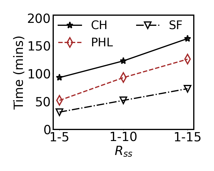
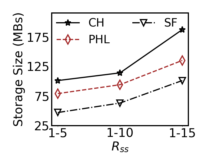
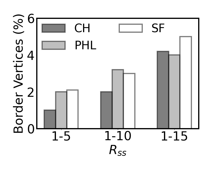
(a)	(b)	(c)

Figure 10: Ct-tree: Effect of $R_{ss}$ and datasets on (a) construction time (b) storage size and (c) % of border vertices

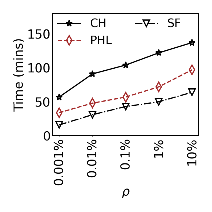
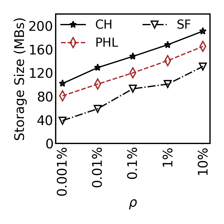
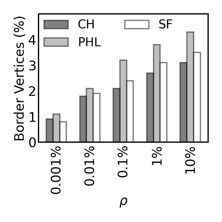
(a)	(b)	(c)

Figure 11: SNVD: Effect of $\rho$ and datasets on (a) construction time (b) storage size and (c) % of border vertices

SNVD: The storage size of an SNVD includes SNVD cell information and distance information. We observe no significant variation in the construction time, storage size and the number of border vertices for different ESS ranges $R_{ss}$. The number of Voronoi cells in an SNVD is equal to the number of POIs and thus, the construction time, storage size and the number of border vertices increase with the increase of $\rho$ and the dataset size (Figure 11). The percentage of border vertices for all datasets is less than 5% of the total number of vertices in the road network, which is negligible.

$Ct$-tree vs. SNVD: The construction times for $Ct$-tree and SNVD are comparable whereas SNVD is up to 1.6 times bigger in size than $Ct$-tree. Specifically, for default settings (i.e., $R_{ss}=1-10$, $\rho=1\%$), the construction time for $Ct$-tree for the three datasets ranges from $54-123$ minutes as compared to $50-122$ minutes for SNVD. On the other hand, the index size of $Ct$-tree for the three datasets ranges from $63-114$ MB compared to $101-168$ MB for SNVD.

8 Conclusions and Future Work

In this paper, we introduced $k$ Safest Nearby neighbor ($k$SNN) queries in road networks and formulated the measure of path safety score. We proposed novel indexing structures, $Ct$-tree and a safety score based Voronoi diagram (SNVD), to efficiently evaluate $k$SNN queries. We adapt the INE based technique and the $R$-tree based technique to develop two baselines to find $k$SNNs. Our extensive experimental study on three real-world datasets shows that $Ct$-tree and SNVD based approaches are up to an order of magnitude faster than the baselines. Comparing $Ct$-tree and SNVD on default settings, both approaches have comparable construction time whereas SNVD index is around 1.6 times bigger than $Ct$-tree but is 1.2-1.7 times faster in terms of query processing cost. Thus, if the storage is not an issue, one should go for the SNVD based approach to get faster query processing performance.

An interesting direction for future work is to investigate skyline routes GalbrunPT16 ; josse2015tourismo considering multiple criteria such as distance, safety, travel time etc. Here, the safety itself may consist of multiple attributes corresponding to different crime types and inconveniences, e.g., robbery, harassment, bumpy road etc.

Acknowledgments. Tanzima Hashem is supported by basic research grant of Bangladesh University of Engineering and Technology. Muhammad Aamir Cheema is supported by the Australian Research Council (ARC) FT180100140 and DP180103411.

Appendix

Appendix A Proof of Lemma 1

Proof

From Definition 2, $pss(pt_{lj})=\frac{1}{\sum_{s=1}^{s^{max}}{w_{s}\times pt_{lj}.d_{s}}}$. Replacing $pt_{lj}.d_{s}$ according to Definition 1, we have

$$pss(pt_{lj})=\frac{1}{\sum_{s=1}^{s^{max}}{w_{s}\times\sum_{e_{xy}\in pt_{lj}\wedge w_{xy}^{ss}=s}w^{d}_{xy}}}$$

$$=\frac{1}{\sum_{s=1}^{s^{max}}{w_{s}\times(\sum_{e_{xy}\in pt_{li}\wedge w_{xy}^{ss}=s}w^{d}_{xy}+\sum_{e_{xy}\in pt_{ij}\wedge w_{xy}^{ss}=s}w^{d}_{xy}})}$$

$$=\frac{1}{\sum_{s=1}^{s^{max}}{(w_{s}\times\sum_{e_{xy}\in pt_{li}\wedge w_{xy}^{ss}=s}w^{d}_{xy}})+(w_{s}\times\sum_{e_{xy}\in pt_{ij}\wedge w_{xy}^{ss}=s}w^{d}_{xy})}$$

$$=\frac{1}{(\sum_{s=1}^{s^{max}}{w_{s}\times pt_{li}.d_{s}})+(\sum_{s=1}^{s^{max}}{w_{s}\times pt_{ij}.d_{s}})}$$

$$=\frac{1}{\frac{1}{pss(pt_{li})}+\frac{1}{pss(pt_{ij})}}$$

∎

Appendix B Proof of Lemma 2

Proof

It is straightforward to show that $pt^{\prime}_{lj}\oplus pt_{jk}$ is at least as short as $pt_{lj}\oplus pt_{jk}$ because $pt^{\prime}_{lj}$ is at least as short as $pt_{lj}$ and $pt_{jk}$ is same in both paths. According to Lemma 1, the PSS of $pt^{\prime}_{lj}\oplus pt_{jk}$ is $\frac{1}{\frac{1}{pss(pt^{\prime}_{lj})}+\frac{1}{pss(pt_{ik})}}$ and the PSS of $pt_{lj}\oplus pt_{jk}$ is $\frac{1}{\frac{1}{pss(pt_{lj})}+\frac{1}{pss(pt_{ik})}}$. $\frac{1}{pss(pt_{ik})}$ part is same in the PSS of both paths. Since $pss(pt^{\prime}_{lj})\geq pss(pt_{lj})$, $\frac{1}{\frac{1}{pss(pt^{\prime}_{lj})}+\frac{1}{pss(pt_{ik})}}\geq\frac{1}{\frac{1}{pss(pt_{lj})}+\frac{1}{pss(pt_{ik})}}$. Thus, $pt^{\prime}_{lj}\oplus pt_{jk}$ is at least as safe as $pt_{lj}\oplus pt_{jk}$. ∎

References

- [1] Tenindra Abeywickrama, Muhammad Aamir Cheema, and David Taniar. k-nearest neighbors on road networks: A journey in experimentation and in-memory implementation. Proc. VLDB Endow., 2016.
- [2] Saad Aljubayrin, Jianzhong Qi, Christian S. Jensen, Rui Zhang, Zhen He, and Yuan Li. Finding lowest-cost paths in settings with safe and preferred zones. The VLDB Journal, 26(3):373–397, 2017.
- [3] Saad Aljubayrin, Jianzhong Qi, Christian S. Jensen, Rui Zhang, Zhen He, and Zeyi Wen. The safest path via safe zones. In ICDE, pages 531–542, 2015.
- [4] Anika Anwar and Tanzima Hashem. Optimal obstructed sequenced route queries in spatial databases, 2017.
- [5] BBC. Street harassment ’relentless’ for women and girls, 23 October 2018.
- [6] Norbert Beckmann, Hans-Peter Kriegel, Ralf Schneider, and Bernhard Seeger. The r*-tree: An efficient and robust access method for points and rectangles. SIGMOD Rec., 19(2):322–331, May 1990.
- [7] Spencer Chainey and Jerry Ratcliffe. GIS and crime mapping. John Wiley & Sons, 2013.
- [8] Muhammad Aamir Cheema. Indoor location-based services: challenges and opportunities. SIGSPATIAL Special, 10(2):10–17, 2018.
- [9] Lisi Chen, Gao Cong, Christian S. Jensen, and Dingming Wu. Spatial keyword query processing: An experimental evaluation. Proc. VLDB Endow., 6(3):217–228, 2013.
- [10] Edsger W. Dijkstra. A note on two problems in connexion with graphs. Numerische Mathematik, 1:269–271, 1959.
- [11] Martin Erwig. The graph voronoi diagram with applications. Networks, 36(3):156–163, 2000.
- [12] Raphael A. Finkel and Jon Louis Bentley. Quad trees: A data structure for retrieval on composite keys. Acta Inf., 4:1–9, 1974.
- [13] Kaiqun Fu, Yen-Cheng Lu, and Chang-Tien Lu. TREADS: a safe route recommender using social media mining and text summarization. In SIGSPATIAL, pages 557–560, 2014.
- [14] Esther Galbrun, Konstantinos Pelechrinis, and Evimaria Terzi. Urban navigation beyond shortest route: The case of safe paths. Inf. Syst., 2016.
- [15] Robert Geisberger, Peter Sanders, Dominik Schultes, and Daniel Delling. Contraction hierarchies: Faster and simpler hierarchical routing in road networks. In WEA, pages 319–333, 2008.
- [16] Antonin Guttman. R-trees: A dynamic index structure for spatial searching. In SIGMOD, page 47–57, 1984.
- [17] Tanzima Hashem, Tahrima Hashem, Mohammed Eunus Ali, and Lars Kulik. Group trip planning queries in spatial databases. In SSTD, 2013.
- [18] Gísli R. Hjaltason and Hanan Samet. Distance browsing in spatial databases. ACM Trans. Database Syst., 1999.
- [19] Plan International. 1 in 5 girls have experienced street harassment during lockdown, 20 April 2020.
- [20] Fariha Tabassum Islam, Tanzima Hashem, and Rifat Shahriyar. A privacy-enhanced and personalized safe route planner with crowdsourced data and computation. In ICDE, pages 229–240, 2021.
- [21] Gregor Jossé, Klaus Arthur Schmid, Andreas Züfle, Georgios Skoumas, Matthias Schubert, and Dieter Pfoser. Tourismo: A user-preference tourist trip search engine. In SSTD, pages 514–519, 2015.
- [22] Jaewoo Kim, Meeyoung Cha, and Thomas Sandholm. Socroutes: safe routes based on tweet sentiments. In WWW, pages 179–182, 2014.
- [23] Mohammad R. Kolahdouzan and Cyrus Shahabi. Voronoi-based K nearest neighbor search for spatial network databases. In VLDB, 2004.
- [24] Alain Lambert and Dominique Gruyer. Safe path planning in an uncertain-configuration space. In ICRA, pages 4185–4190, 2003.
- [25] Ken C. K. Lee, Wang-Chien Lee, Baihua Zheng, and Yuan Tian. ROAD: A new spatial object search framework for road networks. IEEE TKDE, 2012.
- [26] Louise Leenen, Alexander Terlunen, and Herman Le Roux. A constraint programming solution for the military unit path finding problem. In Mobile Intelligent Autonomous Systems, pages 225––240. 2012.
- [27] Lingxiao Li, Muhammad Aamir Cheema, Mohammed Eunus Ali, Hua Lu, and David Taniar. Continuously monitoring alternative shortest paths on road networks. Proc. VLDB Endow., 13(12):2243–2255, 2020.
- [28] Lingxiao Li, Muhammad Aamir Cheema, Hua Lu, Mohammed Eunus Ali, and Adel N Toosi. Comparing alternative route planning techniques: A comparative user study on melbourne, dhaka and copenhagen road networks. IEEE Trans. Knowl. Data Eng., 2021.
- [29] Zijian Li, Lei Chen, and Yue Wang. G*-tree: An efficient spatial index on road networks. In ICDE, pages 268–279, 2019.
- [30] Tiantian Liu, Huan Li, Hua Lu, Muhammad Aamir Cheema, and Lidan Shou. Towards crowd-aware indoor path planning. Proc. VLDB Endow., 2021.
- [31] Saeed Nadi and Mahmood Reza Delavar. Multi-criteria, personalized route planning using quantifier-guided ordered weighted averaging operators. Int. J. Appl. Earth Obs. Geoinformation, 2011.
- [32] Mangai Natarajan. Crime in developing countries: the contribution of crime science, 2016.
- [33] Atsuyuki Okabe, Barry Boots, Kokichi Sugihara, Sung Nok Chiu, and D. G. Kendall. Spatial Tessellations: Concepts and Applications of Voronoi Diagrams, Second Edition. Wiley, 2000.
- [34] Atsuyuki Okabe, Toshiaki Satoh, Takehiro Furuta, Atsuo Suzuki, and K. Okano. Generalized network voronoi diagrams: Concepts, computational methods, and applications. IJGIS, 22(9):965–994, 2008.
- [35] Dimitris Papadias, Jun Zhang, Nikos Mamoulis, and Yufei Tao. Query processing in spatial network databases. In VLDB, pages 802–813, 2003.
- [36] Maytham Safar, Dariush Ebrahimi, and David Taniar. Voronoi-based reverse nearest neighbor query processing on spatial networks. Multimedia Syst., 15(5):295–308, 2009.
- [37] Chaluka Salgado, Muhammad Aamir Cheema, and David Taniar. An efficient approximation algorithm for multi-criteria indoor route planning queries. In SIGSPATIAL, pages 448–451, 2018.
- [38] Hanan Samet, Jagan Sankaranarayanan, and Houman Alborzi. Scalable network distance browsing in spatial databases. In SIGMOD, pages 43–54, 2008.
- [39] Jagan Sankaranarayanan, Houman Alborzi, and Hanan Samet. Efficient query processing on spatial networks. In International Workshop on GIS, pages 200–209, 2005.
- [40] Sumit Shah, Fenye Bao, Chang-Tien Lu, and Ing-Ray Chen. CROWDSAFE: crowd sourcing of crime incidents and safe routing on mobile devices. In SIGSPATIAL, pages 521–524, 2011.
- [41] Zhou Shao, Muhammad Aamir Cheema, David Taniar, Hua Lu, and Shiyu Yang. Efficiently processing spatial and keyword queries in indoor venues. IEEE Trans. Knowl. Data Eng., 2020.
- [42] Mehdi Sharifzadeh, Mohammad R. Kolahdouzan, and Cyrus Shahabi. The optimal sequenced route query. The VLDB Journal, 2008.
- [43] Bojie Shen, Muhammad Aamir Cheema, Daniel Harabor, and Peter J Stuckey. Euclidean pathfinding with compressed path databases. In IJCAI, 2020.
- [44] Bojie Shen, Muhammad Aamir Cheema, Daniel D Harabor, and Peter J Stuckey. Fast optimal and bounded suboptimal euclidean pathfinding. Artificial Intelligence, 302:103624, 2022.
- [45] Mukund Pratap Singh, Pitam Singh, and Priyamvada Singh. Fuzzy ahp-based multi-criteria decision-making analysis for route alignment planning using geographic information system (GIS). J. Geogr. Syst., 2019.
- [46] Valerie Spicer, Justin Song, Patricia Brantingham, Andrew Park, and Martin A Andresen. Street profile analysis: A new method for mapping crime on major roadways. Applied Geography, 69:65–74, 2016.
- [47] Christopher H Stubbert, Stephen F Pires, and Rob T Guerette. Crime science and crime epidemics in developing countries: a reflection on kidnapping for ransom in colombia, south america. Crime Science, 4(1):23, 2015.
- [48] Jur P. van den Berg and Mark H. Overmars. Planning the shortest safe path amidst unpredictably moving obstacles. In Algorithmic Foundation of Robotics VII, pages 103–118, 2006.
- [49] Kefeng Xuan, Geng Zhao, David Taniar, Bala Srinivasan, Maytham Safar, and Marina L. Gavrilova. Network voronoi diagram based range search. In AINA, pages 741–748, 2009.
- [50] Ruicheng Zhong, Guoliang Li, Kian-Lee Tan, Lizhu Zhou, and Zhiguo Gong. G-tree: An efficient and scalable index for spatial search on road networks. IEEE TKDE, 27(8):2175–2189, 2015.