The growth and distribution of large circles on translation surfaces

Abstract

We consider circles on a translation surface $X$, consisting of points joined to a common center point by a geodesic of length $R$. We show that as $R\to\infty$ these circles distribute to a measure on $X$ which is equivalent to the area. In the last section we consider analogous results for closed geodesics.

1 Introduction

Given a closed Riemannian surface of constant curvature and genus $g\geq 2$, several authors have considered circles consisting of those points which are joined by geodesics of a common length (which can be thought of as radii) to a common point (which can be viewed as the center). Equivalently, we can consider the projections of circles from its universal cover. As the radius tends to infinity, these circles become equidistributed with respect to Haar measure. In the case $g=1$ this is an easy exercise and for $g\geq 2$ this was shown by Randol [18].

We want to consider the natural generalization to translation surfaces $X$. More precisely, given a point $x\in X$ and $R>0$, we can naturally associate a one dimensional curve $\mathcal{C}(x,R)\subset X$ consisting of those points on $X$ joined to $x$ by a geodesic of length $R$. On $X$ the radial geodesics are either straight line segments or concatenations of straight line segments and saddle connections joining singularities. Let $\ell(\mathcal{C}(x,R))$ denote the total length of the one dimensional curve $\mathcal{C}(x,R)$. Despite the surface being flat (except at the finite set of singularities $\Sigma$), the length of $\mathcal{C}(x,R)$ actually grows exponentially in $R$ because of how geodesics behave at the singularities. In particular, we have that

$$h(X):=\lim_{R\to\infty}\frac{1}{R}\log\ell(\mathcal{C}(x,R))$$

exists and is positive. We will call $h(X)$ the entropy of the surface. In his PhD thesis, Dankwart [4] originally defined (volume) entropy in terms of orbital counting. In [3], we defined a notion of entropy in terms of the rate of growth of the volume of a ball in the universal cover, by analogy with the definition due to Manning for Riemannian manifolds [11]. More precisely, let $\widetilde{X}$ be the universal cover for $X$ and let $\mathcal{B}(\widetilde{x},R)$ be a ball in $\widetilde{X}$ of radius $R>0$ centered at $\widetilde{x}$. If we then write $\hbox{\rm Vol}_{\widetilde{X}}(\mathcal{B}(\widetilde{x},R))$ for the volume of the ball, then the original definition of (volume) entropy is

$$h(X)=\lim_{R\to\infty}\frac{1}{R}\log\hbox{\rm Vol}_{\widetilde{X}}(B(\widetilde{x},R)).$$

However, these different definitions are easily seen to be equivalent. The definition (1.1) in terms of the length $\ell(\mathcal{C}(x,R))$ has the slight conceptual advantage that it does not necessitate going to the universal cover since the length of the curve $\mathcal{C}(x,R)$ has a natural interpretation on $X$.

Our first main result improves on (1.1) by giving the natural asymptotic formula for the length of the curve.

Theorem A (Asymptotic length formula).

There exists $C=C(x)>0$ such that

$$\ell(\mathcal{C}(x,R))\sim Ce^{h(X)R}\hbox{ as }R\to\infty\quad\left(\hbox{i.e.,}\lim_{R\to\infty}\frac{\ell(\mathcal{C}(x,R))}{Ce^{h(X)R}}=1\right).$$

The asymptotic formula in Theorem A is reminiscent of the simpler corresponding result for Riemannian surfaces of constant negative curvature (without singularities) of genus $g\geq 2$ which is easily deduced from [8]. See also work by Margulis [12].

Next we want to give a distributional result for the circles $\mathcal{C}(x,R)$. We define a family of natural probability measures $\mu_{R}$ supported on the sets $\mathcal{C}(x,R)$ for $R>0$. These correspond to the normalized arc length measure on the curve $\mathcal{C}(x,R)$.

Definition 1.1.

We can define a family of probability measures $\mu_{R}$ ($R>0$) on $X$ by

$$\mu_{R}(A)=\frac{\ell(\mathcal{C}(x,R)\cap A)}{\ell(\mathcal{C}(x,R))},\hbox{ for Borel sets $A\subset X$,}$$

where $\ell(\mathcal{C}(x,R)\cap A)$ denotes the one dimensional measure of $\mathcal{C}(x,R)\cap A$.

The next result describes the convergence of the probability measures $\mu_{R}$ as the radius $R$ tends to infinity.

Theorem B (Circle distribution result).

The sequence of measures $(\mu_{R})_{R>0}$ converge in the weak-star topology to a measure $\mu$ which is equivalent to the volume measure $\hbox{\rm Vol}_{X}$ on $X$, i.e. $\lim_{R\to\infty}\int fd\mu_{R}=\int fd\mu$ for any $f\in C(X)$.

We note that this is not quite a traditional equidistribution result in the sense that although $\mu$ is equivalent to the volume measure $\hbox{\rm Vol}_{X}$, the Radon-Nikodym derivative $d\mu/d\hbox{\rm Vol}_{X}$ is not constant.

Our method of proof for both theorems is based on an approach using complex functions and Tauberian theorems developed in [3].

In §2 we describe the basic definitions and examples. In §3 we present the basic approach to describing the growth of circles (and the proof of Theorem A). In §4 we use a similar method to prove a growth rate for weighted balls on the universal cover of $X$ and in §5 we use the results from §4 to deduce Theorem B. Finally in §6 we discuss analogous results to Theorem A and B for closed geodesics.

2 Translation surfaces and geodesics

In this section, we recall a convenient definition of translation surfaces and their basic properties. A good reference for this material (and more background) are the surveys [21] and [20]. We will use the same notation as in [3].

Roughly speaking, a translation surface $X$ is a closed surface endowed with a flat metric except at, possibly, a finite number of singular points such that there is a well defined notion of north at every non-singular point.

Singularities on translation surfaces are cone-points. To see what this means, consider the following construction: let $k\in\mathbb{N}$ and take $(k+1)$ copies of the upper half plane with the usual metric and $(k+1)$ copies of the lower half plane. Then glue them together along the half infinite rays $[0,\infty)$ and $(-\infty,0]$ in cyclic order (Figure 1).

Figure 1: Four half-disks of radius cyclic fashion. A cone point of angle $4\pi$ on a translation surface has a neighbourhood isometric to a neighbourhood of the the origin in the picture.

There are a few equivalent definitions which appear in the literature; however, we will present the one which is most suited to our needs.

Definition 2.1.

A translation surface is a closed topological surface $X$, together with a finite set of points $\Sigma$ and an atlas of charts to $\mathbb{C}$ on $X\backslash\Sigma$, whose transition maps are translations. Furthermore, we require that for each point $x\in\Sigma$, there exists some $k\in\mathbb{N}$ and a homeomorphism of a neighborhood of $x$ to a neighbourhood of the origin in the $2k+2$ half plane construction that is an isometry away from $x$.

It is easy to see that the above definition gives a locally Euclidean metric on $X\backslash\Sigma$. The set $\Sigma=\{x_{1},\ldots,x_{n}\}$ is the set of singularities or cone-points on the surface, where the singularity $x_{i}$ has a cone-angle of the form $2\pi(k(x_{i})+1)$ with $k(x_{i})\in\mathbb{N}$.

In the absence of singularities, the surface is a torus, but if $X$ has genus at least $2$ then by a simple consideration of the Gauss-Bonnet theorem we see that there must be at least one singularity. Henceforth, we will consider the case $\Sigma\neq\emptyset$.

We recall a simple construction for translation surfaces which is particularly useful in giving examples. Let $\mathbb{P}$ denote a polygon in the Euclidean plane $\mathbb{R}^{2}$ for which every side has an opposite side which is parallel and of the same length. By identifying these opposite sides we obtain a translation surface. The vertices may contribute to the singularities and the total angle (i.e., the cone-angle) around any singularity is $2\pi k$, where $k>1$.

A path which does not pass through singularities in its interior is a locally distance minimizing geodesic if it is a straight line segment. This includes geodesics which start and end at singularities, which are known as saddle connections. In particular, we will consider oriented saddle connections. Let

$${\mathcal{S}}=\{s_{1},s_{2},s_{3},...\}$$

denote the countably infinite family of oriented saddle connections on the translation surface ordered by non-decreasing length. We let $i(s),t(s)\in\Sigma$ denote the initial and terminal singularities, respectively, of the oriented saddle connection $s\in\mathcal{S}$.

A key difference to the Euclidean case is that geodesics (i.e., local distance minimizing curves) can change direction if they go through a singular point. A pair of line segments ending and beginning, respectively, at a singular point form a geodesic if the smallest angle between them is at least $\pi$. In particular, this leaves $2\pi k(x_{i})$ worth of angles for the geodesic to emerge from the singularity $x_{i}$. This happens because we are studying the growth of locally distance minimizing geodesics.

The following particular type of geodesic will play a key role in our later analysis.

Definition 2.2.

We can denote by $p=(s_{1},\ldots,s_{n})$ an (allowed) finite word of oriented saddle connections corresponding to a geodesic path, which we call saddle connection paths. We denote by $|p|=n$ the word length and by

$$\ell(p)=\sum_{i=1}^{n}\ell(s_{i})$$

the geometric length. We write $i(p)=i(s_{1})$ and $t(p)=t(s_{n})$.

Let $x\in\Sigma$ and define the set $\mathcal{P}(x,R)$ to be the set of saddle connection paths which start at $x$ and have length less than or equal to $R$. Let $\mathcal{P}(x)=\cup_{R>0}\mathcal{P}(x,R)$ denote the set of all such paths regardless of length.

We conclude this section with two simple examples of translation surfaces.

Example 2.3 (Slit surface).

We can consider two copies of the flat torus $\mathbb{T}^{2}=\mathbb{R}^{2}/\mathbb{Z}^{2}$ with a slit removed. In identifying the two surfaces along the slits one obtains a surface of genus $2$ with two singularities each with cone-angle $4\pi$ (coming from the ends of the slits). See Figure 2.

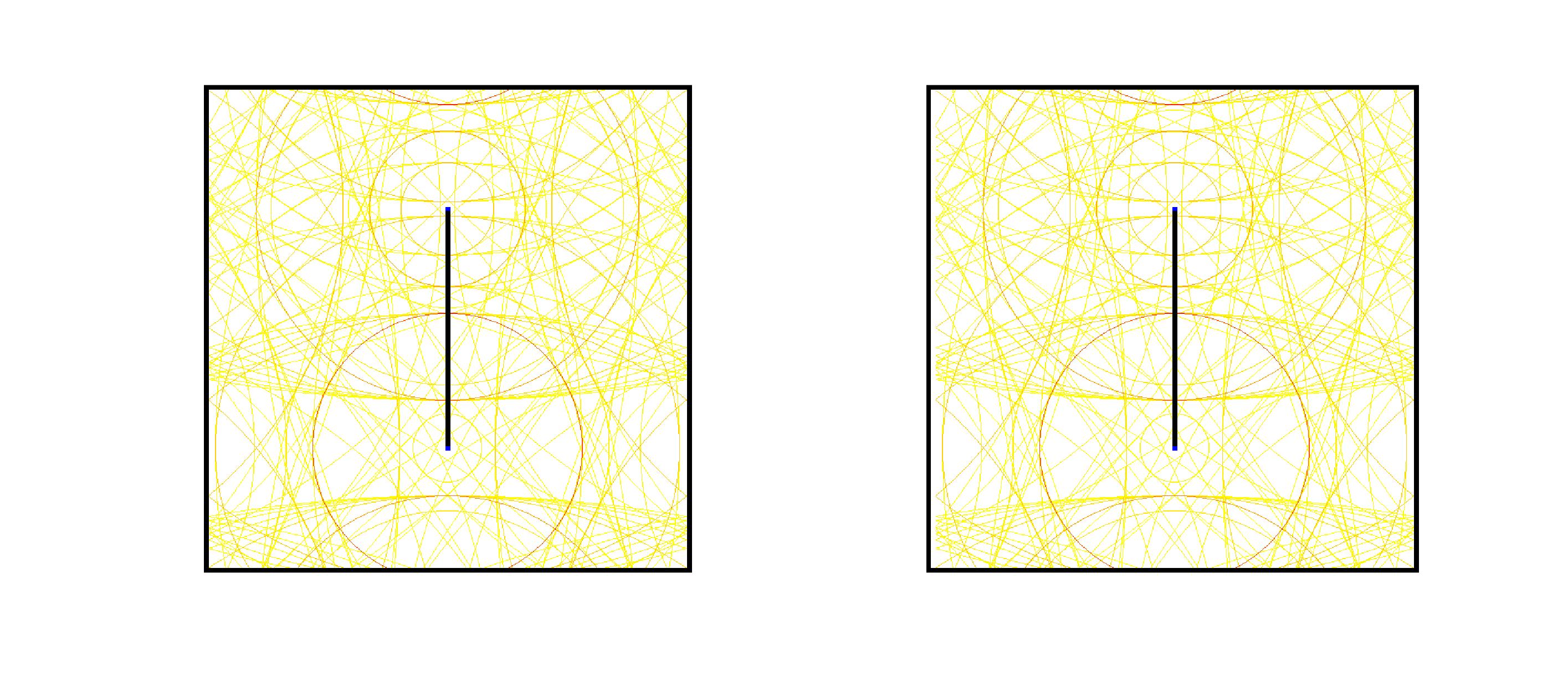
Figure 2: A circle of large radius projected onto a translation surface consisting of two slit tori

Example 2.4 ($L$-shaped surface).

We can consider an $L$-shaped polygon which is a square-tiled surface where the identification of opposite sides gives a surface of genus $2$ and only one singularity (see Figure 3). The singularity comes from the identification of the corners and has a cone-angle of $6\pi$.

Because this surface forms a ramified cover of the standard torus, we see that for each coprime pair $(m,n)\in\mathbb{Z}^{2}$, there are three saddle connections whose holonomy correspond to $(m,n)$. Furthermore, we can understand the saddle connection paths on this surface by noting that a saddle connection with holonomy $(m,n)$ can concatenate with any other saddle connection with the same holonomy or two of the three saddle connections with holonomy $(m^{\prime},n^{\prime})\neq(m,n)$.

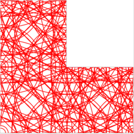
Figure 3: A large circle projected onto a $L$-shaped domain.

3 Proof of Theorem A

In this section, we provide a proof of Theorem A. This proof follows the strategy for the asymptotic for $\hbox{Vol}_{X}(\mathcal{B}(\widetilde{x},R))$ developed in [3]. From now on, fix a translation surface $X$, a singularity $x\in\Sigma$, and denote the entropy of $X$ by $h=h(X)$.

3.1 Large circles

We will first express the length $\ell(\mathcal{C}(x,R))$ of the curve $\mathcal{C}(x,R)$ using saddle connection paths. For convenience, we have assumed that $x$ is a singularity; however, a similar argument would work if we considered a general point on the surface instead.

The radii for the circles $\mathcal{C}(x,R)$ correspond to saddle connection paths $p=(s_{1},\ldots,s_{n})$ which start at $x$ and are followed by a final line segment of length $r\geq 0$, say, which begins at $t(p)$ and contains no other singularities. In particular, this geodesic will have length $\ell(s_{1})+\cdots+\ell(s_{n})+r$.

Lemma 3.1.

Let $x\in\Sigma$. Then for $R>0$

$$\ell(\mathcal{C}(x,R)) =2\pi(k(x)+1)R+\sum_{p\in\mathcal{P}(x,R)}2\pi k(t(p))\left(R-\ell(p)\right).$$

Proof.

The proof is immediate given that locally distance minimizing geodesics starting from a singularity are given by a saddle connection path $p=s_{1}s_{2}\ldots s_{n}$ with $\ell(s_{1})+\cdots+\ell(s_{n})\leq R$ followed by a straight line starting at the last singularity $t(p)$ of length $R-\ell(s_{1})+\cdots+\ell(s_{n})$. In particular, this last segment contributes to a Euclidean arc of length $2\pi k(t(p))(R-(\ell(s_{1})+\cdots+\ell(s_{n})))$. ∎

It is a simple observation (for example from (3.1)) that the length $\ell(C(x,R))$ is a monotone increasing function of $R>0$. This simple property is necessary for our method of proving the asymptotic formula in Theorem A.

3.2 Tauberian theorem and complex functions

The proof of Theorem A involves the application of the following classical Tauberian theorem to the monotone and continuous function $\ell(\mathcal{C}(x,R))$.

Theorem 3.2 (Ikehara–Wiener Tauberian theorem, cf. [5]).

Let $\rho:\mathbb{R}^{+}\to\mathbb{R}^{+}$ be a non-decreasing and right-continuous function. Formally denote $\eta(z):=\int_{0}^{\infty}e^{-zR}d\rho(R)$, for $z\in\mathbb{C}$. Assume that $\eta(z)$ has the following properties:

1. there exists some $a>0$ such that $\eta(z)$ is analytic on $Re(z)>a$;

2. $\eta(z)$ has a meromorphic extension to a neighbourhood of the half-plane $Re(z)\geq a$;

3. $a$ is a simple pole for $\eta(z)$, i.e., $C=\lim_{\epsilon\searrow 0}(z-a)\eta(z)$ exists and is positive; and

4. the extension of $\eta(z)$ has no poles on the line $Re(z)=a$ other than $a$.

Then $\rho(R)\sim\frac{C}{a}e^{aR}$ as $R\rightarrow\infty$.

Remark 3.3.

Theorem 3.2 is a reformulation of the standard Tauberian theorem for the case $a=1$.

In order to apply the above Tauberian theorem to $\ell(\mathcal{C}(x,R))$, we need to define and study the following complex function.

Definition 3.4.

Since $\ell(\mathcal{C}(x,R))$ is monotone increasing we can formally define the Riemann-Stieltjes integral

$$\eta(z)=\int_{0}^{\infty}e^{-zR}d\ell(\mathcal{C}(x,R))\hbox{ for }z\in\mathbb{C}.$$

Using (1.1), it is easy to see that the complex function $\eta(z)$ converges to an analytic function for $Re(z)>h$.

In order to show that $\eta(z)$ satisfies the properties required to apply the Tauberian theorem, we will first rewrite $\eta(z)$ in terms of certain infinite matrices which contain information about saddle connection paths on $X$ and their lengths. The following three properties of saddle connection paths on translation surfaces guarantee that the matrices have spectral properties which allow us to deduce that $\eta(z)$ has the required properties.

Lemma 3.5.

For all translation surfaces $X$, with corresponding oriented saddle connection set $\mathcal{S}$, the following statements hold.

1. For all $\sigma>0$ we have $\sum_{s\in\mathcal{S}}e^{-\sigma\ell(s)}<\infty$;

2. For any directed saddle connections $s,s^{\prime}\in\mathcal{S}$ there exists a saddle connection path $p$ beginning with $s$ and ending with $s^{\prime}$; and

3. There does not exist a $d>0$ such that

   $$\{\ell(c)\hbox{ : }c\hbox{ is a closed saddle connection path}\}\subset d\mathbb{N}.$$

These simple observations are taken from [3].

We now turn to expressing $\eta(z)$ in terms of infinite matrices in order to obtain the desired meromorphic extension of $\eta(z)$.

3.3 Infinite matrices

We will first show that $\eta(z)$ can be written in terms of saddle connection paths on $X$. We will then rewrite $\eta(z)$ in terms of countably infinite matrices which capture the saddle connection path data of $\mathcal{P}(x)$.

Lemma 3.6.

For $Re(z)>h$, we have that

$$\eta(z) =\frac{2\pi}{z}(k(x)+1)+\frac{2\pi}{z}k(t(p))\sum_{p\in\mathcal{P}(x)}e^{-z\ell(p)}.$$

Proof.

We begin with the contribution to $\ell(\mathcal{C}(x,R))$ that comes from the Euclidean circle of radius $R$ and cone-angle $2\pi(k(x)+1)$. This involves considering

$$2\pi(k(x)+1)\int_{0}^{\infty}e^{-zR}dR=-\frac{2\pi}{z}(k(x)+1)\left[e^{-zR}\right]_{0}^{\infty}=\frac{2\pi}{z}(k(x)+1).$$

We see from (3.1) that the Euclidean circles with cone-angle $2\pi k(t(p))$ centered at $t(p)$ following the saddle connection path $p=(s_{1},\ldots,s_{n})$ will have radius $R-\ell(p)$. The contribution to $\eta(z)$ from saddle connection path $p$ will be

$$2\pi k(t(p))\int_{\ell(p)}^{\infty}e^{-zR}d\left(R-\ell(p)\right) =2\pi k(t(p))e^{-z\ell(p)}\int_{0}^{\infty}e^{-zR}dR$$

$$=\frac{2\pi k(t(p))}{z}e^{-z\ell(p)}$$

by the change of variable $T=R-\ell(p)$. By (1.1) we have that the summation over all of these contributions is uniformly convergent for $Re(z)>h$. This gives the required result. ∎

We will next rewrite $\eta(z)$ using the following family of infinite matrices $M_{z}$ ($z\in\mathbb{C}$).

Definition 3.7.

For $z\in\mathbb{C}$ with $Re(z)>0$, we define the infinite matrix $M_{z}$, with rows and columns indexed by $\mathcal{S}$, by

$$M_{z}(s,s^{\prime})=\begin{cases}e^{-z\ell(s^{\prime})}&\hbox{ if $ss^{\prime}$ is an allowed geodesic path,}\cr 0&\hbox{ otherwise }\end{cases}$$

where the rows and columns are indexed by saddle connections partially ordered by their lengths.

The saddle connection path length data for $X$ can be retrieved from these matrices in the following way. Let $\mathcal{P}(n,s,s^{\prime})$ denote the set of saddle connection paths consisting of $n$ saddle connections, starting with $s$ and ending with $s^{\prime}$, where $s,s^{\prime}\in\mathcal{S}$. It then follows from formal matrix multiplication that for any $n\geq 1$, the $(s,s^{\prime})^{th}$ entry of the $n^{th}$ power of the matrix is given by

$$M_{z}^{n}(s,s^{\prime})=e^{z\ell(s)}\sum_{p\in\mathcal{P}(n+1,s,s^{\prime})}e^{-z\ell(p)}.$$

In order to rewrite $\eta(z)$ in terms of these matrices, we need to consider the matrices’ associated bounded linear operators $\widehat{M}_{z}:\ell^{\infty}\rightarrow\ell^{\infty}$ which act on the Banach space

$$\ell^{\infty}=\left\{\underline{u}=(u_{s})_{s\in\mathcal{S}}\hbox{ : }u_{s}\in\mathbb{C},\quad\sup_{s\in\mathcal{S}}|u_{s}|<\infty\right\},$$

with the norm $\|\underline{u}\|_{\ell^{\infty}}=\sup_{n}|u_{n}|$. The linear operators $\widehat{M}_{z}:\ell^{\infty}\rightarrow\ell^{\infty}$ are defined by

$$(\widehat{M}_{z}\underline{u})_{s}=\sum_{s^{\prime}\in\mathcal{S}}M_{z}(s,s^{\prime})u_{s^{\prime}}\quad(s\in\mathcal{S}).$$

Note that $\widehat{M}_{z}$ is bounded by Property (1) of Lemma 3.5.

Using these operators, the expression for $\eta(z)$ in (3.3) and the expression of saddle connection paths in terms of the matrices (equation (3.4)), for $Re(z)>h$, we can write

$$\eta(z) =\frac{2\pi}{z}(k(x)+1)+\frac{2\pi}{z}k(t(p))\sum_{p\in\mathcal{P}(x)}e^{-z\ell(p)}$$

$$=\frac{2\pi}{z}(k(x)+1)+\frac{2\pi}{z}{\underline{v}(z)\cdot\left(\sum_{n=0}^{\infty}\widehat{M}_{z}^{n}\right)}\underline{u}(z)$$

$$=\frac{2\pi}{z}(k(x)+1)+\frac{2\pi}{z}{\underline{v}(z)\cdot\left(I-\widehat{M}_{z}\right)^{-1}}\underline{u}(z),$$

where we denote

$$\underline{u}(z)=(k(t(s)))_{s}\in\ell^{\infty}\hbox{ and }\underline{v}(z)=(\chi_{\mathcal{E}_{x}}(s)e^{-z\ell(s)})_{s}\in\ell^{1},$$

where $\chi_{\mathcal{E}_{x}}$ denotes the characteristic function of the set $\mathcal{E}_{x}=\{s\in\mathcal{S}\hbox{ : }i(s)=x\}$ of oriented saddle connections starting from the singularity $x\in\Sigma$.

Next, we make use of an idea developed in [7] which allows us relate the invertibility of $(I-\widehat{M}_{z})$ to the spectra of a family of finite matrices. To this end, we note that we can write $M_{z}$ as

$$M_{z}=\left(\begin{matrix}A_{z}&U_{z}\\ V_{z}&B_{z}\end{matrix}\right),$$

where $A_{z}$ is the $k\times k$ finite sub-matrix of $M_{z}$ corresponding to the first $k\in\mathbb{N}$, say, oriented saddle connections and the other sub-matrices $B_{z},U_{z},V_{z}$ are infinite.

Note that given $\epsilon>0$, $(I-B_{z})$ is invertible for $k$ sufficiently large, by Property (1) of Lemma 3.5. Hence, for such $k$, the finite matrix $W_{z}:=A_{z}+U_{z}(I-B_{z})^{-1}V_{z}$ exists.

By formal matrix multiplication, one can check that whenever $\det(I-W_{z})\neq 0$, $I-{M_{z}}$ is invertible with inverse

$$(I-{M_{z}})^{-1}=\left(\begin{matrix}I&0\\ (I-{B_{z}})^{-1}{V_{z}}&(I-{B_{z}})^{-1}\end{matrix}\right)\left(\begin{matrix}(I-{W_{z}})^{-1}&(I-{W_{z}})^{-1}{U_{z}}(I-{B_{z}})^{-1}\\ 0&I\end{matrix}\right),$$

on $Re(z)>\epsilon$ for $k$ sufficiently large.
Using the factorization in (3.6), we can deduce the following lemma.

Lemma 3.8.

Fix $\epsilon>0$. Then $\eta(z)$ has a meromorphic extension to $Re(z)>\epsilon$ of the form

$$\eta(z)=\frac{\phi(z)}{\det(I-W_{z})},$$

where $\phi(z)$ is analytic on $Re(z)>\epsilon$ and $k$ chosen to be sufficiently large, where $k$ denotes the size of the $k\times k$ matrix $W_{z}$.

Note that the poles of this extension occur for $z$ such that 1 is an eigenvalue of the matrix $W_{z}$. By Property (2) of Lemma 3.5, it follows that the $W_{z}$ are irreducible matrices (see [3] for details).

Lemma 3.9.

The meromorphic extension of $\eta(z)$ satisfies the assumptions of the Tauberian theorem. In particular, the meromorphic extension of the $\eta(z)$ is analytic for $Re(z)>h$, with a simple pole at $z=h$ which has positive residue, and there are no other poles on the line $Re(z)=h$.

Proof.

The fact that $\eta(z)$ is analytic on $Re(z)>h$ and has a singularity at $z=h$ follows from (1.1).

The pole at $z=h$ corresponds to the matrix $W_{h}$ having $1$ as an eigenvalue. To show the simplicity of the pole it suffices to show that for $\sigma>0$, the maximal eigenvalue $\lambda(\sigma)$ for $W_{\sigma}$ satisfies $\frac{\partial\lambda(\sigma)}{\partial\sigma}|_{\sigma=h}\neq 0$. However, we can write $\frac{\partial\lambda(\sigma)}{\partial\sigma}|_{\sigma=h}=u.W_{h}^{\prime}v<0$ where: $u,v>0$ are the normalized left and right eigenvectors, respectively, of the positive matrix $W_{h}$; and $W_{h}^{\prime}$ is the matrix with entries $W_{h}^{\prime}(i,j)=\frac{\partial W_{\sigma}}{\partial\sigma}|_{\sigma=h}<0$ (cf. proof of Lemma 4.3 of [3]).

It remains to show that there are no other poles on the lines $Re(z)=h$. This follows from comparing the absolute value of the diagonal entries of powers of $W_{h}$ and $W_{h+iy}$, for $y\in\mathbb{R}$. In particular, such entries are Dirichlet series containing terms of the form $e^{-h\ell(q)}$ and $e^{-(h+iy)\ell(q)}$, respectively, corresponding to closed geodesics $q$. It follows from Wielandt’s theorem for matrices, that the only way for $W_{h+iy}$ and $W_{h}$ to both have 1 as an eigenvalue, is if either $y=0$ or for Property (3) of Lemma 3.5 to not hold.∎

Finally, because $\eta(z)$ satisfies the properties of the Tauberian theorem, the proof of Theorem A follows from the application of the Tauberian theorem to the function $\ell(\mathcal{C}(x,R))$, i.e. $\ell(\mathcal{C}(x,R))\sim\frac{C}{h}e^{hR}$ where $C>0$ is the residue of $\eta(z)$ at $z=h$.

We conclude this section by presenting an analogous counting result that we will use later. Let $N(x,R)$ denote the number of saddle connection paths starting at $x$ and of length less than or equal to $R$, i.e. $N(x,R)=\#\mathcal{P}(x,R)$.

Proposition 3.10.

For each $x\in\Sigma$ there exists $E=E(x)>0$ so that $N(x,R)\sim(E/h)e^{hR}$ as $R\to\infty$.

Proof.

The proof is completely analogous to that of Theorem A. We can write

$$\eta_{N}(z):=\int_{0}^{\infty}e^{-zR}dN(x,R) =\sum_{p\in\mathcal{P}(x)}e^{-z\ell(p)} =\underline{v}(z)\cdot\left(\sum_{n=0}^{\infty}\widehat{M}_{z}^{n}\right)\underline{1},$$

where $(\underline{1})_{s}=1$ for all $s\in\mathcal{S}$ and $\underline{v}(z)=(\chi_{\mathcal{E}_{x}}(s)e^{-z\ell(s)})_{s}\in\ell^{1}$ as before. Because of the spectral properties of the finite matrices $W_{z}$ associated to the $M_{z}$, $\eta_{N}(z)$ satisfies the assumptions of Theorem 3.2, hence $N(x,R)\sim(E/h)e^{hR}$ where $E>0$ is the residue of the pole at $z=h$ for $\eta_{N}(z)$. ∎

4 Distribution of large circles

We briefly describe the strategy for the proof of Theorem B, which states that the sequence of probability measures $\mu_{R}$ defined by

$$\mu_{R}(A)=\frac{\ell(\mathcal{C}(x,R)\cap A)}{\ell(\mathcal{C}(x,R))},\hbox{ for Borel sets $A\subset X$,}$$

converges in the weak-star topology to some probability measure $\mu$ as $R$ tends to infinity.

The proof of this theorem comes from asymptotic results for $\ell(\mathcal{C}(x,R)\cap B)$, for (small) balls $B\subset X\backslash\Sigma$. In particular, we will show that for a (small) ball $B\subset X\backslash\Sigma$, there exists some constant $C(B)>0$ such that

$$\ell(\mathcal{C}(x,R)\cap B)\sim C(B)e^{hR}\hbox{ as }R\to\infty.$$

Combining this asymptotic with Theorem A, we can then deduce that for Borel sets $A$ with $\mu(\partial A)=0$ we have

$$\lim_{R\rightarrow\infty}\mu_{R}(A)=\lim_{R\rightarrow\infty}\frac{\ell(\mathcal{C}(x,R)\cap A)}{\ell(\mathcal{C}(x,R))}=\lim_{R\rightarrow\infty}\frac{C(A)e^{hR}}{(C/h)e^{hR}}=\frac{C(A)}{(C/h)},$$

which implies $\mu_{R}$ converges to $\mu:=C(A)/(C/h)$ in the weak-star topology (see [19]). Finally, we need to check that $\mu(A)$ defines a probability measure.

In order to deduce the limit above for the functions $\ell(\mathcal{C}(x,R)\cap B)$, it might seem natural to consider an appropriate complex function for $\ell(\mathcal{C}(x,R)\cap B)$ and then apply the Tauberian theorem, as in the proof of Theorem A. However, due to the fact that $\ell(\mathcal{C}(x,R)\cap B)$ may not be monotonic, we cannot directly apply the Tauberian theorem. Therefore, we will instead prove an asymptotic result for the non-decreasing continuous function $V_{A}(R):=\hbox{Vol}_{\widetilde{X}}(\mathcal{B}(\tilde{x},R)\cap\widetilde{A})$, for Borel sets $A\subset X$ i.e., the area of the intersection of a ball of radius $R$ in the universal cover of $X$ intersected with the lifts of $A$. We will then be able to use these asymptotics to indirectly deduce the corresponding asymptotics for $\ell(\mathcal{C}(x,R)\cap B)$ for balls $B\subset X\backslash\Sigma$.

4.1 Notation

We begin by introducing some useful notation. Let $\pi:\widetilde{X}\to X$ denote the canonical projection from the universal cover $\widetilde{X}$ to $X$. Let $\widetilde{\Sigma}$ and $\widetilde{\mathcal{S}}$ denote the lifts of the singularity sets $\Sigma$ and oriented saddle connections $\mathcal{S}$, respectively. Fix a lift $\widetilde{x}\in\widetilde{\Sigma}$ of $x$. Let $p\in\mathcal{P}(x)$ be a saddle connection path with lift $\widetilde{p}$. We denote the length of $\widetilde{p}$ by $\ell(\widetilde{p})$ and write $i(\widetilde{p}),t(\widetilde{p})\in\widetilde{\Sigma}$ for the singularities at the beginning and end of $\widetilde{p}$, respectively.

Definition 4.1.

Let $z\in\Sigma$ with a choice of lift $\widetilde{z}\in\widetilde{\Sigma}$ (i.e., $\pi(\widetilde{z})=z$) and let $R>0$.

1. We denote a Euclidean disk $\mathcal{D}(\widetilde{z},R)$ in $\widetilde{X}$ (with center $\widetilde{z}$ and radius $R>0$) by

   $$\mathcal{D}(\widetilde{z},R)\subset\widetilde{X}$$

   consisting of the set of those points $\widetilde{y}\in\widetilde{X}$ which are joined to $\widetilde{z}$ by a straight line segment of length at most $R>0$, which does not have a singularity in its interior.

2. Let $p\in\mathcal{P}(x)$ be a saddle connection path with unique lift $\widetilde{p}$ based at $\widetilde{x}$. Let $\widetilde{w}:=t(\widetilde{p})\in\widetilde{\Sigma}$. We define a Euclidean sector

   $$\mathcal{E}({p},R)\subset\mathcal{D}(\widetilde{w},R)\subset\widetilde{X}$$

   associated to ${p}$ (with center $\widetilde{w}$ and radius $R>0$) by the set of points $y\in\widetilde{X}$ which are joined to $\widetilde{w}$ by a straight line segment of length at most $R>0$, which does not have a singularity in its interior, and which additionally forms a geodesic in $\widetilde{X}$ with $\widetilde{p}$.

On occasion it will be convenient to consider sectors on $X$, which we define in an analogous way and denote by $\mathcal{E}_{X}(p,R)$.

Given a radius $R>0$, we can write the ball $\mathcal{B}(\widetilde{x},R)$ in $\widetilde{X}$ as

$$\mathcal{B}(\widetilde{x},R):=\mathcal{D}(\widetilde{x},R)\cup\bigcup_{p\in\mathcal{P}(x,R)}\mathcal{E}({p},R-\ell({p})).$$

Fix a Borel set $A\subset X$. As mentioned at the beginning of this section, we are interested in an asymptotic result for $V_{A}(R):=\hbox{Vol}_{\widetilde{X}}(\mathcal{B}(\tilde{x},R)\cap\widetilde{A})$. We will proceed with a similar approach to the one we used for Theorem A by making the following observation which can be compared to Lemma 3.1.

Lemma 4.2.

For $R>0$ we can write,

$$V_{A}(R)=\hbox{Vol}_{\widetilde{X}}(\mathcal{D}(\widetilde{x},R)\cap\widetilde{A})+\sum_{p\in\mathcal{P}(x,R)}\hbox{Vol}_{\widetilde{X}}({\mathcal{E}}({{p}},R-\ell(p))\cap\widetilde{A}).$$

where the the first term is the volume of the Euclidean disk and the second term is expressed in terms of the volumes of Euclidean sectors.

The heuristic of the basic identity (4.1) is illustrated in Figure 4.

Figure 4: The ball $\mathcal{B}(\widetilde{x},R)\subset\widetilde{X}$ is a union of appropriate Euclidean sectors $\mathcal{E}(\cdot,\cdot)$ centered at lifts of singularities. We are interested in the volume of the lifts of $A$, represented by $\widetilde{A}_{1}$, $\widetilde{A}_{2}$ and $\widetilde{A}_{3}$, which intersect $\mathcal{E}(p,R-\ell(p))$.

Example 4.3.

In the particular case that $A=X$, the identity (4.1) reduces to

$$V_{X}(R) =(k(x)+1)\pi R^{2}+\sum_{p\in\mathcal{P}(x,R)}k(t(p))\pi(R-\ell(p))^{2}.$$

4.2 Asymptotic formula for $V_{A}(R)$

In order to derive an asymptotic formula for $V_{A}(R)$ we can now proceed by analogy with the proof of Theorem A. To begin, we generalize the definition of $\eta(z)$ as follows.

Definition 4.4.

For Borel sets $A\subset X$ with $\hbox{Vol}_{X}(A)>0$, we can formally define a complex function by the Riemann-Stieltjes integral

$$\eta_{A}(z)=\int_{0}^{\infty}e^{-zR}dV_{A}(R),\hbox{ for }z\in\mathbb{C}.$$

We want to show that the growth rate of $V_{A}(R)$ is positive. First note that if $\hbox{\rm Vol}_{X}(A)=0$ then $V_{A}(R)=0$ for all $R>0$. Before we proceed, we require the following lemma (a similar result can be found in [4]).

Lemma 4.5.

Let $A\subset X$ be a Borel set such that $\hbox{\rm Vol}_{X}(A)>0$. Let $\hbox{\rm diam}(X)$ denote the finite diameter of $X$. Then there exists a saddle connection $s^{\prime}\in\mathcal{S}$ such that

$$\hbox{\rm Vol}_{X}(\mathcal{E}_{X}(s^{\prime},\hbox{\rm diam}(X))\cap A)>0.$$

Proof.

We require two simple preliminary results.

Claim 1. For any $x\in X$ there is a straight line segment $g_{x}$ joining $x$ to some singularity $y:=t(g_{x})\in\Sigma$ of length at most $\hbox{\rm diam}(X)$.

Proof of claim 1. A translation surface is a geodesic space of finite diameter. In particular, we can connect $x$ to a singularity in $X$ by a geodesic which necessarily takes the form $p_{x}=g_{x}s_{1}\ldots s_{n}$ or $p_{x}=g_{x}$ of length $\ell(p_{x})\leq$ diam$(X)$, where the $s_{i}$ are oriented saddle connections and $g_{x}$ is an oriented straight line segment from $x$ to some some singularity $t(g_{x})\in\Sigma$. In either case, $g_{x}$ is the required straight line segment. ∎

Claim 2. Let $a\in A$. By claim 1, there exists an oriented straight line segment $g_{a}$ connecting $a$ to some singularity $t(g_{a})$. The sector $\mathcal{E}_{X}(g_{a},2\hbox{\rm diam}(X))$ must contain a singularity.

Proof of claim 2. Assume for a contradiction that $\mathcal{E}_{X}(g_{a},2\hbox{\rm diam}(X))\cap\Sigma=\emptyset$. Since the angle of the sector is greater than or equal to $2\pi$ and by assumption $\mathcal{E}_{X}(g_{a},2\hbox{\rm diam}(X))$ is Euclidean, one can choose a ball $\mathcal{B}(c,\hbox{diam}(X))\subset\mathcal{E}_{X}(g_{a},2\hbox{diam}(X))$ centered at $c\in\mathcal{E}_{X}(g_{a},2\hbox{diam}(X))$ and of diameter $\hbox{diam}(X)$ (see Figure 5). However, by claim 1, there exists a straight line segment $g_{c}$ of length $\ell(g_{c})\leq$ diam$(X)$, connecting $c$ to some singularity $z\in\Sigma$. This implies that $z\in\mathcal{B}(c,\hbox{diam}(X))\subset\mathcal{E}_{X}(g_{a},2\hbox{diam}(X))$ which gives a contradiction. ∎

We can now complete the proof of the lemma. For any $a\in A$, claim 2 implies we can choose $z\in\mathcal{E}_{X}(g_{a},2\hbox{diam}(X))\cap\Sigma$. Thus we can choose an oriented saddle connection $s_{a}$ of length $\ell(s_{a})\leq 2\hbox{diam}(X)$, from $z$ to $y=t(g_{a})$ and such that $s_{a}g_{a}^{-1}$ is an allowed geodesic. Because $\ell(g_{a}^{-1})=\ell(g_{a})\leq\hbox{diam}(X)$, it follows that $a\in\mathcal{E}_{X}(s_{a},\hbox{diam(X)})$.

Finally, since for all $a\in A$ we have $\ell(s_{a})\leq 2\hbox{diam}(X)$, the set $\{s_{a}\}_{a\in A}$ is necessarily finite. Therefore, because $\hbox{Vol}_{X}(A)>0$ and $\bigcup_{\{s_{a}:a\in A\}}\mathcal{E}_{X}(s_{a},\hbox{diam}(X)\cap A)=A$, at least one of the finite number of sectors, $\mathcal{E}_{X}(s_{a},\hbox{diam}(X))$, must satisfy $\hbox{Vol}_{X}(\mathcal{E}_{X}(s_{a},\hbox{diam}(X)\cap A)>0$. ∎

Figure 5: The point $a\in A$ is connected to $y\in\Sigma$ via segment $g_{a}$. The dotted sector represents $\mathcal{E}_{X}(g_{a},2\hbox{diam}(X))$. The ball $\mathcal{B}(c,\hbox{diam}(X))\subset\mathcal{E}_{X}(g_{a},2\hbox{diam}(X))$ contains a singularity $z\in\Sigma$.

Lemma 4.6.

Let $A\subset X$ be a Borel set such that $\hbox{Vol}_{X}(A)>0$. Then

$$\lim_{R\rightarrow\infty}\frac{1}{R}\log(V_{A}(R))=h.$$

Proof.

We will prove the result by considering upper and lower bounds for $V_{A}(R)$ and their logarithmic limits. For the upper bound it suffices to use $V_{A}(R)\leq V_{X}(R)=\hbox{Vol}_{\widetilde{X}}(\mathcal{B}(\widetilde{x},R))$ and (1.2). For the lower bound, observe that

$$V_{A}(R) \geq\hbox{Vol}_{X}(\mathcal{E}(s^{\prime},\hbox{diam}(X))\cap A)\cdot N(x,s^{\prime},R-\hbox{diam}(X)),$$

where $N(x,s^{\prime},R)$ denotes the number of saddle connection paths starting at $x$ ending with saddle connection $s^{\prime}$ and of length less than or equal to $R$.

Next we recall a result from Dankwart [4] which states that any two oriented saddle connections $s_{1},s_{2}$ can be connected by a third oriented saddle connection $s$ of length smaller than a given $L>0$, such that the path $s_{1}ss_{2}$ form an allowed saddle connection path. Using this result, we see that $N(x,s^{\prime},R)\geq N(x,R-(L+\ell(s^{\prime}))$ and hence

$$V_{A}(R)\geq\hbox{Vol}_{X}(\mathcal{E}(s^{\prime},\hbox{diam}(X))\cap A)\cdot N(x,R-(\hbox{diam}(X)+L+\ell(s^{\prime})).$$

Finally, we complete the proof by recalling (1.2) and Proposition 3.10 and then

$$\lim_{R\rightarrow\infty}\frac{1}{R}\log(V_{X}(R))=\lim_{R\rightarrow\infty}\frac{1}{R}\log(N(x,R))=h$$

as required. ∎

We next show that Lemma 4.6 can be improved to an asymptotic formula by employing the method used to prove Theorem A.

Proposition 4.7.

If $\hbox{\rm Vol}_{X}(A)>0$ then there exists $C(A)>0$ such that

$$V_{A}(R)\sim\frac{C(A)}{h}e^{hR}\hbox{ as }R\to\infty.$$

Proof.

First note that by Lemma 4.6, the assumption that $\hbox{Vol}_{X}(A)>0$ implies that the complex function $\eta_{A}(z)$ has a pole at $z=h$ and converges to an analytic function for $Re(z)>h$. In particular, for $Re(z)>h$ we can can use (4.1) to write

$$\eta_{A}(z) =\int_{0}^{\infty}e^{-zR}dV_{A}(R)$$

$$=z\int_{0}^{\infty}\hbox{Vol}_{\widetilde{X}}(\mathcal{D}(\widetilde{x},R)\cap\widetilde{A})e^{-zR}dR+z\sum_{p\in\mathcal{P}(x)}\int_{\ell(p)}^{\infty}\hbox{Vol}_{\widetilde{X}}(\mathcal{E}({p},R-\ell(p))\cap\widetilde{A})e^{-zR}dR$$

$$=z\int_{0}^{\infty}\hbox{Vol}_{\widetilde{X}}(\mathcal{D}(\widetilde{x},R)\cap\widetilde{A})e^{-zR}dR+z\sum_{p\in\mathcal{P}(x)}e^{-z\ell(p))}\int_{0}^{\infty}\hbox{Vol}_{\widetilde{X}}(\mathcal{E}({p},r)\cap\widetilde{A})e^{-zr}dr$$

using the change of variables $r=R-\ell(p)$ for each of the terms in the final summation. By using the matrices $M_{z}$, we can write $\eta_{A}(z)$ as

$$\eta_{A}(z) =z\int_{0}^{\infty}\hbox{Vol}_{\widetilde{X}}(\mathcal{D}(\widetilde{x},R)\cap\widetilde{A})e^{-zR}dR+z\underline{v}(z)\cdot\left(\sum_{n=0}^{\infty}\widehat{M}_{z}^{n}\right)\underline{u}_{A}(z)$$

$$=z\int_{0}^{\infty}\hbox{Vol}_{\widetilde{X}}(\mathcal{D}(\widetilde{x},R)\cap\widetilde{A})e^{-zR}dR+z\underline{v}(z)\cdot\left(I-\widehat{M}_{z}\right)^{-1}\underline{u}_{A}(z)$$

where

1. $\underline{u}_{A}(z)=\left(\int_{0}^{\infty}\hbox{Vol}_{\widetilde{X}}(\mathcal{E}({p},r)\cap\widetilde{A})e^{-zr}dr\right)_{s\in\mathcal{S}}\in\ell^{\infty}$; and

2. $\underline{v}(z)=(\chi_{\mathcal{E}_{x}}(s)e^{-z\ell(s)})_{s\in\mathcal{S}}\in\ell^{1}$, where $\chi_{\mathcal{E}_{x}}$ denotes the characteristic function of the set $\mathcal{E}_{x}=\{s\in\mathcal{S}\hbox{ : }i(s)=x\}$.

The quadratic growth of the volume function $R\mapsto\hbox{Vol}_{\widetilde{X}}(\mathcal{D}(\widetilde{x},R)\cap\widetilde{A})$ gives that the term

$$z\int_{0}^{\infty}\hbox{Vol}_{\widetilde{X}}(\mathcal{D}(\widetilde{x},R)\cap\widetilde{A})e^{-zR}dR$$

is analytic for $Re(z)>0$. Moreover, the sequences $\underline{v}(z)$ and $\underline{u}_{A}(z)$ are analytic on $Re(z)>0$. Furthermore, by Lemma 4.5, $\underline{u}_{A}(h)$ is non-zero. It follows from the proof of Theorem A (or [3]), that the complex function $\eta_{A}(z)$ has the following properties:

1. $\eta_{A}(z)$ converges to a non-zero analytic function for $Re(z)>h$;

2. $\eta_{A}(z)$ extends to a simple pole at $z=h$ with residue $C(A)>0$; and

3. $\eta_{A}(z)$ has an analytic extension to a neighbourhood of

   $$\{z\in\mathbb{C}\hbox{ : }Re(z)>h\}-\{h\}.$$

Finally, we can apply Theorem 3.2 to the monotone continuous function $V_{A}(R)$ to deduce the asymptotic formula

$$V_{A}(R)\sim\frac{C(A)}{h}e^{hR}\hbox{ as }R\to\infty,$$

where $C(A)>0$ is the residue of $\eta_{A}(z)$ at $z=h$. This completes the proof of the proposition. ∎

Recall that $V_{X}(R)\sim(C(X)/h)e^{hR}$ and $\ell(\mathcal{C}(x,R))\sim(C/h)e^{hR}$ for some constants $C(X),C>0$. We conclude this section with the following relation between $C$ and $C(X)$ which will be used in the proof of Theorem B.

Lemma 4.8.

$C/h=C(X).$

Proof.

The coefficients $C$ and $C(X)$ are obtained as the residues of $z=h$ for $\eta_{A}(z)$ and $\eta_{X}(z)$, respectively. In particular, using Example 4.3 we see that

$$C(X) =\lim_{z\rightarrow h}(z-h)\frac{2\pi}{z^{2}}{\underline{v}(z)\cdot\left(I-\widehat{M}_{z}\right)^{-1}}\underline{u}(z)$$

$$=\frac{1}{h}\lim_{z\rightarrow h}(z-h)\frac{2\pi}{z}{\underline{v}(z)\cdot\left(I-\widehat{M}_{z}\right)^{-1}}\underline{u}(z)$$

$$=\frac{C}{h}.$$

∎

5 Proof of Theorem B

We now have all the ingredients to complete the proof of Theorem B. Recall that in the previous section we showed that if $\hbox{Vol}_{X}(A)>0$ then $V_{A}(R)\sim(C(A)/h)e^{hR}$ for some $C(A)>0$ and if $\hbox{Vol}_{X}(A)=0$ then for all $R>0$, $V_{A}(R)=0$ (and so we can formally write $V_{A}(R)\sim 0e^{hR}$). We use this to define the measure $\mu$ as follows: for all Borel sets $A\subset X$, we define

$$\mu(A)=\begin{cases}\frac{C(A)}{C/h}=\frac{C(A)}{C(X)}&\text{ if $\hbox{Vol}_{X}(A)>0$}\\ 0&\text{ if $\hbox{Vol}_{X}(A)=0$,}\par\end{cases}$$

where the equality comes from Lemma 4.8.

By using a similar expression for the residues used in the proof of Lemma 4.8, one can check that $\mu$ defines a probability measure on $X$.

Furthermore, it is easy to see that $\mu$ is absolutely continuous with respect to the volume measure on $X$, $\hbox{Vol}_{X}$, (i.e. $\mu(A)=0$ if and only if $\hbox{Vol}_{X}(A)=0$ for all Borel sets $A$). In particular, if $\hbox{Vol}_{X}(A)=0$ then $V_{A}(R)=0$ for all $R>0$ and $\mu(A)=0$. For the case where $\mu(A)=0$, we can consider the contrapositive statement and observe that if $\hbox{Vol}_{X}(A)>0$ then we have shown that $\mu(A)=C(A)/C(X)>0$.

It remains to show that $\mu_{R}\rightarrow\mu$ in the weak-star topology. To this end it suffices to show that $\mu_{R}(B)$ converges to $\mu(B)$ for appropriately small balls $B\subset X\backslash\Sigma$ (see [19]).

The proof of Theorem B now comes in two steps. The first step is to deduce an asymptotic result for annuli. The second step is to let the thickness of the annuli tend to zero.

To achieve the first step, given $\epsilon>0$ we denote by

$$\mathcal{A}(\widetilde{x},R-\epsilon,R):=\mathcal{B}(\widetilde{x},R)-\mathcal{B}(\widetilde{x},R-\epsilon),\quad\hbox{ for }\widetilde{x}\in\widetilde{\Sigma}\hbox{ and }R>0,$$

the corresponding annulus. We can then use (4.4) twice to deduce an asymptotic expression for $\hbox{Vol}_{\widetilde{X}}(\mathcal{A}(\widetilde{x},R-\epsilon,R)\cap\widetilde{B})$ of the form

$$\hbox{Vol}_{\widetilde{X}}(\mathcal{A}(\widetilde{x},R-\epsilon,R)\cap\widetilde{B})\sim\frac{C(B)}{h}e^{hR}\left(1-e^{-h\epsilon}\right)\hbox{ as }R\to\infty,$$

where $\widetilde{B}$ is the lift of $B$.

For the second step, we require an approximation argument. Let $B\subset X\backslash\Sigma$ have center $c\in X\backslash\Sigma$ and radius $t>0$. Let $d=\|B-\Sigma\|$ denote the Hausdorff distance of $B$ from $\Sigma$. For sufficiently small $\delta>0$ (with $\delta\ll d$), let $B_{\delta}$ and $B_{-\delta}$ denote concentric balls also centered at $c$, with radii $t+\delta$ and $t-\delta$, respectively. Fix $R>0$ and $\epsilon$ such that $\epsilon\ll\delta$.

Let $\mathcal{L}(R)$ denote the set of connected components of $\mathcal{C}(x,R)\cap B$. Similarly, let $\mathcal{A}_{\delta}(R)$ and $\mathcal{A}_{-\delta}(R)$ denote the connected components of $\mathcal{A}(\widetilde{x},R,R-\epsilon)\cap\widetilde{B_{\delta}}$ and $\mathcal{A}(\widetilde{x},R,R-\epsilon)\cap\widetilde{B_{-\delta}}$, respectively (see Figure 6).

Note that to each region $A_{-\delta}\in\mathcal{A}_{-\delta}(R)$, we can associate a segment $L\in\mathcal{L}(R)$, namely the segment which corresponds to the boundary component of $A_{-\delta}$ furthest away from the associated singularity. Similarly, for each $L\in\mathcal{L}(R)$ we can associate a region $A_{\delta}\in\mathcal{A}_{\delta}(R)$ (see Figure 6). Hence we have the following inclusions:

$$\mathcal{A}_{-\delta}(R)\hookrightarrow\mathcal{L}(R)\hookrightarrow\mathcal{A}_{\delta}(R).$$

Note that the reverse inclusions do not necessarily hold.

         

Figure 6: (a) We can associate to a region $A_{-\delta}\in\mathcal{A}_{-\delta}(R)$, a segment $L\in\mathcal{L}(R)$; and (b) We can associate to $L$ the region $A_{\delta}\in\mathcal{A}_{\delta}(R)$

For $L\in\mathcal{L}(R)$, we will compare $\ell(L)\epsilon$ to the volume $\hbox{Vol}_{\widetilde{X}}(A_{\delta})$ of the associated region $A_{\delta}\in\mathcal{A}_{\delta}(R)$. Using the assumption that $\epsilon\ll\delta$ and a little Euclidean geometry, it follows that

$$\ell(L)\epsilon\leq\frac{\hbox{Vol}_{\widetilde{X}}(A_{\delta})}{(1-\frac{\epsilon}{2d})}.$$

Similarly, for $A_{-\delta}\in\mathcal{A}_{-\delta}(R)$, we can compare $\hbox{Vol}_{\widetilde{X}}(A_{-\delta})$ to $\ell(L)\epsilon$ for the associated $L\in\mathcal{L}(R)$ and deduce that

$$\hbox{Vol}_{\widetilde{X}}(A_{-\delta})\leq L\epsilon.$$

By summing up the contributions from the aforementioned connected components and using the bounds above, it follows that

$$\hbox{Vol}_{\widetilde{X}}(\mathcal{A}(\widetilde{x},R,R-\epsilon)\cap\widetilde{B_{-\delta}})\leq\ell(\mathcal{C}(x,R)\cap\widetilde{B})\epsilon\leq\frac{\hbox{Vol}_{\widetilde{X}}(\mathcal{A}(\widetilde{x},R,R-\epsilon)\cap\widetilde{B_{\delta}})}{\left(1-\frac{\epsilon}{2d}\right)}.$$

Using the asymptotic formula (5.1) for annuli and the above bounds, we can deduce that

$$\frac{C(B_{-\delta})}{C(B)}\frac{(1-e^{-h\epsilon})}{\epsilon} \leq\liminf_{R\to\infty}\frac{\ell(\mathcal{C}(x,R)\cap B)}{(C(B)/h)e^{hR}}$$

$$\leq\limsup_{R\to\infty}\frac{\ell(\mathcal{C}(x,R)\cap B)}{(C(B)/h)e^{hR}}$$

$$\leq\frac{C(B_{\delta})}{C(B)}\frac{(1-e^{-h\epsilon})}{\epsilon}\frac{1}{\left(1-\frac{\epsilon}{2d}\right)}.$$

Since $\left(1-e^{-h\epsilon}\right)/\epsilon=h+O(\epsilon)$ independently of $R$, letting $\epsilon\to 0$ we can deduce that

$$\frac{C(B_{-\delta})}{C(B)}h\leq\liminf_{R\to\infty}\frac{\ell(\mathcal{C}(x,R)\cap B)}{(C(B)/h)e^{hR}}\leq\limsup_{R\to\infty}\frac{\ell(\mathcal{C}(x,R)\cap B)}{(C(B)/h)e^{hR}}\leq\frac{C(B_{\delta})}{C(B)}h.$$

We can deduce an asymptotic formula for $\ell(\mathcal{C}(x,R)\cap B)$ by letting $\delta\rightarrow 0$ and using the absolute continuity of the measure $\mu(A):=C(A)/C(X)$ to conclude that

$$\ell(\mathcal{C}(x,R)\cap B) \sim C(B)e^{hR}\hbox{ as }R\to\infty.$$

Finally, we can prove Theorem B by considering the above asymptotic formula, Theorem A and Lemma 4.8:

$$\lim_{R\to\infty}\mu_{R}(B)=\lim_{R\to\infty}\frac{\ell(\mathcal{C}(x,R)\cap B)}{\ell(\mathcal{C}(x,R))}=\lim_{R\rightarrow\infty}\frac{C(B)e^{hR}}{(C/h)e^{hR}}=\frac{C(B)}{C(X)}=\mu(B),$$

for all (small) balls $X\backslash\Sigma$.

Remark 5.1.

Although the probability measures $\mu$ and $\hbox{Vol}_{X}$ are equivalent they are not equal.

6 Distribution of closed geodesics

To put Theorem A and Theorem B into context, we can compare these to corresponding results for closed geodesics on $X$. We first describe how to recover an unpublished result of Eskin and Rafi and then we will present a new distribution result for closed geodesics.

6.1 Closed geodesics

The following definition gives a natural characterization of closed geodesics on translation surfaces that are of interest to us.

Definition 6.1.

A closed geodesic on a translation surface is a saddle connection path corresponding to an (allowed) finite string of oriented saddle connections $q=(s_{1},\ldots,s_{n})$, of length $|q|=n$ and up to cyclic permutation, with the additional requirement that $s_{n}s_{1}$ is a saddle connection path. We say that $q$ is primitive if it is not a multiple concatenation of a shorter closed geodesic.

It is convenient to introduce the following notation.

Notation. Let $\mathcal{Q}(T)$ denote the set of oriented primitive closed geodesics on $X$ of length less than or equal to $T$. Let $\mathcal{Q}:=\bigcup_{T>0}\mathcal{Q}(T)$ denote the set of all oriented primitive closed geodesics on $X$.

We want to count the number $\pi(T):=\#\mathcal{Q}(T)$ of oriented primitive closed geodesics of length at most $T$. We adopt the convention that we do not count closed geodesics that do not pass through a singularity, thus avoiding the complication of having uncountably many closed geodesics of the same length.

It is easy to show that the exponential growth rate of $\pi(T)$ is equal to the volume entropy of the surface, i.e.,

$$h=\lim_{T\rightarrow\infty}\frac{1}{T}\log\pi(T).$$

Notation. Given a saddle connection $s_{0}\in\mathcal{S}$, we define $\pi_{s_{0}}(T):=\sum_{q\in\mathcal{Q}(T)}\frac{\ell_{s_{0}}(q)}{\ell(q)}$, where $\ell_{s_{0}}(q)$ is the length contribution from the saddle connection $s_{0}$ to $\ell(q)$ (i.e., if $s_{0}$ occurs $m$ times in $q=(s_{1},\ldots,s_{n})$, then $\ell_{s_{0}}(q)=m\ell(s_{0})$).

For any $T$ sufficiently large we can associate a probability measure $m_{T}(A)=\frac{1}{\pi(T)}\sum_{q\in\mathcal{Q}(T)}\frac{\ell_{A}(q)}{\ell(q)}$, where $A$ is a Borel set and $\ell_{A}(q)$ denotes the length of the part of $q$ which lies in $A$.

Theorem C.

Let $X$ be a translation surface with at least one singularity.

1. Then

   $$\pi(T)\sim\frac{e^{hT}}{hT}\hbox{ as }T\to\infty,\hbox{ i.e., $\lim_{T\to\infty}\frac{\pi(T)}{e^{hT}/hT}=1$.}$$

2. For each $s_{0}\in\mathcal{S}$, there exists $0<v(s_{0})<1$ such that

   $$\lim_{T\to\infty}\frac{\pi_{s_{0}}(T)}{\pi(T)}=v(s_{0}).$$

   In particular, $v$ gives a probability vector on $\mathcal{S}$.

3. The measures $m_{T}$ converge in the weak-star topology to a probability measure $\nu$ which is singular with respect to the volume measure on $X$.

Part 1 of Theorem C is analogous to Theorem A. Parts 2 and 3 are distribution results for saddle connections and closed geodesics, respectively. We will prove part 1 and 2 and note that proof 3 can be deduced from part 2.

Remark 6.2.

An alternative formulation of the distribution result in part 2 of Theorem C, would be to average the length contribution from $s_{0}$ across all of the geodesics in $\mathcal{Q}(T)$ and then obtain the following limit

$$\lim_{T\rightarrow\infty}\frac{\sum_{q\in\mathcal{Q}(T)}\ell_{s_{0}}(q)}{\sum_{q\in\mathcal{Q}(T)}\ell(q)}=v(s_{0})$$

by analogy with [14].

Similarly, we obtain an alternative formulation of part 3 of Theorem C, as follows

$$\lim_{T\rightarrow\infty}\frac{\sum_{q\in\mathcal{Q}(T)}\ell_{A}(q)}{\sum_{q\in\mathcal{Q}(T)}\ell(q)}=\nu(A).$$

The first part of this theorem was announced by Eskin and Rafi [6]. This result is of the same general form as the well known asymptotic formula for closed geodesics for negatively curved Riemannian surfaces. Two of the classical approaches that are successful for surfaces of negative curvature (the approaches of Selberg and Margulis) do not have natural analogues in the present context; however, the method of dynamical zeta functions can be applied (see [13]) and bears similarities to the proof of Theorem A.

Part 3 of Theorem C was proved by the distribution result by Call, Constantine, Erchenko, Sawyer and Work [1] using a completely different method.

6.2 Zeta functions

We now present the definition of the zeta functions that will be used in the proof of part 1 of Theorem C

Definition 6.3.

We can formally define the zeta function by the Euler product

$$\zeta(z)=\prod_{q\in\mathcal{Q}}\left(1-e^{-z\ell(q)}\right)^{-1},z\in\mathbb{C}$$

where the product is over all oriented primitive closed geodesics.

This converges to a non-zero analytic function for $Re(z)>h=h(X)$.

We next give the definition of a modified zeta function that will be used in the proof of part 2 of Theorem C.

Definition 6.4.

We can formally define a modified zeta function for a given $s_{0}\in\mathcal{S}$ by

$$\zeta_{s_{0}}(z,t)=\prod_{q\in\mathcal{Q}}\left(1-e^{-z\ell(q)+t\ell_{s_{0}}(q)}\right)^{-1},z\in\mathbb{C}\hbox{ and }t\in\mathbb{R}.$$

Given $t\in\mathbb{R}$, this converges to a non-zero analytic function for $Re(z)$ sufficiently large. Clearly, when $t=0$, $\zeta_{s_{0}}(z,t)=\zeta(z)$.

The proof of Theorem C requires us to work with a different presentation of these zeta functions. Let $\mathcal{S}_{n}$ denote the set of oriented saddle connection strings $p=(s_{1},\ldots,s_{n})$ of length $n$ corresponding to general oriented (not necessarily primitive) closed geodesics $q$. Each element $q\in\mathcal{Q}$ consisting of $n$ saddle connections will give rise to $n$ elements of $\mathcal{S}_{n}$ corresponding to the cyclic permutations. For $p\in\mathcal{S}_{n}$ let $\ell(p):=\sum_{i=1}^{n}\ell(s_{i})$ and, given $s\in\mathcal{S}$, we let $\ell_{s}(p)$ denote the length contribution from $s$ to $\ell(p)$.

Lemma 6.5.

For a given $t\in\mathbb{R}$, for $Re(z)$ sufficiently large, we can write

$$\zeta_{s_{0}}(z,t)=\exp\left(\sum_{n=1}^{\infty}\frac{1}{n}\sum_{p\in\mathcal{S}_{n}}e^{-z\ell(p)+t\ell_{s_{0}}(p)}\right).$$

In particular, when $t=0$ we can write $\zeta(z)=\exp\left(\sum_{n=1}^{\infty}\frac{1}{n}\sum_{p\in\mathcal{S}_{n}}e^{-z\ell(p)}\right).$

Proof.

This is a routine bookkeeping exercise. We can first write

$$\zeta_{s_{0}}(z,t) =\exp\left(-\sum_{q\in\mathcal{Q}}\log(1-e^{-z\ell(q)+t\ell_{s_{0}}(q)})\right)$$

$$=\exp\left(\sum_{q\in\mathcal{Q}}\sum_{m=1}^{\infty}\frac{e^{-zm\ell(q)+tm\ell_{s_{0}}(q)}}{m}\right),$$

using the Taylor expansion for $\log(1-x)$.

Given $k\geq 1$, let $\mathcal{S}_{k}^{prim}\subset\mathcal{S}_{k}$ denote the set of (allowed) oriented saddle connection strings $p=(s_{1},\ldots,s_{k})$ corresponding to oriented primitive closed geodesics $q$ which consist of $k$ saddle connections. In particular, each $q$ contributes $k$ strings in $\mathcal{S}_{k}^{prim}$ (by cyclic permutations). For each $m\geq 1$ we can write

$$\sum_{q\in\mathcal{Q}}e^{-zm\ell(q)+tm\ell_{s_{0}}(q)}=\sum_{k=1}^{\infty}\frac{1}{k}\sum_{p\in\mathcal{S}_{k}^{prim}}e^{-zm\ell(p)+tm\ell_{s_{0}}(p)}.$$

Using the above equation and (6.2) we see that

$$\zeta_{s_{0}}(z,t) =\exp\left(\sum_{k=1}^{\infty}\sum_{p\in\mathcal{S}_{k}^{prim}}\sum_{m=1}^{\infty}\frac{e^{-zm\ell(p)+tm\ell_{s_{0}}(p)}}{km}\right)$$

$$=\exp\left(\sum_{n=1}^{\infty}\sum_{p^{\prime}\in\mathcal{S}_{n}}\frac{e^{-z\ell(p^{\prime})+t\ell_{s_{0}}(p^{\prime})}}{n}\right),$$

where we have set $n=km$ and replaced $p\in\mathcal{S}_{k}^{prim}$ and $m\geq 1$ by $p^{\prime}\in\mathcal{S}_{n}$. ∎

The asymptotic results for closed geodesics follow from analytic properties of the above zeta functions (by analogy with the way in which the prime number theorem follows from analytic properties of the Riemann zeta function).

6.3 Extending the zeta function(s)

We want to now consider $z\in\mathbb{C}$ with $Re(z)>0$ and $t\in\mathbb{R}$. For part 1 of Theorem C, it suffices to set $t=0$ which leads to some simplifications in the statements below. To extend the zeta functions, it is convenient to introduce the following matrices (generalizing the $M_{z}$ from Definition 3.5).

Definition 6.6.

Given a choice of saddle connection $s_{0}\in\mathcal{S}$, we can consider the infinite matrix $K_{z,t}$ with rows and columns indexed by $\mathcal{S}$ where

$$K_{z,t}(s,s^{\prime})=\begin{cases}e^{-z\ell(s^{\prime})+t\ell_{s_{0}}(s^{\prime})}&\hbox{ if $ss^{\prime}$ is an allowed geodesic path,}\cr 0&\hbox{ otherwise }\end{cases}$$

where the rows and columns are indexed by saddle connections partially ordered by their lengths.

Since it is easier to deal with finite matrices, we can write the matrix $K_{z,t}$ as

$$K_{z,t}=\left(\begin{matrix}A_{z,t}&U_{z,t}\cr V_{z,t}&B_{z,t}\cr\end{matrix}\right),$$

where $A_{z,t}$ is the $k\times k$ finite sub-matrix of $K_{z,t}$ corresponding to the first $k\in\mathbb{N}$, say, oriented saddle connections although the other sub-matrices $U_{z,t},V_{z,t},B_{z,t}$ are infinite (cf. [7]).

Recall that for the proof of Theorem A, for any $\epsilon>0$, we obtained a meromorphic extension of $\eta(z)$ to the half-plane $Re(z)>\epsilon$, whose poles occur at $z$ for which 1 is an eigenvalue of the matrix $W_{z,t}:=A_{z,t}+U_{z,t}(I-B_{z,t})^{-1}V_{z,t}$. We will pursue a similar strategy here. To this end, consider two formally defined auxiliary functions for $s_{0}\in\mathcal{S}$, $z\in\mathbb{C}$ and $t\in\mathbb{R}$:

$$f_{s_{0}}(z,t)=\det(I-W_{z,t})\hbox{ and }g_{s_{0}}(z,t)=\hbox{exp}\left(-\sum_{n=1}^{\infty}\frac{1}{n}\sum_{p\in\mathcal{S}_{n}(k)}e^{-z\ell(p)+t\ell_{s_{0}}(p)}\right),$$

where $\mathcal{S}_{n}(k)\subset\mathcal{S}_{n}$ denotes the set of oriented saddle connection strings $p=(s_{1},\ldots,s_{n})$ of length $n$ corresponding to oriented closed geodesics on $X$, and for which all of the $s_{j}$ ($1\leq j\leq n$) are disjoint from the first $k$ saddle connections in the ordering on $\mathcal{S}$.

Lemma 6.7.

Let $s_{0}\in\mathcal{S}$. Fix $\epsilon>0$ and let $|t|<\epsilon$. Provided $k$ (i.e., the size of $W_{z,t}$) is sufficiently large, the functions $g_{s_{0}}(z,t)$ and $f_{s_{0}}(z,t)$ are analytic on $Re(z)>\epsilon$.

Proof.

Let $\mathcal{S}(k)\subset\mathcal{S}$ consist of those saddle connections $s$ which are not in the first $k$ in the partial ordering. Then

$$\left|\sum_{n=1}^{\infty}\frac{1}{n}\sum_{p\in\mathcal{S}_{n}(k)}e^{-z\ell(p)+t\ell_{s_{0}}(p)}\right| \leq\sum_{n=1}^{\infty}\left(\sum_{s\in\mathcal{S}(k)}\left|e^{-z\ell(s)+t\ell_{s_{0}}(s)}\right|\right)^{n}$$

$$\leq\sum_{n=1}^{\infty}\left(\sum_{s\in\mathcal{S}(k)}e^{-(\epsilon-|t|)\ell(s)}\right)^{n}.$$

Consequently, $g_{s_{0}}(z,t)$ is analytic for $Re(z)>\epsilon$ if $\sum_{s\in\mathcal{S}(k)}e^{-(\epsilon-|t|)\ell(s)}<1$, which holds for $k$ sufficiently large by virtue of the polynomial growth of lengths of saddle connections.

For $f_{s_{0}}(z,t)$ to be analytic on $Re(z)>\epsilon$, it suffices to show that $(I-B_{z,t})$ is invertible, which holds provided $||B_{z,t}||<1$. To this end, we note that

$$||B_{z,t}||\leq\sum_{s\in\mathcal{S}(k)}e^{-(\epsilon-|t|)\ell(s)}$$

and hence again $||B_{z,t}||<1$ for $k$ sufficiently large. ∎

We can now use the auxiliary functions $f_{s_{0}}$ and $g_{s_{0}}$ to provide an extension of the zeta functions.

Lemma 6.8.

Let $s_{0}\in\mathcal{S}$. Fix $\epsilon>0$ and $|t|<\epsilon$. Then $\zeta_{s_{0}}(z,t)$ has a meromorphic extension of the form

$$\frac{1}{{g_{s_{0}}(z,t)f_{s_{0}}(z,t)}}$$

on $Re(z)>\epsilon$.

Proof.

By equation (6.1), for $Re(z)>h$ and $|t|$ sufficiently small, we can rewrite $\zeta_{s_{0}}(z,t)$ in terms of $K_{z,t}$ as follows

$$\zeta_{s_{0}}(z,t)=\exp\left(\sum_{n=1}^{\infty}\frac{\hbox{tr}(K_{z,t}^{n})}{n}\right),$$

where given a (countable) matrix $A$ we define the formal sum $\hbox{tr(A)}:=\sum_{i=1}^{\infty}A(i,i)$. Similarly, on $Re(z)>h$ we can formally write

$$g_{s_{0}}(z,t)=\exp\left(-\sum_{n=1}^{\infty}\frac{\hbox{tr}(B_{z,t}^{n})}{n}\right).$$

Next, for $Re(z)>h$ and $|t|$ sufficiently small, we can write

$$f_{s_{0}}(z,t)=\det(I-W_{z,t})=\exp\left(-\sum_{n=1}^{\infty}\frac{\hbox{tr}(W_{z,t}^{n})}{n}\right).$$

We claim that $\hbox{tr}(K_{z,t}^{n})=\hbox{tr}(B_{z,t}^{n})+\hbox{tr}(W_{z,t}^{n})$. To see this, first note that $\hbox{tr}(B_{z,t}^{n})$ is the sum of exponentially weighted oriented edge strings in $\mathcal{E}_{n}(k)$ and $\hbox{tr}(W_{z,t}^{n})$ is the sum of exponentially weighted oriented edge strings with at least one edge in the first $k$ saddle connections.

By combining the above observations, it follows that for $Re(z)>h$ and $|t|$ sufficiently small, we can write

$${\zeta_{s_{0}}(z,t)} =\exp\left(\sum_{n=1}^{\infty}\frac{\hbox{tr}(K_{z,t}^{n})}{n}\right)$$

$$=\exp\left(\sum_{n=1}^{\infty}\frac{\hbox{tr}(B_{z,t}^{n})}{n}\right)\exp\left(\sum_{n=1}^{\infty}\frac{\hbox{tr}(W_{z,t}^{n})}{n}\right)$$

$$=\frac{1}{g_{s_{0}}(z,t)f_{s_{0}}(z,t)}.$$

By the previous Lemma, $f_{s_{0}}(z,t)$ and $g_{s_{0}}(z,t)$ are analytic on $Re(z)>\epsilon$, with $|t|<\epsilon$ and for $k$ sufficiently large, hence the result follows. ∎

Fix $\epsilon<h$, $|t|<\epsilon$ and let $k$ be sufficiently large so that $1/\zeta_{s_{0}}(z,t)=g_{s_{0}}(z,t)f_{s_{0}}(z,t)$ is analytic on $Re(z)>\epsilon$. To proceed, we need to understand the location of the poles of the extension of $\zeta_{s_{0}}(z,t)$ on $Re(z)>\epsilon$. Note that $g_{s_{0}}(z,t)$ is non-zero and hence poles of the extension of $\zeta_{s_{0}}(z,t)$ correspond to the zeros of $f_{s_{0}}(z,t)$ in $Re(z)>\epsilon$, i.e. the values of $z$ such that 1 is an eigenvalue of $W_{z,t}$.

The next lemma states that properties analogous to those required of $\eta(z)$ in the proof of Theorem A also hold for the zeta functions.

Lemma 6.9.

1. The meromorphic extension of $\zeta(z)$ is analytic for $Re(z)>h$, with a simple pole at $z=h$ which has positive residue, and there are no other poles on the line $Re(z)=h$.

2. Fix $s_{0}\in\mathcal{S}$. Providing $\epsilon>0$ is sufficiently small and $t\in(-\epsilon,\epsilon)$, the meromorphic extension of $\zeta_{s_{0}}(z,t)$ has a simple pole at the real value $z=p_{s_{0}}(t)>0$ where $p_{s_{0}}:(-\epsilon,\epsilon)\to\mathbb{R}$ is analytic with $p_{s_{0}}(0)=h$ and $p_{s_{0}}^{\prime}(0)\neq 0$. Furthermore, the extension of $\zeta_{s_{0}}(z,t)$ is analytic on $Re(z)>p_{s_{0}}(t)$ and there are no other poles on the line $Re(z)=p_{s_{0}}(t)$.

Proof.

For part 1, the growth rate of $\pi(T)$ being equal to $h$ implies that $\zeta(z)$ is analytic for $Re(z)>h$. The other properties follow from the proof of Lemma 3.9.

For part 2, by analytic perturbation theory (see [9]), the matrix $W_{z,t}$ has an eigenvalue $\lambda(z,t)$ with a bi-analytic dependence, for $z$ close to $h$ and $|t|$ sufficiently small, such that $\lambda(h,0)=1$. Furthermore, for $\sigma>0$, $\frac{\partial\lambda(\sigma,0)}{\partial\sigma}|_{\sigma=h}=uAv<0$ where $u,v>0$ are the normalized left and right eigenvectors, respectively, of $W_{z,0}$ for the eigenvalue $1$, and $A(i,j)=\frac{\partial W_{\sigma}(i,j)}{\partial\sigma}|_{\sigma=h}<0$ (cf. proof of Lemma 3.9, or Lemma 4.3 of [3]). Since by Lemma 6.8 the poles of $\zeta_{s_{0}}(z,t)$ occur where the matrix $W_{z,t}$ has $1$ as an eigenvalue, we can apply the Implicit Function Theorem to $\lambda(p_{s_{0}}(t),t)=1$ to find an analytic solution $p_{s_{0}}(t)$. The Implicit Function Theorem also gives

$$p_{s_{0}}^{\prime}(0)=-\frac{\partial\lambda(h,t)}{\partial t}|_{t=0}/\frac{\partial\lambda(\sigma,0)}{\partial\sigma}|_{\sigma=h}>0$$

since $\frac{\partial\lambda(h,0)}{\partial t}|_{t=0}=uBv<0$ where $B(i,j)=\frac{\partial W_{h,t}(i,j)}{\partial t}|_{t=0}<0$ (cf. proof of Lemma 3.9 or Lemma 4.3 of [3]). The final part of lemma follows by a similar argument to the proof of Lemma 3.9.

∎

6.4 Proof of part 1 of Theorem C

Having established the properties of the complex function $\zeta(z)$, the derivation of the asymptotic formula in part 1 of Theorem C follows a classical route (cf. [14], after some trivial corrections). Using (6.2) with $t=0$ we can write

$$-\frac{\zeta^{\prime}(z)}{\zeta(z)}=\sum_{n=1}^{\infty}\sum_{q\in\mathcal{Q}}\ell(q)e^{-zn\ell(q)}=\int_{0}^{\infty}e^{-zT}dF(T)$$

where

$$F(T):=\sum_{n\ell(q)\leq T}\ell(q)=\sum_{n\ell(q)\leq T}\ell(q)\left[\frac{T}{\ell(q)}\right]\leq\pi(T)T,$$

with the summation over pairs $(n,q)\in\mathbb{N}\times\mathcal{Q}$ provided $n\ell(q)\leq T$, and $\pi(T)=\hbox{\rm Card}\{q\in\mathcal{Q}\hbox{ : }\ell(q)\leq t\}$.

By part 1 of Lemma 6.9 we can write $\zeta(z)=\psi(z)/(z-h)$ where $\psi(z)$ is analytic in a neighbourhood of $Re(z)\geq h$ and non-zero at $h$. Thus

$$\frac{\zeta^{\prime}(z)}{\zeta(z)}=\frac{-1}{z-h}+\frac{\psi^{\prime}(z)}{\psi(z)}.$$

Comparing (6.3) and (6.5) we can apply Theorem 3.2 to deduce that $F(T)\sim e^{hT}/h$ as $T\to\infty$. Using (6.4), it follows that $\liminf_{T\to\infty}\frac{\pi(T)}{e^{hT}/hT}\geq 1$.

For any $\sigma>h$ and sufficiently large $T>0$ we can sum the geometric series in (6.3) to bound

$$-\frac{\zeta^{\prime}(\sigma)}{\zeta(\sigma)}\geq\sum_{\ell(q)\leq T}\frac{1}{e^{\sigma\ell(q)}}\frac{\ell(q)}{\left(1-e^{-\sigma\ell(q)}\right)}\geq\sum_{\ell(q)\leq T}\frac{\ell(q)}{\sigma\ell(q)}\frac{1}{e^{\sigma T}}=\frac{1}{\sigma}\frac{\pi(T)}{e^{\sigma T}}.$$

Thus for any $\sigma^{\prime}>\sigma$ we have

$$\frac{\pi(T)}{e^{\sigma^{\prime}T}}\leq e^{(\sigma-\sigma^{\prime})T}\sigma\left(-\frac{\zeta^{\prime}(\sigma)}{\zeta(\sigma)}\right)\rightarrow 0\hbox{ as }x\rightarrow\infty.$$

Since $\sigma>h$ is arbitrary, we deduce that $\pi(T)/e^{\sigma T}\to 0$ as $T\to\infty$. Given $T$ sufficiently large, we choose $y<T$ such that $e^{\sigma y}=e^{hT}/T$ and write

$$\pi(T)-\pi(y)=\sum_{y<\ell(q)\leq T}1\leq\sum_{\ell(q)\leq T}\frac{\ell(q)}{y}\leq\frac{F(T)}{y}.$$

In particular, by rearranging this inequality we can write

$$\pi(T)\frac{hT}{e^{hT}}\leq\frac{h\pi(y)}{e^{\sigma y}}+\frac{hF(T)}{e^{\sigma y}y}=\frac{h\pi(y)}{e^{\sigma y}}+\frac{hF(T)}{e^{hT}}\left(\frac{1}{\frac{h}{\sigma}-\frac{\log T}{\sigma T}}\right)$$

so that $\limsup_{T\to\infty}\pi(T)\frac{hT}{e^{hT}}\leq\frac{\sigma}{h}$. Since $\sigma>h$ can be chosen arbitrarily, we deduce that $\pi(T)\sim\frac{e^{hT}}{hT}$, as required.

6.5 Proof of part 2 of Theorem C

The proof of part 2 is analogous to the proof of part 1 (compare with §7 of [14]). However, one difference is that we differentiate the appropriate zeta function with respect to the second variable $t$:

$$-\frac{\partial}{\partial t}\log\zeta_{s_{0}}(z,t)=\sum_{n=1}^{\infty}\sum_{q\in\mathcal{Q}}\ell_{s_{0}}(q)e^{-zn\ell(q)}=\int_{0}^{\infty}e^{-zT}dF_{s_{0}}(T)$$

where

$$F_{s_{0}}(T):=\sum_{\ell(q)n\leq T}\ell_{s_{0}}(q)\leq\pi_{s_{0}}(T)T$$

for $T>0$ and $\pi_{s_{0}}(T)=\sum_{q\in\mathcal{Q}(T)}\frac{\ell_{s_{0}}(q)}{\ell(q)}$.

By part 2 of Lemma 6.9, we can write $\zeta_{s_{0}}(z,t)=\psi_{s_{0}}(z,t)/(z-p_{s_{0}}(t))$ where $\psi_{s_{0}}(z,t)$ is analytic in a neighbourhood of $Re(z)\geq p_{s_{0}}(t)$ and thus

$$\frac{\partial}{\partial t}\log\zeta_{s_{0}}(z,t)|_{t=0}=\frac{-p_{s_{0}}^{\prime}(0)}{z-h}+\frac{\psi_{s_{0}}^{\prime}(z,0)}{\psi_{s_{0}}(z,0)},$$

using the fact that $p_{s_{0}}(0)=h$. We can write $v(s_{0})=p_{s_{0}}^{\prime}(0)$.

Comparing (6.7) and (6.9) we can apply Theorem 3.2 to deduce that $F_{s_{0}}(T)\sim v(s_{0})e^{hT}$ as $T\to\infty$ and thus using (6.8) we have $\liminf_{T\to\infty}\frac{\pi_{s_{0}}(T)}{e^{hT}/hT}\geq v(s_{0})$.

For any $\sigma>h$, a similar argument to that in the previous subsection gives

$$-\frac{\partial}{\partial t}\log\zeta_{s_{0}}(\sigma,t)|_{t=0}\geq\sum_{\ell(q)\leq T}\frac{1}{\sigma}\frac{\ell_{s_{0}}(q)}{\ell(q)}\frac{1}{e^{\sigma T}}\geq\frac{1}{\sigma}\frac{\pi_{s_{0}}(T)}{e^{\sigma T}}.$$

Since $\sigma>h$ is arbitrary, $\pi_{s_{0}}(T)/e^{\sigma T}\rightarrow 0$ as $T\rightarrow\infty$. Again, as in the previous subsection, we choose $y<T$ such that $e^{\sigma y}=e^{hT}{T}$ and write

$$\pi_{s_{0}}(T)-\pi_{s_{0}}(y)=\sum_{y<\ell(q)\leq T}\frac{\ell_{s_{0}}(q)}{\ell(q)}\leq\frac{F_{s_{0}}(T)}{y}$$

and thus as before

$$\pi_{s_{0}}(T)\frac{hT}{e^{hT}}\leq\frac{h\pi_{s_{0}}(y)}{e^{\sigma y}}+\frac{hF_{s_{0}}(T)}{e^{hT}}\left(\frac{1}{\frac{h}{\sigma}-\frac{\log T}{\sigma T}}\right)$$

so that $\limsup_{T\to+\infty}\pi_{s_{0}}(T)\frac{hT}{e^{hT}}\leq\frac{\sigma}{h}v(s_{0})$. Since $\sigma>h$ can be chosen arbitrarily we deduce that $\pi_{s_{0}}(T)\sim\frac{e^{hT}}{hT}v(s_{0})$, as required.

Finally, we obtain part 2 of Theorem C as follows

$$\lim_{T\rightarrow\infty}\frac{\pi_{s_{0}}(T)}{\pi(T)}=\lim_{T\rightarrow\infty}\frac{(e^{hT}/hT)v(s_{0})}{(e^{hT}/hT)}=v(s_{0}).$$

Part 3 of Theorem C can be deduced from part 2. The measure $\nu$ obtained is singular with respect to the volume measure $\hbox{\rm(Vol)}_{X}$ (and thus with respect to $\mu$) since one can show that the Borel set $Y=\cup_{s\in\mathcal{S}}s$ corresponding to the union of the saddle connections has $\nu\left(Y\right)=1$, but $\hbox{\rm(Vol)}_{X}\left(Y\right)=0$.

7 Final comments and questions

1. Stronger asymptotic results might involve error terms. For example, if there exist closed geodesics $q,q^{\prime}\in\mathcal{Q}$ such that the ratio $\alpha=\frac{\ell(q)}{\ell(q^{\prime})}$ is diophantine (i.e., there exists $\tau>2$ such that $|\alpha-\frac{a}{b}|\geq\frac{1}{b^{\tau}}$ has only finitely many rational solutions $\frac{a}{b}$) then one could show that there exists $\beta>0$ such that $\pi(T)=(e^{hT}/hT)\left(1+O(T^{-\beta})\right)$ as $T\to\infty$ (compare with [17]). On the other hand, the error term can never be improved to an exponential error term, i.e., there is no $\delta>0$ such that $\pi(T)=\hbox{Li}(e^{hT})\left(1+O(e^{-\delta T})\right)$ as $T\to\infty$ (where $\hbox{Li}(T)=\int_{2}^{T}(\log u)^{-1}du$) since this would necessarily require $\zeta(z)$ being non-zero and analytic on the domain $Re(z)>h-\delta$, except for a simple pole at $z=h$, which is incompatible with the matrix approach to the extension.

2. Other potential strengthenings of the basic distribution theorem (Theorem C.3) might include, for example, a large deviation result [10].

3. It should be straightforward to modify our approach so as to weight the geodesics using the exponential of the integral along the geodesic of a suitable function. In this case the entropy would be replaced by a pressure function and the asymptotic counting function and distribution result would be replaced by correspondingly weighted versions (cf. [15]).

P. Colognese, Department of Mathematics, Warwick University, Coventry, CV4 7AL-UK

E-mail address p.colognese@warwick.ac.uk

M. Pollicott, Department of Mathematics, Warwick University, Coventry, CV4 7AL-UK

E-mail address masdbl@warwick.ac.uk

References

- [1] B. Call, D. Constantine, A. Erchenko, N. Sawyer and G. Work, Unique equilibrium states states for geodesic flows on flat surfaces with singularities, preprint (ArXiv: 2101.11806v2)
- [2] K. Chandrasekharan, Introduction to Analytic Number Theory, GL 148, Springer, Berlin, 1968.
- [3] P. Colognese and M. Pollicott, Volume growth for infinite graphs and translation surfaces, Contemporary Mathematics 744 (2020) 109-123
- [4] Dankwart, PhD thesis, Bonn, On the large-scale geometry of flat surfaces, 2014.
- [5] W. Ellison, Primes Numbers, Wiley, New York 1985.
- [6] A. Eskin and K. Rafi, Unpublished result.
- [7] F. Hofbauer and G. Keller, Zeta-functions and transfer-operators for piecewise linear transformations, J. Reine Angew. Math., 352 (1984) 100-113.
- [8] H.Huber, Zur analytischen Theorie hyperbolischer Raumformen und Bewegungsgruppen. II, Math. Ann. 142 (1960/61) 385-398 .
- [9] T. Kato, Perturbation theory for linear operators, Springer, Berlin, 1980.
- [10] Y. Kifer, Large deviations, averaging and periodic orbits of dynamical systems. Comm. Math. Phys. 162 (1994), 33–46.
- [11] A. Manning, Topological Entropy for Geodesic Flows, Annals of Math, 110 (1979) 567-573.
- [12] G. A. Margulis, Applications of ergodic theory to the investigation of manifolds of negative curvature, Funktsional. Anal. i Prilozhen., 3:4 (1969), 89-90.
- [13] W. Parry, An analogue of the prime number theorem for closed orbits of shifts of finite type and their suspensions, Israel J. Math., 45 (1983) 41-52.
- [14] W. Parry, Bowen’s equidistribution theory and the Dirichlet density theorem. Ergodic Theory and Dynamical Systems, 4 (1984) 117-134.
- [15] W. Parry, Equilibrium states and weighted uniform distribution of closed orbits, in Dynamical systems (College Park, MD, 1986–87), 617–625, Lecture Notes in Math., 1342, Springer, Berlin, 1988.
- [16] W. Parry and M. Pollicott, Zeta functions and the periodic orbit structure of hyperbolic dynamics, Astérisque, 187-188 (1990), 1-268.
- [17] M. Pollicott and R. Sharp, Error terms for closed orbits of hyperbolic flows. Ergod. Th. Dynam. Sys., 21 (2001) 545-562.
- [18] B. Randol, The behavior under projection of dilating sets in a covering space, Trans. Amer. Math. Soc. 285 (1984), 855-859.
- [19] P. Walters, An introduction to ergodic theory. Springer-Verlag, 1982.
- [20] A. Wright, Translation surfaces and their orbit closures: an introduction for a broad audience, EMS Surveys in Mathematical Sciences 2 (1), 63-108.
- [21] A. Zorich, Geodesics on Flat Surfaces, Proceedings of the ICM, Madrid, EMS, 121-146.