Multi-wavelength spectroscopic probes: prospects for primordial non-Gaussianity and relativistic effects

Abstract

Next-generation cosmological surveys will observe larger cosmic volumes than ever before, enabling us to access information on the primordial Universe, as well as on relativistic effects. We consider forthcoming 21cm intensity mapping surveys (SKAO) and optical galaxy surveys (DESI and Euclid), combining the information via multi-tracer cross-correlations that suppress cosmic variance on ultra-large scales. In order to fully incorporate wide-angle effects and redshift-bin cross-correlations, together with lensing magnification and other relativistic effects, we use the angular power spectra, $C_{\ell}(z_{i},z_{j})$. Applying a Fisher analysis, we forecast the expected precision on ${f_{\rm NL}}$ and the detectability of lensing and other relativistic effects. We find that the full combination of two pairs of 21cm and galaxy surveys, one pair at low redshift and one at high redshift, could deliver $\sigma({f_{\rm NL}})\sim 1.5$, detect the Doppler effect with a signal-to-noise ratio $\sim$8 and measure the lensing convergence contribution at $\sim$2% precision. In a companion paper, we show that the best-fit values of ${f_{\rm NL}}$ and of standard cosmological parameters are significantly biased if the lensing contribution neglected.

1 Introduction

Measuring the effects of primordial non-Gaussianity in the large-scale structure is an important scientific driver of future surveys as their volume increases. Primordial non-Gaussianity of the different types (local, equilateral, folded) provides an exquisite window into the physics of the very early universe (see e.g. [1] for a review). These types of primordial non-Gaussianity have been constrained by the Planck survey [2], which is the current state-of-the-art.

Non-gaussianities give rise to non-zero odd-point clustering functions, but local-type primordial non-Gaussianity also affects the two-point statistics of tracers of the dark matter [3, 4]. It induces a scale-dependent correction to the bias, $\propto{f_{\rm NL}}H^{2}/k^{2}$ in Fourier space, thereby affecting the power spectrum on very large scales. The state-of-the-art constraint on the local-type primordial non-Gaussianity parameter ${f_{\rm NL}}$ is provided by Planck [2]: $f_{\rm NL}=-0.9\pm 5.1$ (at 68% CL). Several constraints have also been provided by quasar surveys [5, 6], the most recent being $f_{\rm NL}=-12\pm 21$ [7].

Future galaxy surveys will improve on current constraints because they will access many more long modes than current surveys [8, 9, 10, 11, 12, 13, 14, 15]. Measuring the scale-dependent bias using the power spectrum on very large scales requires extremely large cosmological volumes to reduce error bars; in most cases this is not enough due to the growth of cosmic variance with scale. In fact, forecasts that are based only on the power spectrum for realistic future cosmological surveys, using the scale-dependent bias of a single tracer on its own, cannot provide a precision of $\sigma({f_{\rm NL}})<1$. This is an important threshold to distinguish between single-field and many multi-field inflationary scenarios (see e.g. [16]). In order to beat cosmic variance and approach or break through the $\sigma({f_{\rm NL}})\sim 1$ target, one needs to take advantage of the multi-tracer technique [17, 18, 19, 20, 21], as shown in [22, 23, 24, 25, 26, 27, 28, 29, 30, 31].

It is important to note that the observed power spectrum includes light-cone effects [32, 33, 34, 12], which can produce a signal similar to that of ${f_{\rm NL}}$, potentially leading to a bias in the measurement of ${f_{\rm NL}}$ [35, 36, 37, 38, 12, 39, 40]. (This is also the case for the bispectrum [41, 42, 43, 44].) Other theoretical and systematic effects may also be degenerate with ${f_{\rm NL}}$ in spectroscopic surveys (see e.g. [45, 46, 47]). We include large-scale lensing magnification and all other light-cone effects, and we show in an accompanying paper [48] that neglecting these relativistic effects in a multi-tracer analysis can bias estimates of ${f_{\rm NL}}$ and of the standard cosmological parameters (see also [40]). However, lensing and other relativistic effects are not simply a theoretical ‘nuisance’ that needs to be included in the modelling – they can also be important cosmological probes of gravity (see e.g. [49, 50, 51, 52, 53, 54, 55, 56, 57, 58, 59, 60, 61, 62]).

In this paper, we study combinations of future large-scale structure surveys in optical/ NIR and radio bands, in order to forecast how well we will be able to detect relativistic effects and constrain ${f_{\rm NL}}$. One of our goals is to also determine how well we could detect the Doppler term, both in single and multiple tracer cases, which requires accurate redshifts. We therefore use ‘spectroscopic’ to mean cosmological surveys with high redshift accuracy, irrespective of how such redshifts are effectively measured. While photometric surveys provide lower shot noise, which is an important advantage in the multi-tracer technique, they also lose velocity information via averaging over thick redshift bins. We, therefore, consider surveys with specifications similar to the following planned surveys: the Dark Energy Spectroscopic Instrument (DESI) Bright Galaxy Sample (BGS) [63]; the Euclid spectroscopic H$\alpha$ survey [64]; the 21cm intensity mapping surveys in Bands 1 and 2 with the MID telescope of the Square Kilometre Array Observatory (SKAO) [28]. This multi-wavelength choice of four surveys is motivated by: a good coverage of redshifts in the range $0<z<2$; high redshift resolution in order to detect the Doppler effect; a negligible cross-shot noise between optical and 21cm intensity samples; and the very different systematics affecting optical and radio surveys, which are suppressed in cross-correlations.

We show that combining these surveys can provide a detection of the Doppler term with a signal-to-noise of $\sim$8. In the case of the lensing magnification contribution, the H$\alpha$ survey on its own can deliver a 4% error, while the full combination improves this to 2%. For ${f_{\rm NL}}$, the forecast multi-tracer constraint improves on Planck, at $\sigma({f_{\rm NL}})\sim 1.5$, but falls short of the $\sigma({f_{\rm NL}})\sim 1$ threshold. This is not unexpected, since our choice of surveys is based on the combination of relativistic and primordial non-Gaussian signals and is not optimised for ${f_{\rm NL}}$ alone. As an example, photometric surveys or radio continuum surveys in a multi-tracer combination [24] are more likely to achieve $\sigma({f_{\rm NL}})<1$, as they will have lower shot noise. Similarly, combining the bispectrum and power spectrum of a single tracer [65, 66, 67, 68], can achieve $\sigma({f_{\rm NL}})<1$, especially when using spectroscopic surveys [69, 70, 65]. Furthermore, adding information from higher-order point statistics, such as the trispectra of spectroscopic surveys [71], will help reduce error bars on ${f_{\rm NL}}$.

We also find that the multi-tracer method approaches the maximum information that can be extracted, since the marginal errors approach the conditional errors.

The paper is organised as follows. In section 2 we review the theoretical aspects of the observed angular power spectrum, including scale-dependent bias and all relativistic effects. section 3 describes the survey specifications and astrophysical details. In section 4 we focus on local primordial non-Gaussianity, Doppler effects and lensing magnification effects in a multi-tracer analysis of the observed angular power spectra. We present our results in section 5 and conclude in section 6. Throughout the paper we assume the fiducial cosmology: $A_{s}=2.142\times 10^{-9}$, $n_{s}=0.967$, ${\Omega_{\rm cdm0}}=0.26$, ${\Omega_{\rm b0}}=0.05$, $w=-1$, $H_{0}=67.74\,$ km/s/Mpc.

2 The observed angular power spectra

We only consider scales where linear perturbation theory is valid. The observed number of galaxies in a direction $\bm{n}$ within solid angle ${\rm d}\Omega_{\bm{n}}$ and redshift interval ${\rm d}z$ is

$${\rm d}\mathbb{N}_{\rm g}=N_{\rm g}\,{\rm d}z\,{\rm d}\Omega_{\bm{n}}=n_{\rm g}\,{\rm d}{\cal V}\,.$$ (2.1)

Here $N_{\rm g}$ is the angular number density per redshift as measured by the observer. On the other hand, $n_{\rm g}$ is the comoving number density and ${\rm d}{\cal V}$ is the comoving volume, which are not observed, since they are quantities at the emitting source. Then the observed number density contrast is given by [12]

$$\Delta_{\rm g}(z_{i},\bm{n},F_{\rm c})=\frac{N_{\rm g}(z_{i},\bm{n},F_{\rm c})-\bar{N}_{\rm g}(z_{i},F_{\rm c})}{\bar{N}_{\rm g}(z_{i},F_{\rm c})}\,,$$ (2.2)

where $F_{\rm c}$ is the survey flux cut. The observed number density contrast is related to the number density contrast at the source, $\delta_{\rm g}=(n_{\rm g}-\bar{n}_{\rm g})/\bar{n}_{\rm g}$, via redshift-space (light-cone) effects:

$$\Delta_{\rm g}=\delta_{\rm g}+\Delta^{\rm RSD}+\Delta^{\rm Dopp}+\Delta^{\rm Lens}+\Delta^{\rm Pot}\,.$$ (2.3)

The first term on the right of (2.3) is

$$\delta_{\rm g}(z,\bm{n})=b(z)\,\delta_{\rm m}(z,\bm{n})+2{f_{\rm NL}}\,\delta_{\rm crit}\big{[}b(z)-1\big{]}\varphi_{\rm p}(z,\bm{n})\,,$$ (2.4)

which is the number density contrast in comoving gauge – i.e., it is defined physically, in the common rest frame of galaxies and dark matter [33, 35, 36, 12]. Note that (2.4) is a simplistic model that should be improved, as shown in [72, 73, 68]. For Gaussian primordial initial conditions (${f_{\rm NL}}=0$), it is proportional to the matter density contrast $\delta_{\rm m}$, where $b$ is the Gaussian clustering bias, which is scale-independent on the linear scales that we consider. The scale-dependent correction from local primordial non-Gaussianity (${f_{\rm NL}}\neq 0$) is given by the second term on the right of (2.4), where $\varphi_{\rm p}$ is the primordial Gaussian potential and $\delta_{\rm crit}=1.686$ is the threshold density contrast for spherical collapse. The primordial potential is related to the matter density contrast by linear evolution through the radiation and matter eras (see e.g. [44] for details). This is easier to express in Fourier space:

$$\delta_{\rm g}(z,\bm{k})=\left[b(z)+3{{f_{\rm NL}}}\,\frac{\delta_{\rm crit}\big{[}b(z)-1\big{]}{D(z_{\rm d})(1+z_{\rm d})\,\Omega_{\rm m0}H_{0}^{2}}}{D(z)\,T(k)\,k^{2}}\right]\delta_{\rm m}(z,\bm{k})\,,$$ (2.5)

where $T$ is the matter transfer function (normalised to 1 on ultra-large scales), $D$ is the growth factor, normalised to 1 at $z=0$, and $z_{\rm d}$ is the redshift at decoupling (this is the CMB convention for ${f_{\rm NL}}$).

In (2.3), ‘RSD’ denotes the linear (Kaiser) redshift-space distortion:

$$\Delta^{\rm RSD}(z,\bm{n})=-{1\over{\cal H}(z)}\bm{n}\cdot\nabla\big{[}\bm{n}\cdot\bm{v}(z,\bm{n})\big{]}\,,$$ (2.6)

where ${\cal H}$ is the conformal Hubble rate and $\bm{v}$ is the peculiar velocity.

The Doppler term is also sourced by peculiar velocity. It affects not only the measured redshift but also has a (de-)magnification effect on galaxies [52]:

$$\Delta^{\rm Dopp}(z,\bm{n},F_{\rm c}) = A_{\rm D}(z,F_{\rm c})\,\bm{n}\cdot\bm{v}(z,\bm{n})\,,$$ (2.7)

$$A_{\rm D}(z,F_{\rm c}) = \frac{\big{[}5s(z,F_{\rm c})-2\big{]}}{{\cal H}(z)\chi(z)}-5s(z,F_{\rm c})+b_{\rm e}(z,F_{\rm c})+\frac{{\rm d}\ln{\cal H}(z)}{{\rm d}\ln(1+z)},$$ (2.8)

where $\chi$ is the comoving radial distance. The magnification bias $s$ is given by

$$s(z,F_{\rm c})=-{2\over 5}\frac{\partial\ln\bar{N}_{\rm g}(z,F_{\rm c})}{\partial\ln F_{\rm c}}=\frac{\partial\log\bar{N}_{\rm g}(z,m_{\rm c})}{\partial m_{\rm c}}\,,$$ (2.9)

where the second equality is given in terms of apparent magnitude $m$. The evolution bias $b_{\rm e}$ quantifies how much the comoving number density deviates from constancy (e.g. due to mergers):

$$b_{\rm e}(z,F_{\rm c})=-\frac{\partial\ln\bar{n}_{\rm g}(z,L_{\rm c})}{\partial\ln(1+z)}\,,\quad\bar{n}_{\rm g}={(1+z){\cal H}\over\chi^{2}}\,\bar{N}_{\rm g}\,.$$ (2.10)

Here $L_{\rm c}$ is the luminosity threshold at the source, related to $F_{\rm c}$ via the luminosity distance: $L_{\rm c}=4\pi\,\bar{d}_{L}^{\,2}\,F_{\rm c}$. It is often convenient to use the total redshift derivative of number density, in which case we have the alternative expression for evolution bias [74]:

$$b_{\rm e}=-{{\rm d}\ln\bar{n}_{\rm g}\over{\rm d}\ln(1+z)}-5\left[1+{1\over{\cal H}\chi}+{2\ln 10\over 5}\,{{\rm d}K\over{\rm d}\ln(1+z)}\right]s\,,$$ (2.11)

where the $K$ is the K-correction, which vanishes for emission line surveys.

The ‘Lens’ term in (2.3) denotes the large-scale lensing convergence contribution to the number density contrast:

$$\Delta^{\rm Lens}(z,\bm{n},F_{\rm c}) = A_{\rm L}(z,F_{\rm c})\,\kappa(z,\bm{n})$$ (2.12)

$$= \big{[}5s(z,F_{\rm c})-2\big{]}\,\int^{\chi(z)}_{0}{\rm d}\tilde{\chi}\,\frac{\big{[}\chi(z)-\tilde{\chi}\big{]}}{\chi(z)\,\tilde{\chi}}\,\nabla^{2}_{\bm{n}}{\Phi(\tilde{\chi},\bm{n})}\,,$$

where $\Phi$ is the Bardeen potential (in the standard cosmology, the metric potentials are equal), and $\nabla^{2}_{\bm{n}}$ is the 2-sphere Laplacian.

Finally, the ‘Pot’ term in (2.3) collects the remaining, sub-dominant relativistic potential effects:

$$\Delta^{\rm Pot}(z,\bm{n},F_{\rm c}) = [A_{\rm L}(z,F_{\rm c})-A_{\rm D}(z,F_{\rm c})]\,\Phi(z,\bm{n})+\frac{\partial\Phi(z,\bm{n})}{\partial\ln(1+z)}+\big{[}3-b_{\rm e}(z,F_{\rm c})\big{]}{\cal H}V$$ (2.13)

$$-2A_{\rm L}(z,F_{\rm c})\int^{\chi(z)}_{0}\!\frac{{\rm d}\tilde{\chi}}{\chi(z)}\,\Phi(\tilde{\chi},\bm{n})-2A_{\rm D}(z,F_{\rm c})\int^{\chi(z)}_{0}\!{\rm d}\tilde{\chi}\,{\partial\Phi(\tilde{\chi},\bm{n})\over\partial\eta},$$

where $\eta$ is conformal time. The first two terms on the right of (2.13) are Sachs-Wolfe terms. The third term is the Newtonian gauge correction that is needed for the physical definition of clustering bias, where $V$ is the velocity potential ($\partial_{i}V=v_{i}$). In line 2 of (2.13), the first term is Shapiro time delay and the second is integrated Sachs-Wolfe.

In the case of 21cm intensity mapping, the observed HI brightness temperature is related to the number of 21cm emitters per redshift per solid angle via [75, 12]:

$$T_{\rm HI}(z,\bm{n})={\rm const}\,{N_{\rm HI}(z,\bm{n})\over d_{A}^{\,2}(z,\bm{n})}\,,$$ (2.14)

where $d_{A}$ is the angular diameter distance. This relation implies conservation of surface brightness, so that $\Delta_{T}$ has no lensing magnification contribution and $A_{\rm L}=0$. The evolution bias in terms of brightness temperature follows from (2.14) and (2.10). Therefore the effective magnification bias and evolution bias for intensity mapping are

$$s = \frac{2}{5}\,,$$ (2.15)

$$b_{\rm e} = -\frac{{\rm d}\ln\left[(1+z)^{-1}{\mathcal{H}}\bar{T}_{\rm HI}\right]}{{\rm d}\ln(1+z)}\,.$$ (2.16)

We use the angular power spectrum $C_{\ell}(z_{i},z_{j})$ as our summary statistic since it includes all relativistic and wide-angle effects in a direct and simple way, as well as incorporating all cross-bin correlations. The angular power spectrum is related to the redshift-space 2-point correlation function via

$$\big{\langle}\Delta_{\rm g}(z_{i},\bm{n}_{i})\,\Delta_{\rm g}(z_{j},\bm{n}_{j})\big{\rangle}=\sum_{\ell}\,{(2\ell+1)\over 4\pi}\,C_{\ell}(z_{i},z_{j})\,{\cal L}_{\ell}\big{(}\bm{n}_{i}\cdot\bm{n}_{j}\big{)}\,,$$ (2.17)

where ${\cal L}_{\ell}$ are the Legendre polynomials. Expanding in spherical harmonics, we have

$$\Delta_{\rm g}(z,\bm{n})=\sum_{\ell m}a_{\ell m}(z)\,Y_{\ell m}(\bm{n})\,,$$ (2.18)

where the covariance of the $a_{\ell m}$ is the angular power spectrum

$$\big{\langle}a_{\ell m}(z_{i})a^{*}_{\ell^{\prime}m^{\prime}}(z_{j})\big{\rangle}=C_{\ell}(z_{i},z_{j})\ \delta_{\ell\ell^{\prime}}\,\delta_{mm^{\prime}}\,.$$ (2.19)

Then we find that

$$C_{\ell}(z_{i},z_{j})=4\pi\int{\rm d}\ln k\,\Delta_{\ell}(z_{i},k)\,\Delta_{\ell}(z_{j},k)\,\mathcal{P}(k)\,,$$ (2.20)

where $\mathcal{P}(k)$ is the dimensionless primordial power spectrum and $\Delta_{\ell}$ are windowed transfer functions that relate $\Delta_{\rm g}$ to $\mathcal{P}$. The explicit relationship between the redshift-space density contrast $\Delta_{\rm g}(z,\bm{n})$ and the windowed transfer function $\Delta_{\ell}(z,k)$ can be found in [76, 12].

When we consider multiple tracers $A=1,2,\cdots$, we define the generic angular power spectrum:

$$\big{\langle}\Delta_{A}(z_{i},\bm{n}_{i})\,\Delta_{B}(z_{j},\bm{n}_{j})\big{\rangle} = \sum_{\ell}\,{(2\ell+1)\over 4\pi}\,C^{AB}_{\ell}(z_{i},z_{j})\,{\cal L}_{\ell}\big{(}\bm{n}_{i}\cdot\bm{n}_{j}\big{)}\,,$$ (2.21)

$$C^{AB}_{\ell}(z_{i},z_{j}) = 4\pi\int{\rm d}\ln k\,\Delta_{A\ell}(z_{i},k)\,\Delta_{B\ell}(z_{j},k)\,\mathcal{P}(k)\,.$$ (2.22)

3 Modeling next-generation cosmological surveys

We consider two galaxy surveys, with H$\alpha$ galaxy (high redshift) and bright galaxy (low redshift) samples, similar to Euclid and DESI surveys respectively (see [63, 64] for further details). In addition, we consider the SKAO intensity mapping (IM) surveys in Bands 1 (high redshift) and 2 (low redshift), using the single-dish (autocorrelation) mode [28]. These surveys detect the 21cm emission line of neutral hydrogen (HI). They do not detect individual HI-emitting galaxies, but measure the integrated emission in each 3-dimensional pixel (formed by the telescope beam and the frequency channel width).

Table 1: Volumes of next-generation surveys.

Survey	Tracer	$\Omega_{\rm sky}$	Redshift
		$[10^{3}\deg^{2}]$	range
SKAO IM2	HI intensity map	20	0.10–0.58
SKAO IM1	HI intensity map	20	0.35–3.06
Euclid-like	H$\alpha$ galaxies	15	0.9–1.8
DESI-like	Bright galaxies	15	0.1–0.6

In Table 1 we summarise the footprint of the 4 surveys that we consider. The two SKAO surveys cover the same sky area. For the remaining cases, we assume that the overlap sky area for any pair is 10,000 deg².

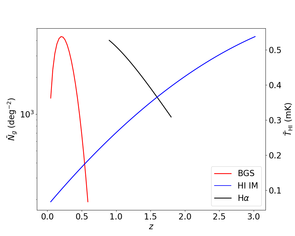
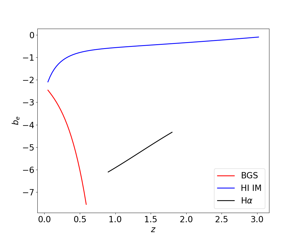
Figure 1: Top: Number density and HI temperature in mK (left), and Gaussian clustering bias (right), for the surveys. Bottom: Magnification bias (left) and evolution bias (right), for the surveys.

As described in section 2, to compute the angular power spectrum one requires astrophysical details such as number density, Gaussian clustering bias, magnification bias, evolution bias – and the noise. For Fisher forecasting of future galaxy surveys, we can use the appropriate model of the luminosity function, together with flux limits expected, to find $\bar{n}_{\rm g}$, $b_{\rm e}$ and $s$ in each redshift bin. Then fitting functions can be used to allow for different redshift binning. For IM surveys, $\bar{n}_{\rm HI}$, $b_{\rm e}$ and $s$ are survey-independent and we use a standard fitting function for the average brightness temperature $\bar{T}_{\rm HI}$ that is needed for $b_{\rm e}$. The details are given in [74]. We used the $\bar{n}_{\rm g}$ in [74] to determine fits for $\bar{N}_{\rm g}$ for the galaxy surveys. For the clustering biases, we use [63] for BGS, [77] for H$\alpha$ and [28] for HI intensity mapping. The results are shown in Figure 1 based on the following fits.

• DESI-like BGS survey:

  $$\bar{N}_{\rm g} = {z^{1.161}\exp\left[10.75-\left({}z\over 0.27\right)^{2.060}\right]}\,,$$ (3.1)

  $$b = 0.99+0.73\,z-1.29\,z^{2}+10.21\,z^{3}\,,$$ (3.2)

  $$s = 0.113+0.945\,z+0.908\,z^{2}+4.442\,z^{3}\,,$$ (3.3)

  $$b_{\rm e} = -2.25-4.02\,z+0.318\,z^{2}-14.6\,z^{3}\,.$$ (3.4)

• Euclid-like H$\alpha$ survey:

  $$\bar{N}_{\rm g} = z^{1.985}\exp\left(0.019\,z^{4}-0.052\,z^{3}+0.147\,z^{2}-3.405\,z+11.471\right)\,,$$ (3.5)

  $$b = 0.7(1+z)\,,$$ (3.6)

  $$s = 0.234+0.801\,z-0.222\,z^{2}+0.015\,z^{3}\,,$$ (3.7)

  $$b_{\rm e} = -7.29+0.470\,z+1.17\,z^{2}-0.290\,z^{3}\,.$$ (3.8)

• HI intensity mapping (any survey):

  $$\bar{T}_{\rm HI} = 0.0559+0.2324\,z-0.0241\,z^{2}~{}~{}{\rm mK}\,,$$ (3.9)

  $$b = 0.667+0.178\,z+0.050\,z^{2}\,,$$ (3.10)

  $$s = 0.4\,,$$ (3.11)

  $$b_{\rm e} = -0.32-0.11\,z+0.06\,z^{2}-\exp\left(-0.9\,z^{3}+3.12\,z^{2}-4.61\,z+0.78\right).$$ (3.12)

  Figure 1 shows that the evolution of sources in intensity mapping is less susceptible to galaxy mergers, as compared to the number counts in galaxy surveys, since intensity mapping does not resolve individual galaxies. As a result, $|b_{\rm e}^{\rm IM}|<|b_{\rm e}^{g}|$.

The intensity mapping angular power spectrum is modulated by the telescope beam, which in single-dish mode leads to a loss of small-scale transverse power:

$$C^{\rm IM\,IM}_{\ell}(z_{i},z_{j})~{}~{} \to ~{}~{}\beta_{\ell}(z_{i})\,\beta_{\ell}(z_{j})\,C^{\rm IM\,IM}_{\ell}(z_{i},z_{j})\,,$$ (3.13)

$$\beta_{\ell}(z_{i}) = \exp\left[-{\ell(\ell+1)\over 16\ln 2}\theta_{\rm b}^{2}(z_{i})\right],$$ (3.14)

where $\theta_{\rm b}=1.22\lambda_{21}(1+z)/D_{\rm d}$ is the effective field of view and $D_{\rm d}$ is the dish diameter.

Finally, we model the uncertainty due to noise, which limits how well the signal can be extracted. For galaxy surveys, the angular shot-noise power is inversely proportional to the number of galaxies observed per solid angle:

$$\mathcal{N}^{\rm g}_{\ell}(z_{i},z_{j})=\frac{1}{N_{\Omega}(z_{i})}\,\delta_{ij}~{}~{}\mbox{where}~{}~{}N_{\Omega}(z_{i})=\int{\rm d}z\,W(z,z_{i})\bar{N}_{\rm g}(z)\,.$$ (3.15)

The window function $W$ is a top-hat like window smoothed on the edges, given by [78]

$$W(z,z_{i})=\frac{1}{2\,{\tanh}({\Delta}z_{i}/2\sigma_{zi})}\left[\tanh\!\left(\!\frac{z-z_{i}+{\Delta}z_{i}/2}{\sigma_{zi}}\!\right)\!-\!\tanh\!\left(\!\frac{z-z_{i}-{\Delta}z_{i}/2}{\sigma_{zi}}\!\right)\!\right]\!,$$ (3.16)

where ${\Delta}z_{i}$ is the redshift bin size, $\sigma_{z}$ is the redshift resolution and $\sigma_{zi}=\sigma_{z}(1+z_{i})$. For HI IM experiments the main noise source is instrumental and we can neglect shot noise on the scales of interest. For single-dish surveys, the noise is [79, 80]

$$\mathcal{N_{\ell}^{\rm IM}}(z_{i},z_{j})=\frac{4\pi\,f_{\rm sky}\,T^{2}_{\rm sys}(z_{i})}{2N_{\rm d}\,t_{\rm tot}\,\Delta\nu}\,\delta_{ij}\,.$$ (3.17)

The system temperature $T_{\rm sys}$ is frequency dependent, $N_{\rm d}$ is the number of dishes, the frequency band of observation is $\Delta\nu$, the total integration time is $t_{\rm tot}$, and the sky fraction is $f_{\rm sky}=\Omega_{\rm sky}/4\pi$. We fix the scanning ratio, i.e the sky area over time. This implies that the observational time $t_{\rm tot}$, needs to be adjusted proportionally to the reduction in sky area. Further details on subtleties in the SKAO noise are given in [78].

Given the overlap between the BGS and IM2 surveys, and between the H$\alpha$ and IM1 surveys, we need to consider cross-shot noise. However, as shown in [81], the cross-shot noise is negligible and may be neglected.

The noise power spectra for the various surveys are displayed in Figure 2.

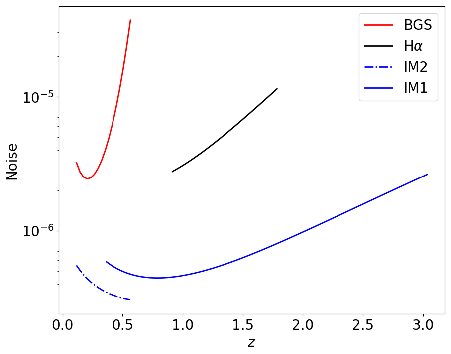
Figure 2: Shot noise for galaxy surveys and instrumental noise (normalised by $\bar{T}_{\rm HI}^{2}$) for intensity mapping surveys.

4 Primordial non-Gaussianity and relativistic effects in the multi-tracer

The scale-dependent clustering bias in Fourier space, given by (2.5), grows on large scales as ${f_{\rm NL}}H_{0}^{2}/k^{2}$, producing a power spectrum monopole $P_{\rm g}(z,k)$ that blows up on ultra-large scales. This behaviour in Fourier space is misleading, since the directly measurable signal of ${f_{\rm NL}}$ is very small. The point here is that the Fourier power spectrum is not directly observable. One has to de-project measured angular positions and redshifts into a Cartesian three-dimensional volume – which requires assuming a fiducial cosmology. The Fourier power spectrum is a derived quantity, which is also not gauge invariant. By contrast, the angular power spectrum is observable (and this is also why no Alcock-Paczynski correction is needed when analysing data via the angular power spectrum).

We illustrate this point in Figure 3, showing an example of the percentage contribution of ${f_{\rm NL}}$ to the Fourier and angular power spectra. The blow-up in the unobservable $P_{\rm g}$ is not mirrored by the behaviour of $C_{\ell}$, in which the ${f_{\rm NL}}$ contribution is only a few percent on the largest scales, where cosmic variance is typically much larger. This is why we require a multi-tracer approach to detect the signal of ${f_{\rm NL}}$.

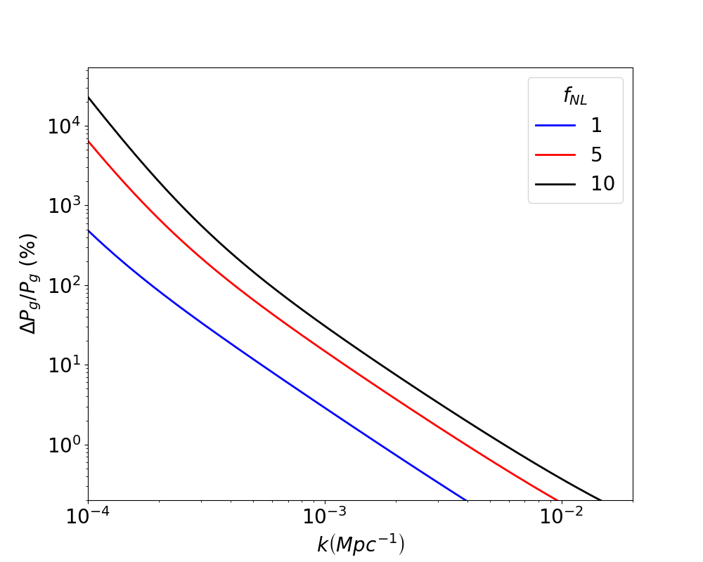
Figure 3: Percentage contribution of scale-dependent bias to the Fourier power spectrum monopole (left) and angular power spectrum (right) for an H$\alpha$ survey at $z=1.8$ with $\Delta z=0.03$.

The dominant relativistic effects are from the Doppler and lensing magnification terms. The Doppler term depends on both the magnification and evolution biases via (2.7), while the lensing term (2.12) depends only on the magnification bias. Using the fits in section 3, we show in Figure 4 the amplitude of the Doppler and lensing contributions to the observed number density and temperature contrasts.

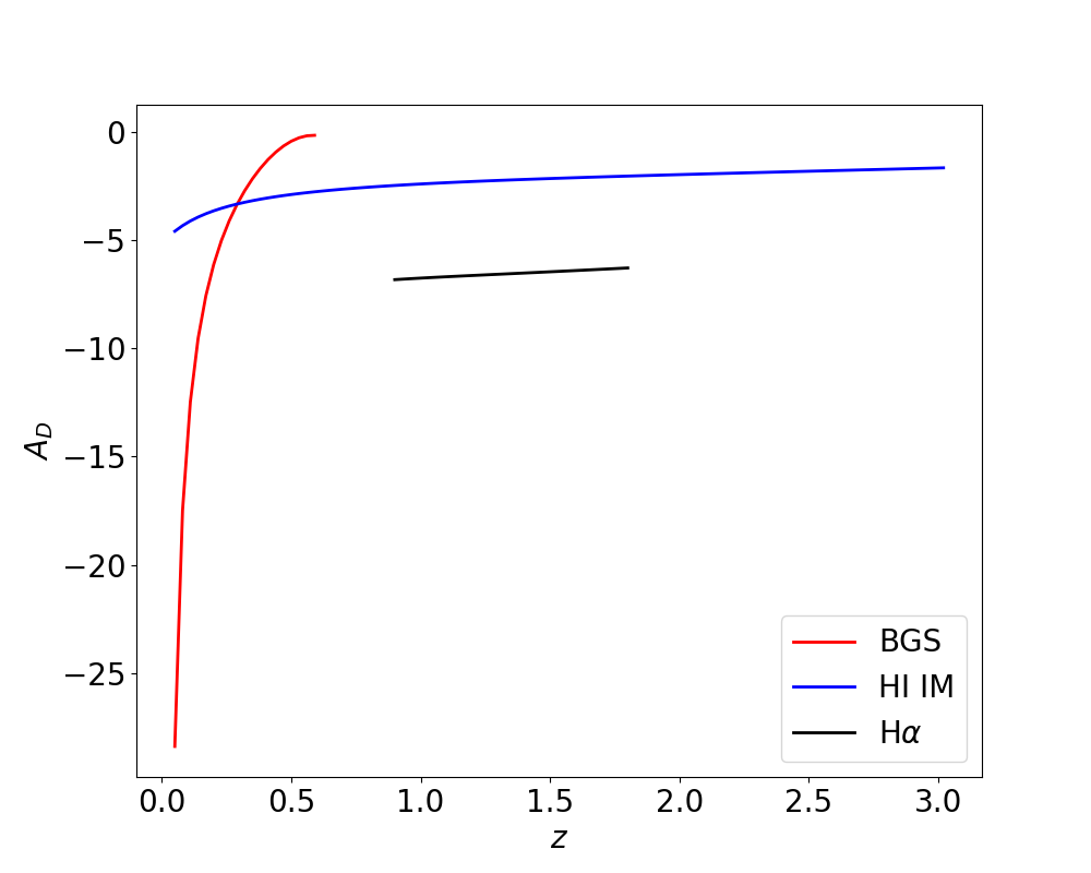
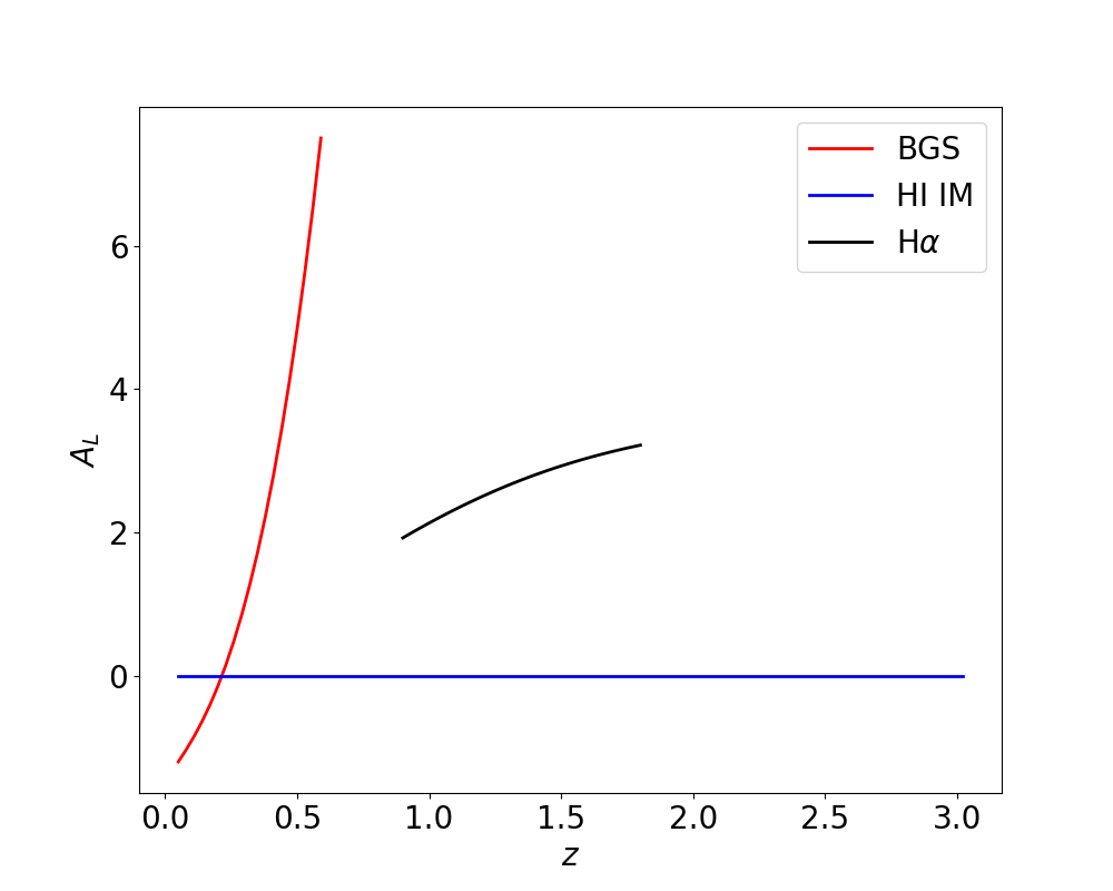
Figure 4: Coefficient of the Doppler (left) and lensing (right) contributions for the surveys.

It is apparent that the Doppler coefficient for intensity mapping is significantly smaller than for the galaxy samples. Therefore we expect HI surveys to under-perform in extracting information on the Doppler effect, compared to galaxy surveys. We also note that the Doppler amplitude is strongest at low redshift, so that the BGS survey is best placed to detect it.

The lensing coefficient vanishes for intensity mapping and is largest for the BGS survey. This does not mean that the lensing contribution for BGS is greater than for H$\alpha$, since the lensing amplitude is $|A_{\rm L}\kappa|$ and $\kappa$ will be larger at higher $z$.

For our Fisher analysis, we separate the relativistic contributions by introducing fudge factors $\varepsilon=1$ to gauge the detectability of each contribution:

$$\Delta_{A}=\delta_{A}+\Delta^{\rm RSD}+\varepsilon_{\rm D}\,\Delta^{\rm Dopp}+\varepsilon_{\rm L}\,\Delta^{\rm Lens}+\varepsilon_{\rm P}\,\Delta^{\rm Pot}\,.$$ (4.1)

In order to determine which correlations, both in single- and multi-tracer cases, add the most information, we compute the signal-to-noise of a parameter $\vartheta$, constrained by two surveys, from each correlation ${C}^{AB}_{\ell}(z^{A}_{i},z^{B}_{j})$, as

$$S^{AB}(\vartheta,z^{A}_{i},z^{B}_{j})=\left\{\sum_{\ell}\left[\frac{\partial_{\vartheta}\,{C}^{AB}_{\ell}(z^{A}_{i},z^{B}_{j})}{{\Delta C}^{AB}_{\ell}(z^{A}_{i},z^{B}_{j})}\right]^{2}\right\}^{1/2}\,,$$ (4.2)

where $A,B=1,2$ and

$${\Delta C}^{AB}_{\ell}(z^{A}_{i},z^{B}_{j})=\left\{\frac{\Gamma^{AA}_{\ell}(z^{A}_{i},z^{A}_{j})\Gamma^{BB}_{\ell}(z^{B}_{i},z^{B}_{j})+\left[\Gamma^{AB}_{\ell}(z^{A}_{i},z^{B}_{j})\right]^{2}}{(2\ell+1)f_{\rm sky}}\right\}^{1/2}\,,$$ (4.3)

with

$$\Gamma^{AB}_{\ell}=C^{AB}_{\ell}+{\mathcal{N}}^{AB}_{\ell}\,,$$ (4.4)

where the noise is given by (3.15) for galaxy surveys and (3.17) for IM.

Figure 5: Signal-to-noise $S^{AB}(\theta,z^{A}_{i},z^{B}_{j})$ for the Doppler contribution ($\theta=\varepsilon_{\rm D}$) (left) and the lensing magnification contribution ($\theta=\varepsilon_{\rm L}$) (right). Top panels: $1\otimes 2={\rm IM2}\otimes{\rm BGS}$ for $0.35<z<0.56$. Bottom panels: $1\otimes 2={\rm IM1}\otimes{\rm H}\alpha$ for $0.90<z<1.15$. Colour bar shows the signal-to-noise.

As we confirm below, the potential terms are very poorly constrained, and we set $\varepsilon_{\rm P}=0$ in this discussion. In Figure 5 we show examples of $S^{AB}$ for $\vartheta=\varepsilon_{\rm D}$ (left) and $\vartheta=\varepsilon_{\rm L}$ (right) using both low-redshift (top) and high-redshift (bottom) survey pairs. The axes indicate which $z$-bins are correlated, where $z^{1}_{i}$ is the $i$-bin of SKAO IM2 (top panels) and IM1 (bottom panels), while $z^{2}_{i}$ corresponds to BGS (top panels) and H$\alpha$ (bottom panels). For the multi-tracer combination $1\otimes 2={\rm IM2}\otimes{\rm BGS}$ (top panels) we use the redshift range $0.35<z<0.41$, and for $1\otimes 2={\rm IM1}\otimes{\rm H}\alpha$ (bottom panels), we use $0.9<z<1.12$. In both cases a bin-width $\Delta z=0.03$ is used. The colour bar shows the signal-to-noise $S^{AB}$ of the parameter for each pair $(z^{A}_{i},z^{B}_{j})$.

The plots show that the bulk of the information on $\varepsilon_{\rm D}$ comes from the cross-spectra, which contribute 3–5 times more than the individual surveys. This contribution is mainly from the cross-tracer spectra, although at low redshift it is also marginally from cross-correlations between consecutive redshift bins of the same tracer. The latter feature is the basis of the estimator constructed in [82], which is the angular power spectrum counterpart of the Doppler dipole in the 2-point correlation function [49]. Although there is some residual information in the low-redshift BGS-BGS correlations, the bulk clearly comes from the off-diagonal, i.e. the cross-tracer correlations. BGS has most information on the Doppler term, given the $1/\chi$ term in (2.7) (see Figure 4).

In the case of lensing magnification, the analysis is slightly different. Firstly, IM has no lensing magnification contribution ($A_{\rm L}=0$). However, IM can act as a lens of background galaxies in BGS and H$\alpha$. In both cases, we see that the furthest off-diagonal cross-bin correlations are the ones that provide most information on $\varepsilon_{\rm L}$. As expected this comes from the lower redshift field lensing the higher redshift field. For this reason, when the higher redshift field is traced by IM, no information is obtained – as seen in the right column of Figure 5. We also see that most information on $\varepsilon_{\rm L}$ is obtained by galaxy surveys on their own, especially at high redshift. In fact, for the H$\alpha$ survey, cross-correlations with an IM survey seem to be irrelevant for lensing. Most information lives in the furthest off-diagonal cross-bin correlations of H$\alpha$-H$\alpha$.

Having gained qualitative insights into the multi-tracer precision on ${f_{\rm NL}}$ and relativistic effects, we turn now to the quantitative estimate of constraints via Fisher forecasting. We will also include constraints on the standard cosmological parameters.

The multi-tracer Fisher matrix for angular power spectra is defined as follows [24, 25, 81]:

$$F_{{\vartheta}_{\alpha}{\vartheta}_{\beta}}=\sum_{\ell_{\rm min}}^{\ell_{\rm max}}\frac{(2\ell+1)}{2}f_{\rm sky}\,{\rm Tr}\Big{[}\big{(}\partial_{{\vartheta}_{\alpha}}\bm{C}_{\ell}\big{)}\,\bm{\Gamma}_{\ell}^{-1}\big{(}\partial_{{\vartheta}_{\beta}}\bm{C}_{\ell}\big{)}\,\bm{\Gamma}_{\ell}^{-1}\Big{]}\,,$$ (4.5)

where $\vartheta_{\alpha}$ are the parameters and

$$\bm{\Gamma}_{\ell}=\bm{C}_{\ell}+\bm{\mathcal{N}}_{\ell}\,.$$ (4.6)

For $N$ tracers:

$$\bm{C}_{\ell}=\begin{bmatrix}{C}^{11}_{\ell}(z^{1}_{i},z^{1}_{j})&~{}~{}~{}{C}^{12}_{\ell}(z^{1}_{i},z^{2}_{j})&~{}~{}~{}\cdots&~{}~{}~{}{C}^{1N}_{\ell}(z^{1}_{i},z^{N}_{j})\\ &&&\\ ~{}~{}~{}\cdots&~{}~{}~{}\cdots&~{}~{}~{}\cdots&~{}~{}~{}\cdots\\ &&&\\ {C}^{N1}_{\ell}(z^{N}_{i},z^{1}_{j})&~{}~{}~{}{C}^{N2}_{\ell}(z^{N}_{i},z^{2}_{j})&~{}~{}~{}\cdots&~{}~{}~{}{C}^{NN}_{\ell}(z^{N}_{i},z^{N}_{j})\end{bmatrix}\,,$$ (4.7)

while the noise is the diagonal matrix

$$\bm{\mathcal{N}}_{\ell}=\begin{bmatrix}{\mathcal{N}}^{11}_{\ell}(z^{1}_{i},z^{1}_{j})&~{}~{}~{}0&~{}~{}~{}\cdots&~{}~{}~{}0\\ &&&\\ ~{}~{}~{}\cdots&~{}~{}~{}\cdots&~{}~{}~{}\cdots&~{}~{}~{}\cdots\\ &&&\\ 0&~{}~{}~{}0&~{}~{}~{}\cdots&~{}~{}~{}{\mathcal{N}}^{NN}_{\ell}(z^{N}_{i},z^{N}_{j})\end{bmatrix}\,,$$ (4.8)

where we use (3.15) for galaxy surveys and (3.17) for intensity mapping. In the Fisher matrix summation we take $\ell_{\rm min}=5$, while $\ell_{\rm max}$ is redshift dependent. We follow [78] and impose

$$\ell_{\rm max}(z_{i})=\chi(z_{i})k_{\rm nl}(z_{i})\,,$$ (4.9)

where $k_{\rm nl}(z)=0.2(1+z)^{2/(2+n_{s})}~{}h\,{\rm Mpc}^{-1}$ [83], the scale marking the breakdown of a perturbative analysis of matter clustering.

In our forecasts we consider the set of parameters

$${\vartheta}_{\alpha}=\Big{\{}{f_{\rm NL}},\,\varepsilon_{\rm D},\,\varepsilon_{\rm L},\,\varepsilon_{\rm P};\,\Omega_{\rm cdm},\,\Omega_{\rm b},\,w,\,n_{s},\,H_{0},\,A_{s};\,{b_{A}(z_{i}^{A})}\Big{\}}\,.$$ (4.10)

Note that the $\varepsilon_{I}$ do not have physical meaning; instead they are used to model the detectability of the relativistic contributions. We also consider the uncertainty in the Gaussian clustering biases by marginalising over the bias in each redshift bin, $b_{A}(z_{i}^{A})$. In the single-tracer case, the forecasts are degraded by this marginalisation, but the multi-tracer analysis is only weakly affected by marginalisation over the clustering bias, consistent with [25]. We do not marginalise over the magnification and evolution biases. Instead, we consider $\varepsilon_{\rm L}$ and $\varepsilon_{\rm D}$ as rough proxies of the uncertainties in these astrophysical parameters.

5 Results

Table 2: Marginal uncertainties on ${f_{\rm NL}}$ and relativistic effects $\varepsilon_{I}$, computed by marginalising over the standard cosmological and $b_{A}(z_{i})$ only. Results are for individual surveys and their combination using the multi-tracer technique ($\otimes$). When combining low- and high-redshift information, we also consider adding their Fisher information matrices ($\oplus$). HI intensity mapping surveys are unaffected by lensing and cannot constrain $\varepsilon_{\rm L}$. (Results exclude priors.)

Redshift Survey $\sigma({f_{\rm NL}})$ $\sigma(\varepsilon_{\rm D})$ $\sigma(\varepsilon_{\rm L})$ $\sigma(\varepsilon_{\rm P})$ $0.1-0.58$ BGS 26.38 7.57 0.39 33.3 IM2 35.74 18.07 $-$ 228.3 IM2$\otimes$BGS 2.12 0.14 0.13 6.86 $0.9-1.8$ H$\alpha$ 9.34 9.08 0.04 10.0 $0.35-3.05$ IM1 4.72 6.29 $-$ 10.89 $0.60-3.05$ IM1$\otimes$H$\alpha$ 3.06 0.37 0.03 4.71 $0.1-3.05$ (IM2$\otimes$BGS)$\oplus$(IM1$\otimes$H$\alpha$) 1.70 0.13 0.03 3.79 IM2$\otimes$BGS$\otimes$IM1$\otimes$H$\alpha$ 1.55 0.13 0.02 3.47

The forecast precision on ${f_{\rm NL}}$ and relativistic effects from future surveys is computed for individual surveys, as well as for the multi-tracer case that includes all correlations between different surveys. In Table 2 we show the marginal error on ${f_{\rm NL}}$ and $\varepsilon_{I}$, marginalised over the uncertainty of the standard cosmological parameters and the biases $b_{A}(z_{i})$. This approach is in some sense closer to reality, since including the light-cone corrections in the transfer function is the correct model to use. The caveat is that this assumes the magnification and evolution biases are known. Later we will partly incorporate uncertainty in these biases by including marginalisation over the $\varepsilon_{I}$, which can be seen as a ‘marginalisation’ over the amplitude uncertainties of the relativistic terms.

The highest precision on ${f_{\rm NL}}$ from an individual survey is $\sigma({f_{\rm NL}})=4.72$ from SKAO IM1. This is not surprising since IM1 boasts the largest observed volume among the surveys. The bigger the volume, the larger the scales we observe and the more frequently we can sample correlations at scales that carry an ${f_{\rm NL}}$ signal (see Figure 3). The IM1 precision on ${f_{\rm NL}}$ can be improved by a factor of 3 by combining all low- and high-$z$ surveys (IM2$\otimes$BGS$\otimes$IM1$\otimes$H$\alpha$), resulting in $\sigma({f_{\rm NL}})=1.55$. This is significantly better than current constraints.

It is interesting to note that individually the high-$z$ surveys constrain ${f_{\rm NL}}$ remarkably better than the low-$z$, since the volumes observed are considerably larger. Individually the low-$z$ surveys cannot access as many correlations on large scales and therefore cannot constrain ${f_{\rm NL}}$ well. However, the multi-tracer eliminates cosmic variance, which enables the low-$z$ combination to access ultra-large scales and extract more ${f_{\rm NL}}$ signal. This is a clear example of how the multi-tracer works. By cancelling cosmic variance, dark matter tracer combinations in smaller overlapping volumes can perform as well as, or better than, single tracers covering large volumes. In fact the low-$z$ combination IM2$\otimes$BGS does better than its IM1$\otimes$H$\alpha$ counterpart, because of the reduced noise at lower redshift, as shown in Figure 2.

The best single-survey constraint on the Doppler contribution is again from the SKAO IM1 survey, with $\sigma(\varepsilon_{\rm D})=6.29$. This survey has the largest volume, which compensates for the small amplitude of its Doppler term (2.7). The BGS survey has the highest amplitude: its Doppler coefficient is largest (see Figure 4), and the radial peculiar velocity $\bm{n}\cdot\bm{v}$ is largest at low $z$. Nevertheless, the volume beats the amplitude for a term that has signal on ultra-large scales. As soon as we multi-trace the surveys, again we see the domination of survey volume fades away, due to cancellation of cosmic variance. Similar to ${f_{\rm NL}}$, the low-$z$ combination outperforms the high-$z$ combination by a factor of nearly 3, because of the lower noise at low $z$. This effect can also be seen in Figure 5. The full combination of four surveys offers a precision of $\sigma(\varepsilon_{\rm D})=0.13$, only slightly better than the low-$z$ combination. The multi-tracer improvement in precision over the best single tracer is a factor of nearly 50. This precision on the Doppler amplitude corresponds to a signal-to-noise of $\sim$8, sufficient for a detection of the Doppler term. It also suggests that we can make some constraint on the evolution bias, assuming that the magnification bias is constrained by the lensing term (see below).

HI intensity mapping is unaffected by lensing magnification and so cannot constrain the lensing term. The best single-survey constraint is from the high-redshift H$\alpha$ survey, as expected, delivering $\sigma(\varepsilon_{\rm L})=0.04$. This precision is about double that found in [84]. The reason is that we use many more redshift bins in our Fisher analyses than they use in their MCMC. Even though IM does not constrain lensing by itself, its correlation with a galaxy survey does improve the error – since galaxies at $z_{i}$ behind IM at $z_{j}<z_{i}$ are lensed by the IM. This is confirmed by Figure 5. As a result, IM2$\otimes$BGS improves the BGS-only lensing constraint by a factor more than 2, while IM2$\otimes$H$\alpha$ improves on H$\alpha$-only by $\sim$25%. The correlation of all four surveys improves on the H$\alpha$-only constraint by a factor of 2, with $\sigma(\varepsilon_{\rm L})=0.02$. This is a high enough precision to place reasonable constraints on the magnification bias $s$. According to [39], we need to know $s(z)$ within $5-10\%$ accuracy to avoid systematic parameter biases.

Finally, we computed the combined uncertainty $\sigma(\varepsilon_{\rm P})$ on the relativistic potential effects. Even the full multi-tracer combination is unable to achieve $\sigma(\varepsilon_{\rm P})<1$. In other words, the potential contribution to the power spectrum is not detectable (signal-to-noise $<1$).

Table 3: Fully marginal uncertainties on ${f_{\rm NL}}$ and relativistic effects $\varepsilon_{I}$. The same as Table 2, except that $\sigma({f_{\rm NL}})$ and each $\sigma(\varepsilon_{I})$ are computed by marginalising over all other parameters, not just the standard cosmological parameters.

Redshift Survey $\sigma({f_{\rm NL}})$ $\sigma(\varepsilon_{\rm D})$ $\sigma(\varepsilon_{\rm L})$ $\sigma(\varepsilon_{\rm P})$ $0.1-0.58$ BGS 45.15 8.70 0.40 60.07 IM2 44.64 26.18 $-$ 303.32 IM2$\otimes$BGS 2.71 0.14 0.13 8.87 $0.9-1.8$ H$\alpha$ 30.73 26.9 0.05 15.51 $0.35-3.05$ IM1 6.77 9.52 $-$ 21.24 $0.6-3.05$ IM1$\otimes$H$\alpha$ 4.37 0.37 0.03 6.78 $0.1-3.05$ (IM2$\otimes$BGS)$\oplus$(IM1$\otimes$H$\alpha$) 1.71 0.13 0.03 3.84 IM2$\otimes$BGS$\otimes$IM1$\otimes$H$\alpha$ 1.55 0.13 0.03 3.51

Table 3 presents a variation of Table 2 in which we include marginalisation over ${f_{\rm NL}}$ and the relativistic parameters $\varepsilon_{I}$. As mentioned earlier, this incorporates the uncertainties on the astrophysical parameters $s$ and $b_{\rm e}$, in addition to the cosmological parameters. Comparing Table 2 with Table 3, we see that for individual surveys the constraints can be substantially degraded, especially for higher redshift surveys. One exception is lensing which is only slightly affected in single tracer. When we combine all four surveys, the constraints become insensitive to the additional marginalisation.

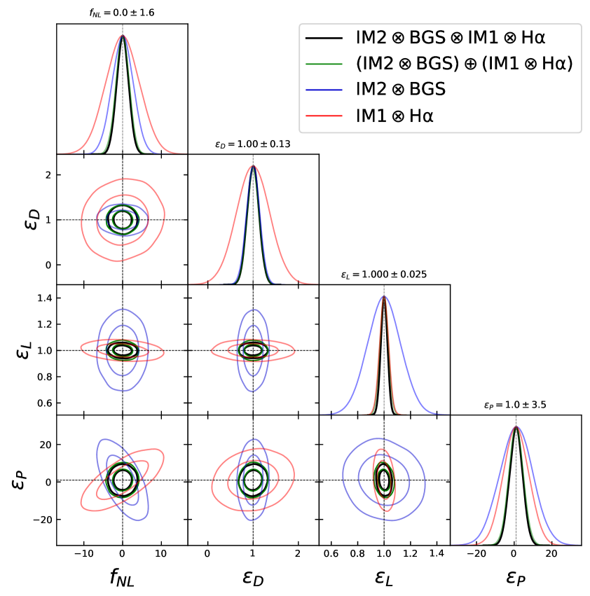
Figure 6: Contour plots of ${f_{\rm NL}}$ and relativistic parameters. The correlation of all surveys is shown in black, with dotted lines giving the fiducial values. The low-$z$ combination is shown in blue, high-$z$ in red, and the sum of their Fisher information in green. Constraints exclude priors.

Figure 6 displays the contour plots for the relativistic parameters ${f_{\rm NL}}$ and $\varepsilon_{I}$. The covariances include marginalisation over all parameters in (4.10), as in Table 3. The contours show the total correlated information (black), with its low-$z$ (blue) and high-$z$ (red) components. In green we show constraints from the simple addition of the low-$z$ and high-$z$ Fisher information. This is computationally far less expensive, although some information is lost on ${f_{\rm NL}}$ and lensing magnification. In fact, for relativistic effects, it suffices to consider cross-tracer correlations only in the overlapping footprints.

We also find that combining low-$z$ and high-$z$ samples breaks degeneracies between $\varepsilon_{\rm D}$ and $\varepsilon_{\rm L}$, and between $\varepsilon_{\rm D}$ and $\varepsilon_{\rm P}$. As an example, the degeneracy between $\varepsilon_{\rm L}$ and ${f_{\rm NL}}$ (or $\varepsilon_{\rm D}$) at low-$z$ is orthogonal to the degeneracy at high-$z$. This explains the great improvement seen in Table 3 from multi-tracer pairs at low and high redshift, to the full multi-tracer combination.

In Table 4 we give the conditional uncertainties on ${f_{\rm NL}}$ and the relativistic parameters to illustrate the robustness of the multi-tracer to uncertainty in the cosmological model. Comparing Table 3 and Table 4, it is apparent that the error for single surveys is catastrophically increased by marginalising over the cosmological model, especially at low $z$. The least affected is IM1, due to the high amount of cross-bin correlations included in the analysis. By contrast, the multi-tracer constraints are only slightly improved by not marginalising over cosmological parameters and clustering bias nuisance parameters.

Table 4: Similar to Table 2, except that we display here the conditional uncertainties on ${f_{\rm NL}}$ and relativistic effects $\varepsilon_{I}$.

Redshift Survey $\sigma({f_{\rm NL}})$ $\sigma(\varepsilon_{\rm D})$ $\sigma(\varepsilon_{\rm L})$ $\sigma(\varepsilon_{\rm P})$ $0.1-0.6$ BGS 10.56 7.41 0.39 29.79 IM2 14.17 17.17 $-$ 173.93 IM2$\otimes$BGS 2.0 0.14 0.12 6.8 $0.9-1.8$ H$\alpha$ 4.49 8.3 0.04 7.59 $0.35-3.05$ IM1 4.42 5.52 $-$ 9.25 $0.6-3.05$ IM1$\otimes$H$\alpha$ 2.72 0.37 0.03 4.43 $0.1-3.05$ (IM2$\otimes$BGS$)\oplus$(IM1$\otimes$H$\alpha$) 1.60 0.13 0.03 3.71 IM2$\otimes$BGS$\otimes$IM1$\otimes$H$\alpha$ 1.47 0.13 0.02 3.40

Systematics

In reality, we cannot perfectly extract all the observable scales from the data – there will be a loss of ultra-large-scale modes due to systematics, e.g., extinction due to Galactic dust or stellar contamination in galaxy surveys, or foreground contamination of intensity mapping. The cosmological signal from 21cm emission is several orders of magnitude lower than the galactic and extra-galactic foreground contamination. In order to extract the cosmological information, it is therefore necessary to first remove or model the systematics in galaxy and intensity mapping surveys. Recent treatments of ultra-large scale systematics are given in [85] (galaxy survey data) and [86] (21cm intensity mapping simulations). In both cases, information is lost on the largest scales, but the loss is more severe in intensity mapping.

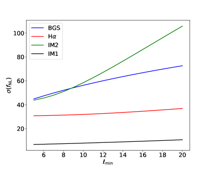
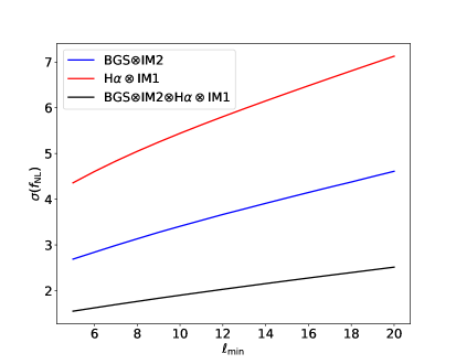
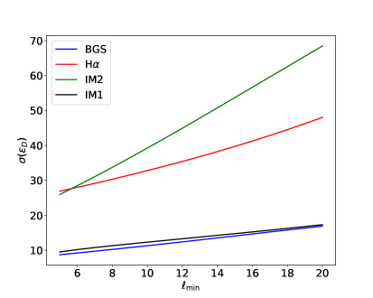
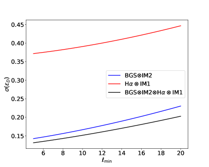
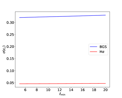
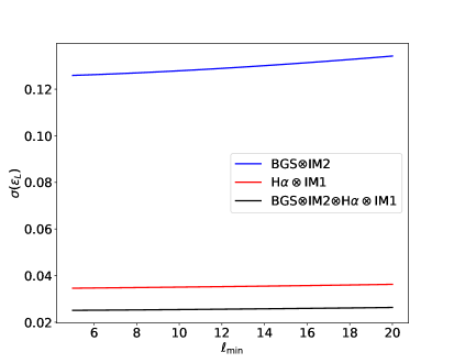
Figure 7: Uncertainty on ${f_{\rm NL}}$ (top), $\varepsilon_{\rm D}$ (middle), and $\varepsilon_{\rm L}$ (bottom) as a function of the minimum angular multipole $\ell_{\rm min}$, in the single-tracer (left panels) and multi-tracer (right panels) cases.

In order to take account of the loss of some ultra-large scale signal due to systematics, we need to impose a minimum angular multipole $\ell_{\rm min}$. For a multi-tracer analysis, the same $\ell_{\rm min}$ is used for each survey. In the case of very large sky area, $\ell_{\rm min}\sim 5$ may be feasible for intensity mapping [87], and we take this as our ‘optimistic’ minimum. Then we investigate how the constraints on ultra-large-scale parameters are affected by increasing $\ell_{\rm min}$.

The results for the non-Gaussianity and Doppler parameters are shown in Figure 7. It is clear that reducing the maximum scale (lowest $\ell$) does significantly affect the uncertainty in single surveys (left panels), for both ${f_{\rm NL}}$ (top) and $\varepsilon_{\rm D}$ (middle), as expected. By contrast, since cosmic variance is cancelled in the multi-tracer (right panels), the ultra-large scales have a smaller influence on the constraints, as previously highlighted. The constraints are much more robust to the loss of the largest scales. We conclude that our constraints should not be much affected by ultra-large scale systematics when using the multi-tracer technique.

It is worth noting that the constraints from the IM1 survey are less susceptible to increasing $\ell_{\rm min}$, because it includes extremely large-scale correlations along the line of sight, up to $(z_{i},z_{j})=(0.35,3.05)$. In addition, we find that the uncertainty on $\varepsilon_{\rm D}$ from the BGS survey closely follows IM1, because of the effect mentioned earlier: despite the reduction in observed volume at low $z$, the Doppler amplitude $A_{\rm D}$ is much bigger for BGS, and the magnitude of $\bm{n}\cdot\bm{v}$ is notably larger. The improved noise properties at low $z$ also contributes to the fact that IM2$\otimes$BGS constrains $\varepsilon_{\rm D}$ much better than IM1$\otimes$H$\alpha$.

In the case of lensing magnification, the signal does not depend significantly on ultra-large scales and we expect little effect from increasing $\ell_{\rm min}$. This expectation is confirmed by Figure 7 (bottom panels).

6 Conclusion

In this paper, we investigated how combinations of next-generation large-scale structure surveys in the optical and radio can constrain primordial non-Gaussianity and relativistic effects. Primordial non-Gaussianity is a powerful probe of the very early Universe, since its signal in the power spectrum is preserved on ultra-large scales. The relativistic effects include the contribution of lensing magnification to the number density contrast, which provides a probe of gravity and matter that is independent of the probes delivered by weak lensing shear surveys. Of the remaining relativistic effects, the Doppler effect is the most important, and provides another new probe of gravity and matter.

We reviewed the observable angular power spectra $C^{AB}_{\ell}(z^{A}_{i},z^{B}_{j})$, which naturally include all the relativistic light-cone effects, in particular the lensing magnification and Doppler effects. We chose a pair of spectroscopic surveys at low redshift and another at high redshift, which have the lowest noise in the respective parts of the electromagnetic spectrum, and which cover large areas of the sky. At low $z$ we chose a DESI-like Bright Galaxy Sample [63] in the optical and an HI intensity mapping survey with Band 2 of the SKAO MID telescope [28]. The high redshift pair is a Euclid-like H$\alpha$ spectroscopic survey [64] and HI IM with Band 1 of SKAO MID [28].

We identified which pairs of correlations are most sensitive to the lensing and Doppler effects, using a signal-to-noise estimator $S^{AB}$ in (4.2) for angular power spectra (similar to the estimator used in the 2-point correlation function by [88]). The results are summarised in Figure 5. This shows clearly that pairs $(z^{A}_{i},z^{B}_{i+1})$ are optimal for the Doppler effect and are central to the results in [49, 82]. The Doppler effect (2.7) is also more prominent at low redshifts which is broadly explained by the $1/\chi$ in its amplitude and by the growth of the radial peculiar velocity at low $z$.

On the other hand, the lensing contribution is stronger at higher redshift and is most relevant in pair correlations $(z^{A}_{1},z^{A}_{n})$, where $n$ is the total number of bins. Although this is expected, since lensing is a line-of-sight integrated effect, Figure 5 shows it in a visually intuitive manner.

Figure 5 also revealed a counter-intuitive feature – that the cross-correlation between a galaxy survey and a intensity mapping survey enhances the lensing signal, even though the intensity mapping on its own has no lensing signal. The point is that background galaxies are lensed by foreground intensity.

We then computed Fisher forecasts of the constraints on ${f_{\rm NL}}$ and the relativistic effects, for all single-tracer cases, for multi-tracer pairs at low and high $z$, and for the full multi-tracer combination of all four surveys. As expected, the full combination provides the most stringent constraints on ${f_{\rm NL}}$, improving on the state-of-the-art constraint from Planck [2] by a factor of more than 3. The lensing contribution can be detected at $\sim$2% accuracy, while the Doppler contribution can be detected with a signal-to-noise of $\sim$8.

We presented our forecasts in two scenarios. First, we assumed that the light-cone effects are perfectly modelled, i.e., the magnification and evolution biases are perfectly known. In the second case, we incorporated model uncertainties in the amplitude of the relativistic contribution to the angular power, by marginalising over these contributions. Predictably, the first scenario provides the best possible constraints. However, the second scenario constraints approach those of the first when we consider multi-tracer pairs – and even more when we combine all surveys. The multi-tracer shows one of its strengths: robustness against marginalisation.

It is notable that for the lensing contribution, most information comes from the H$\alpha$ survey alone. For the Doppler term, most of the constraints come from the low-redshift multi-tracer. For Doppler and lensing, there is sufficient sensitivity to detect their effects in the $C_{\ell}$. On the other hand, the relativistic potential terms are too small to be detected, even when combining all surveys.

In the case of ${f_{\rm NL}}$, the multi-tracer results with spectroscopic galaxy surveys delivers $\sigma({f_{\rm NL}})\sim 1.5$. This is not as good as some forecasts with photometric galaxy surveys (see e.g. [24, 28, 30]). The spectroscopic multi-tracer is not optimised for ${f_{\rm NL}}$, and this was not our focus here. On the other hand, the spectroscopic combination delivers a $\sim$10% detection of the Doppler effect, which is not possible with photometric surveys.

Finally, we stress that it is important to join the low and high redshift surveys to break degeneracies between ${f_{\rm NL}}$ and the relativistic effects, as seen in Figure 6. In addition, the multi-tracer technique provides critical robustness against the loss of information due to systematics on ultra-large scales, as shown in Figure 7.

There remains an obvious question: if we neglect the relativistic effects, what is the impact on the measured best-fit of ${f_{\rm NL}}$ and the other cosmological parameters, in single- and multi-tracer? This is tackled in a companion paper [48].

References

- [1] N. Bartolo, E. Komatsu, S. Matarrese and A. Riotto, Non-Gaussianity from inflation: Theory and observations, Phys. Rept. 402 (2004) 103 [astro-ph/0406398].
- [2] Planck collaboration, Planck 2018 results. IX. Constraints on primordial non-Gaussianity, Astron. Astrophys. 641 (2020) A9 [1905.05697].
- [3] S. Matarrese and L. Verde, The effect of primordial non-Gaussianity on halo bias, Astrophys. J. 677 (2008) L77 [0801.4826].
- [4] N. Dalal, O. Dore, D. Huterer and A. Shirokov, The imprints of primordial non-gaussianities on large-scale structure: scale dependent bias and abundance of virialized objects, Phys. Rev. D77 (2008) 123514 [0710.4560].
- [5] B. Leistedt, H. V. Peiris and N. Roth, Constraints on Primordial Non-Gaussianity from 800 000 Photometric Quasars, Phys. Rev. Lett. 113 (2014) 221301 [1405.4315].
- [6] E. Castorina et al., Redshift-weighted constraints on primordial non-Gaussianity from the clustering of the eBOSS DR14 quasars in Fourier space, JCAP 09 (2019) 010 [1904.08859].
- [7] E.-M. Mueller et al., The clustering of galaxies in the completed SDSS-IV extended Baryon Oscillation Spectroscopic Survey: Primordial non-Gaussianity in Fourier Space, 2106.13725.
- [8] T. Giannantonio, C. Porciani, J. Carron, A. Amara and A. Pillepich, Constraining primordial non-Gaussianity with future galaxy surveys, Mon. Not. Roy. Astron. Soc. 422 (2012) 2854 [1109.0958].
- [9] S. Camera, M. G. Santos, P. G. Ferreira and L. Ferramacho, Cosmology on Ultra-Large Scales with HI Intensity Mapping: Limits on Primordial non-Gaussianity, Phys. Rev. Lett. 111 (2013) 171302 [1305.6928].
- [10] A. Font-Ribera, P. McDonald, N. Mostek, B. A. Reid, H.-J. Seo and A. Slosar, DESI and other dark energy experiments in the era of neutrino mass measurements, JCAP 05 (2014) 023 [1308.4164].
- [11] S. Camera, M. G. Santos and R. Maartens, Probing primordial non-Gaussianity with SKA galaxy redshift surveys: a fully relativistic analysis, Mon. Not. Roy. Astron. Soc. 448 (2015c) 1035 [1409.8286].
- [12] D. Alonso, P. Bull, P. G. Ferreira, R. Maartens and M. Santos, Ultra large-scale cosmology in next-generation experiments with single tracers, Astrophys. J. 814 (2015) 145 [1505.07596].
- [13] A. Raccanelli, F. Montanari, D. Bertacca, O. Doré and R. Durrer, Cosmological Measurements with General Relativistic Galaxy Correlations, JCAP 1605 (2016) 009 [1505.06179].
- [14] A. Moradinezhad Dizgah, G. K. Keating and A. Fialkov, Probing Cosmic Origins with CO and [CII] Emission Lines, Astrophys. J. Lett. 870 (2019) L4 [1801.10178].
- [15] J. Fonseca and M. Liguori, Measuring ultralarge scale effects in the presence of 21 cm intensity mapping foregrounds, Mon. Not. Roy. Astron. Soc. 504 (2021) 267 [2011.11510].
- [16] R. de Putter, J. Gleyzes and O. Doré, Next non-Gaussianity frontier: What can a measurement with (fNL)1 tell us about multifield inflation?, Phys. Rev. D 95 (2017) 123507 [1612.05248].
- [17] U. Seljak, Extracting primordial non-gaussianity without cosmic variance, Phys. Rev. Lett. 102 (2009) 021302 [0807.1770].
- [18] P. McDonald and U. Seljak, How to measure redshift-space distortions without sample variance, JCAP 0910 (2009) 007 [0810.0323].
- [19] N. Hamaus, U. Seljak and V. Desjacques, Optimal Constraints on Local Primordial Non-Gaussianity from the Two-Point Statistics of Large-Scale Structure, Phys. Rev. D84 (2011) 083509 [1104.2321].
- [20] L. R. Abramo and K. E. Leonard, Why multi-tracer surveys beat cosmic variance, Mon. Not. Roy. Astron. Soc. 432 (2013) 318 [1302.5444].
- [21] L. R. Abramo, L. F. Secco and A. Loureiro, Fourier analysis of multitracer cosmological surveys, Mon. Not. Roy. Astron. Soc. 455 (2016) 3871 [1505.04106].
- [22] L. D. Ferramacho, M. G. Santos, M. J. Jarvis and S. Camera, Radio galaxy populations and the multitracer technique: pushing the limits on primordial non-Gaussianity, Mon. Not. Roy. Astron. Soc. 442 (2014) 2511 [1402.2290].
- [23] D. Yamauchi, K. Takahashi and M. Oguri, Constraining primordial non-Gaussianity via a multitracer technique with surveys by Euclid and the Square Kilometre Array, Phys. Rev. D90 (2014) 083520 [1407.5453].
- [24] D. Alonso and P. G. Ferreira, Constraining ultralarge-scale cosmology with multiple tracers in optical and radio surveys, Phys. Rev. D92 (2015) 063525 [1507.03550].
- [25] J. Fonseca, S. Camera, M. Santos and R. Maartens, Hunting down horizon-scale effects with multi-wavelength surveys, Astrophys. J. 812 (2015) L22 [1507.04605].
- [26] J. Fonseca, R. Maartens and M. G. Santos, Probing the primordial Universe with MeerKAT and DES, Mon. Not. Roy. Astron. Soc. 466 (2017) 2780 [1611.01322].
- [27] J. Fonseca, R. Maartens and M. G. Santos, Synergies between intensity maps of hydrogen lines, Mon. Not. Roy. Astron. Soc. 479 (2018) 3490 [1803.07077].
- [28] SKA collaboration, Cosmology with Phase 1 of the Square Kilometre Array: Red Book 2018: Technical specifications and performance forecasts, Publ. Astron. Soc. Austral. 37 (2020) e007 [1811.02743].
- [29] Z. Gomes, S. Camera, M. J. Jarvis, C. Hale and J. Fonseca, Non-Gaussianity constraints using future radio continuum surveys and the multitracer technique, Mon. Not. Roy. Astron. Soc. 492 (2020) 1513 [1912.08362].
- [30] M. Ballardini, W. L. Matthewson and R. Maartens, Constraining primordial non-Gaussianity using two galaxy surveys and CMB lensing, Mon. Not. Roy. Astron. Soc. 489 (2019) 1950 [1906.04730].
- [31] J. R. Bermejo-Climent, M. Ballardini, F. Finelli, D. Paoletti, R. Maartens, J. A. Rubiño Martín et al., Cosmological parameter forecasts by a joint 2D tomographic approach to CMB and galaxy clustering, Phys. Rev. D 103 (2021) 103502 [2106.05267].
- [32] J. Yoo, N. Hamaus, U. Seljak and M. Zaldarriaga, Going beyond the Kaiser redshift-space distortion formula: a full general relativistic account of the effects and their detectability in galaxy clustering, Phys. Rev. D86 (2012) 063514 [1206.5809].
- [33] A. Challinor and A. Lewis, The linear power spectrum of observed source number counts, Phys. Rev. D 84 (2011) 043516 [1105.5292].
- [34] C. Bonvin and R. Durrer, What galaxy surveys really measure, Phys. Rev. D84 (2011) 063505 [1105.5280].
- [35] M. Bruni, R. Crittenden, K. Koyama, R. Maartens, C. Pitrou and D. Wands, Disentangling non-Gaussianity, bias and GR effects in the galaxy distribution, Phys. Rev. D85 (2012) 041301 [1106.3999].
- [36] D. Jeong, F. Schmidt and C. M. Hirata, Large-scale clustering of galaxies in general relativity, Phys. Rev. D85 (2012) 023504 [1107.5427].
- [37] T. Namikawa, T. Okamura and A. Taruya, Magnification effect on the detection of primordial non-Gaussianity from photometric surveys, Phys. Rev. D83 (2011) 123514 [1103.1118].
- [38] S. Camera, R. Maartens and M. G. Santos, Einstein’s legacy in galaxy surveys, Mon. Not. Roy. Astron. Soc. 451 (2015) L80 [1412.4781].
- [39] C. S. Lorenz, D. Alonso and P. G. Ferreira, Impact of relativistic effects on cosmological parameter estimation, Phys. Rev. D 97 (2018) 023537 [1710.02477].
- [40] J. L. Bernal, N. Bellomo, A. Raccanelli and L. Verde, Beware of commonly used approximations. Part II. Estimating systematic biases in the best-fit parameters, JCAP 10 (2020) 017 [2005.09666].
- [41] A. Kehagias, A. Moradinezhad Dizgah, J. Noreña, H. Perrier and A. Riotto, A Consistency Relation for the Observed Galaxy Bispectrum and the Local non-Gaussianity from Relativistic Corrections, JCAP 08 (2015) 018 [1503.04467].
- [42] E. Di Dio, H. Perrier, R. Durrer, G. Marozzi, A. Moradinezhad Dizgah, J. Noreña et al., Non-Gaussianities due to Relativistic Corrections to the Observed Galaxy Bispectrum, JCAP 03 (2017) 006 [1611.03720].
- [43] K. Koyama, O. Umeh, R. Maartens and D. Bertacca, The observed galaxy bispectrum from single-field inflation in the squeezed limit, JCAP 07 (2018) 050 [1805.09189].
- [44] R. Maartens, S. Jolicoeur, O. Umeh, E. M. De Weerd and C. Clarkson, Local primordial non-Gaussianity in the relativistic galaxy bispectrum, JCAP 04 (2021) 013 [2011.13660].
- [45] E. Castorina and E. di Dio, The observed galaxy power spectrum in General Relativity, 2106.08857.
- [46] P. L. Taylor, K. Markovič, A. Pourtsidou and E. Huff, The RSD Sorting Hat: Unmixing Radial Scales in Projection, 2106.05293.
- [47] W. L. Matthewson and R. Durrer, Small scale effects in the observable power spectrum at large angular scales, 2107.00467.
- [48] J.-A. Viljoen, J. Fonseca and R. Maartens, Multi-wavelength spectroscopic probes: biases from neglecting light-cone effects, 2108.05746.
- [49] C. Bonvin, L. Hui and E. Gaztanaga, Asymmetric galaxy correlation functions, Phys. Rev. D89 (2014) 083535 [1309.1321].
- [50] F. Montanari and R. Durrer, Measuring the lensing potential with tomographic galaxy number counts, JCAP 10 (2015) 070 [1506.01369].
- [51] A. Hall and C. Bonvin, Measuring cosmic velocities with 21 cm intensity mapping and galaxy redshift survey cross-correlation dipoles, Phys. Rev. D 95 (2017) 043530 [1609.09252].
- [52] C. Bonvin, S. Andrianomena, D. Bacon, C. Clarkson, R. Maartens, T. Moloi et al., Dipolar modulation in the size of galaxies: The effect of Doppler magnification, Mon. Not. Roy. Astron. Soc. 472 (2017) 3936 [1610.05946].
- [53] F. Lepori, E. Di Dio, E. Villa and M. Viel, Optimal galaxy survey for detecting the dipole in the cross-correlation with 21 cm Intensity Mapping, JCAP 05 (2018) 043 [1709.03523].
- [54] S. Andrianomena, C. Bonvin, D. Bacon, P. Bull, C. Clarkson, R. Maartens et al., Testing General Relativity with the Doppler magnification effect, Mon. Not. Roy. Astron. Soc. 488 (2019) 3759 [1810.12793].
- [55] C. Bonvin and P. Fleury, Testing the equivalence principle on cosmological scales, JCAP 05 (2018) 061 [1803.02771].
- [56] C. Clarkson, E. M. de Weerd, S. Jolicoeur, R. Maartens and O. Umeh, The dipole of the galaxy bispectrum, Mon. Not. Roy. Astron. Soc. 486 (2019) L101 [1812.09512].
- [57] F. O. Franco, C. Bonvin and C. Clarkson, A null test to probe the scale-dependence of the growth of structure as a test of General Relativity, Mon. Not. Roy. Astron. Soc. 492 (2020) L34 [1906.02217].
- [58] E. M. de Weerd, C. Clarkson, S. Jolicoeur, R. Maartens and O. Umeh, Multipoles of the relativistic galaxy bispectrum, JCAP 05 (2020) 018 [1912.11016].
- [59] R. Maartens, S. Jolicoeur, O. Umeh, E. M. De Weerd, C. Clarkson and S. Camera, Detecting the relativistic galaxy bispectrum, JCAP 03 (2020) 065 [1911.02398].
- [60] F. Beutler and E. Di Dio, Modeling relativistic contributions to the halo power spectrum dipole, JCAP 07 (2020) 048 [2004.08014].
- [61] S. Jolicoeur, R. Maartens, E. M. De Weerd, O. Umeh, C. Clarkson and S. Camera, Detecting the relativistic bispectrum in 21cm intensity maps, JCAP 06 (2021) 039 [2009.06197].
- [62] O. Umeh, K. Koyama and R. Crittenden, Testing the equivalence principle on cosmological scales using the odd multipoles of galaxy cross-power spectrum and bispectrum, 2011.05876.
- [63] DESI Collaboration, A. Aghamousa, J. Aguilar, S. Ahlen, S. Alam, L. E. Allen et al., The DESI Experiment Part I: Science,Targeting, and Survey Design, arXiv e-prints (2016) [1611.00036].
- [64] Euclid collaboration, Euclid preparation: VII. Forecast validation for Euclid cosmological probes, Astron. Astrophys. 642 (2020) A191 [1910.09273].
- [65] D. Karagiannis, A. Lazanu, M. Liguori, A. Raccanelli, N. Bartolo and L. Verde, Constraining primordial non-Gaussianity with bispectrum and power spectrum from upcoming optical and radio surveys, Mon. Not. Roy. Astron. Soc. 478 (2018) 1341 [1801.09280].
- [66] D. Karagiannis, A. Slosar and M. Liguori, Forecasts on Primordial non-Gaussianity from 21 cm Intensity Mapping experiments, JCAP 11 (2020) 052 [1911.03964].
- [67] D. Karagiannis, J. Fonseca, R. Maartens and S. Camera, Probing primordial non-Gaussianity with the power spectrum and bispectrum of future 21 cm intensity maps, Phys. Dark Univ. 32 (2021) 100821 [2010.07034].
- [68] A. Barreira, Predictions for local PNG bias in the galaxy power spectrum and bispectrum and the consequences for constraints, 2107.06887.
- [69] O. Doré et al., Cosmology with the SPHEREX All-Sky Spectral Survey, 1412.4872.
- [70] M. Tellarini, A. J. Ross, G. Tasinato and D. Wands, Galaxy bispectrum, primordial non-Gaussianity and redshift space distortions, JCAP 06 (2016) 014 [1603.06814].
- [71] D. Gualdi, S. Novell, H. Gil-Marín and L. Verde, Matter trispectrum: theoretical modelling and comparison to N-body simulations, JCAP 01 (2021) 015 [2009.02290].
- [72] A. Barreira, G. Cabass, F. Schmidt, A. Pillepich and D. Nelson, Galaxy bias and primordial non-Gaussianity: insights from galaxy formation simulations with IllustrisTNG, JCAP 12 (2020) 013 [2006.09368].
- [73] A. Barreira, On the impact of galaxy bias uncertainties on primordial non-Gaussianity constraints, JCAP 12 (2020) 031 [2009.06622].
- [74] R. Maartens, J. Fonseca, S. Camera, S. Jolicoeur, J.-A. Viljoen and C. Clarkson, Magnification and evolution biases in large-scale structure surveys, 2107.13401.
- [75] A. Hall, C. Bonvin and A. Challinor, Testing General Relativity with 21-cm intensity mapping, Phys. Rev. D87 (2013) 064026 [1212.0728].
- [76] E. Di Dio, F. Montanari, J. Lesgourgues and R. Durrer, The CLASSgal code for Relativistic Cosmological Large Scale Structure, JCAP 1311 (2013) 044 [1307.1459].
- [77] A. Merson, A. Smith, A. Benson, Y. Wang and C. M. Baugh, Linear bias forecasts for emission line cosmological surveys, Mon. Not. Roy. Astron. Soc. 486 (2019) 5737 [1903.02030].
- [78] J. Fonseca, J.-A. Viljoen and R. Maartens, Constraints on the growth rate using the observed galaxy power spectrum, JCAP 1912 (2019) 028 [1907.02975].
- [79] L. Knox, Determination of inflationary observables by cosmic microwave background anisotropy experiments, Phys. Rev. D52 (1995) 4307 [astro-ph/9504054].
- [80] P. Bull, P. G. Ferreira, P. Patel and M. G. Santos, Late-time cosmology with 21cm intensity mapping experiments, Astrophys. J. 803 (2015) 21 [1405.1452].
- [81] J.-A. Viljoen, J. Fonseca and R. Maartens, Constraining the growth rate by combining multiple future surveys, JCAP 09 (2020) 054 [2007.04656].
- [82] J. Fonseca and C. Clarkson, Anti-symmetric clustering signals in the observed power spectrum, 2107.10803.
- [83] VIRGO Consortium collaboration, Stable clustering, the halo model and nonlinear cosmological power spectra, Mon. Not. Roy. Astron. Soc. 341 (2003) 1311 [astro-ph/0207664].
- [84] W. Cardona, R. Durrer, M. Kunz and F. Montanari, Lensing convergence and the neutrino mass scale in galaxy redshift surveys, Phys. Rev. D94 (2016) 043007 [1603.06481].
- [85] M. Rezaie et al., Primordial non-Gaussianity from the Completed SDSS-IV extended Baryon Oscillation Spectroscopic Survey I: Catalogue Preparation and Systematic Mitigation, 2106.13724.
- [86] M. Spinelli, I. P. Carucci, S. Cunnington, S. E. Harper, M. O. Irfan, J. Fonseca et al., SKAO HI Intensity Mapping: Blind Foreground Subtraction Challenge, 2107.10814.
- [87] A. Witzemann, D. Alonso, J. Fonseca and M. G. Santos, Simulated multitracer analyses with HI intensity mapping, Mon. Not. Roy. Astron. Soc. 485 (2019) 5519 [1808.03093].
- [88] G. Jelic-Cizmek, F. Lepori, C. Bonvin and R. Durrer, On the importance of lensing for galaxy clustering in photometric and spectroscopic surveys, JCAP 04 (2021) 055 [2004.12981].