Polynomials shrinkage estimators of a multivariate normal mean

Abstract

In this work, the estimation of the multivariate normal mean by different classes of shrinkage estimators is investigated. The risk associated with the balanced loss function is used to compare two estimators. We start by considering estimators that generalize the James-Stein estimator and show that these estimators dominate the maximum likelihood estimator (MLE), therefore are minimax, when the shrinkage function satisfies some conditions. Then, we treat estimators of polynomial form and prove the increase of the degree of the polynomial allows us to build a better estimator from the one previously constructed.

Keywords and Phrases: Balanced Loss Function, James-Stein estimator, multivariate Gaussian random variable, non-central chi-square distribution, shrinkage estimators.
AMS Subject Classification: Primary: 62C20, Secondary: 62H10, 62J07.

1 Introduction

The multivariate normal distribution has served as a central distribution in much of multivariate analysis. The statistical goal is to estimate the mean parameter which is of interest to many users in almost all fields. The performance of MLE method is not satisfactory, when the dimension of the parameter space is large. The drawbacks of using this method have been shown by Stein [14] and James and Stein [8]. Alternative techniques have been developed to improve the MLE; in this paper we focus our attention on shrinkage estimation method. This latter has become a very important technique for modelling data and provides useful techniques for combining data from various sources. Recent studies, in the context of shrinkage estimation, include Amin et al.[1], Yuzba et al. [15] and Hamdaoui et al. [6]. Benkhaled and Hamdaoui [3], have considered two forms of shrinkage estimators of the mean $\theta$ of a multivariate normal distribution $X\sim N_{p}\left(\theta,\sigma^{2}I_{p}\right)$ where $\sigma^{2}$ is unknown and estimated by the statistic $S^{2}\sim\sigma^{2}\chi_{n}^{2}$. Estimators that shrink the components of the usual estimator X to zero and estimators of Lindley-type, that shrink the components of the usual estimator to the random variable X. The aim is to ameliorate the results of minimaxity obtained in the published papers of estimators cited above. Hamdaoui et al. [5], have treated the minimaxity and limits of risks ratios of shrinkage estimators of a multivariate normal mean in the Bayesian case. The authors have considered the model $X\sim N_{p}\left(\theta,\sigma^{2}I_{p}\right)$ where $\sigma^{2}$ is unknown and have taken the prior law $\theta\sim N_{p}\left(\upsilon,\tau^{2}I_{p}\right)$. They constructed a modified Bayes estimator $\delta_{B}^{\ast}$ and an empirical modified Bayes estimator $\delta_{EB}^{\ast}$. When $n$ and $p$ are finite, they showed that the estimators $\delta_{B}^{\ast}$ and $\delta_{EB}^{\ast}$ are minimax. The authors have also interested in studying the limits of risks ratios of these estimators, to the MLE $X$, when $n$ and $p$ tend to infinity. The majority of these authors have been considered the quadratic loss function for computing the risk.
A goodness of fit criterion leads to an estimate which gives good fit and unbiased estimator, thus there is a need to provide a framework which combines the goodness of fit and precision of estimation formally. Zellner [16] suggested balanced losses that reply this problem. The reader is referred to Guikai et al. [4], Karamikabir et al. [10]. Sanjari Farsipour and Asgharzadeh [11] have considered the model: $X_{1},...,X_{n}$ to be a random sample from $N_{p}\left(\theta,\sigma^{2}\right)$ with $\sigma^{2}$ known and the aim is to estimate the parameter $\theta$. They studied the admissibility of the estimator of the form $a\overline{X}+b$ under the balanced loss function. Selahattin and Issam [12] introduced and derived the optimal extended balanced loss function (EBLF) estimators and predictors and discussed their performances.
In this work, we deal with the model $X\sim N_{p}\left(\theta,\sigma^{2}I_{p}\right)$, where the parameter $\sigma^{2}$ is known. Our aim is to estimate the unknown parameter $\theta$ by shrinkage estimators deduced from the MLE. The adopted criterion to compare two estimators is the risk associated to the balanced loss function. The paper is organized as follows. In Section 2, we recall some preliminaries that are useful for our main results. In the first part of Section 3, we establish the minimaxity of the estimators defined by $\delta_{a}^{(1)}=\left(1-a/\|X\|^{2}\right)X$, where $\|X\|=(\sum_{i=1}^{p}X_{i}{{}^{2}})^{1/2}$ is the euclidean norm of the vector $X=(X_{1},...,X_{p})$ in $\mathrm{R}^{p}$ and the real constant $a$ may depend on $p.$ In the second part of Section 3, we consider the estimators of polynomial form with the indeterminate $1/\|X\|^{2}$ and show that if we increase the degree of the polynomial we can build a better estimator from the one previously constructed. In Section 4, we conduct a simulation study that shows the performance of the considered estimators. We end the manuscript by giving an Appendix which contains the proofs of some our main results.

2 Preliminaries

In this section, we recall the following results that are useful in the proofs of our main results.
If $X$ is a multivariate Gaussian random $N_{p}\left(\theta,\sigma^{2}I_{p}\right)$ in $\mathrm{R}^{p}$, then $\frac{\|X\|^{2}}{\sigma^{2}}\sim\chi_{p}^{2}\left(\lambda\right)$ where $\chi_{p}^{2}\left(\lambda\right)$ denotes the non-central chi-square distribution with $p$ degrees of freedom and non-centrality parameter $\lambda=\frac{\left\|\theta\right\|^{2}}{2\sigma^{2}}$.
The following definition given in formula (1.2) by Arnold [2] will be used to calculate the expectation of functions of a non-central chi-square law’s variable.

Definition 2.1

Let $U\sim\chi_{p}^{2}\left(\lambda\right)$ be non-central chi-square with $p$ degrees of freedom and non-centrality parameter $\lambda$. The density function of $U$ is given by

$$f(x)=\sum_{k=0}^{+\infty}\frac{e^{-\frac{\lambda}{2}}(\frac{\lambda}{2})^{k}}{k!}\frac{x^{(p/2)+k-1}e^{-x/2}}{\Gamma(\frac{p}{2}+k)2^{(p/2)+k}},\ 0<x<+\infty.$$

The right hand side (RHS) of this equality is none other than the formula

$$\sum_{k=0}^{+\infty}\frac{e^{-\frac{\lambda}{2}}(\frac{\lambda}{2})^{k}}{k!}\chi_{p+2k}^{2},$$

where $\chi_{p+2k}^{2}$ is the density of the central $\chi^{2}$ distribution with $p+2k$ degrees of freedom.

To this definition we deduce that if $U\sim\chi_{p}^{2}\left(\lambda\right),$ then for any function $f:\mathrm{R}_{+}\longrightarrow\mathrm{R}$, $\chi_{p}^{2}\left(\lambda\right)$ integrable, we have

$$E\left[f(U)\right] = E_{\chi_{p}^{2}\left(\lambda\right)}\left[f(U)\right]$$ (1)

$$= \int_{\mathrm{R}_{+}}f(x)\chi_{p}^{2}\left(\lambda\right)dx$$

$$= \sum_{k=0}^{+\infty}\left[\int_{\mathrm{R}_{+}}f(x)\chi_{p+2k}^{2}dx\right]e^{-\frac{\lambda}{2}}\frac{\left(\frac{\lambda}{2}\right)^{k}}{k!}$$

$$= \sum_{k=0}^{+\infty}\left[\int_{\mathrm{R}_{+}}f(x)\chi_{p+2k}^{2}dx\right]P\left(\frac{\lambda}{2};dk\right),$$

where $P\left(\frac{\lambda}{2};dk\right)$ being the Poisson distribution of parameter $\frac{\lambda}{2}$ and $\chi_{p+2k}^{2}$ is the central chi-square distribution with $p+2k$ degrees of freedom.
The following Stein’s Lemma given in [13] will be often used in the next.

Lemma 2.2

Let $X$ be a $N\left(\upsilon,\sigma^{2}\right)$ real random variable and let $f:\mathrm{R}\longrightarrow\mathrm{R}$ be an indefinite integral of the Lebesgue measurable function, $f^{\prime}$ essentially the derivative of $f.$ Suppose also that $E\left(|f^{\prime}\left(X\right)\right|)<+\infty,$ then

$$E\left[\left(\frac{X-\upsilon}{\sigma}\right)f\left(X\right)\right]=E\left(f^{\prime}\left(X\right)\right).$$

3 Main results

In this section, we present the model $X\sim N_{p}\left(\theta,\sigma^{2}I_{p}\right)$ where $\sigma^{2}$ is known. Our aim is to estimate the unknown mean parameter $\theta$ by the shrinkage estimators under the balanced squared error loss function. For the sake of simplicity, we treat only the case when $\sigma^{2}=1$, as long as by a change of variable, any model of type $Y\sim N_{p}\left(\theta_{1},\sigma^{2}I_{p}\right)$ can be reduced to the model $Z\sim N_{p}\left(\theta_{2},I_{p}\right)$. Namely, we consider the model $X\sim N_{p}\left(\theta,I_{p}\right)$ and we want to estimate the unknown parameter $\theta$.

Definition 3.1

Suppose that $X$ is a random vector having a multivariate normal distribution $N_{p}\left(\theta,I_{p}\right)$ where the parameter $\theta$ is unknown. The balanced squared error loss function is defined as follows:

$$L_{\omega}(\delta,\theta)=\omega\|\delta-\delta_{0}\|^{2}+(1-\omega)\|\delta-\theta\|^{2},\ 0\leq\omega<1,$$ (2)

where $\delta_{0}$ is the target estimator of $\theta$, $\omega$ is the weight given to the proximity of $\delta$ to $\delta_{0}$, $1-\omega$ is the relative weight given to the precision of estimation portion and $\delta$ is a given estimator.

For more details about this loss see Jafari Jozani et al. [7], Zinodiny et al. [17] and Karamikabir and Afsahri [9].
We associate to this balanced squared error loss function the risk function defined by

$$R_{\omega}(\delta,\theta)=E(L_{\omega}(\delta,\theta)).$$

In this model, it is clear that the MLE is $X:=\delta_{0}$, its risk function is $(1-\omega)p$.
Indeed: we have

$$R_{\omega}(X,\theta) = \omega E(\|X-X\|^{2})+(1-\omega)E(\|X-\theta\|^{2})$$

$$= (1-\omega)E(\|X-\theta\|^{2}).$$

As $X\sim N_{p}\left(\theta,I_{p}\right)$, then $X-\theta\sim N_{p}\left(0,I_{p}\right)$, therefore $\|X-\theta\|^{2}\sim\chi^{2}_{p}$.
Hence, $E(\|X-\theta\|^{2})=E(\chi^{2}_{p})=p,$ and the desired result follows.
It is well known that $\delta_{0}$ is minimax and inadmissible for $p\geq 3$, thus any estimator dominates it is also minimax. We give the following Lemma, that will be used in our proofs and its proof is postponed to the Appendix.

Lemma 3.2

Let $U\sim\chi_{p}^{2}(\lambda)$ be non-central chi-square with $p$ degrees of freedom and non-centrality parameter $\lambda$ then,

• for any real numbers $s$ and $r$ where $-\frac{p}{2}<s\leq r<0,$ the real function

  $$H_{p,r,s}(\lambda)=\frac{E(U^{r})}{E(U^{s})}=\frac{\int_{R_{+}}x^{r}\chi_{p}^{2}(\lambda;dx)}{\int_{R_{+}}x^{s}\chi_{p}^{2}(\lambda;dx)}$$

  is nondecreasing on $\lambda.$

• Furthermore, if $X\sim N_{p}\left(\theta,I_{p}\right)$, we get

  $$\sup_{\|\theta\|}\left(\frac{E(\|X\|^{-2r+2})}{E(\|X\|^{-r})}\right)=2^{\frac{-r+2}{2}}\frac{\Gamma(\frac{p}{2}-r+1)}{\Gamma(\frac{p-r}{2})}.$$

3.1 James-Stein estimators and minimaxity

In 1956, Stein [14] proved a result that astonished many researchers and was catalyst an enormous and rich literature of substantial importance in statistical theory and practice. He showed that when estimating, under squared error loss, the unknown mean vector $\theta$ of a $p$-dimensional random vector $X$ having a normal distribution with identity covariance matrix, estimators of the form $\delta_{a,b}=\left(1-a/(b+\|X\|^{2})\right)X$ dominate the usual estimator $X$ for $a$ sufficiently small and $b$ sufficiently large when $p\geq 3$. In 1961, James and Stein [8] sharpened the result and gave an explicit class of dominating estimators, $\delta_{a}=\left(1-a/\|X\|^{2})\right)X$ for $0<a<2(p-2)$, and also showed that the choice on $a=p-2$ (the James-Stein estimator) is uniformly best. In this section we show the sufficient condition for which the estimator $\delta_{a}$ dominates the usual estimator $X$ under the balanced loss function $L_{\omega}$ defined in (2) and we determined the optimal value for $a$ (corresponding to the James-Stein estimator) that minimizes the risk function $R_{\omega}(\delta_{a},\theta)$.

Consider the estimator

$$\delta_{a}^{(1)}=\left(1-\frac{a}{\|X\|^{2}}\right)X=X-\frac{a}{\|X\|^{2}}X,$$ (3)

where the real constant $a$ may depend on $p.$

Proposition 3.3

Under the balanced loss function $L_{\omega}$, the risk function of the estimator $\delta_{a}^{(1)}$ given in (3) is

$$R_{\omega}(\delta_{a}^{(1)},\theta) = (1-\omega)\left[p-2a(p-2)E\left(\frac{1}{\|X\|^{2}}\right)\right]+a^{2}E\left(\frac{1}{\|X\|^{2}}\right).$$

Proof

Using the risk function associated to the balanced loss function $L_{\omega}$ defined in in (2) and the formula of the estimator $\delta_{a}^{(1)}$ given in (3), we obtain

$$R_{\omega}(\delta_{a}^{(1)},\theta) = \omega E\left(\left\|-\frac{a}{\|X\|^{2}}X\right\|^{2}\right)+(1-\omega)E\left(\left\|X-\theta-\frac{a}{\|X\|^{2}}X\right\|^{2}\right)$$

$$= a^{2}E\left(\frac{1}{\|X\|^{2}}\right)+(1-\omega)p-2a(1-\omega)E\left(\left\langle X-\theta,\frac{1}{\|X\|^{2}}X\right\rangle\right).$$

As,

$$E\left(\left\langle X-\theta,\frac{1}{\|X\|^{2}}X\right\rangle\right) = \sum^{p}_{i=1}E\left[(X_{i}-\theta_{i})\frac{1}{\|X\|^{2}}X_{i}\right]$$

Using Lemma 2.2, we get

$$E\left(\left\langle X-\theta,\frac{1}{\|X\|^{2}}X\right\rangle\right) = \sum^{p}_{i=1}E\left(\frac{\partial}{\partial X_{i}}\frac{1}{\|X\|^{2}}X_{i}\right)$$

$$= \sum^{p}_{i=1}E\left(\frac{1}{\|X\|^{2}}-\frac{2X_{i}^{2}}{\|X\|^{4}}\right)$$

$$= (p-2)E\left(\frac{1}{\|X\|^{2}}\right).$$

Then

$$R_{\omega}(\delta_{a}^{(1)},\theta) = a^{2}E\left(\frac{1}{\|X\|^{2}}\right)+(1-\omega)p-2a(1-\omega)E\left(\left\langle X-\theta,\frac{1}{\|X\|^{2}}X\right\rangle\right)$$

$$= a^{2}E\left(\frac{1}{\|X\|^{2}}\right)+(1-\omega)p-2a(1-\omega)(p-2)E\left(\frac{1}{\|X\|^{2}}\right)$$

$$= (1-\omega)\left[p-2a(p-2)E\left(\frac{1}{\|X\|^{2}}\right)\right]+a^{2}E\left(\frac{1}{\|X\|^{2}}\right).$$

 
Using the convexity on $a$ of the function $R_{\omega}(\delta_{a}^{(1)},\theta)$, the optimal value for $a$ that minimizes the risk function $R_{\omega}(\delta_{a}^{(1)},\theta)$, is

$$\widehat{a}=(1-\omega)(p-2).$$ (4)

For $a=\widehat{a}$, we obtain the James-Stein estimator

$$\delta_{JS}=\delta_{\widehat{a},2}=\left(1-\frac{\widehat{a}}{\|X\|^{2}}\right)X.$$ (5)

From Proposition 3.3, the risk function of $\delta_{JS}$ is

$$R_{\omega}(\delta_{JS},\theta)=(1-\omega)p-(p-2)^{2}(1-\omega)^{2}E\left(\frac{1}{p-2+2K}\right),$$ (6)

where $K\sim P\left(\frac{\|\theta\|^{2}}{2}\right)$.
From the formula (6), we note that $R_{\omega}(\delta_{JS},\theta)\leq(1-\omega)p=R_{\omega}(X,\theta),$ then $\delta_{JS}$ dominates the MLE $X,$ therefore it is also minimax.

3.2 Polynomials shrinkage estimators

Since the estimator $\delta_{a}=X-a\frac{1}{\|X\|^{2}}X$ dominates the MLE $X$ for certain values of $a$, we think to add the term $b(\frac{1}{\|X\|^{2}})^{2}X$ to the James-Stein estimator $\delta_{JS}$ to obtain an estimator that outperforms $\delta_{JS}$, then we construct the classes of shrinkage estimators which dominate the James-Stein estimator $\delta_{JS}$. Our main idea is to add each time a term of the form $\gamma(1/\|X\|^{2})^{m}X$ where $\gamma$ is a real constant may depend on $p$ and the parameter $m$ is integer, and we construct the estimators which dominate the estimators of the class defined previously. Thus in this section we deal with the shrinkage estimators of polynomial form with the indeterminate $1/\|X\|^{2}$.

Let the estimator

$$\delta_{b}^{(2)} = \delta_{JS}+b\left(\frac{1}{\|X\|^{2}}\right)^{2}X$$ (7)

$$= X-(1-\omega)(p-2)\frac{1}{\|X\|^{2}}X+b\left(\frac{1}{\|X\|^{2}}\right)^{2}X,$$

where the real constant $b$ may depend on $p.$

Proposition 3.4

Under the balanced loss function $L_{\omega}$, the risk function of the estimator $\delta_{b}^{(2)}$ given in (7) is

$$R_{\omega}(\delta_{b}^{(2)},\theta) = R_{\omega}(\delta_{JS},\theta)-4b(1-\omega)E\left(\frac{1}{\|X\|^{4}}\right)+b^{2}E\left(\frac{1}{\|X\|^{6}}\right).$$

Proof

Using the risk function associated to the balanced loss function $L_{\omega}$ defined in in (2) and the formula of the estimator $\delta_{b}^{(2)}$ given in (7), we get

$$R_{\omega}(\delta_{b}^{(2)},\theta) = \omega E\left(\left\|\delta_{JS}+b\frac{1}{\|X\|^{2}}X-X\right\|^{2}\right)+(1-\omega)E\left(\left\|\delta_{JS}+b\frac{1}{\|X\|^{2}}X-\theta\right\|^{2}\right)$$

$$= \omega E\left(\left\|\delta_{JS}-X\right\|^{2}+b^{2}\frac{1}{(\|X\|^{2})^{3}}+2\left\langle\delta_{JS}-X,b\frac{1}{(\|X\|^{2})^{2}}X\right\rangle\right)$$

$$+ (1-\omega)E\left(\left\|\delta_{JS}-\theta\right\|^{2}+b^{2}\frac{1}{(\|X\|^{2})^{3}}+2\left\langle\delta_{JS}-\theta,b\frac{1}{(\|X\|^{2})^{2}}X\right\rangle\right)$$

$$= R_{\omega}(\delta_{JS},\theta)+b^{2}E\left(\frac{1}{(\|X\|^{2})^{3}}\right)-2b\omega(1-\omega)(p-2)E\left(\frac{1}{(\|X\|^{2})^{2}}\right)$$

$$+ 2(1-\omega)E\left(\left\langle X-\theta-(1-\omega)(p-2)\frac{1}{\|X\|^{2}}X,b\frac{1}{(\|X\|^{2})^{2}}X\right\rangle\right)$$

$$= R_{\omega}(\delta_{JS},\theta)+b^{2}E\left(\frac{1}{\|X\|^{6}}\right)-2b\omega(1-\omega)(p-2)E\left(\frac{1}{\|X\|^{4}}\right)$$

$$+ 2b(1-\omega)\sum^{p}_{i=1}E\left((X_{i}-\theta_{i})\frac{X_{i}}{\|X\|^{4}}\right)-2b(1-\omega)^{2}(p-2)E\left(\frac{1}{\|X\|^{4}}\right).$$

Using Lemma 2.2, we get

$$\sum^{p}_{i=1}E\left((X_{i}-\theta_{i})\frac{X_{i}}{\|X\|^{4}}\right) = \sum^{p}_{i=1}E\left(\frac{\partial}{\partial X_{i}}\frac{X_{i}}{\|X\|^{4}}\right)$$

$$= \sum^{p}_{i=1}E\left(\frac{1}{\|X\|^{4}}-4\frac{X_{i}^{2}}{\|X\|^{6}}\right)$$

$$= (p-4)E\left(\frac{1}{\|X\|^{4}}\right).$$

Then,

$$R_{\omega}(\delta_{b}^{(2)},\theta) = R_{\omega}(\delta_{JS},\theta)+b^{2}E\left(\frac{1}{\|X\|^{6}}\right)-2b\omega(1-\omega)(p-2)E\left(\frac{1}{\|X\|^{4}}\right)$$

$$+ 2b(1-\omega)(p-4)E\left(\frac{1}{\|X\|^{4}}\right)-2b(1-\omega)^{2}(p-2)E\left(\frac{1}{\|X\|^{4}}\right)$$

$$= R_{\omega}(\delta_{JS},\theta)-4b(1-\omega)E\left(\frac{1}{\|X\|^{4}}\right)+b^{2}E\left(\frac{1}{\|X\|^{6}}\right).$$

 

Theorem 3.5

Under the balanced loss function $L_{\omega}$, the estimator $\delta_{b}^{(2)}$ with $p>6$ and

$$b=2(1-\omega)(p-6),$$

dominates the James-Stein estimator $\delta_{JS}.$

Proof

Using the Proposition 3.4, we have

$$R_{\omega}(\delta_{b}^{(2)},\theta) = R_{\omega}(\delta_{JS},\theta)-4b(1-\omega)E\left(\frac{1}{\|X\|^{4}}\right)+b^{2}\frac{E\left(\frac{1}{\|X\|^{6}}\right)}{E\left(\frac{1}{\|X\|^{4}}\right)}E\left(\frac{1}{\|X\|^{4}}\right).$$

From ii) of Lemma 3.2, we obtain

$$\frac{E\left(\frac{1}{\|X\|^{6}}\right)}{E\left(\frac{1}{\|X\|^{4}}\right)}=\frac{E\left(\|X\|^{-6}\right)}{E\left(\|X\|^{-4}\right)}\leq 2^{\frac{-4+2}{2}}\frac{\Gamma(\frac{p}{2}-4+1)}{\Gamma(\frac{p-4}{2})}=\frac{1}{p-6}.$$

Then,

$$R_{\omega}(\delta_{b}^{(2)},\theta) \leq R_{\omega}(\delta_{JS},\theta)-4b(1-\omega)E\left(\frac{1}{\|X\|^{4}}\right)+b^{2}\frac{1}{(p-6)}E\left(\frac{1}{\|X\|^{4}}\right).$$ (8)

The optimal value for $b$ that minimizes the right hand side of the last inequality, is

$$\widehat{b}=2(1-\omega)(p-6).$$ (9)

If we replace $b$ by $\widehat{b}$ in the inequality (8), we get

$$R_{\omega}(\delta_{\widehat{b}}^{(2)},\theta) \leq R_{\omega}(\delta_{JS},\theta)-4(1-\omega)^{2}(p-6)E\left(\frac{1}{\|X\|^{4}}\right)$$

$$\leq R_{\omega}(\delta_{JS},\theta).$$

 
Now, we consider the estimator

$$\delta_{c}^{(3)} = \delta_{\widehat{b}}^{(2)}+c\left(\frac{1}{\|X\|^{2}}\right)^{3}X$$ (10)

$$= X-\widehat{a}\frac{1}{\|X\|^{2}}X+\widehat{b}\left(\frac{1}{\|X\|^{2}}\right)^{2}X+c\left(\frac{1}{\|X\|^{2}}\right)^{3}X,$$

where the constants $\widehat{a}$ and $\widehat{b}$ are given respectively in (4) and (9) and the real parameter $c$ may depend on $p.$

Proposition 3.6

Under the balanced loss function $L_{\omega}$, the risk function of the estimator $\delta_{c}^{(3)}$ given in (10) is

$$R_{\omega}(\delta_{c}^{(3)},\theta) = R_{\omega}(\delta_{\widehat{b}}^{(2)},\theta)+c^{2}E\left(\frac{1}{\|X\|^{10}}\right)+4c(1-\omega)(p-6)E\left(\frac{1}{\|X\|^{8}}\right)$$

$$- 8c(1-\omega)E\left(\frac{1}{\|X\|^{6}}\right).$$

Proof

Using the risk function associated to the balanced loss function $L_{\omega}$ defined in in (2) and the formula of the estimator $\delta_{c}^{(3)}$ given in (10), we obtain

$$R_{\omega}(\delta_{c}^{(3)},\theta) = \omega E\left(\left\|\delta_{\widehat{b}}^{(2)}+c\left(\frac{1}{\|X\|^{2}}\right)^{3}X-X\right\|^{2}\right)$$

$$+ (1-\omega)E\left(\left\|\delta_{\widehat{b}}^{(2)}+c\left(\frac{1}{\|X\|^{2}}\right)^{3}X-\theta\right\|^{2}\right)$$

$$= \omega E\left(\left\|\delta_{\widehat{b}}^{(2)}-X\right\|^{2}+c^{2}\frac{1}{(\|X\|^{2})^{5}}+2\left\langle\delta_{\widehat{b}}^{(2)}-X,c\frac{1}{(\|X\|^{2})^{3}}X\right\rangle\right)$$

$$+ (1-\omega)E\left(\left\|\delta_{\widehat{b}}^{(2)}-\theta\right\|^{2}+c^{2}\frac{1}{(\|X\|^{2})^{5}}+2\left\langle\delta_{\widehat{b}}^{(2)}-\theta,c\frac{1}{(\|X\|^{2})^{3}}X\right\rangle\right)$$

$$= R_{\omega}(\delta_{\widehat{b}}^{(2)},\theta)+c^{2}E\left(\frac{1}{(\|X\|^{2})^{5}}\right)$$

$$+ 2\omega E\left\langle-\widehat{a}\frac{1}{\|X\|^{2}}X+\widehat{b}\left(\frac{1}{\|X\|^{2}}\right)^{2}X,c\left(\frac{1}{\|X\|^{2}}\right)^{3}X\right\rangle$$

$$+ 2(1-\omega)E\left\langle X-\theta-\widehat{a}\frac{1}{\|X\|^{2}}X+\widehat{b}\left(\frac{1}{\|X\|^{2}}\right)^{2}X,c\left(\frac{1}{\|X\|^{2}}\right)^{3}X\right\rangle$$

$$= R_{\omega}(\delta_{\widehat{b}}^{(2)},\theta)+c^{2}E\left(\frac{1}{\|X\|^{10}}\right)-2c\widehat{a}E\left(\frac{1}{\|X\|^{6}}\right)$$

$$+ 2c\widehat{b}E\left(\frac{1}{\|X\|^{8}}\right)+2c(1-\omega)\sum^{p}_{i=1}E\left((X_{i}-\theta_{i})\frac{X_{i}}{\|X\|^{6}}\right).$$

Using Lemma 2.2, we get

$$\sum^{p}_{i=1}E\left((X_{i}-\theta_{i})\frac{X_{i}}{\|X\|^{6}}\right) = \sum^{p}_{i=1}E\left(\frac{\partial}{\partial X_{i}}\frac{X_{i}}{\|X\|^{6}}\right)$$

$$= (p-6)E\left(\frac{1}{\|X\|^{6}}\right).$$

Then

$$R_{\omega}(\delta_{c}^{(3)},\theta) = R_{\omega}(\delta_{\widehat{b}}^{(2)},\theta)+c^{2}E\left(\frac{1}{\|X\|^{10}}\right)-2c(1-\omega)(p-2)E\left(\frac{1}{\|X\|^{6}}\right)$$

$$+ 4c(1-\omega)(p-6)E\left(\frac{1}{\|X\|^{8}}\right)+2c(1-\omega)(p-6)E\left(\frac{1}{\|X\|^{6}}\right)$$

$$= R_{\omega}(\delta_{\widehat{b}}^{(2)},\theta)+c^{2}E\left(\frac{1}{\|X\|^{10}}\right)+4c(1-\omega)(p-6)E\left(\frac{1}{\|X\|^{8}}\right)$$

$$- 8c(1-\omega)E\left(\frac{1}{\|X\|^{6}}\right).$$

 

Theorem 3.7

Under the balanced loss function $L_{\omega}$, the estimator $\delta_{c}^{(3)}$ with $p>10$ and

$$c=2(1-\omega)(p-10)^{2},$$

dominates the estimator $\delta_{\widehat{b}}^{(2)}.$

Proof

Using the last Proposition, we have

$$R_{\omega}(\delta_{c}^{(3)},\theta) = R_{\omega}(\delta_{\widehat{b}}^{(2)},\theta)+c^{2}\frac{E\left(\frac{1}{\|X\|^{10}}\right)}{E\left(\frac{1}{\|X\|^{6}}\right)}E\left(\frac{1}{\|X\|^{6}}\right)$$

$$+ 4c(1-\omega)(p-6)\frac{E\left(\frac{1}{\|X\|^{8}}\right)}{E\left(\frac{1}{\|X\|^{6}}\right)}E\left(\frac{1}{\|X\|^{6}}\right)$$

$$- 8c(1-\omega)E\left(\frac{1}{\|X\|^{6}}\right).$$

From ii) of Lemma 3.2, we obtain

$$\frac{E\left(\frac{1}{\|X\|^{10}}\right)}{E\left(\frac{1}{\|X\|^{6}}\right)}=\frac{E\left(\|X\|^{-10}\right)}{E\left(\|X\|^{-6}\right)}\leq 2^{\frac{-6+2}{2}}\frac{\Gamma(\frac{p}{2}-6+1)}{\Gamma(\frac{p-6}{2})}=\frac{1}{(p-8)(p-10)},$$

and from i) of Lemma 3.2, we get

$$\frac{E\left(\frac{1}{\|X\|^{8}}\right)}{E\left(\frac{1}{\|X\|^{6}}\right)} = \frac{E\left((\chi_{p}^{2}(\lambda))^{-4}\right)}{E\left((\chi_{p}^{2}(\lambda))^{-3}\right)}$$

$$\leq \frac{E\left((\chi_{p}^{2})^{-4}\right)}{E\left((\chi_{p}^{2})^{-3}\right)}=\frac{2^{-4}\frac{\Gamma(\frac{p}{2}-4)}{\Gamma(\frac{p}{2})}}{2^{-3}\frac{\Gamma(\frac{p}{2}-3)}{\Gamma(\frac{p}{2})}}=\frac{1}{p-8}.$$

where $\lambda=\frac{\|\theta\|^{2}}{2}$ and $\chi_{p}^{2}$ is the central chi-square distribution with $p$ degrees of freedom. Then,

$$R_{\omega}(\delta_{c}^{(3)},\theta) \leq R_{\omega}(\delta_{\widehat{b}}^{(2)},\theta)+c^{2}\frac{1}{(p-8)(p-10)}E\left(\frac{1}{\|X\|^{6}}\right)$$ (11)

$$+ 4c(1-\omega)(p-6)\frac{1}{p-8}E\left(\frac{1}{\|X\|^{6}}\right)-8c(1-\omega)E\left(\frac{1}{\|X\|^{6}}\right)$$

$$= R_{\omega}(\delta_{\widehat{b}}^{(2)},\theta)+c^{2}\frac{1}{(p-8)(p-10)}E\left(\frac{1}{\|X\|^{6}}\right)$$

$$- 4c(1-\omega)\frac{p-10}{p-8}E\left(\frac{1}{\|X\|^{6}}\right).$$

The optimal value for $c$ that minimizes the right hand side of the inequality (11), is

$$\widehat{c}=2(1-\omega)(p-10)^{2}.$$ (12)

If we replace $c$ by $\widehat{c}$ in the inequality (11), we get

$$R_{\omega}(\delta_{c}^{(3)},\theta) \leq R_{\omega}(\delta_{\widehat{b}}^{(2)},\theta)-4\frac{(1-\omega)^{2}(p-10)^{3}}{p-8}E\left(\frac{1}{\|X\|^{6}}\right)$$

$$\leq R_{\omega}(\delta_{\widehat{b}}^{(2)},\theta).$$

 
Now, we consider the estimator

$$\delta_{d}^{(4)} = \delta_{\widehat{c}}^{(2)}+d\left(\frac{1}{\|X\|^{2}}\right)^{4}X$$ (13)

$$= X-\widehat{a}\frac{1}{\|X\|^{2}}X+\widehat{b}\left(\frac{1}{\|X\|^{2}}\right)^{2}X+\widehat{c}\left(\frac{1}{\|X\|^{2}}\right)^{3}X+d\left(\frac{1}{\|X\|^{2}}\right)^{4}X,$$

where the constants $\widehat{a}$ and $\widehat{b}$ and $\widehat{c}$ are given respectively in (4), (9) and (12) and the real parameter $d$ may depend on $p$. Using the same technique used in the proofs of Proposition (3.6) and theorem (3.7), we obtain the following results.

Proposition 3.8

Under the balanced loss function $L_{\omega}$, the risk function of the estimator $\delta_{d}^{(4)}$ given in (13) is

$$R_{\omega}(\delta_{d}^{(4)},\theta) = R_{\omega}(\delta_{\widehat{c}}^{(3)},\theta)+d^{2}E\left(\frac{1}{\|X\|^{14}}\right)+4d(1-\omega)(p-10)^{2}E\left(\frac{1}{\|X\|^{12}}\right)$$

$$+ 4d(1-\omega)(p-6)E\left(\frac{1}{\|X\|^{10}}\right)-12d(1-\omega)E\left(\frac{1}{\|X\|^{8}}\right),$$

Theorem 3.9

Under the balanced loss function $L_{\omega}$, the estimator $\delta_{d}^{(4)}$ with $p>14$ and

$$d=2(1-\omega)(p^{2}-28p+188)(p-14)$$

dominates the estimator $\delta_{\widehat{c}}^{(3)}$.

4 Simulation results

We recall the form of the James-Stein estimator $\delta_{JS}$ given in (5). Its risk function associated to the balanced squared error loss function $L_{\omega}$ is given by the formula (6).
We also recall the estimators $\delta_{b}^{(2)},$ $\delta_{c}^{(3)},$ and $\delta_{d}^{(4)},$ given respectively in (7), (10) and (13) with $b=(1-\omega)(p-6),$ $c=(1-\omega)(p-10)^{2}$ and $d=2(1-\omega)(p^{2}-28p+188)(p-14)$. Their risk functions associated to the balanced squared error loss function $L_{\omega}$ are obtained by replacing the constants $b,c$ and $d$ in the Propositions (3.4), (3.6) and (3.8) respectively.

In this section, taking the values of the constants $b,$ $c$ and $d$ given above. In the first part of this section, we present the graphs of the risks ratios of the estimators $\delta_{JS},$ $\delta_{b}^{(2)}$ and $\delta_{c}^{(3)}$, to the MLE $X$ denoted respectively: $\frac{R_{\omega}(\delta_{JS},\theta)}{R_{\omega}(X,\theta)},$ $\frac{R_{\omega}(\delta_{b}^{(2)},\theta)}{R_{\omega}(X,\theta)}$ and $\frac{R_{\omega}(\delta_{c}^{(3)},\theta)}{R_{\omega}(X,\theta)}$ as function of $\lambda=\left\|\theta\right\|^{2},$ for various values of $p$ and $\omega.$ In the second part of this section, we present two groups of tables. The first group containing the values of risks ratios $\frac{R_{\omega}(\delta_{JS},\theta)}{R_{\omega}(X,\theta)},$ $\frac{R_{\omega}(\delta_{b}^{(2)},\theta)}{R_{\omega}(X,\theta)}$ and $\frac{R_{\omega}(\delta_{c}^{(3)},\theta)}{R_{\omega}(X,\theta)}$ as a function of variable $\lambda=\left\|\theta\right\|^{2},$ for various values of $p$ and $\omega.$ In the second group we give the values of risks ratios $\frac{R_{\omega}(\delta_{c}^{(3)},\theta)}{R_{\omega}(X,\theta)}$ and $\frac{R_{\omega}(\delta_{d}^{(4)},\theta)}{R_{\omega}(X,\theta)}$ as a function of variable $\lambda=\left\|\theta\right\|^{2},$ for various values of $p$ and $\omega.$

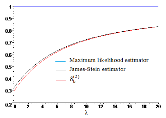
Figure 1: Graph of risks ratios $\frac{R_{\omega}(\delta_{JS},\theta)}{R_{\omega}(X,\theta)}$ and $\frac{R_{\omega}(\delta_{b}^{(2)},\theta)}{R_{\omega}(X,\theta)}$ as function of $\lambda$ for $p=8$ and $\omega=0.1$

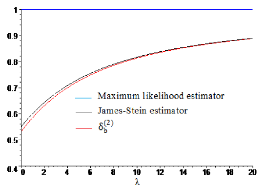
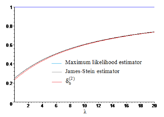
Figure 2: Graph of risks ratios $\frac{R_{\omega}(\delta_{JS},\theta)}{R_{\omega}(X,\theta)}$ and $\frac{R_{\omega}(\delta_{b}^{(2)},\theta)}{R_{\omega}(X,\theta)}$ as function of $\lambda$ for $p=8$ and $\omega=0.4$

Figure 3: Graph of risks ratios $\frac{R_{\omega}(\delta_{JS},\theta)}{R_{\omega}(X,\theta)}$ and $\frac{R_{\omega}(\delta_{b}^{(2)},\theta)}{R_{\omega}(X,\theta)}$ as function of $\lambda$ for $p=12$ and $\omega=0.1$

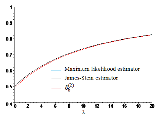
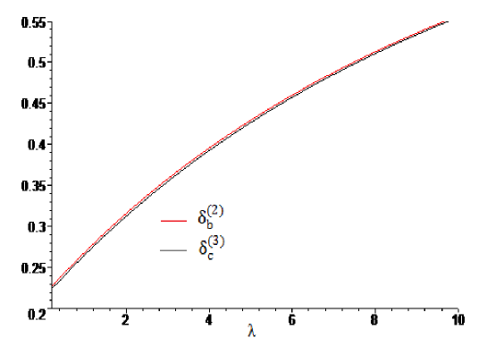
Figure 4: Graph of risks ratios $\frac{R_{\omega}(\delta_{JS},\theta)}{R_{\omega}(X,\theta)}$ and $\frac{R_{\omega}(\delta_{b}^{(2)},\theta)}{R_{\omega}(X,\theta)}$ as function of $\lambda$ for $p=12$ and $\omega=0.4$

Figure 5: Graph of risks ratios $\frac{R_{\omega}(\delta_{b}^{(2)},\theta)}{R_{\omega}(X,\theta)}$ and $\frac{R_{\omega}(\delta_{c}^{(3)},\theta)}{R_{\omega}(X,\theta)}$ as function of $\lambda$ for $p=14$ and $\omega=0.1$

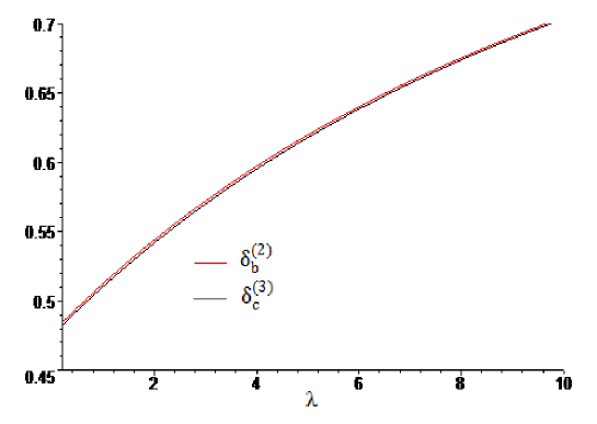
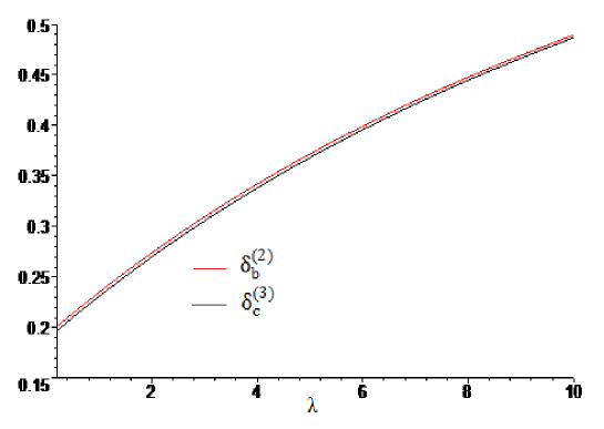
Figure 6: Graph of risks ratios $\frac{R_{\omega}(\delta_{b}^{(2)},\theta)}{R_{\omega}(X,\theta)}$ and $\frac{R_{\omega}(\delta_{c}^{(3)},\theta)}{R_{\omega}(X,\theta)}$ as function of $\lambda$ for $p=14$ and $\omega=0.4$

Figure 7: Graph of risks ratios $\frac{R_{\omega}(\delta_{b}^{(2)},\theta)}{R_{\omega}(X,\theta)}$ and $\frac{R_{\omega}(\delta_{c}^{(3)},\theta)}{R_{\omega}(X,\theta)}$ as function of $\lambda$ for $p=18$ and $\omega=0.1$

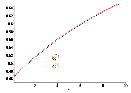
Figure 8: Graph of risks ratios $\frac{R_{\omega}(\delta_{b}^{(2)},\theta)}{R_{\omega}(X,\theta)}$ and $\frac{R_{\omega}(\delta_{c}^{(3)},\theta)}{R_{\omega}(X,\theta)}$ as function of $\lambda$ for $p=18$ and $\omega=0.4$

The previous figures show that the risks ratios $\frac{R_{\omega}(\delta_{JS},\theta)}{R_{\omega}(X,\theta)},$ $\frac{R_{\omega}(\delta_{b}^{(2)},\theta)}{R_{\omega}(X,\theta)}$ and $\frac{R_{\omega}(\delta_{c}^{(3)},\theta)}{R_{\omega}(X,\theta)}$ are less than 1, then the estimators $\delta_{JS},\delta_{b}^{(2)},$ and $\delta_{c}^{(3)}$ dominate the MLE $X$ for divers values of $p$ and $\omega,$ therefore are minimax. We note that the estimator $\delta_{b}^{(2)}$ dominates the James-Stein estimator $\delta_{JS}$ and $\delta_{c}^{(3)}$ dominates $\delta_{b}^{(2)}$ for the selected value of $p$ and $\omega$. We also observe that the gain increases if $\omega$ is near to 0 and decreases if $\omega$ is near to $1.$ The following tables illustrate this note. In these tables, first we give the values of the risks ratios $\frac{R_{\omega}(\delta_{JS},\theta)}{R_{\omega}(X,\theta)},$ $\frac{R_{\omega}(\delta_{b}^{(2)},\theta)}{R_{\omega}(X,\theta)}$ and $\frac{R_{\omega}(\delta_{c}^{(3)},\theta)}{R_{\omega}(X,\theta)}$ for the different values of $\lambda$, $p$ and $\omega$. The first entry is $\frac{R_{\omega}(\delta_{JS},\theta)}{R_{\omega}(X,\theta)},$ the middle entry is $\frac{R_{\omega}(\delta_{b}^{(2)},\theta)}{R_{\omega}(X,\theta)},$ and the third entry is $\frac{R_{\omega}(\delta_{c}^{(3)},\theta)}{R_{\omega}(X,\theta)}$.

Table 1: $p=14$

$\lambda$	$\omega=0.0$	$\omega=0.1$	$\omega=0.2$	$\omega=0.5$	$\omega=0.7$	$\omega=0.9$
1.2418	0.2134 0.2010 0.1973	0.2920 0.2809 0.2776	0.3707 0.3608 0.3579	0.6067 0.6005 0.5987	0.7640 0.7603 0.7592	0.9213 0.9201 0.9197
5.0019	0.3745 0.3663 0.36309	0.4371 0.4297 0.4268	0.4996 0.4930 0.4905	0.6873 0.6831 0.6815	0.8124 0.8099 0.8089	0.9374 0.9366 0.9363
10.4311	0.5218 0.5168 0.5150	0.5697 0.5652 0.5635	0.6175 0.6135 0.6120	0.7609 0.7584 0.7575	0.8565 0.8550 0.8545	0.9522 0.9517 0.9515
15.4110	0.6086 0.6052 0.6041	0.6477 0.6447 0.6437	0.6869 0.6842 0.6833	0.8043 0.8026 0.8020	0.8826 0.8816 0.8812	0.9608 0.9605 0.9604
20.0000	0.6653 0.6628 0.6621	0.6988 0.6965 0.6959	0.7322 0.7302 0.7297	0.8326 0.8314 0.8310	0.8996 0.8988 0.8986	0.9665 0.9663 0.9662

Table 2: $p=18$

$\lambda$	$\omega=0.0$	$\omega=0.1$	$\omega=0.2$	$\omega=0.5$	$\omega=0.7$	$\omega=0.9$
1.2418	0.1688 0.1608 0.1563	0.2519 0.2448 0.2406	0.3351 0.3287 0.3250	0.5844 0.5804 0.5781	0.7506 0.7482 0.7469	0.9169 0.9161 0.9156
5.0019	0.3079 0.3021 0.2980	0.3771 0.3719 0.3682	0.4463 0.4417 0.4384	0.6540 0.6511 0.6490	0.7924 0.7906 0.7894	0.9308 0.9302 0.9298
10.4311	0.4535 0.4418 0.4390	0.5011 0.4976 0.4951	0.5565 0.5534 0.5512	0.7228 0.7209 0.7195	0.8337 0.8325 0.8317	0.9446 0.9442 0.9439
15.4110	0.5327 0.5299 0.5280	0.5794 0.5769 0.5752	0.6261 0.6239 0.6224	0.7663 0.7649 0.7640	0.8598 0.8590 0.8584	0.9533 0.9530 0.9528
20.0000	0.5923 0.5901 0.5888	0.6331 0.6311 0.6299	0.6738 0.6721 0.6710	0.7961 0.7951 0.7944	0.8777 0.8770 0.8766	0.9592 0.9590 0.9589

In tables 1 and 2, we note that: if $\omega$ and $\lambda=\|\theta\|^{2}$ are small, the gain of the risks ratios $\frac{R_{\omega}(\delta_{JS},\theta)}{R_{\omega}(X,\theta)},$ $\frac{R_{\omega}(\delta_{b}^{(2)},\theta)}{R_{\omega}(X,\theta)}$ and $\frac{R_{\omega}(\delta_{c}^{(3)},\theta)}{R_{\omega}(X,\theta)}$ is very important. Also, if the values of $\omega$ and $\lambda$ increase, the gain decreases and approaches to zero, a little improvement is then obtained. We also observe that, if the values of $p$ increase, the gain increases and this for each fixed value of $\omega$. We also see that, if the values of $p$ are large, the gain is large and consequently we obtain more improvement. We conclude that, the gain is important when the parameters $p$ and $\lambda$ are large and $\omega$ is near to $0$. As seen above, the gain of the risks ratios is influenced by various values of $p$, $\omega$ and $\lambda$.

Now, we give the tables that present the values of risks ratios $\frac{R_{\omega}\left(\delta_{c}^{(3)},\theta\right)}{R_{\omega}(X,\theta)}$ and $\frac{R_{\omega}\left(\delta_{d}^{(4)},\theta\right)}{R_{\omega}(X,\theta)}$ for various values of $\lambda$, $p$ and $\omega.$ The first entry is $\frac{R_{\omega}(\delta_{c}^{(3)},\theta)}{R_{\omega}(X,\theta)},$ and the second entry is $\frac{R_{\omega}(\delta_{d}^{(4)},\theta)}{R_{\omega}(X,\theta)}$.

Table 3: $p=20$

$\lambda$	$\omega=0.0$	$\omega=0.1$	$\omega=0.2$	$\omega=0.5$	$\omega=0.7$	$\omega=0.9$
1.2418	0.1419 0.1414	0.2277 0.2274	0.3135 0.3134	0.5709 0.5713	0.7426 0.7432	0.9142 0.9152
5.0019	0.2738 0.2732	0.3464 0.3459	0.4190 0.4187	0.6369 0.6368	0.7821 0.7822	0.9274 0.9277
10.4311	0.4091 0.4087	0.4682 0.4679	0.5273 0.5270	0.7045 0.7044	0.8227 0.8227	0.9409 0.9410
15.4110	0.4969 0.4967	0.5472 0.5470	0.5975 0.5973	0.7484 0.7483	0.8491 0.8490	0.9497 0.9497
20.0000	0.5581 0.5579	0.6022 0.6021	0.6464 0.6463	0.7790 0.7790	0.8674 0.8674	0.9558 0.9558

Table 4: $p=24$

$\lambda$	$\omega=0.0$	$\omega=0.1$	$\omega=0.2$	$\omega=0.5$	$\omega=0.7$	$\omega=0.9$
1.2418	0.1201 0.1191	0.2081 0.2074	0.2961 0.2957	0.5600 0.5606	0.7360 0.7372	0.9120 0.9138
5.0019	0.2359 0.2348	0.3123 0.3114	0.3887 0.3880	0.6180 0.6178	0.7708 0.7710	0.9236 0.9242
10.4311	0.3604 0.3596	0.4244 0.4237	0.4883 0.4877	0.6802 0.6799	0.8081 0.8081	0.9360 0.9362
15.4110	0.4448 0.4442	0.5003 0.4998	0.5558 0.5554	0.7224 0.7222	0.8334 0.8333	0.9445 0.9445
20.0000	0.5055 0.5051	0.5549 0.5546	0.6044 0.6041	0.7527 0.7526	0.8516 0.8516	0.9505 0.9505

In tables 3 and 4, we note that: the gain are less than the gain in the tables 1 and 2, namely there is a little improvement in the domination of the estimator $\delta_{d}^{(4)}$ to the estimator $\delta_{c}^{(3)}$ if comparing with the improvement of the estimator $\delta_{b}^{(2)}$ to the James-Stein estimator or the improvement of the estimator $\delta_{c}^{(3)}$ to the estimator $\delta_{b}^{(2)}$. We can also remark that the parameters $p$, $\omega$ and $\lambda$ have the same influence to the risks ratios, as in the tables 1 and 2.

5 Appendix

Proof

(Proof of Lemma 3.2) First, we show that, for any real $\upsilon$

$$\frac{\partial}{\partial\lambda}E(U^{\upsilon})=\frac{\partial}{\partial\lambda}\int_{R_{+}}x^{\upsilon}\chi_{p}^{2}(\lambda;dx)=\upsilon 2^{\upsilon-1}\sum^{+\infty}_{k=0}\frac{\Gamma(\frac{p}{2}+\upsilon+k)}{\Gamma(\frac{p}{2}+1+k)}P\left(\frac{\lambda}{2};dk\right),$$

where $P(\frac{\lambda}{2})$ being the Poisson distribution of parameter $\frac{\lambda}{2}$.
Using the formula (1) we have, for any real $\upsilon$

$$E(U^{\upsilon})=E[(\chi_{p}^{2}(\lambda))^{\upsilon}]=E[(\chi_{p+2K}^{2})^{\upsilon}]=2^{\upsilon}E\left[\frac{\Gamma(\frac{p}{2}+K+\upsilon)}{\Gamma(\frac{p}{2}+K)}\right],$$ (14)

where $K\sim P(\frac{\lambda}{2})$. Then

$$\frac{\partial}{\partial\lambda}E(U^{\upsilon}) = \frac{\partial}{\partial\lambda}\int_{R_{+}}x^{\upsilon}\chi_{p}^{2}(\lambda;dx)$$

$$= 2^{\upsilon}\sum^{+\infty}_{k=0}\left[\frac{\Gamma(\frac{p}{2}+k+\upsilon)}{\Gamma(\frac{p}{2}+k)}\right]\frac{1}{k!}\frac{\partial}{\partial\lambda}\left[\left(\frac{\lambda}{2}\right)^{k}exp\left(-\frac{\lambda}{2}\right)\right]$$

$$= 2^{\upsilon-1}\sum^{+\infty}_{k=0}\left[\frac{\Gamma(\frac{p}{2}+k+\upsilon)}{\Gamma(\frac{p}{2}+k)}\right]\frac{1}{k!}exp\left(-\frac{\lambda}{2}\right)\left[-\left(\frac{\lambda}{2}\right)^{k}+k\left(\frac{\lambda}{2}\right)^{k-1}\right]$$

$$= 2^{\upsilon-1}exp\left(-\frac{\lambda}{2}\right)\left\{-\sum^{+\infty}_{k=0}\left[\frac{\Gamma(\frac{p}{2}+k+\upsilon)}{\Gamma(\frac{p}{2}+k)}\right]\frac{1}{k!}\left(\frac{\lambda}{2}\right)^{k}\right\}$$

$$+ 2^{\upsilon-1}exp\left(-\frac{\lambda}{2}\right)\left\{\sum^{+\infty}_{k=0}\left[\frac{\Gamma(\frac{p}{2}+k+\upsilon+1)}{\Gamma(\frac{p}{2}+k+1)}\right]\frac{1}{k!}\left(\frac{\lambda}{2}\right)^{k}\right\}$$

$$= 2^{\upsilon-1}exp\left(-\frac{\lambda}{2}\right)\left\{\sum^{+\infty}_{k=0}\frac{1}{k!}\left(\frac{\lambda}{2}\right)^{k}\left[\frac{\Gamma(\frac{p}{2}+k+\upsilon)}{\Gamma(\frac{p}{2}+k+1)}\right]\left[-\left(\frac{p}{2}+k\right)+\left(\frac{p}{2}+\upsilon+k\right)\right]\right\}$$

$$= \upsilon 2^{\upsilon-1}\sum^{+\infty}_{k=0}\frac{\Gamma(\frac{p}{2}+\upsilon+k)}{\Gamma(\frac{p}{2}+1+k)}P\left(\frac{\lambda}{2};dk\right).$$

Let the function

$$K_{p,r,s}(\lambda) = \left(\frac{\partial}{\partial\lambda}\int_{R_{+}}x^{r}\chi_{p}^{2}(\lambda;dx)\right)\left(\int_{R_{+}}x^{s}\chi_{p}^{2}(\lambda;dx)\right)$$

$$- \left(\frac{\partial}{\partial\lambda}\int_{R_{+}}x^{s}\chi_{p}^{2}(\lambda;dx)\right)\left(\int_{R_{+}}x^{r}\chi_{p}^{2}(\lambda;dx)\right).$$

For the function $H_{p,r,s}$ to be strictly increasing, it suffices that the function $K_{p,r,s}$ takes positive values. From the equality (14), we obtain

$$K_{p,r,s}(\lambda) = 2^{r+s-1}r\sum^{+\infty}_{i=0}\sum^{+\infty}_{j=0}\frac{\Gamma(\frac{p}{2}+r+i)}{\Gamma(\frac{p}{2}+i+1)}\frac{\Gamma(\frac{p}{2}+s+j)}{\Gamma(\frac{p}{2}+j)}P\left(\frac{\lambda}{2};di\right)P\left(\frac{\lambda}{2};dj\right)$$

$$- 2^{r+s-1}s\sum^{+\infty}_{i=0}\sum^{+\infty}_{j=0}\frac{\Gamma(\frac{p}{2}+r+j)}{\Gamma(\frac{p}{2}+j)}\frac{\Gamma(\frac{p}{2}+s+i)}{\Gamma(\frac{p}{2}+i+1)}P\left(\frac{\lambda}{2};dj\right)P\left(\frac{\lambda}{2};di\right).$$

As, $r>s$ then

$$K_{p,r,s}(\lambda) \geq r2^{r+s-1}\sum^{+\infty}_{i=0}\sum^{+\infty}_{j=0}l_{p,r,s}(i,j)P\left(\frac{\lambda}{2};di\right)P\left(\frac{\lambda}{2};dj\right),$$

where

$$l_{p,r,s}(i,j)=\frac{\Gamma(\frac{p}{2}+r+i)\Gamma(\frac{p}{2}+s+j)-\Gamma(\frac{p}{2}+r+j)\Gamma(\frac{p}{2}+s+i)}{\Gamma(\frac{p}{2}+i+1)\Gamma(\frac{p}{2}+j)}.$$

We note that, for any $i,$ $l_{p,r,s}(i,j)=0;$ then we have

$$K_{p,r,s}(i,j) \geq r2^{r+s-1}\sum^{+\infty}_{i=0}\sum^{+\infty}_{j>i}(l_{p,r,s}(i,j)+l_{p,r,s}(j,i))P\left(\frac{\lambda}{2};di\right)P\left(\frac{\lambda}{2};dj\right).$$

But if $i<j$, we get

$$l_{p,r,s}(i,j)+l_{p,r,s}(j,i) = \left(\Gamma\left(\frac{p}{2}+r+i\right)\Gamma\left(\frac{p}{2}+s+j\right)-\Gamma\left(\frac{p}{2}+r+j\right)\Gamma\left(\frac{p}{2}+s+i\right)\right)$$

$$\times \left[\frac{1}{\Gamma(\frac{p}{2}+i+1)\Gamma(\frac{p}{2}+j)}-\frac{1}{\Gamma(\frac{p}{2}+j+1)\Gamma(\frac{p}{2}+i)}\right]$$

$$= \frac{\Gamma(\frac{p}{2}+r+i)\Gamma(\frac{p}{2}+s+i)}{\Gamma(\frac{p}{2}+i)\Gamma(\frac{p}{2}+j)}\left[\frac{1}{\frac{p}{2}+i}-\frac{1}{\frac{p}{2}+j}\right]$$

$$\times \left[\prod^{j-i-1}_{t=0}\left(\frac{p}{2}+s+i+t\right)-\prod^{j+i-1}_{t=0}\left(\frac{p}{2}+r+i+t\right)\right]$$

$$\leq 0,$$

because for any $t,$ $\frac{p}{2}+s+i+t<\frac{p}{2}+r+i+t$. As in hypothesis $r<0,$ we have $K_{p,r,s}(\lambda)>0.$ Thus, we obtain the desired result.
ii) Using i) it is clear that the function $H_{p,r}^{1}(\lambda)=\frac{E(\|X\|^{-r})}{E(\|X\|^{-2r+2})}$ is non-decreasing on $\lambda$, then the function $\frac{1}{H_{p,r}^{1}(\lambda)}$ is non-increasing on $\lambda$, thus

$$\sup_{\|\theta\|}\left(\frac{E(\|X\|^{-2r+2})}{E(\|X\|^{-r})}\right) = \sup_{\|\theta\|}\left(\frac{1}{H_{p,r}^{1}(\lambda)}\right)$$

$$= \frac{1}{H_{p,r}^{1}(0)}$$

$$= 2^{\frac{-r+2}{2}}\frac{\Gamma(\frac{p}{2}-r+1)}{\Gamma(\frac{p-r}{2})}.$$

 

Conclusion

In this work, we studied the estimating of the the mean $\theta$ of a multivariate normal distribution $X\sim N_{p}\left(\theta,\sigma^{2}I_{p}\right)$ where $\sigma^{2}$ is known. The criterion adopted for comparing two estimators is the risk associated to the balanced loss function. First, we established the minimaxity of the estimators defined by $\delta_{a}^{(1)}=\left(1-a/\|X\|^{2})\right)X$, where the real parameter $a$ may depend on $p$ and we constructed the James-Stein estimator that has the minimal risk in this class. Secondly, we considered the estimators of polynomial form with the indeterminate $1/\|X\|^{2}$ and showed that if we increase the degree of the polynomial, we can construct a better estimator. We concluded that we constructed a series of estimators of polynomial form such that if we increase the degree, the estimator becomes much better. An extension of this work is to obtain the similar results in the case where the model has a symmetrical spherical distribution.

References

• [1] Amin, M., Nauman Akram, M. and Amanullah, M.: On the James-Stein estimator for the Poisson regression model, Comm. Statist. Simulation Comput., 1-14 (2020)
• [2] Arnold Steven, F.: The theory of linear models and multivariate analysis, John Wiley and Sons, Inc., 9-10 (1981)
• [3] Benkhaled, A. and Hamdaoui, A.: General classes of shrinkage estimators for the multivariate normal mean with unknown variance: Minimaxity and limit of risks ratios, Kragujevac J. Math., 46, 193-213 (2019)
• [4] Guikai, H., Qingguo, L. and Shenghua, Y.: Risk Comparison of improved estimators in a linear regression model with multivariate errors under Balanced Loss Function, Journal of Applied Mathematics, 354, 1-7 (2014)
• [5] Hamdaoui, A., Benkhaled, A. and Mezouar, N.: Minimaxity and limits of risks ratios of shrinkage estimators of a multivariate normal mean in the Bayesian case, Stat., Optim. Inf. Comput., 8, 507-520 (2020)
• [6] Hamdaoui, A., Benkhaled, A. and Terbeche, M.: Baranchick-type estimators of a multivariate normal mean under the general quadratic loss function, Journal of Siberian Federal University. Mathematics and Physics., 13(5), 608-621 (2020)
• [7] Jafari Jozani, M., Leblan, A. and Marchand, E.: On continuous distribution functions, minimax and best invariant estimators and integrated balanced loss functions, Canad. J. Statist., 42, 470-486 (2014)
• [8] James, W. and Stein, C.: Estimation with quadratic loss, Proc 4th Berkeley Symp, Math. Statist. Prob., Univ of California Press, Berkeley, 1, 361-379 (1961)
• [9] Karamikabir, H. and Afsahri, M.: Generalized Bayesian shrinkage and wavelet estimation of location parameter for spherical distribution under balanced-type loss: Minimaxity and admissibility, J. Multivariate Anal., 177, 110-120 (2020)
• [10] Karamikabir, H., Afshari, M. and Arashi, M.: Shrinkage estimation of non-negative mean vector with unknown covariance under balance loss, Journal of Inequalities and Applications, 1-11 (2018)
• [11] Sanjari Farsipour, N. and Asgharzadeh, A.: Estimation of a normal mean relative to balanced loss functions, Statistical Papers, 45, 279-286 (2004)
• [12] Selahattin, K. and Issam, D.: The optimal extended balanced loss function estimators, J. Comput. Appl. Math., 345, 86-98 (2019)
• [13] Stein, C.: Estimation of the mean of a multivariate normal distribution, Ann. Statist., 9, 1135-1151 (1981)
• [14] Stein, C.: Inadmissibilty of the usual estimator for the mean of a multivariate normal distribution, Proc. 3th Berkeley Symp, Math. Statist. Prob. Univ. of California Press, Berkeley, 1, 197-206 (1956)
• [15] Yuzba, B., Arashi, M. and Ejaz, Ahmed, S.: Shrinkage estimation strategies in generalized ridge regression models: Low/High-dimension regime, Int. Stat. Rev., 1-23 (2020)
• [16] Zellner, A.: Bayesian and non-Bayesian estimation using balanced loss functions. In: Berger, J.O., Gupta, S.S. (eds.) Statistical Decision Theory and Methods, Volume V, pp. 337-390. Springer, New York (1994)
• [17] Zinodiny, S., Leblan, S. and Nadarajah, S.: Bayes minimax estimation of the mean matrix of matrix-variate normal distribution under balanced loss function, Statist. Probab. Lett., 125, 110-120 (2017)