Three-dimensional lattice ground states for Riesz and Lennard-Jones type energies

Abstract.

The Riesz potential $f_{s}(r)=r^{-s}$ is known to be an important building block of many interactions, including Lennard-Jones type potentials $f_{n,m}^{\rm{LJ}}(r):=ar^{-n}-br^{-m}$, $n>m$ that are widely used in Molecular Simulations. In this paper, we investigate analytically and numerically the minimizers among three-dimensional lattices of Riesz and Lennard-Jones energies. We discuss the minimality of the Body-Centred-Cubic lattice (BCC), Face-Centred-Cubic lattice (FCC), Simple Hexagonal lattices (SH) and Hexagonal Close-Packing structure (HCP), globally and at fixed density. In the Riesz case, new evidence of the global minimality at fixed density of the BCC lattice is shown for $s<0$ and the HCP lattice is computed to have higher energy than the FCC (for $s>3/2$) and BCC (for $s<3/2$) lattices. In the Lennard-Jones case with exponents $3<m<n$, the ground state among lattices is confirmed to be a FCC lattice whereas a HCP phase occurs once added to the investigated structures. Furthermore, phase transitions of type “FCC-SH” and “FCC-HCP-SH” (when the HCP lattice is added) as the inverse density $V$ increases are observed for a large spectrum of exponents $(n,m)$. In the SH phase, the variation of the ratio $\Delta$ between the inter-layer distance $d$ and the lattice parameter $a$ is studied as $V$ increases. In the critical region of exponents $0<m<n<3$, the SH phase with an extreme value of the anisotropy parameter $\Delta$ dominates. If one limits oneself to rigid lattices, the BCC-FCC-HCP phase diagram is found. For $-2<m<n<0$, the BCC lattice is the only energy minimizer. Choosing $-4<m<n<-2$, the FCC and SH latices become minimizers.

1. Introduction, setting and main results

1.1. Motivation

From the first attempt by Huygens [41] to describe solids as periodic assemblies of objects to the formalization of the Crystallization Conjecture by Blanc and Lewin [17], the mathematical journey to rigorously justify the emergence of periodic structures in crystal solids never stopped to attract new travelers. Nevertheless, only few rigorous results showing the global minimality, i.e. among all possible configurations, of lattice structures for interaction energies are available. Beside the one-dimensional case [71, 15, 22, 62, 11] where the optimality of the equidistant configuration $\mathbb{Z}$ is easily derivable, the only known results in dimension $d=2$ [40, 68, 65, 30, 48, 49, 12, 27] and $d=3$ [65, 35] rely on perturbations of hard-sphere potentials and specific angular dependence.

In dimension $d\in\{8,24\}$, the linear programming method initiated by Cohn an Elkies [21] has lead to recent important results for packings [72, 23] and crystallization at fixed density [24, 57, 5]. In particular they showed the universal optimality, at any fixed density and for pairwise energies with interaction potentials $f(r)=F(r^{2})$ where $F$ is a completely monotone function, of the densest packings in these dimensions – namely the Gosset lattice $\mathsf{E}_{8}$ and the Leech lattice $\Lambda_{24}$. These are the only crystallization results that apply at any fixed density to Riesz energies, where the interaction potential is

$$f_{s}(r)=\frac{1}{r^{s}},$$

and at sufficiently high fixed density for Lennard-Jones type energies (see [5, Thm. 2.17]) for which the interaction potential is defined by

$$f_{n,m}^{\rm{LJ}}(r)=\frac{a}{r^{n}}-\frac{b}{r^{m}},$$

where $(a,b)\in(0,\infty)$ and $n>m>d$. The same minimality property is conjectured by Cohn and Kumar [22] to hold in dimension $d=2$ for the triangular lattice $\mathsf{A}_{2}$ whereas it is known that no universal minimizer exists in dimension $d=3$ [63].

The potentials studied in this paper are of high importance in Mathematics and Physics, and their lattice ground states are known to be fundamental in many domains. On the one hand, Riesz type energies arise in Mathematical Physics and Number Theory in many ways. For instance, in the Coulomb case $s=d-2$ (or $f(r)=-\log r$ in dimension $d=2$), the Wigner Conjecture for Jellium [76] states that electrons embedded in an uniform background of positive charges must crystallize on a triangular and a Body-Centred-Cubic lattice in dimensions 2 and 3 respectively (see also [17, 46]). This is also called the Abrikosov Conjecture [1] or Vortices Conjecture [61] in the two-dimensional setting related to the vortices in the Ginzburg-Landau theory of superconductors of type II. An equivalent problem can be stated in higher dimension and for general Riesz interaction [60, 56, 57, 25, 47, 45, 46]. The general Riesz energy and its related minimization problem also appear in the theory of Random Point Configurations [37] as well as Approximation Theory [64] and Number Theory [54, 63, 26]. On the other hand, Lennard-Jones potentials have been introduced by Mie [51] and popularized by Jones [42] in its classical $(n,m)=(12,6)$ form, i.e. when the interaction is of Van der Waals type $\sim br^{-6}$ for large $r$, initially for studying gas argon. The repulsion at short distance of type $\sim ar^{-n}$ is here to mimic Pauli exclusion Principle. Since $f_{n,m}^{\rm{LJ}}$ is a bonding potential, i.e. it has an equilibrium distance, it has been widely used in Molecular Simulation (see e.g. [36, 44, 74]). It also appears to be a good model for social aggregation [52] and has many other applications, like in Robotics [73]. In dimension $d=2$, numerical investigations suggest that the ground state of the classical Lennard-Jones energy (i.e. $(n,m)=(12,6)$) is a triangular lattice [16], whereas the Hexagonal Close-Packing structure is expected to be the one in dimension $d=3$ [77]. Notice also that the ground states of three-dimensional finite-range Lennard-Jones energy among a finite number of structures has been also studied in [55] for different truncation, cutoff distances, pressure and exponents. Notice also that the lattice ground states for Lennard-Jones type energies have been recently proven to be related to the one of the Embedded-Atom Models with Riesz-type electron density and Riesz or Lennard-Jones nuclei interaction, see [14].

1.2. Minimization among lattices and setting

The goal of this paper is to investigate the possible lattice ground states for Riesz and Lennard-Jones energies in dimension $d=3$, but in the case where simple periodicity is assumed. Indeed, once restricted to the class of lattices

$$\mathcal{L}_{d}:=\left\{L=\bigoplus_{i=1}^{d}\mathbb{Z}u_{i}\subset\mathbb{R}^{d}:\textnormal{$\{u_{i}\}$ is a basis of $\mathbb{R}^{d}$}\right\},$$

the above minimization problem becomes simpler and the Riesz and Lennard-Jones type lattice energies are respectively defined by

$$\zeta_{L}(s):=\frac{1}{2}\sideset{}{{}^{\prime}}{\sum}_{p\in L}\frac{1}{|p|^{s}},\quad\textnormal{and}\quad E_{n,m}^{\rm{LJ}}[L]:=\frac{1}{2}\sideset{}{{}^{\prime}}{\sum}_{p\in L}f_{n,m}^{\rm{LJ}}(|p|)=a\zeta_{L}(n)-b\zeta_{L}(m),$$

where $\zeta_{L}(s)$ is the Epstein zeta function [34] associated to the lattice $L$ and $\sideset{}{{}^{\prime}}{\sum}$ means that we sum on all the points excepted the origin. Notice that a factor $1/2$ has been added in order to identify the Epstein zeta function with the energy per point of $L$ with interaction potential $f_{s}(r)=r^{-s}$. Recall that $s\mapsto\zeta_{L}(s)$ admits an analytic continuation on $\mathbb{C}\backslash\{d\}$ (see also [31]) and can therefore be defined for any $s<d$. In particular, the value of $\zeta_{L}(s)$ when $s\in(d-4,d)$ is the Jellium energy of the lattice $L$ for general Riesz interaction [45, Thm 3.1] including the Coulomb case $s=d-2$, originally proved by Cotar and Petrache for $s\in[d-2,d)$ in [25, Lemma 2.6] (see also [47]). Notice that the equivalence between analytic continuation and renormalized energy (of Jellium type) has been recently investigated in a broader framework by Lewin in its review on Riesz and Coulomb gases [46, Section IV].

Whereas in dimension $d=2$, the triangular lattice has been shown to be minimal for $L\mapsto\zeta_{L}(s)$ for all $s>0$ in the set of lattices

$$\mathcal{L}_{d}(V):=\{L\in\mathcal{L}_{d}:|\det(u_{1},...,u_{d})|=V\}\subset\mathcal{L}_{d},$$

for any fixed covolume $V>0$ (also called “inverse density”), see [58, 32, 19, 29, 53], no such optimality result is shown in dimension $d=3$. Only conjectures [63] and local minimality results [33, 28, 39, 6] are available (see Section 2 for more details).

The same holds for the Lennard-Jones type energy $E_{n,m}^{\rm{LJ}}$. Indeed, the two-dimensional ground state of $E_{n,m}^{\rm{LJ}}$ in $\mathcal{L}_{2}$ has been proven to be a triangular lattice for many exponents $(n,m)$ by the first author [2, 7]. Furthermore, we have observed and partially proved a phase transition of type “triangular-rhombic-square-rectangular” for the minimizer of $E_{n,m}^{\rm{LJ}}$ in $\mathcal{L}_{2}(V)$ as $V$ increases, see [3, 69]. Only asymptotic and local minimality results have been shown in dimension $d=3$ in [4, 13, 6] (see Section 3 for more details). Notice that similar problems have been investigated by the first author in [9, 8, 10] concerning charged systems and related lattice optimality for frame bounds in Time-Frequency Analysis.

We aim to present a complete picture of the lattice ground states of $L\mapsto\zeta_{L}(s)$ and $E_{n,m}^{\rm{LJ}}$ in $\mathcal{L}_{3}$ and $\mathcal{L}_{3}(V)$. In particular, we want to show minimality properties of the following important three-dimensional lattices (given here with unit density):

The Simple Cubic lattice (SC) $$\mathbb{Z}^{3}:=\mathbb{Z}(1,0,0)\oplus\mathbb{Z}(0,1,0)\oplus\mathbb{Z}(0,0,1)$$ (1.1)

The Face-Centred-Cubic lattice (FCC) $$\mathsf{D}_{3}:=2^{-\frac{1}{3}}\left[\mathbb{Z}(1,0,1)\oplus\mathbb{Z}(0,1,1)\oplus\mathbb{Z}(1,1,0)\right]$$ (1.2)

The Body-Centred-Cubic lattice (BCC) $$\mathsf{D}_{3}^{*}:=2^{\frac{1}{3}}\left[\mathbb{Z}(1,0,0)\oplus\mathbb{Z}(0,1,0)\oplus\mathbb{Z}\left(\frac{1}{2},\frac{1}{2},\frac{1}{2}\right)\right]$$ (1.3)

The Simple Hexagonal lattice (SH) $$\mathsf{A_{f}}(\Delta):=\left(\frac{2}{\sqrt{3}\Delta}\right)^{\frac{1}{3}}\left[\mathbb{Z}(1,0,0)\oplus\mathbb{Z}\left(\frac{1}{2},\frac{\sqrt{3}}{2},0\right)\oplus\mathbb{Z}(0,0,\Delta)\right].$$ (1.4)

Notice that the SH lattices are non-shifted stacking of triangular lattices with lattice constant $a>0$ and inter-layer distance $d>0$ and we set $\Delta=d/a$. Furthermore, we also want to investigate the particular role of the unit density hexagonal close-packed structure, which is not a lattice as defined above, defined by

The Hexagonal Close-Packed structure (HCP) $$\mathsf{A3}:=\Lambda\cup\left(\Lambda+\left(\frac{1}{2},\frac{1}{\sqrt{12}},\sqrt{\frac{2}{3}}\right)\right)$$ (1.5)

$$\Lambda:=\mathbb{Z}(1,0,0)\oplus\mathbb{Z}\left(\frac{1}{2},\frac{\sqrt{3}}{2},0\right)\oplus\mathbb{Z}\left(0,0,\sqrt{\frac{8}{3}}\right).$$ (1.6)

All the above mentioned periodic structures are depicted in Figure 1. Notice that the names chosen for the SH and HCP structures are the one given by the Strukturbericht designation [50]. Furthermore, we define for convenience the new sets, i.e. the sets of lattices with added HCP structure,

$$\widetilde{\mathcal{L}_{3}}(V):=\mathcal{L}_{3}(V)\cup V^{\frac{1}{3}}\mathsf{A3},\quad\textnormal{and}\quad\widetilde{\mathcal{L}_{3}}:=\bigcup_{V>0}\widetilde{\mathcal{L}_{3}}(V).$$ (1.7)

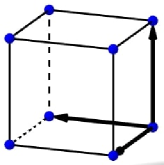
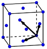
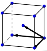
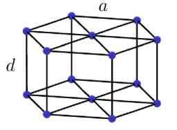
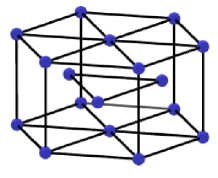
Figure 1. Main configurations of $\widetilde{\mathcal{L}_{3}}$: the SC lattice $\mathbb{Z}^{3}$ (up left), the FCC lattice $\mathsf{D}_{3}$ (up middle), the BCC lattice $\mathsf{D}_{3}^{*}$ (up right), the SH lattice $\mathsf{A_{f}}(\Delta)$ (down left), the anisotropy parameter $\Delta=d/a$, and the HCP lattice $\mathsf{A3}$ (down right).

1.3. Method

Whereas different rigorous techniques exist for studying lattice energies in dimension $d=2$ (see e.g. [53, 2, 5, 8, 10]), where $\dim\mathcal{L}_{2}=3$ and $\dim\mathcal{L}_{2}(V)=2$ for all $V>0$, the situation in dimension $d=3$ is much more complicated. Indeed the so-called fundamental domain containing only one copy of each lattice (up to dilation, isometry and symmetry) is $5$-dimensional for $\mathcal{L}_{3}(1)$ and has a complicated shape (see e.g. Terras [67]). Very few rigorous results have been proven in dimension 3. Let us recall as an example the computer-assisted proof of Sarnak and Strömbergsson [63] where the FCC lattice is shown to be minimal for the height of the flat torus (i.e. the derivative of $s\mapsto\zeta_{L}(s)$ at $s=0$).

In our work, we parametrize any lattice $L\in\mathcal{L}_{3}$ by $6$ real numbers $(u,v,x,y,z,V)$ where $V$ is the covolume of $L$ and, following [4],

$$L:=V^{\frac{1}{3}}\left[\mathbb{Z}u_{1}\oplus\mathbb{Z}u_{2}\oplus\mathbb{Z}u_{3}\right],$$

$$u_{1}=2^{\frac{1}{6}}\left(\frac{1}{\sqrt{u}},0,0\right),\quad u_{2}=2^{\frac{1}{6}}\left(\frac{x}{\sqrt{u}},\frac{v}{\sqrt{u}},0\right),\quad u_{3}=2^{\frac{1}{6}}\left(\frac{y}{\sqrt{u}},\frac{vz}{\sqrt{u}},\frac{u}{v\sqrt{2}}\right).$$

This parametrization appears to be the same as in [63, Eq. (27)] where $(t_{12},t_{13},t_{23})=(x,y,z)$, $y_{1}=v^{-2}$ and $y_{2}=2u^{-3}v^{4}$. We therefore use the corresponding three-dimensional Grenier’s fundamental domain shifted by one half in order to have only one copy of the unit density FCC point in it, i.e. $(u,v,x,y,z)\in\mathcal{G}_{3}$ defined by the following 9 inequalities:

1. $1\leq(1+x-y)^{2}+v^{2}\left((1-z)^{2}+\frac{u^{3}}{2v^{4}}\right)$

2. $1\leq(x-y)^{2}+v^{2}\left((1-z)^{2}+\frac{u^{3}}{2v^{4}}\right)$

3. $1\leq x^{2}+v^{2}$

4. $1\leq y^{2}+v^{2}\left(z^{2}+\frac{u^{3}}{2v^{4}}\right)$

5. $1\leq(y-1)^{2}+v^{2}\left(z^{2}+\frac{u^{3}}{2v^{4}}\right)$

6. $1\leq z^{2}+\frac{u^{3}}{2v^{4}}$

7. $0\leq x\leq\frac{1}{2}$, $0\leq y\leq 1$, $0\leq z\leq\frac{1}{2}$.

Our goal is then to investigate the minimizers of the following type of energy per point

$$E_{f}[L]:=\frac{1}{2}\sideset{}{{}^{\prime}}{\sum}_{p\in L}f(|p|^{2})=\frac{1}{2}\sideset{}{{}^{\prime}}{\sum}_{j,k,l}f\left(\frac{2^{\frac{1}{3}}V^{\frac{2}{3}}}{u}\left[(j+xk+yl)^{2}+v^{2}(k+zl)^{2}+\frac{u^{3}}{2v^{2}}l^{2}\right]\right),$$

when $(u,v,x,y,z)\in\mathcal{G}_{3}$, $V>0$ and $f(r)\in\{r^{-\frac{s}{2}},ar^{-\frac{n}{2}}-br^{-\frac{m}{2}}\}$. Notice that when our potential $f$ is not summable (i.e. when $m,n,s\leq 3$), we have used the analytic continuation of the Epstein zeta function (see e.g. [31]), but the corresponding expression can always be written in terms of energies of type $E_{f}$.

To compute numerically the minimizers, we have used the optimization tool FindMinimum in Mathematica, which includes ConjugateGradient, PrincipalAxis, LevenbergMarquardt, Newton, QuasiNewton, InteriorPoint, and LinearProgramming methods. It has to be noticed that, as in [63], we can systematically restrict our study to a compact domain of $\mathcal{G}_{3}$ since our energy diverges or goes to zero as the parameters $(u,v)$ go to infinity (see also [7] for such example in two dimensions).

When $L\in\{\mathbb{Z}^{3},\mathsf{D}_{3},\mathsf{D}_{3}^{*},\mathsf{A_{f}}(\Delta),\mathsf{A3}\}$, the exact formulas of $E_{f}[L]$ and their analytic continuations can be found in Section 4. Also, since the shape (i.e. its class up to dilation and isometry) of the global minimizer of $E_{n,m}^{\rm{LJ}}$ is independent of $(a,b)$ (see [13]), we have decided to choose $a=\frac{m}{n-m}$ and $b=\frac{n}{n-m}$ as it is usually done in the Physics literature. Therefore, our Lennard-Jones type energy will be, for any lattice $L$,

$$E^{\rm LJ}_{n,m}[L]=\frac{m}{n-m}\zeta_{L}(n)-\frac{n}{n-m}\zeta_{L}(m).$$ (1.8)

Plan of the paper. Section 2 and 3 are respectively devoted to investigate the lattice ground states for Riesz and Lennard-Jones type energies. The exact formulas used to compute our energies are stated in Section 4.

2. Minimizers of the Riesz energy

In this part, we investigate the minimizers of the Epstein zeta function $L\mapsto\zeta_{L}(s)$ in $\mathcal{L}_{3}(1)$ or $\widetilde{\mathcal{L}_{3}}(1)$ and for any $s\in\mathbb{R}$. The formulas we are using are available in Section 4. It is indeed enough to consider the $V=1$ case because the Epstein zeta function is homogeneous, i.e.

$$\zeta_{V^{\frac{1}{3}}L}(s)=V^{-\frac{s}{3}}\zeta_{L}(s),\quad\forall V>0,\quad\forall s\in\mathbb{R}.$$ (2.1)

It is already known (see [33, 39]) that $\mathsf{D}_{3}$ and $\mathsf{D}_{3}^{*}$ are both local minimizers of $L\mapsto\zeta_{L}(s)$ in $\mathcal{L}_{3}(1)$ for all $s>0$. Except of the minimality result of $\mathsf{D}_{3}$ for the height of the flat torus $L\mapsto\zeta_{L}^{\prime}(0)$ in [63] (and its very recent application [59] to the optimality of $\mathsf{D}_{3}^{*}$ for diblock copolymer molecular systems) as well as the optimality of $\mathbb{Z}^{d}$ among $d$-dimensional orthorhombic lattices following from Montgomery’s work [53], we are not aware of any other global optimality results in dimension $d=3$ for the Epstein zeta function.

First, we have re-checked the following well-known observations (see [63]):

• for all $0<s<\frac{3}{2}$, $\mathsf{D}_{3}^{*}$ is the unique minimizer of $L\mapsto\zeta_{L}(s)$ in $\mathcal{L}_{3}(1)$;

• for all $s>\frac{3}{2}$, $\mathsf{D}_{3}$ is the unique minimizer of $L\mapsto\zeta_{L}(s)$ in $\mathcal{L}_{3}(1)$.

Furthermore, it is easy to show (see e.g. (4.22) applied to $s=3/2$) that $\zeta_{\mathsf{D}_{3}}\left(\frac{3}{2}\right)=\zeta_{\mathsf{D}_{3}^{*}}\left(\frac{3}{2}\right)$.

Minimization for $0<s<3$.

Here we use the analytic continuation with respect to $s$ of the Epstein zeta function. The energies of $\mathsf{D}_{3}$ and $\mathsf{D}_{3}^{*}$ have close values, hence we plot their difference in Figure 2. It vanishes for $s\to 0^{+}$ as $\zeta_{L}(s)\to-1/2$ for any lattice $L$ and it remains finite for $s\to 3^{-}$ by the general Kronecker’s Limit Formula [20, Thm. 2.2]. The latter value was calculated semi-analytically. We can see that $\zeta_{\mathsf{D}_{3}}(s)-\zeta_{\mathsf{D}_{3}^{*}}(s)$ is positive for $0<s<3/2$ and negative otherwise, as expected.

Figure 2. Plot of $s\mapsto\zeta_{\mathsf{D}_{3}}(s)-\zeta_{\mathsf{D}_{3}^{*}}(s)$ for $s\in[0,3]$.

Minimization for $s>3$.

Recall that for large $s$ the FCC and HCP lattices could compete as they are closed packed lattices so that they should have common asymptotes. The large $s$ expansions can be deduced from summation formulas of the type (4.26) by inspection. For the FCC lattice we get

$$\zeta_{\mathsf{D}_{3}}(s)\approx\frac{1}{2^{s/6}}\left[6+\frac{3}{2^{s/2}}+\frac{12}{3^{s/2}}+\frac{6}{2^{s}}+\ldots\right]$$ (2.2)

whereas for the HCP one

$$\zeta_{\mathsf{A3}}(s)\approx\frac{1}{2^{s/6}}\left[6+\frac{3}{2^{s/2}}+\frac{1}{\big{(}\frac{8}{3}\big{)}^{s/2}}+\frac{9}{3^{s/2}}+\ldots\right].$$ (2.3)

We can see that both the leading and sub-leading terms are equal and for large enough $s$ the third term decides that $\zeta_{\mathsf{D}_{3}}(s)<\zeta_{\mathsf{A3}}(s)$ as $3>8/3$. This still does not mean that HCP could not prevail for some medium values of $s$. The values of the third term become equal for $s\approx 21$. Hence we performed high precision numerical calculations presented in Figure 3.

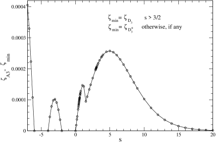
Figure 3. Plot of $s\mapsto\zeta_{\mathsf{A3}}(s)-\min\{\zeta_{\mathsf{D}_{3}}(s),\zeta_{\mathsf{D}_{3}^{*}}(s)\}$ for $s\in[-7,20]$.

We can see that $\zeta_{\mathsf{A3}}(s)-\zeta_{\mathsf{D}_{3}}(s)$ remains positive for all $s>3/2$, as expected. The apparent non-analyticity at $s=3/2$ is given by the fact, that we subtract another function for $s<3/2$, namely $\zeta_{\mathsf{A3}}(s)-\zeta_{\mathsf{D}_{3}^{*}}(s)$, in order to show that $\mathsf{A3}$ does not become the minimizer at any $s$. Note that the plotted difference is smooth at $s\to 3$ although both $\zeta_{\mathsf{A3}}(s)$ and $\zeta_{\mathsf{D}_{3}}(s)$ diverge.

Minimization for $s<0$.

Here we use the analytic continuation with respect to $s$ of the Epstein zeta function. At first let us state that this region is physically not very reasonable, but we can study it nevertheless. As recalled in the introduction, its minimum value is related to the Jellium problem with Riesz interaction. All analytically continued energies include the factor $1/\Gamma(s/2)$. It tends to zero at $s/2\to 0,-1,-2,$ etc. The case $s\to 0$ should be omitted, as we already mentioned that, for all lattice $L$, $\zeta_{L}(s)\to-1/2$ in the sense of limit. All the other zeros are present; in the 1D case of Riemann’s zeta function they are called trivial zeros. The energies are analytical functions thus they change signs at these points; they become negative at $-2<s<0$, $-6<s<-4$, etc., and they are positive otherwise. The negativity of energies gives rise to extremely low possible values of energies, say for simple hexagonal lattice $\mathsf{A_{f}}$ with very large anisotropy parameter $\Delta=d/a$ (where $a$ is the lattice constant and $d$ is the inter-layer distance), or for very dilated orthorhombic lattices, and it has no lower bound. In other words for $-4n-2<s<-4n$ with $n=0,1,2,\ldots$ there is no lattice the single minimizer as the energies diverge $\zeta_{\mathsf{A_{f}}}(s)\to-\infty$ for $\Delta\to\infty$. Finally for intervals $-4n<s<-4n+2$ with $n=1,2,\ldots$ where the energies are positive we have the minimizer and it is the BCC lattice. This was used in the left part of Figure 3 as well as in Figure 4. One could plot those differences also in the intervals where they are negative and see continuous oscillating functions, but non of the lattices represents the minimizer there.

Figure 4. Plot of $s\mapsto\zeta_{\mathsf{D}_{3}}(s)-\zeta_{\mathsf{D}_{3}^{*}}(s)$ when $s\in[-11,0)$.

Concluding, for real $s\neq 3$ we still have two lattices that become minimizers at some intervals of $s$. There is no minimizer for $-4n-2<s<-4n$ with $n=0,1,2,\ldots$; the FCC lattice minimizes the Riesz energy for $s>3/2$ and BCC otherwise. The result for negative $s$ is new.

According to our numerical investigation, we can therefore write the following conjecture for the Riesz energy, completing the one of Sarnak and Strömbergsson in [63].

Conjecture 2.1.

We have the following minimizers in $\widetilde{\mathcal{L}_{3}}(1)$ for the Epstein zeta function $L\mapsto\zeta_{L}(s)$:

• for all $n\in\mathbb{N}$ and all $s\in(-4n,-4n+2)$, the unique minimizer is $\mathsf{D}_{3}^{*}$;

• for all $n\in\mathbb{N}\cup\{0\}$ and all $s\in(-4n-2,-4n)$, the lattice energy has no minimizer;

• for all $s\in(0,3/2)$, the unique minimizer is $\mathsf{D}_{3}^{*}$;

• for all $s>3/2$, the unique minimizer is $\mathsf{D}_{3}$.

3. Minimizers of the Lennard-Jones type energy

In this section, we numerically investigate the minimizers of the Lennard-Jones type energy $L\mapsto E_{n,m}^{\rm LJ}[L]$ in $\mathcal{L}_{3}$ or $\widetilde{\mathcal{L}_{3}}$ (i.e. without any constraint on the density) and $\mathcal{L}_{3}(V)$ or $\widetilde{\mathcal{L}_{3}}(V)$, $V>0$ (i.e. at fixed density). Using the homogeneity (2.1) of the Epstein zeta function, we recall that, for all $V>0$ and all $L\in\widetilde{\mathcal{L}_{3}}(1)$,

$$E_{n,m}^{\rm{LJ}}[V^{\frac{1}{3}}L]=\frac{m}{n-m}\frac{\zeta_{L}(n)}{V^{\frac{n}{3}}}-\frac{n}{n-m}\frac{\zeta_{L}(m)}{V^{\frac{m}{3}}}.$$

For making our plots, we therefore use again the formulas derived in Section 4 evaluated by using the symbolic computer language Mathematica with precision of 16 decimal digits.

Again, only local minimality results for $E_{n,m}^{\rm LJ}$ are known. In particular, $V^{\frac{1}{3}}\mathsf{D}_{3}$ and $V^{\frac{1}{3}}\mathsf{D}_{3}^{*}$ have been shown in [4] to be locally minimal for $E_{n,m}^{\rm LJ}$ in $\mathcal{L}_{3}(V)$ for all fixed $V\in(0,V_{0})$ where $V_{0}=V_{0}(n,m)$ is explicit and sharp. Furthermore, the SC lattice $V^{\frac{1}{3}}\mathbb{Z}^{3}$ is also showed in the same work to be locally minimal in a certain interval $(V_{1},V_{2})$ of volume. The only other known results are the asymptotic global optimality of a FCC lattice for large $s$ (see [13]) and some other minimality results among lattices with prescribed number of nearest-neighbors in [6].

The values of the Lennard-Jones exponents $m$ and $n$, constrained by $m<n$, can lie in three distinct regions: $(3,\infty)$, $[0,3)$ and $(-\infty,0)$. While the lattice sums are convergent in the region $(3,\infty)$, they diverge (but still individual terms go asymptotically to zero) in the “critical” strip $[0,3)$ and they diverge (as well as individual terms diverge asymptotically) on the half-line $(-\infty,0)$. In this paper, we consider only such cases when both Lennard-Jones exponents $m$ and $n$ lie in the same region.

3.1. $3<m<n$

Minimization in $\mathcal{L}_{3}$ and $\widetilde{\mathcal{L}_{3}}$. Using dimension reduction techniques developed in [13] for Lennard-Jones type energies, we investigate the minimum of $E_{n,m}^{\rm LJ}$ in $\mathcal{L}_{3}$. As already explained in [77], only two lattices appear to be global minimizers of this energy: the FCC lattice and the HCP structure (see Figure 5). It seems that a large (resp. narrow) well, i.e. when $n-m$ is small (resp. large) favors the FCC (resp. HCP) lattice as a ground state. It has to be noticed that, whatever $n$ and $m$ are, the global minimizer of $E_{n,m}^{\rm LJ}$ in $\mathcal{L}_{3}$ is a FCC lattice. This also supports the conjecture that we stated in [4].

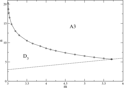
Figure 5. Global minimizer o $E_{n,m}^{\rm{LJ}}$ in $\widetilde{\mathcal{L}_{3}}$ with respect to $(n,m)$. The dash line corresponds to $m=n$. The phase diagram for the minimization problem on $\mathcal{L}_{3}$ is obtained by replacing the HCP phase by a FCC one.

Minimization in $\mathcal{L}_{3}(V)$ and $\widetilde{\mathcal{L}_{3}}(V)$. For the problem of minimizing $E_{n,m}^{\rm LJ}$ at fixed density, we have plotted in Figure 6 the phase diagram of $(n,V)\mapsto\mathop{\rm argmin}\nolimits_{L\in\mathcal{L}_{3}(V)}E_{n,m}^{\rm LJ}[L]$ where $m\in\{4,5,6\}$. We observe that there are only three kinds of minimizers in $\widetilde{\mathcal{L}_{3}}(V)$: the FCC lattice $V^{\frac{1}{3}}\mathsf{D}_{3}$, the Simple Hexagonal lattice $V^{\frac{1}{3}}\mathsf{A_{f}}(\Delta(V))$ and the HCP structure $V^{\frac{1}{3}}\mathsf{A3}$. More precisely, there exist $V_{n,m},V_{n,m}^{\prime}>0$ such that:

• for all $V\in(0,V_{n,m})$, $V^{\frac{1}{3}}\mathsf{D}_{3}$ is the unique minimizer of $E_{n,m}^{\rm LJ}$ in $\widetilde{\mathcal{L}_{3}}(V)$;

• for all $V\in(V_{n,m},V_{n,m}^{\prime})$, $V^{\frac{1}{3}}\mathsf{A3}$ is the unique minimizer of $E_{n,m}^{\rm LJ}$ in $\widetilde{\mathcal{L}_{3}}(V)$;

• for all $V>V_{n,m}^{\prime}$, $V^{\frac{1}{3}}\mathsf{A_{f}}(\Delta)$ is the unique minimizer of $E_{n,m}^{\rm LJ}$ in $\widetilde{\mathcal{L}_{3}}(V)$ for some $\Delta=\Delta(V)$, where the behavior of $\Delta(V)$ is depicted in Figure 7 for $n=12$ and $m\in\{4,5,6\}$.

If we minimize $E_{n,m}^{\rm LJ}$ only in $\mathcal{L}_{3}(V)$, the HCP phase is replaced by a FCC one in such a way that

• for all $V\in(0,V_{n,m}^{\prime})$, $V^{\frac{1}{3}}\mathsf{D}_{3}$ is the unique minimizer of $E_{n,m}^{\rm LJ}$ in $\mathcal{L}_{3}(V)$;

• for all $V>V_{n,m}^{\prime}$, $V^{\frac{1}{3}}\mathsf{A_{f}}(\Delta)$ is the unique minimizer of $E_{n,m}^{\rm LJ}$ in $\mathcal{L}_{3}(V)$ for some $\Delta=\Delta(V)$ as depicted in Figure 7.

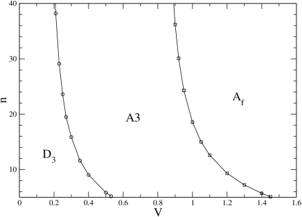
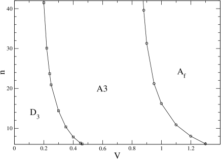
Figure 6. Phase diagram of the minimizer of $E_{n,m}^{\rm{LJ}}$ in $\widetilde{\mathcal{L}_{3}}(V)$ for $m=4$ (up left) and $m=5$ (up right) and $m=6$ (down), $n$ varying. The phase diagram for the minimization problem on $\mathcal{L}_{3}(V)$ is roughly obtained by replacing the HCP phase by a FCC one.

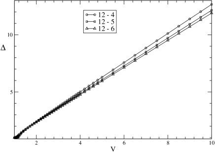
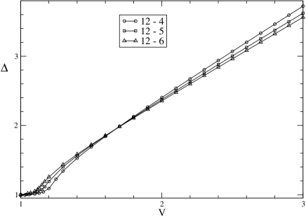
Figure 7. Simple Hexagonal phase. Plot of $V\mapsto\mathop{\rm argmin}\nolimits_{\Delta}E_{n,m}^{\rm{LJ}}[V^{\frac{1}{3}}\mathsf{A}_{f}(\Delta)]$ for $(n,m)\in\{(12,m):m=4,5,6\}$.

In [4], the interval of volumes $V$ where the SC lattice is locally minimal for $E_{n,m}^{\rm{LJ}}$ in $\mathcal{L}_{3}(V)$ has been derived. Here we have observed that a family of SH lattices have lower energy than the SC one. This is new compared to the two-dimensional case where the square lattice, that has been shown in [3] to be locally minimal in some interval of volume, is also observed to be minimal in $\mathcal{L}_{2}(V)$ in the same interval. Furthermore, our numerical findings concerning the global minimizer of $E_{n,m}^{\rm{LJ}}$ in $\mathcal{L}_{3}$ support [4] and confirm [77].

3.2. $0<m<n<3$

Let us now consider that the Lennard-Jones exponents $n$ and $m$ lie in the critical strip and fix $m=1$. It turns out that for any value of $1<n<3$ the ${\rm A_{f}}$ lattice with the extreme value of the anisotropy parameter $\Delta_{\rm opt}\to\infty$ yields the lowest possible energy per site $E_{\rm A_{f}}\to-\infty$. In order to get non-trivial results at fixed density, we will restrict ourselves to rigid lattices: ${\mathbb{Z}^{3}}$, ${\rm D_{3}^{*}}$, ${\rm D_{3}}$ and ${\rm A3}$. One can see in the inset of Fig. 8 that for small values of $n$ close to 1 and very small elementary cell volume $V$ up to 0.01, the ${\rm D_{3}^{*}}$ lattice prevails. Note that the phase boundary between ${\rm D_{3}^{*}}$ and ${\rm D_{3}}$ lattices ends at $n=1.5$; this is due to the fact that for an infinitesimal $V$ the $n$ term dominates in the Lennard-Jones energy and it holds that $E_{\rm D_{3}^{*}}(3/2)=E_{\rm D_{3}}(3/2)$ for the Riesz interaction at $s=3/2$. For larger values of $n$ and $V$, there is a competition between the ${\rm D_{3}}$ and ${\rm A3}$ lattices as minimizers of the energy. The boundary between the two lattices runs within the interval approximately $1.28<V<2.09$. There is numerical evidence that if we chose the exponent $m\geq 1.5$, the ${\rm D_{3}^{*}}$ lattice would disappear from the phase diagram.

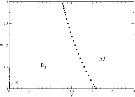
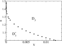
Figure 8. Phase diagram for the minimum Lennard-Jones energy for the exponents $m=1$ and $1<n<3$ at fixed density $1/V$.

3.3. $-2<m<n<0$

Within this interval of the exponents, the ${\rm D_{3}^{*}}$ lattice becomes the minimizer of the enegy for any value of $V$. The ${\rm A_{f}}$ lattice has its (finite) minimum energy for a finite value of $\Delta_{\rm opt}$, but its energy is not low enough to become the global minimizer.

3.4. $-4<m<n<-2$

Now both ${\rm D_{3}^{*}}$ and ${\rm A_{f}}$ lattices are candidates for global minimizers, the latter lattice with a finite parameter $0.6<\Delta_{opt}<0.9$ for the presently calculated data. The typical phase diagram for the Lennard-Jones exponents $m=-3.5$ and $-3.5<n<-2$ is plotted in Fig. 9. The phase curve between the ${\rm D_{3}^{*}}$ and ${\rm A_{f}}$ lattices approaches to $n=-3.5$ at asymptotically large $V\to\infty$. Analogous phase diagrams appear in intervals $-6<m<n<-4$, etc.

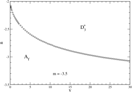
Figure 9. Phase diagram of the lowest Lennard-Jones energy for the exponents $m=-3.5$ and $-3.5<n<-2$.

According to our numerical study, we can write the following conjecture for the ground state of the Lennard-Jones type energy.

Conjecture 3.1.

Concerning the global minimizer of $E_{n,m}^{\textnormal{LJ}}$, we have:

• for $3<m<n$, then we have two cases:

  1. in $\mathcal{L}_{3}$, the unique minimizer of $E_{n,m}^{\textnormal{LJ}}$ is $\mathsf{D}_{3}$, up to rescaling.

  2. in $\widetilde{\mathcal{L}_{3}}$, there exists $m_{0}\approx 5.7$ such that,

     • if $m<m_{0}$, then there exists $n_{m}$ such that if $n<n_{m}$ (resp. $n>n_{m}$), the unique minimizer of $E_{n,m}^{\textnormal{LJ}}$ is $\mathsf{D}_{3}$ (resp. $\mathsf{A}_{3}$), up to rescaling.

     • if $m>m_{0}$, then the unique minimizer of $E_{n,m}^{\textnormal{LJ}}$ is $\mathsf{A}_{3}$.

• for $0<m<n<3$, $E_{n,m}^{\textnormal{LJ}}$ does not have any minimizer at fixed density.

• for all $k\in\mathbb{N}\cup\{0\}$, for all $-4k-2<m<n<-4k$, the unique minimizer of $E_{n,m}^{\textnormal{LJ}}$ in $\widetilde{\mathcal{L}_{3}}$ is $\mathsf{D}_{3}^{*}$, up to rescaling;

• for all $k\in\mathbb{N}$, for all $-4k<m<n<-4k+2$, $\mathsf{D}_{3}^{*}$ and $\mathsf{A_{f}}$ are both minimizers, up to rescaling, of $E_{n,m}^{\textnormal{LJ}}$ in $\widetilde{\mathcal{L}_{3}}$.

4. Explicit formulas for three-dimensional Epstein zeta functions

This section is devoted to the construction of explicit formulas for Epstein zeta functions associated to the three-dimensional lattices considered in the present paper. We start with converging sums, i.e., the parameter $s$ is larger than dimension 3, and express them as integrals over powers of Jacobi elliptic functions. Then using specific tricks with elliptic functions these integrals are rewritten into the ones which represent an analytic continuation of Epstein zeta functions to the whole complex plane except for $s=3$.

4.1. Simple cubic lattice

Let particles be localized at sites of the SC lattice with spacing $a$. In this paper, we compare the energy per particle for various 3D lattice structures at a fixed density of particles, say the unit one. The particle density associated with the SC lattice, given by $\rho=1/a^{3}$, is equal to one when $a=1$. Particles interact pairwisely by the Riesz potential $1/r^{s}$ where $r=|{\bf r}|$ is the distance between two particles and $s$ is a complex number. The energy per particle is given by the Epstein zeta function associated with the SC lattice

$$\zeta_{\mathbb{Z}^{3}}(s)=\frac{1}{2}\sum_{(j,k,l)\neq(0,0,0)}\frac{1}{(j^{2}+k^{2}+l^{2})^{s/2}},$$ (4.1)

where the prefactor $1/2$ is due to the fact that every energy is shared by two particles and the sum converges only if the real part of $s$ $\Re(s)>3$. Using the $\Gamma$-identity

$$\frac{1}{r^{s}}=\frac{1}{(r^{2})^{s/2}}=\frac{1}{\Gamma(s/2)}\int_{0}^{\infty}{\rm d}t\,t^{\frac{s}{2}-1}{\rm e}^{-r^{2}t},$$ (4.2)

the expression (4.1) can be rewritten as

$$\zeta_{\mathbb{Z}^{3}}(s) = \frac{1}{2\Gamma(s/2)}\int_{0}^{\infty}\frac{{\rm d}t}{t}t^{s/2}\left[\sum_{j,k,l=-\infty}^{\infty}{\rm e}^{-(j^{2}+k^{2}+l^{2})t}-1\right]$$ (4.3)

$$= \frac{1}{2\Gamma(s/2)}\int_{0}^{\infty}\frac{{\rm d}t}{t}t^{s/2}\left[\theta_{3}^{3}\left({\rm e}^{-t}\right)-1\right]$$

$$= \frac{\pi^{s/2}}{2\Gamma(s/2)}\int_{0}^{\infty}\frac{{\rm d}t}{t}t^{s/2}\left[\theta_{3}^{3}\left({\rm e}^{-\pi t}\right)-1\right],$$

where the Jacobi elliptic function with zero argument $\vartheta_{3}(0,q)\equiv\theta_{3}(q)=\sum_{j=-\infty}^{\infty}q^{j^{2}}$ [38] was introduced for $q=e^{i\pi\tau}$, $\Im(\tau)>0$. Notice that (4.3) can be obtained from the Mellin transform of the Jacobi theta function (see e.g. [43] and [66, Sec. 1.4.2]). With regard to the definition of $\theta_{3}(q)$, it holds that $\theta_{3}\left({\rm e}^{-\pi t}\right)\sim_{t\to\infty}1+2{\rm e}^{-\pi t}+\cdots$ and the integral in (4.3) converges at large $t$ for any $s$. Using the Poisson summation formula

$$\sum_{j=-\infty}^{\infty}{\rm e}^{-(j+\phi)^{2}\pi t}=\frac{1}{\sqrt{t}}\sum_{j=-\infty}^{\infty}{\rm e}^{2\pi{\rm i}j\phi}{\rm e}^{-(\pi j^{2})/t}$$ (4.4)

it can be shown that

$$\theta_{3}\left({\rm e}^{-\pi t}\right)\mathop{\sim}_{t\to 0}\frac{1}{\sqrt{t}}\left(1+2{\rm e}^{-\pi/t}+\cdots\right).$$ (4.5)

The function under integration in (4.3) behaves like $t^{\frac{s-3}{2}-1}$ for $t\to 0$, so the real part of $s$ must be greater than 3 as was expected.

To derive an analytic continuation of (4.3) to the complex-$s$ plane, we follow the derivation presented in Ref. [70] for $d$-dimensional hypercubic lattices. In the integral on the rhs of (4.3), we split the integration over $t$ into intervals $[0,1]$ and $[1,\infty]$. In the second integral over $t\in[1,\infty]$, one applies the equality

$$\theta_{3}(e^{-\pi t})=\frac{1}{\sqrt{t}}\theta_{3}\left({\rm e}^{-\pi/t}\right)$$ (4.6)

which follows from (4.4) and substitutes $t=1/t^{\prime}$ to get

$$\int_{1}^{\infty}\frac{{\rm d}t}{t}t^{s/2}\left[\theta_{3}^{3}\left({\rm e}^{-\pi t}\right)-1\right]=\int_{0}^{1}\frac{{\rm d}t^{\prime}}{t^{\prime}}{t^{\prime}}^{(3-s)/2}\left[\theta_{3}^{3}\left({\rm e}^{-\pi t^{\prime}}\right)-{t^{\prime}}^{-3/2}\right].$$ (4.7)

As concerns the first integral over $t\in[0,1]$, to subtract the singularity of $\theta_{3}^{3}\left({\rm e}^{-\pi t}\right)\sim t^{-3/2}$ as $t\to 0$ one adds the vanishing contribution $-t^{-3/2}+t^{-3/2}$ and integrates out the remaining terms proportional to $t^{-3/2}-1$, with the result

$$\frac{\Gamma{(s/2)}}{\pi^{s/2}}\zeta_{\mathbb{Z}^{3}}(s)=-\frac{1}{s}-\frac{1}{3-s}+\int_{0}^{1}\frac{{\rm d}t}{2t}\ \left[t^{s/2}+t^{(3-s)/2}\right]\left[\theta_{3}^{3}\left({\rm e}^{-\pi t}\right)-\frac{1}{t^{3/2}}\right].$$ (4.8)

The difference in the square bracket is proportional to $t^{-3/2}e^{-\pi/t}$ for $t\to 0$ and hence the formula (4.8) converges for all complex $s$, except for the singular point $s=3$. The limit $s\to 0$ is not problematic since the singularity $-1/s$ on the rhs of (4.8) has a counterpart $\Gamma(s/2)\sim 2/s$ on the lhs, so that $\zeta_{\mathbb{Z}^{3}}(0)=-1/2$. The numerical evaluation of $\zeta_{\mathbb{Z}^{3}}(s)$ by using (4.8) at one point $s$ takes around 5 seconds of CPU time on a standard PC, the achieved accuracy is around 29 decimal digits. Similar characteristics occur in the numerical evaluation of all Epstein functions studied below, except for the HCP structure given by the lattice sum for which the calculation of the Epstein function takes around 1 minute.

It is known that the transformation $s\to 3-s$ connects the lattice sums of dual (reciprocal) lattice structures [18]. The SC lattice is self-dual. The rhs of (4.8) is invariant with respect to this transformation, hence it holds that

$$\zeta_{\mathbb{Z}^{3}}(s)=\frac{\pi^{s-3/2}\,\Gamma\left(\frac{3-s}{2}\right)}{\Gamma\left(\frac{s}{2}\right)}\zeta_{\mathbb{Z}^{3}}(3-s).$$ (4.9)

4.2. Body centered cubic lattice

The BCC lattice is composed of two SC lattices, shifted with respect to one another by half-period along each of the three coordinates. There are two particles per elementary cube of side $a_{\rm BCC}$, i.e., $\rho=2/a^{3}_{\rm BCC}=1$ which implies that the unit density corresponds to $a_{\rm BCC}=2^{1/3}$. Consequently,

$$\zeta_{\mathsf{D}_{3}^{*}}(s)=\frac{1}{2^{s/3}}\left[\zeta_{\mathbb{Z}^{3}}(s)+\psi(1/2,1/2,1/2;s)\right],$$ (4.10)

where

$$\psi(x_{1},x_{2},x_{3};s) = \frac{1}{2}\sum_{j,k,l=-\infty}^{\infty}\frac{1}{[(j-x_{1})^{2}+(k-x_{2})^{2}+(l-x_{3})^{2}]^{s/2}}$$ (4.11)

$$= \frac{1}{2\Gamma(s/2)}\int_{0}^{\infty}\frac{{\rm d}t}{t}t^{s/2}\sum_{j,k,l=-\infty}^{\infty}{\rm e}^{-[(j-x_{1})^{2}+(k-x_{2})^{2}+(l-x_{3})^{2}]t}$$

is a sum over a lattice shifted with respect to the original cubic one. Introducing another Jacobi elliptic function $\theta_{2}(q)=\sum_{j=-\infty}^{\infty}q^{(j-\frac{1}{2})^{2}}$, defined for $q=e^{i\pi\tau}$, $\Im(\tau)>0$, the BCC energy is expressible as

$$\zeta_{\mathsf{D}_{3}^{*}}(s)=\frac{1}{2^{s/3}}\left[\zeta_{\mathbb{Z}^{3}}(s)+\frac{\pi^{s/2}}{2\Gamma(s/2)}\int_{0}^{\infty}\frac{{\rm d}t}{t}t^{s/2}\theta_{2}^{3}({\rm e}^{-\pi t})\right].$$ (4.12)

In view of the Poisson summation formula (4.4), the Jacobi theta function $\theta_{4}(q)=\sum_{j=-\infty}^{\infty}(-1)^{j}q^{j^{2}}$ is “dual” to $\theta_{2}$ in the sense that

$$\theta_{2}\left({\rm e}^{-\pi t}\right)=\frac{1}{\sqrt{t}}\theta_{4}\left({\rm e}^{-\pi/t}\right).$$ (4.13)

Thus,

$$\theta_{2}\left({\rm e}^{-\pi t}\right)\mathop{\sim}_{t\to 0}\frac{1}{\sqrt{t}}\left(1-2{\rm e}^{-\pi/t}+\cdots\right)$$ (4.14)

and the integral in (4.12) converges at small $t$ if $\Re(s)>3$ as was expected.

To derive an analytic continuation of (4.12) we proceed in close analogy with the previous SC lattice. The integration on the rhs of (4.12) is split into intervals $[0,1]$ and $[1,\infty]$. The second integral over $t\in[1,\infty]$ can be transformed by using the relation (4.13) and the consequent substitution $t=1/t^{\prime}$ to

$$\int_{1}^{\infty}\frac{{\rm d}t}{t}t^{s/2}\theta_{2}^{3}({\rm e}^{-\pi t})=\int_{0}^{1}{\rm d}t^{\prime}\,{t^{\prime}}^{(1-s)/2}\theta_{4}^{3}({\rm e}^{-\pi t^{\prime}}).$$ (4.15)

The first integral over $t\in[0,1]$ is modified by adding the vanishing contribution $-t^{-3/2}+t^{-3/2}$; the term $-t^{-3/2}$ removes the singularity of $\theta_{2}^{3}({\rm e}^{-\pi t})$ as $t\to 0$ and the term $t^{-3/2}$ is integrated out. The final formula for the Epstein function associated with the BCC lattice reads as

$$\frac{2^{s/3}\Gamma(s/2)}{\pi^{s/2}}\zeta_{\mathsf{D}_{3}^{*}}(s) = \frac{\Gamma{(s/2)}}{\pi^{s/2}}\zeta_{\mathbb{Z}^{3}}(s)-\frac{1}{3-s}$$ (4.16)

$$+\int_{0}^{1}\frac{{\rm d}t}{2t}\left\{t^{s/2}\left[\theta_{2}^{3}\left({\rm e}^{-\pi t}\right)-\frac{1}{t^{3/2}}\right]+t^{(3-s)/2}\theta_{4}^{3}\left({\rm e}^{-\pi t}\right)\right\},$$

where $\zeta_{\mathbb{Z}^{3}}(s)$ is given by (4.8). Since

$$\theta_{4}\left({\rm e}^{-\pi t}\right)\mathop{\sim}_{t\to 0}\frac{1}{\sqrt{t}}{\rm e}^{-\pi/(4t)}+\cdots,$$ (4.17)

the integral in (4.16) converges for any complex $s$.

4.3. Face centered cubic lattice

There are four particles per elementary cube of side $a_{\rm FCC}$. thus $\rho=4/a^{3}_{\rm FCC}=1$ which implies that $a_{\rm FCC}=2^{2/3}$. For $\Re(s)>3$, one gets

$$\zeta_{\mathsf{D}_{3}}(s) = \frac{1}{2^{2s/3}}\left[\zeta_{\mathbb{Z}^{3}}(s)+\psi\left(0,\frac{1}{2},\frac{1}{2};s\right)+\psi\left(\frac{1}{2},0,\frac{1}{2};s\right)+\psi\left(\frac{1}{2},\frac{1}{2},0;s\right)\right]$$ (4.18)

$$= \frac{1}{2^{2s/3}}\left[\zeta_{\mathbb{Z}^{3}}(s)+\frac{3\pi^{s/2}}{2\Gamma(\frac{s}{2})}\int_{0}^{\infty}\frac{{\rm d}t}{t}t^{s/2}\theta_{2}^{2}\left({\rm e}^{-\pi t}\right)\theta_{3}\left({\rm e}^{-\pi t}\right)\right].$$

Splitting the integration into the intervals $[0,1]$ and $[1,\infty]$ and using the equality

$$\int_{1}^{\infty}\frac{{\rm d}t}{t}t^{s/2}\theta_{2}^{2}\left({\rm e}^{-\pi t}\right)\theta_{3}\left({\rm e}^{-\pi t}\right)=\int_{0}^{1}{\rm d}t\,t^{(1-s)/2}\theta_{4}^{2}\left({\rm e}^{-\pi t}\right)\theta_{3}\left({\rm e}^{-\pi t}\right),$$ (4.19)

the analytic continuation of (4.18) to the whole complex $s$-plane (except for the singular point $s=3$) takes the form

$$\frac{2^{2s/3}\Gamma(s/2)}{\pi^{s/2}}\zeta_{\mathsf{D}_{3}}(s) = \frac{\Gamma{(s/2)}}{\pi^{s/2}}\zeta_{\mathbb{Z}^{3}}(s)-\frac{3}{3-s}$$ (4.20)

$$+\frac{3}{2}\int_{0}^{1}\frac{{\rm d}t}{t}\Bigg{\{}t^{s/2}\left[\theta_{2}^{2}\left({\rm e}^{-\pi t}\right)\theta_{3}\left({\rm e}^{-\pi t}\right)-\frac{1}{t^{3/2}}\right]$$

$$+t^{(3-s)/2}\theta_{4}^{2}\left({\rm e}^{-\pi t}\right)\theta_{3}\left({\rm e}^{-\pi t}\right)\Bigg{\}}.$$

The FCC and BCC lattices is a pair of dual structures. Exploring theta-function identities [75]

$$\theta_{3}(q)=\theta_{3}(q^{4})+\theta_{2}(q^{4}),\qquad\theta_{4}(q)=\theta_{3}(q^{4})-\theta_{2}(q^{4})$$ (4.21)

in the representations (4.16) and (4.20) it can be shown after some algebra that

$$\zeta_{\mathsf{D}_{3}^{*}}(s)=\frac{\pi^{s-3/2}\,\Gamma\left(\frac{3-s}{2}\right)}{\Gamma\left(\frac{s}{2}\right)}\zeta_{\mathsf{D}_{3}}(3-s)$$ (4.22)

or, vice versa,

$$\zeta_{\mathsf{D}_{3}}(s)=\frac{\pi^{s-3/2}\,\Gamma\left(\frac{3-s}{2}\right)}{\Gamma\left(\frac{s}{2}\right)}\zeta_{\mathsf{D}_{3}^{*}}(3-s).$$ (4.23)

The turning point of these transformations is $s=3/2$ where $\zeta_{\mathsf{D}_{3}}(3/2)=\zeta_{\mathsf{D}_{3}^{*}}(3/2)$.

4.4. Simple hexagonal lattice

The SH lattice is composed of parallel planes composed of the 2D hexagonal lattice with spacing $a_{\rm SH}$, the distance between the nearest-neighbor planes is $d$; the dimensionless parameter $\Delta=d/a_{\rm SH}$. The 2D hexagonal lattice can be considered as the union of two rectangle lattices of sides $a_{\rm SH}$ and $\sqrt{3}a_{\rm SH}$, shifted with respect to one another by a half-period. Thus the sites of the SH lattice can be parameterized with respect to the reference point $(0,0,0)$ as follows: $a_{\rm SH}(j,\sqrt{3}k,\Delta l)$ with integers $j,k,l$ such that $(j,k,l)\neq(0,0,0)$ and $a_{\rm SH}\left[(j+\frac{1}{2}),\sqrt{3}(k+\frac{1}{2}),\Delta l\right]$ with integer $j,k,l$. There are two particles in the elementary rectangular parallelepiped of volume $\sqrt{3}a_{\rm SH}^{2}d$, so the unit density of particles corresponds to $2/\left(\sqrt{3}\Delta a_{\rm SH}^{3}\right)=1$. For $\Re(s)>3$, the energy per particle for the SH lattice is given by

$$\zeta_{\mathsf{A_{f}}(\Delta)}(s) = \frac{\pi^{s/2}}{2a_{\rm SH}^{s}\Gamma(s/2)}\int_{0}^{\infty}\frac{{\rm d}t}{t}t^{s/2}\Big{[}\theta_{3}\left({\rm e}^{-\pi t}\right)\theta_{3}\left({\rm e}^{-3\pi t}\right)\theta_{3}\left({\rm e}^{-\pi t\Delta^{2}}\right)$$ (4.24)

$$-1+\theta_{2}\left({\rm e}^{-\pi t}\right)\theta_{2}\left({\rm e}^{-3\pi t}\right)\theta_{3}\left({\rm e}^{-\pi t\Delta^{2}}\right)\Big{]}.$$

The analytic continuation to the whole complex $s$-plane (except for the point $s=3$) is obtained in the form

$$\left(\frac{2}{\sqrt{3}\Delta}\right)^{s/3}\frac{\Gamma(s/2)}{\pi^{s/2}}\zeta_{\mathsf{A_{f}}(\Delta)}(s) = -\frac{1}{s}-\frac{2}{\Delta\sqrt{3}(3-s)}$$

$$+\int_{0}^{1}\frac{{\rm d}t}{2t}\Bigg{\{}t^{s/2}\Big{[}\theta_{3}\left({\rm e}^{-\pi t}\right)\theta_{3}\left({\rm e}^{-3\pi t}\right)\theta_{3}\left({\rm e}^{-\pi t\Delta^{2}}\right)$$

$$+\theta_{2}\left({\rm e}^{-\pi t}\right)\theta_{2}\left({\rm e}^{-3\pi t}\right)\theta_{3}\left({\rm e}^{-\pi t\Delta^{2}}\right)-\frac{2}{\sqrt{3}\Delta t^{3/2}}\Big{]}$$

$$+\frac{t^{(3-s)/2}}{\sqrt{3}\Delta}\Big{[}\theta_{3}\left({\rm e}^{-\pi t}\right)\theta_{3}\left({\rm e}^{-\pi t/3}\right)\theta_{3}\left({\rm e}^{-\pi t/\Delta^{2}}\right)$$

$$-\frac{\sqrt{3}\Delta}{t^{3/2}}+\theta_{4}\left({\rm e}^{-\pi t}\right)\theta_{4}\left({\rm e}^{-\pi t/3}\right)\theta_{3}\left({\rm e}^{-\pi t/\Delta^{2}}\right)\Big{]}\Bigg{\}}.$$

4.5. Hexagonal close-packed lattice

For very large $s\to\infty$ the Riesz potential $1/r^{s}$ tends to infinity for $r<1$ and vanishes for $r>1$, i.e. it approaches the hard-sphere limit. For this case a close-packed structure becomes the minimizer. There are two such lattices in 3D, besides the FCC also the hexagonal close-packed (HCP) lattice with the same packing ratio. The two lattices have common first order asymptotic value of the Epstein zeta function – since they have the same non-zero shortest vectors – and it is relatively simple to derive how their difference behaves for large $s$, see the relations (2.2) and (2.3).

The HCP lattice is pictured in Fig. 1; the middle hexagonal layer is shifted by a half-period with respect to the top and bottom hexagonal lattices. Denoting by $a_{\rm HCP}$ the spacing of the one-layer hexagonal lattice, the distance between top and bottom hexagonal layers is given by $d=\Delta a_{\rm HCP}$ with $\Delta=\sqrt{8/3}$. As an elementary cell we take the rectangular parallelepiped with sides $a_{\rm HCP}$ and $\sqrt{3}a_{\rm HCP}$ on the top and bottom layers and the height $d$, its volume is given by $\sqrt{3}a_{\rm HCP}^{2}d=\sqrt{8}a_{\rm HCP}^{3}$. There are 8 particles on the top and bottom layers each shared by 8 elementary cells, 2 particles on the top and bottom layers each shared by 2 cells, 1 particle on the middle layer sitting in the cell interior and 2 particles on the middle layer sitting on the cell surface (each shared by 2 cells), i.e. altogether there are 4 particles per elementary cell. The density of particles $\rho=4/(\sqrt{8}a_{\rm HCP}^{3})$ equals to unity when $a_{\rm HCP}=2^{1/6}$.

Particle positions on the top and bottom layers can be parameterized with respect to the reference particle at the origin $(0,0,0)$ as follows: $a_{\rm HCP}(j,\sqrt{3}k,\Delta l)$ with integer $j,k,l$ such that $(j,k,l)\neq(0,0,0)$ and $a_{\rm HCP}\left[(j+\frac{1}{2}),\sqrt{3}(k+\frac{1}{2}),\Delta l\right]$ with integer $j,k,l$. It can be shown that particle positions on the middle layer can be parameterized as follows: $a_{\rm HCP}\left[j,\sqrt{3}(k+\frac{2}{3}),\Delta(l+\frac{1}{2})\right]$ and $a_{\rm HCP}\left[(j+\frac{1}{2}),\sqrt{3}(k+\frac{1}{6}),\Delta(l+\frac{1}{2})\right]$ with integer $j,k,l$. The energy per particle of HCP lattice for $\Re(s)>3$ thus reads as

$$\zeta_{\mathsf{A3}}(s) = \frac{1}{2^{s/6+1}}\Bigg{\{}\sum_{(j,k,l)\neq(0,0,0)}\frac{1}{(j^{2}+3k^{2}+\frac{8}{3}l^{2})^{s/2}}$$ (4.26)

$$+\sum_{j,k,l}\frac{1}{[(j+1/2)^{2}+3(k+1/2)^{2}+\frac{8}{3}l^{2}]^{s/2}}$$

$$+\sum_{j,k,l}\frac{1}{[j^{2}+3(k+2/3)^{2}+\frac{8}{3}(l+1/2)^{2}]^{s/2}}$$

$$+\sum_{j,k,l}\frac{1}{[(j+1/2)^{2}+3(k+1/6)^{2}+\frac{8}{3}(l+1/2)^{2}]^{s/2}}\Bigg{\}}.$$

To obtain an analytic continuation of the energy to the whole complex plane $s$, except for the point $s=3$, all sums over integers $j$ and $l$ can be transformed directly to Jacobi elliptic functions by using the above explained summation techniques. The transformation of the sums over integers $k$ with the shifts of $k$ by $1/6$ and $2/3$ is not so straightforward, but still they are expressible as series of products of Jacobi elliptic functions and the cos-functions. In particular, one gets

$$\frac{2^{s/6+1}\Gamma(s/2)}{\pi^{s/2}}\zeta_{\rm A3}(s)=\frac{4}{\sqrt{2}(s-3)}-\frac{2}{s}$$

$$+\int_{0}^{1}{\rm d}t\,t^{s/2-1}\left[\theta_{3}({\rm e}^{-\pi t})\theta_{3}({\rm e}^{-3\pi t})\theta_{3}({\rm e}^{-8\pi t/3})-\frac{1}{\sqrt{8}t^{3/2}}\right]$$

$$+\int_{0}^{1}{\rm d}t\,t^{(1-s)/2}\left[\frac{1}{\sqrt{8}}\theta_{3}({\rm e}^{-\pi t})\theta_{3}({\rm e}^{-\pi t/3})\theta_{3}({\rm e}^{-3\pi t/8})-\frac{1}{t^{3/2}}\right]$$

$$+\int_{0}^{1}{\rm d}t\,t^{s/2-1}\left[\theta_{2}({\rm e}^{-\pi t})\theta_{2}({\rm e}^{-3\pi t})\theta_{3}({\rm e}^{-8\pi t/3})-\frac{1}{\sqrt{8}t^{3/2}}\right]$$

$$+\frac{1}{\sqrt{8}}\int_{0}^{1}{\rm d}t\,t^{(1-s)/2}\theta_{4}({\rm e}^{-\pi t})\theta_{4}({\rm e}^{-\pi t/3})\theta_{3}({\rm e}^{-3\pi t/8})$$

$$+\int_{0}^{1}{\rm d}t\,\frac{t^{s/2-1}}{\sqrt{3t}}\left[\theta_{2}({\rm e}^{-\pi t})\theta_{2}({\rm e}^{-8\pi t/3})-\frac{1}{\sqrt{8/3}t}\right]$$

$$+2\int_{0}^{1}{\rm d}t\,\frac{t^{s/2-1}}{\sqrt{3t}}\theta_{2}({\rm e}^{-\pi t})\theta_{2}({\rm e}^{-8\pi t/3})\sum_{j=1}^{\infty}\cos\left(\frac{\pi j}{3}\right){\rm e}^{-\pi j^{2}/(3t)}$$

$$+\int_{0}^{1}{\rm d}t\,\frac{t^{(1-s)/2}}{\sqrt{8}}\theta_{4}({\rm e}^{-\pi t})\theta_{4}({\rm e}^{-8\pi t/3})\left[1+2\sum_{j=1}^{\infty}\cos\left(\frac{\pi j}{3}\right){\rm e}^{-\pi tj^{2}/3}\right]$$

$$+\int_{0}^{1}{\rm d}t\,\frac{t^{s/2-1}}{\sqrt{3t}}\left[\theta_{3}({\rm e}^{-\pi t})\theta_{2}({\rm e}^{-8\pi t/3})-\frac{1}{\sqrt{8/3}t}\right]$$

$$+2\int_{0}^{1}{\rm d}t\,\frac{t^{s/2-1}}{\sqrt{3t}}\theta_{3}({\rm e}^{-\pi t})\theta_{2}({\rm e}^{-8\pi t/3})\sum_{j=1}^{\infty}\cos\left(\frac{4\pi j}{3}\right){\rm e}^{-\pi j^{2}/(3t)}$$

$$+\int_{0}^{1}{\rm d}t\,\frac{t^{(1-s)/2}}{\sqrt{8}}\theta_{3}({\rm e}^{-\pi t})\theta_{4}({\rm e}^{-3\pi t/8})\left[1+2\sum_{j=1}^{\infty}\cos\left(\frac{4\pi j}{3}\right){\rm e}^{-\pi tj^{2}/3}\right].$$

(4.27)

Here, in the numerical computation of infinite sums over cosine functions one has to truncate the sums as follows $\sum_{j=1}^{K}$ where the upper cut $K=1,2,3,\ldots$ is a positive integer. It turns out that by increasing $K$ the convergence of the sums to the exact value $(K\to\infty)$ is extremely quick. In particular, by using the symbolic computer language Mathematica it was checked for any real value of $s$ that the $K=4$ energy is determined with precision of 12 decimal digits, for $K=5$ the precision is increased to 16 decimal digits and so on.

References

- [1] A. Abrikosov. The Magnetic Properties of Superconducting Alloys. Journal of Physics and Chemistry of Solids, 2:199–208, 1957.
- [2] L. Bétermin. Two-dimensional Theta Functions and Crystallization among Bravais Lattices. SIAM J. Math. Anal., 48(5):3236–3269, 2016.
- [3] L. Bétermin. Local variational study of 2d lattice energies and application to Lennard-Jones type interactions. Nonlinearity, 31(9):3973–4005, 2018.
- [4] L. Bétermin. Local optimality of cubic lattices for interaction energies. Anal. Math. Phys., 9(1):403–426, 2019.
- [5] L. Bétermin. Effect of periodic arrays of defects on lattice energy minimizers. Annales Henri Poincaré, 22:2995-3023, 2021.
- [6] L. Bétermin. On energy ground states among crystal lattice structures with prescribed bonds. J. Phys. A, 54(24):245202, 2021.
- [7] L. Bétermin. Optimality of the triangular lattice for Lennard-Jones type lattice energies: a computer-assisted method. Preprint. arXiv:2104.09795, 2021.
- [8] L. Bétermin and M. Faulhuber. Maximal Theta Functions - Universal Optimality of the Hexagonal Lattice for Madelung-Like Lattice Energies. Journal d’Analyse Mathématique (to appear), arXiv:2007.15977, 2020.
- [9] L. Bétermin, M. Faulhuber and H. Knüpfer. On the optimality of the rock-salt structure among lattices with charge distributions. Mathematical Models and Methods in Applied Sciences 31(2):293-325, 2021.
- [10] L. Bétermin, M. Faulhuber and S. Steinerberger. A variational principle for Gaussian lattice sums. Preprint. arXiv:2110.06008, 2021.
- [11] L. Bétermin, H. Knüpfer, and F. Nolte. Note on crystallization for alternating particle chains. J. Stat. Phys., 181(3):803–815, 2020.
- [12] L. Bétermin, L. De Luca, and M. Petrache. Crystallization to the square lattice for a two-body potential. Arch. Ration. Mech. Anal., 240:987-1053, 2021.
- [13] L. Bétermin and M. Petrache. Optimal and non-optimal lattices for non-completely monotone interaction potentials. Anal. Math. Phys., 9(4):2033–2073, 2019.
- [14] L. Bétermin, M. Friedrich, and U. Stefanelli. Lattice ground states for Embedded-Atom Models in 2D and 3D. Letters in Mathematical Physics, 111:107, 2021.
- [15] X. Blanc and C. Le Bris. Periodicity of the infinite-volume ground state of a one-dimensional quantum model. Nonlinear Analysis T.M.A., 48(6):791–803, 2002.
- [16] X. Blanc, C. Le Bris, and B. H. Yedder. A Numerical Investigation of the 2-Dimensional Crystal Problem. Preprint du laboratoire J.-L. Lions, Université de Paris 6, 2003.
- [17] X. Blanc and M. Lewin. The Crystallization Conjecture: A Review. EMS Surv. in Math. Sci., 2:255–306, 2015.
- [18] J. M. Borwein, M. L. McPhedran, R. C. Wan, and I. J. Zucker. Lattice sums: then and now. volume 150 of Encyclopedia of Mathematics, 2013.
- [19] J.W.S. Cassels. On a Problem of Rankin about the Epstein Zeta-Function. Proceedings of the Glasgow Mathematical Association, 4:73–80, 1959.
- [20] P. Chiu. Height of flat tori. Proceedings of the American Mathematical Society, 125(3):723–730, 1997.
- [21] H. Cohn and N. Elkies. New upper bounds on sphere packings I. Ann. of Math., 157:689–714, 2003.
- [22] H. Cohn and A. Kumar. Universally optimal distribution of points on spheres. J. Amer. Math. Soc., 20(1):99–148, 2007.
- [23] H. Cohn, A. Kumar, S. D. Miller, D. Radchenko, and M. Viazovska. The sphere packing problem in dimension 24. Ann. of Math., 185(3):1017–1033, 2017.
- [24] H. Cohn, A. Kumar, S. D. Miller, D. Radchenko, and M. Viazovska. Universal optimality of the and Leech lattices and interpolation formulas. to appear in Annals of Math., 2019. arXiv:1902:05438.
- [25] C. Cotar and M. Petrache. Equality of the Jellium and Uniform Electron Gas next-order asymptotic terms for Riesz potentials. Preprint. arXiv:1707.07664, 2017.
- [26] R. Coulangeon and G. Lazzarini. Spherical Designs and Heights of Euclidean Lattices. J. Number Theory, 141:288–315, 2014.
- [27] L. De Luca and G. Friesecke. Crystallization in Two Dimensions and a Discrete Gauss–Bonnet Theorem. J. Nonlinear Sci., 28(1):69–90, 2018.
- [28] B. N. Delone and S. S. Ryshkov. A Contribution to the Theory of the Extrema of a Multidimensional zeta-function. Dokl. Akad. Nauk SSSR, 173(4):991–994, 1967.
- [29] P. H. Diananda. Notes on Two Lemmas concerning the Epstein Zeta-Function. Proceedings of the Glasgow Mathematical Association, 6:202–204, 1964.
- [30] W. E and D. Li. On the Crystallization of 2D Hexagonal Lattices. Comm. Math. Phys., 286:1099–1140, 2009.
- [31] E. Elizalde and A. Romeo. Regularization of general multidimensional Epstein Zeta-functions . Rev. Math. Phys., 1(1):113–128, 1989.
- [32] V. Ennola. A Lemma about the Epstein Zeta-Function. Proceedings of The Glasgow Mathematical Association, 6:198–201, 1964.
- [33] V. Ennola. On a Problem about the Epstein Zeta-Function. Math. Proc. Cambridge Philos. Soc., 60:855–875, 1964.
- [34] P. Epstein. Zur Theorie allgemeiner Zetafunctionen. Mathematische Annalen, 56(4):615–644, 1903.
- [35] L. Flatley and F. Theil. Face-Centred Cubic Crystallization of Atomistic Configurations. Arch. Ration. Mech. Anal., 219(1):363–416, 2015.
- [36] D. Frenkel and B. Smit. Understanding Molecular Simulation: from Algorithms to Applications. Academic Press, second edition edition, 2002.
- [37] S. Ghosh, N. Miyoshi, and T. Shirai. Disordered complex networks: energy optimal lattices and persistent homology. IEE Trans Inf Theory, 68(8):5513–55342020, 2022.
- [38] I. S. Gradshteyn and I. M. Ryzhik. Table of Integrals, Series, and Products. Academic Press, London, 6th edition edition, 2000.
- [39] P. M. Gruber. Application of an Idea of Voronoi to Lattice Zeta Functions. Proc. Steklov Inst. Math., 276:103–124, 2012.
- [40] R. C. Heitmann and C. Radin. The Ground State for Sticky Disks. J. Stat. Phys., 22:281–287, 1980.
- [41] C. Huygens. Traité de la lumière. Chez Pierre vander Aa, marchand libraire, A Leide, 1690, 1690.
- [42] J. E. Jones. On the determination of molecular fields II. From the equation of state of a gas. Proc. R. Soc. London, Ser. A, 106:463–477, 1924.
- [43] J. Jorgenson and S. Lang. The Ubiquitous Heat Kernel. In Mathematics Unlimited – 2001 and Beyond, B. Enqist and W. Schmid (eds.), Springer 2001.
- [44] I. G. Kaplan. Intermolecular Interactions : Physical Picture, Computational Methods, Model Potentials. John Wiley and Sons Ltd, 2006.
- [45] A. B. Lauritsen. Floating Wigner Crystal and Periodic Jellium Configurations. J Math Phys., 62:083305, 2021.
- [46] M. Lewin. Coulomb and Riesz gases: The known and the unknown. J. Math. Phys., 63:061101, 2022.
- [47] M. Lewin, E. H. Lieb, and R. Seiringer. Floating wigner crystal with no boundary charge fluctuations. Physical Review B, 100(3):035127, 2019.
- [48] E. Mainini, P. Piovano, and U. Stefanelli. Finite crystallization in the square lattice. Nonlinearity, 27:717–737, 2014.
- [49] E. Mainini and U. Stefanelli. Crystallization in carbon nanostructures. Comm. Math. Phys., 328:545–571, 2014.
- [50] M. J. Mehl, D. Hicks, C. Toher, O. Levy, R. M. Hanson, G. L. W. Hart, and S. Curtarolo. Encyclopedia of Crystallographic Prototypes.
- [51] G. Mie. Zur kinetischen Theorie der einatomigen Körper. Annalen der Physik, 316(8):657–697, 1903.
- [52] A. Mogilner, L. Edelstein-Keshet, L. Bent, and A. Spiros. Mutual interactions, potentials, and individual distance in a social aggregation. J. Math. Biol., 47(4):353–389, 2003.
- [53] H. L. Montgomery. Minimal Theta Functions. Glasg. Math. J., 30(1):75–85, 1988.
- [54] B. Osgood, R. Phillips, and P. Sarnak. Extremals of Determinants of Laplacians. Journal of Functional Analysis, 80:148–211, 1988.
- [55] L. B. Partay, C. Ortner, A. P. Bartok, C. J. Pickard, and G. Csanyi. Polytypism in the ground state structure of the Lennard-Jonesium. Phys. Chem. Chem. Phys., 19:19369, 2017.
- [56] M. Petrache and S. Serfaty. Next Order Asymptotics and Renormalized Energy for Riesz Interactions. J. Institute Math. Jussieu, 16(3):501-569, 2016.
- [57] M. Petrache and S. Serfaty. Crystallization for Coulomb and Riesz Interactions as a Consequence of the Cohn-Kumar Conjecture. Proceedings of the American Mathematical Society, 148:3047–3057, 2020.
- [58] R. A. Rankin. A Minimum Problem for the Epstein Zeta-Function. Proceedings of The Glasgow Mathematical Association, 1:149–158, 1953.
- [59] X. Ren and J. Wei. The BCC lattice in a long range interaction system. Preprint. arXiv:2208.00528, 2022.
- [60] N. Rougerie and S. Serfaty. Higher Dimensional Coulomb Gases and Renormalized Energy Functionals. Communications on Pure and Applied Mathematics, 69(3):519–605, 2016.
- [61] E. Sandier and S. Serfaty. From the Ginzburg-Landau Model to Vortex Lattice Problems. Comm. Math. Phys., 313(3):635–743, 2012.
- [62] E. Sandier and S. Serfaty. 1d log gases and the renormalized energy: crystallization at vanishing temperature. Prob. Theory and Rel. Fields, 162(3–4):795–846, 2015.
- [63] P. Sarnak and A. Strömbergsson. Minima of Epstein’s Zeta Function and Heights of Flat Tori. Invent. Math., 165:115–151, 2006.
- [64] S. L. Sobolev and V. Vaskevitch. The Theory of Cubature Formulas. Springer Netherlands, 1997.
- [65] A. Süto. Crystalline Ground States for Classical Particles. Phys. Rev. Lett., 95:265501, 2005.
- [66] A. Terras. Harmonic Analysis on Symmetric Spaces and Applications I. Springer New York, 1985.
- [67] A. Terras. Harmonic Analysis on Symmetric Spaces and Applications II. Springer New York, 1988.
- [68] F. Theil. A Proof of Crystallization in Two Dimensions. Comm. Math. Phys., 262(1):209–236, 2006.
- [69] I. Travěnec and L. Šamaj. Two-dimensional Wigner crystals of classical Lennard-Jones particles. J. Phys. A: Math. Theor., 52(20):205002, 2019.
- [70] I. Travěnec I. and L. Šamaj. Generation of off-critical zeros for hypercubic Epstein zeta-functions. Appl. Math. Comput., 413:126611, 2022
- [71] W.J. Ventevogel and B.R.A. Nijboer. On the Configuration of Systems of Interacting Particle with Minimum Potential Energy per Particle. Physica A-statistical Mechanics and Its Applications, 98A:274–288, 1979.
- [72] M. Viazovska. The sphere packing problem in dimension 8. Ann. of Math., 185(3):991–1015, 2017.
- [73] P. Vojcicki and T. Zientarski. Application of the Lennard-Jones potential in modelling robot motion. Informatyka, Automatyka, Pomiary W Gospodarce I Ochronie Srodowiska, 9(4):14–17, 2019.
- [74] X. Wang, S. Ramirez-Hinestrosa, J. Dobnikae, and D. Frenkel. The Lennard-Jones potential: when (not) to use it. Phys Chem Chem Phys., 22:10624-10633, 2020.
- [75] E. T. Whittaker and G. N. Watson. A Course of Modern Analysis. Cambridge University Press, reprinted edition, 1969.
- [76] E. Wigner. On the Interaction of Electrons in Metals. Phys. Rev., 46(11):1002–1011, 1934.
- [77] M. Zschornak, T. Leisegang, F. Meutzner, H. Stöcker, T. Lemser, T. Tauscher, C. Funke, C. Cherkouk, and D. C. Meyer. Harmonic Principles of Elemental Crystals — From Atomic Interaction to Fundamental Symmetry. Symmetry, 10(6):228, 2018.