Characterising menotactic behaviours in movement data using hidden Markov models

1 Abstract

1. Movement is the primary means by which animals obtain resources and avoid hazards. Most movement exhibits directional bias that is related to environmental features (taxis), such as the location of food patches, predators, ocean currents, or wind. Numerous behaviours with directional bias can be characterized by maintaining orientation at an angle relative to the environmental stimuli (menotaxis), including navigation relative to sunlight or magnetic fields and energy-conserving flight across wind. However, no statistical methods exist to flexibly classify and characterise such directional bias.

2. We propose a biased correlated random walk model that can identify menotactic behaviours by predicting turning angle as a trade-off between directional persistence and directional bias relative to environmental stimuli without making a priori assumptions about the angle of bias. We apply the model within the framework of a multi-state hidden Markov model (HMM) and describe methods to remedy information loss associated with coarse environmental data to improve the classification and parameterization of directional bias.

3. Using simulation studies, we illustrate how our method more accurately classifies behavioural states compared to conventional correlated random walk HMMs that do not incorporate directional bias. We illustrate the application of these methods by identifying cross wind olfactory foraging and drifting behaviour mediated by wind-driven sea ice drift in polar bears (Ursus maritimus) from movement data collected by satellite telemetry.

4. The extensions we propose can be readily applied to movement data to identify and characterize behaviours with directional bias toward any angle, and open up new avenues to investigate more mechanistic relationships between animal movement and the environment.

Key words: behaviour, hidden Markov models, movement ecology, orientation, remote tracking, taxis, telemetry

2 Introduction

Behaviour is the primary way by which animals interact with their external environment to meet their needs. Nearly all biological activity manifests in the form of movement, from fine scale behaviours (e.g., grooming or prey handling) to large scale changes in location to access resources (e.g., food and mates) or avoid factors that increase energy expenditure or pose risk of injury (e.g., predation or hazardous environments; Wilmers et al. 2015). The improvement of tracking technology increases our ability to accurately identify and characterize behaviour, which is central to understanding animal ecology (Kays et al. 2015; Wilmers et al. 2015). To answer key ecological questions, movement models should incorporate both internal conditions and environmental contexts to effectively leverage this wealth of data (Kays et al. 2015; Schick et al. 2008).

Animals tend to maintain heading (i.e., the orientation is autocorrelated), which can be modelled using a correlated random walk (CRW; Benhamou 2006; Schick et al. 2008). When searching for resources in sparse environments, animals may alternate between different movement strategies. For example, in the absence of a desired resource, animals may enter an exploration phase (e.g., ranging or olfactory search), when they sense that they are near a target they may enter a localized exploitation phase (e.g., area restricted search), and when they reach the target, they may enter an exploitation phase (e.g., grazing or prey handling; Auger-Méthé et al. 2016a; Bartumeus et al. 2016; Schick et al. 2008). These types of movements are typically influenced or informed by the external environment. At the basic level, the environment may alter movement speed or trigger switching between different movement modes/behaviours without influencing directionality. For example, polar bears (Ursus maritimus) may increase their time resting in low quality habitat to balance energy expenditure given prey availability (Ware et al. 2017). Movement orientation, measured as turning angle between successive locations, can also be affected by or modulated in response to environmental stimuli or cues (e.g., foraging patches, nest sites, predators, and directions of ocean current, wind, and sunlight; Benhamou 2006; Codling et al. 2008). In the animal movement literature, preference for moving in a particular direction is defined as bias. Directional response to the external stimuli is a special case of bias defined as taxis (Codling et al. 2008). The degree of bias among different behaviours occurs along a spectrum from being primarily biased toward a preferred direction or an external factor (biased random walk; BRW), to a trade-off between directional persistence and directional bias (biased correlated random walk; BCRW), to being primarily governed by directional persistence (CRW; Benhamou 2006; Codling & Bode 2016; Codling et al. 2008). Research has explored movement where bias is directly toward (i.e., positive taxis) or away (i.e., negative taxis) from a target/focal point - for example, bias relative to light (phototaxis; e.g., Park & Lee 2017), sound (phonotaxis, e.g., Diego-Rasilla & Luengo 2004), and water currents (rheotaxis; e.g., Mauritzen et al. 2003; Savoca et al. 2017).

In contrast to simple positive or negative taxis, some behaviours exhibit bias toward a constant angle relative to stimuli or target (menotaxis). For example, the microalga Chlamydomonas reinhardtii exhibits movement at an angle to light to maintain preferred luminosity (Fig. 1a; Arrieta et al. 2017). Loggerhead sea turtle (Caretta caretta) hatchlings exhibit positive phototaxis to get to shore following nest emergence, followed by movement perpendicular to waves to move away from shore, then using magnetic fields for large-scale navigation (magnetotaxis; Fig. 1b; Lohmann et al. 2008; Mouritsen 2018). Some seabirds exhibit bias relative to wind direction (anemotaxis); fly approximately 50°relative to wind to maximize ground speed during transitory flights, and fly crosswind to maximize the chance of crossing an odour plume during olfactory search (Fig. 1c; Nevitt et al. 2008; Ventura et al. 2020). Similar crosswind olfactory search has been observed in several other taxa (Fig. 1c,d; Baker et al. 2018; Kennedy & Marsh 1974; Togunov et al. 2017; 2018). In mobile environments (i.e., aerial or aquatic systems), the observed motion determined from remote tracking reflects both voluntary movement and advection by the system, and also influences the apparent orientation of movement (Auger-Méthé et al. 2016b; Gaspar et al. 2006; Schick et al. 2008). For example, the motion of a stationary polar bear on sea ice reflects sea ice drift (Auger-Méthé et al. 2016b), which tends to move $20\degree$ relative to wind, the primary driver of drift (Fig. 1d; Bai et al. 2015).

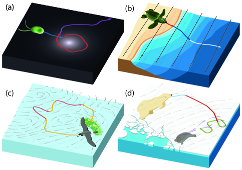
Figure 1: Examples menotaxis in animal movement: (a) Microalga positive phototaxis toward light (blue), perpendicular to maintain constant light intensity (red), then away from light (purple; Arrieta et al. 2017); (b) hatchling loggerhead sea turtles following visual cues toward brighter ocean (red), perpendicular orientation relative to waves to move away from shore (blue), and long-distance navigation guided by magnetic inclination (white; magnetotaxis) (Lohmann et al. 2008); (c) Desertas petrel transitory flights (yellow) approximately $50\degree$ relative to wind (grey field) and $80\degree$ during olfactory search (red) (Ventura et al. 2020); and (d) polar bear track at $15\degree$ relative to wind when stationary on sea ice (blue), approximately $90\degree$ relative to wind during olfactory search (red) to maximize probability of encountering odour plumes (purple), and movement apparently random relative to wind during area restricted search (green) (Togunov et al. 2017; 2018).

Identifying behaviours in movement data is a field of active development, and there is a need to develop more sophisticated movement models that consider the perceptual and cognitive capacities of animals (Auger-Méthé et al. 2016a; Bracis & Mueller 2017; Gaynor et al. 2019; Kays et al. 2015). Hidden Markov models (HMMs) are well-developed statistical models used to describe behavioural changes using movement data. HMMs and other movement models that integrate relationships between environmental data and movement characteristics (e.g., speed and orientation) have proven to be effective at elucidating interactions between movement and the environment (Kays et al. 2015; McClintock et al. 2020). Thus far, HMMs have only been used to model positive and negative taxis on turning angle. The detection of biased behaviours may also be confounded by mismatched spatial and temporal resolutions among data streams. Mismatched, multi-stream, multi-scale data are widespread in the field of spatial ecology and there is a need for statistical tools to integrate disparate data sources (Adam et al. 2019; Bestley et al. 2013; Fagan et al. 2013; Wilmers et al. 2015). In this paper, we first present an extension to BCRW HMMs that relaxes the direction of bias and allows modelling movement toward any angle relative to stimuli (i.e., menotaxis). Second, we propose incorporating a one-step transitionary state in HMMs when faced with low resolution environmental data to improve characterizing the direction of bias in BRWs. We investigate the accuracy of our model in two simulation studies and illustrate its application using polar bear telemetry data as a case study. Finally, we provide a detailed tutorial for these methods with reproducible R code in Appendix 1.

3 Methods

3.1 Model formulation

3.1.1 Introduction to modelling CRW, BRW, and basic BCRW

Animal movement observed using location data (i.e., latitude and longitude) is typically described using two data streams: step length $l_{t}\in(0,\infty)$ (distance between consecutive locations) and turning angle $\phi_{t}\in(-\pi,\pi]$ (change in bearing between consecutive steps), where $t\in 1,...,T$ represents the time of a step (Fig. 2; the notation used in this paper is described in Table 1). The probability of the step length $l_{t}$ from location at time $t$ to $t+1$ is often modelled with a Weibull or gamma distribution (Langrock et al. 2012; McClintock & Michelot 2018). We assume that $l_{t}$ is distributed as follows:

$$l_{t}\sim\mathrm{gamma}(\mu_{t}^{(l)},\sigma_{t}^{(l)}),\\$$ (1)

where $\mu_{t}^{(l)}\in(0,\infty)$ and $\sigma_{t}^{(l)}\in(0,\infty)$ are the mean and standard deviation of the step length (these parameters can also be derived from shape and scale parametrisation of the gamma distribution). Animal movement is often influenced by external factors that result in complex movement patterns (Auger-Méthé et al. 2016b). For example, some animals reduce speed when travelling through deep snow, increase speed when flying downwind, modulate orientation towards a foraging patch, or moving away from predators (Duchesne et al. 2015; McClintock & Michelot 2018; McClintock et al. 2012). The influence of these factors on movement can be represented by modelling the movement parameters as functions of external factors (e.g., McClintock & Michelot 2018). We can model behaviours where the mean speed of observed movement is associated with external factors using:

$$\mathrm{ln}(\mu_{t}^{(l)}) =\beta_{1}+\beta_{2}r_{t},$$ (2)

where $\beta_{1}\in(-\infty,\infty)$ is an intercept coefficient for step length mean and $\beta_{2}\in(-\infty,\infty)$ is a slope coefficient representing how the mean step length is affected by magnitude of external stimulus $r_{t}$ (e.g., wind speed, or speed of neighbouring individuals in a school of fish).

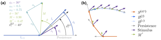
Figure 2: Illustration of the proposed menotactic BCRW for one step (a) and a sample three-state track (b). Panel (a) presents the notation used in this paper along with their values. Bold vectors represent values obtained from the data (animal track, blue vectors, and external stimulus, purple vector) and thin vectors represent values estimated by the model. $l_{t}$ and $l_{t-1}$ represent the step length, the light grey unit vector represents directional persistence from which turning angle $\phi_{t}$ is calculated. $\psi_{t}$ (purple arc) represents the angle of stimulus with magnitude $r_{t}$ relative to the bearing at $t-1$ (vector of persistence; light grey). The green arrow represents the vector of attraction with a magnitude of attraction $M$ and angle $\vartheta$ relative to stimulus, which are obtained from the estimated bias parallel, $\alpha_{1}$, and perpendicular, $\alpha_{2}$, to the stimulus (teal). $\mu_{t}^{(\phi)}$ (dark grey arc) represents the expected mean turning angle as a trade-off between persistence and bias toward $\vartheta$. $M^{\ast}$ represents the scaled magnitude of attraction. Panel (b) presents a sample track with a BCRW state with bias $\vartheta_{S^{(45\degree)}}=45\degree$ left of stimulus ($S^{(45\degree)}$; orange). A second BRW behaviour ($B$) with bias toward $\vartheta_{B}=-22\degree$ relative to stimulus is divide into a BRW state for the first step ($B^{(f)}$; blue) and a CRW state for consecutive steps ($B^{(c)}$; light blue). Green vector represents the scaled magnitude of attraction $M^{\ast}$ with direction $\vartheta$ relative to the stimulus. To represent environmental error, the true direction of the stimulus (not shown) rotates $-10\degree$ each step, while the estimated stimulus (purple) rotates $-5\degree$ each step.

Table 1: Description of acronyms and notation used in this paper and their interval, if applicable.

Acronym/variable	Interval	Description
CRW	-	Correlated random walk.
BRW	-	Biased random walk.
BCRW	-	Biased correlated random walk.
TBCRW	-	Biased correlated random walk incorporating     transitionary states.
$\pi$	$\pi$	The value 3.14159…
$T$	$\{1,2,...\}$	Total number of time steps.
$t$	$[1,T]$	A time step.
$X_{t}$	-	Set of observations at time $t$.
X	-	The set of all observations $(X_{1},...,X_{T})$.
$l$	$[0,\infty)$	Step length between consecutive locations.
$\phi$	$(-\pi,\pi]$	Turning angle (i.e., change in bearing) between     consecutive steps.
$r$	$[0,\infty)$	Magnitude of the stimulus.
$\psi$	$(-\pi,\pi]$	Direction of a stimulus relative to the bearing of the     previous time step.
$\mu^{(l)}$	$(0,\infty)$	Mean parameter of step length.
$\sigma^{(l)}$	$(0,\infty)$	Standard deviation parameter of step length.
$\beta_{1}$	$(-\infty,\infty)$	Intercept coefficient for mean step length.
$\beta_{2}$	$(-\infty,\infty)$	Slope coefficient for mean step length and $r$.
$\mu^{(\phi)}$	$(-\pi,\pi]$	Mean parameter of turning angle.
$\kappa^{(\phi)}$	$(0,\infty)$	Concentration parameter of turning angle.
$\alpha_{1}$	$(-\infty,\infty)$	Bias coefficient in the same direction as the stimulus.
$\alpha_{2}$	$(-\infty,\infty)$	Bias coefficient $90\degree$ left of the stimulus.
$\vartheta$	$(-\pi,\pi]$	The direction of bias relative to stimulus.
$M$	$[0,\infty)$	Magnitude of attraction.
$M^{\ast}$	$[0,1)$	Scaled magnitude of attraction.
HMM	-	Hidden Markov model.
$N$	$\{1,2,...\}$	Total number of behavioural states.
$S$	$[1,N]$	Behavioural state.
$\gamma_{i,j}$	$[0,1]$	Transition probability from state i to state j.
$\mathbf{\Gamma}$	-	$N\times N$ Transition probability matrix.
$B,B^{(f)},B^{(c)}$	-	A BRW state, a state for the first step in the BRW,     and a state for consecutive BRW steps, respectively.
$D,D^{(f)},D^{(c)}$	-	The drift state, a state for the first step in drift,     and a state for consecutive drift steps, respectively.
$O^{(L)},O^{(R)}$	-	Olfactory search state with anemotaxis left of wind     and anemotaxis right of wind, respectively.
$ARS$	-	Area restricted search state.

The probability of turning angle $\phi_{t}$ is often modelled with a wrapped Cauchy or von Mises distribution (McClintock et al. 2020). We assume that $\phi_{t}$ follows a von Mises distribution as follows:

$$\phi_{t}\sim\mathrm{vMises}(\mu_{t}^{(\phi)},\kappa_{t}^{(\phi)})$$ (3)

where $\mu^{(\phi)}_{t}\in(-\pi,\pi]$ is the mean turning angle parameter at time $t$ and $\kappa^{(\phi)}\in(0,\infty)$ is the concentration parameter around $\mu_{t}^{(\phi)}$ (Fig. 2a). In a basic CRW, $\mu_{t}^{(\phi)}$ is assumed to equal zero and only the concentration parameter $\kappa^{(\phi)}$ is modelled. In BRW and BCRW with simple positive or negative taxis (i.e., bias toward or away from a target), the mean turning angle $\mu_{t}^{(\phi_{t})}$ can be modelled as a function of the orientation relative to a stimulus $\psi_{t}$ (e.g., direction of den site; Fig. 2; McClintock & Michelot 2018); we assume $\phi_{t}$ follows a circular-circular von Mises regression model based on Rivest & Duchesne (2016):

$$\mu_{t}^{(\phi)}=\mathrm{atan2}(\alpha_{1}\sin\psi_{t},1+\alpha_{1}\cos\psi_{t})\\$$ (4)

where $\psi_{t}\in(-\pi,\pi]$ is the observed angle of stimulus at $t$ relative to the movement bearing at $t-1$ and $\alpha_{1}\in(-\infty,\infty)$ is the bias coefficient in the direction $\psi_{t}$ (Fig. 2a).

3.1.2 Extending the BCRW to allow for menotaxis

The BCRW described above can capture many behaviours exhibiting positive or negative taxis. However, many species exhibit menotactic movement where bias may be toward any angle relative to a stimulus (Fig. 1). To capture behaviours with a bias toward an unknown angle of attraction $\vartheta$ relative to $\psi_{t}$, we propose modelling the mean turning angle as a trade-off between directional persistance, bias parallel to the direction of the stimulus, and bias perpendicular to the stimulus (Figs. 2a and 3) following:

$$\mu_{t}^{(\phi)}=\mathrm{atan2}( \alpha_{1}\sin\psi_{t}+\alpha_{2}\cos\psi_{t},$$

$$1+\alpha_{1}\cos\psi_{t}-\alpha_{2}\sin\psi_{t}),$$ (5)

where $\alpha_{1}$ represents the attraction coefficient parallel to $\psi_{t}$ as in Eq. 4, and $\alpha_{2}\in(-\infty,\infty)$ represents the bias coefficient toward $90\degree$ anti-clockwise of $\psi_{t}$. In this framework, the centre angle of attraction relative to a stimulus is represented by $\vartheta=\mathrm{atan2}(\alpha_{2},\alpha_{1})$. Figs. 2 and 3 depict how the mean turning angle is controlled by the two bias coefficients $\alpha_{1}$ and $\alpha_{2}$ and the angle of stimuli $\psi_{t}$.

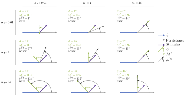
Figure 3: Illustration of various values of $\alpha_{1}$ and $\alpha_{2}$ and the corresponding direction of bias ($\vartheta$; green arc) relative to stimulus ($\psi_{t}=45\degree$; purple), scaled magnitude of attraction ($M^{\ast}$; green vector). The expected turning angle ($\mu_{t}^{(\phi)}$; dark grey) is calculated as a trade-off between directional persistence (light grey) from the proceeding step (blue) and bias toward vector of attraction. For clarity, the dashed line in the first panel represents direction of $\vartheta$.

Given the non-linear circular-circular link function, the slope of Eq. 3.1.2 varies with $\psi_{t}$ and results in artefacts that may not be ecologically meaningful (e.g., a negative slope or slopes approaching $\infty$; see Appendix A). We present an alternate formulation of $\mu_{t}^{(\phi)}$ with respect to $\psi_{t}$ with a constant slope in Appendix A, however this cannot currently be implemented in user-friendly R packages such as momentuHMM.

We can represent where along the spectrum of CRW and BRW a behaviour lies with the magnitude of attraction $M=\sqrt{\alpha_{1}^{2}+\alpha_{2}^{2}}\in[0,\infty)$. A value of $M=0$ represents a CRW, values around 1 represent BCRWs with equal weight for directional persistence and bias toward $\vartheta$, and values approaching infinity represent BRWs toward $\vartheta$. For a more intuitive metric, we can scale $M$ to the unit interval using:

$$M^{\ast}=\frac{M}{1+M}$$ (6)

where $M^{\ast}\in[0,1)$ represents the scaled magnitude of attraction. The CRW and BRW are limiting cases of Eq. 6, where $M^{\ast}\rightarrow 0$ and $M^{\ast}\rightarrow 1$, respectively, while a BCRW would have an intermediate value of $M^{\ast}$.

3.1.3 Integrating multiple states using hidden Markov models

Animal movement is behaviour-specific, and HMMs can be used to model telemetry data spanning multiple behaviours (Langrock et al. 2012; Patterson et al. 2008). Using HMMs, we can combine multiple behaviours with distinct types of biased and correlated movement patterns. HMMs are defined by two components: an unobserved state process (or hidden/latent process) and an observed state-dependent process. The state process assumes that animal behaviours are discrete latent states, $S_{t}\in\{1,...,N\}$, whose probabilities at any given time $t$ depend only on the state at the previous time step. That is, the state sequence $(S_{1},...,S_{T})$ follows a Markov chain governed by state transition probabilities $\gamma_{i,j}=\mathrm{Pr}(S_{t+1}=j|S_{t}=i)$ for $i,j\in\{1,...,N\}$, which are summarized by the $N\times N$ transition probability matrix, $\mathbf{\Gamma}=(\gamma_{i,j})$. Second, the state-dependent process $\textbf{X}=(X_{1},...,X_{T})$ (where $X_{t}=\{l_{t},\phi_{t}\}$) assumes that the probability of any given observation $X_{t}$, also known as the emission probability, depends only on the underlying latent state $S_{t}$ (Langrock et al. 2012; Patterson et al. 2008; Zucchini et al. 2016). That is, the step length and turning angle parameters and their respective coefficients (i.e., $\mu_{t}^{(l)},\sigma_{t}^{(l)},\mu_{t}^{(\phi)},\kappa_{t}^{(\phi)},\beta_{1},\beta_{2},\alpha_{1},\alpha_{2}$) are assumed to be state-specific (i.e., $\mu_{S,t}^{(l)},\sigma_{S,t}^{(l)},...$).

For some behaviours, we may expect animals to have two different, but related, angles to stimuli. For example, during cross-wind movement, we may expect the animal to move $90\degree$ to the left or right of the wind (i.e, ${\mu_{t}^{(\phi)}}=\psi_{t}\pm 90\degree$). Such behaviours will have a bimodal distribution for their turning angle ${\mu_{t}^{(\phi)}}$ relative to stimulus $\psi_{t}$, which would be difficult to model with a single distribution. However, we can model such behaviour with two states: biased left of stimulus ($S^{(L)}$ with bias toward $\psi_{t}+\vartheta_{S^{(L)}}$) and biased right of stimulus ($S^{(R)}$ with bias toward $\psi_{t}-\vartheta_{S^{(R)}}$). To reduce the number of estimated coefficients, these two states can share their parameters: $\kappa^{(\phi)}_{S^{(L,R)}}$, $\mu^{(l)}_{S^{(L,R)}}$, $\sigma^{(l)}_{S^{(L,R)}}$, and transition probabilities into and out of those states $\gamma_{i,j}$. If $\vartheta_{S^{(L)}}$ and $\vartheta_{S^{(R)}}$ are assumed to be symmetrical about $\psi_{t}$, $\alpha_{1,S}$ and $\alpha_{2,S}$ could be shared between symmetrical states by ensuring that $\alpha_{1,S^{(L)}}=\alpha_{1,S^{(R)}}$ and $\alpha_{2,S^{(L)}}=-\alpha_{2,S^{(R)}}$ in Eq. 3.1.2.

3.1.4 Accounting for mismatch in resolutions of data streams

The spatiotemporal resolution of data must be considered in research designs (Adam et al. 2019; Bestley et al. 2013; Fagan et al. 2013; McClintock et al. 2020). If there is a significant mismatch in the resolutions among data streams, BCRW models may favour the higher resolution data streams, potentially at the expense of biological accuracy. Although the preferred direction of a BRW is primarily determined by external factors rather than the direction of the preceding step, the movement often appears correlated because the direction of bias is also highly correlated (e.g., biased towards a distant target or toward temporally correlated stimulus; Fig. 2b; Benhamou 2006). If persistence explains more of the observed orientation than environmental data, BCRW models may incorrectly classify BRWs as CRWs (Benhamou 2006; Codling et al. 2008). This misclassification can occur if location resolution is very high or significantly higher than the environmental data, if environmental error is higher than the location data, or if the direction of stimulus remains relatively homogenous such that only the initial change in orientation exhibits taxis (Fig. 2b). Therefore, the first step in a BRW should be better explained by the environment than persistence even in the presence of error in environmental data (Fig. 2b).

To remedy the information loss associated with inadequate environmental data, we propose leveraging the information in the initial change in orientation by modelling the first step of a BRW state $B^{(f)}$ as a separate transition state from consecutive steps $B^{(c)}$. To ensure $B^{(f)}$ is modelled as a BRW, we must fix $\alpha_{1,B^{(f)}}$ or $\alpha_{2,B^{(f)}}$ to a large (positive or negative) value depending on the expected value of $\vartheta_{B^{(f)}}$. Second, to ensure that $B^{(f)}$ is fixed to just the first step in a BRW, we must ensure all states go through $B^{(f)}$ to get to $B^{(c)}$, that $B^{(f)}$ instantly transitions to $B^{(c)}$, and that $B^{(c)}$ cannot transition to $B^{(f)}$. These relationships can be enforced by ensuring the transition probability matrix $\mathbf{\Gamma}$ follows:

$$\mathbf{\Gamma}=\bordermatrix{&B^{(f)}&B^{(c)}&3&\ldots&N\cr B^{(f)}&0&1&0&\ldots&0\cr B^{(c)}&0&\gamma_{B^{(c)},B^{(c)}}&\gamma_{B^{(c)},3}&\ldots&\gamma_{B^{(c)},N}\cr 3&\gamma_{3,B^{(f)}}&0&\gamma_{3,3}&\ldots&\gamma_{3,N}\cr\vdots&\vdots&\vdots&\vdots&\ddots&\vdots\cr N&\gamma_{N,B^{(f)}}&0&\gamma_{N,3}&\ldots&\gamma_{N,N}\cr}.$$ (7)

To reduce the number of coefficients, the step length coefficients in Eq. 1 can be shared between $B^{(f)}$ and $B^{(c)}$. This method can be applied to any BRW state where the orientation of first step in the state is largely independent of the preceding step; including passive states driven by advection or strongly biased active states.

3.2 Simulation study

We conducted simulation studies to test two aspects of our proposed menotactic HMM. First, we validated the ability of our extended BCRW HMM to accurately recover states. Second, we investigated the effect of coarse environmental data on state detection and the ability of incorporating a one-step transitionary state to mediate the effects of environmental error. We used our polar bear case study as a base to develop the framework of our simulation studies.

3.2.1 Polar bear ecology background

We investigated three key behaviours: a passive BRW drift state, a BCRW olfactory search state, and a CRW area restricted search state. The prime polar bear foraging habitat is the offshore pack ice during the winter months (approximately January to May, depending on regional phenology; Pilfold et al. 2012; Stirling & McEwan 1975). The persistent motion of pack ice creates perpetual motion in the observed tracks, even when bears are stationary (e.g., still-hunting, prey handling, resting). One of the key drivers of sea ice motion is surface winds, whereby drift speed is approximately 2% of that of wind speed and approximately -20°relative to the wind direction (Tschudi et al. 2010). Passive drift can be modelled as a BRW, with a predicted $\vartheta\approx\pm 20\degree$ (Fig. 1d).

In the spring, polar bears’ primary prey, ringed seals (Pusa hispida) occupy subnivean lairs for protection from predators and the environment (Chambellant et al. 2012; Florko et al. 2020; Smith & Stirling 1975). Due to the large scale of the sea ice habitat and the cryptic nature of seals, polar bears rely heavily on olfaction to locate prey (Stirling & Latour 1978; Togunov et al. 2017; 2018). The theoretical optimal search strategy for olfactory predators when they do not sense any prey is to travel cross-wind (Baker et al. 2018; Kennedy & Marsh 1974; Nevitt et al. 2008), a pattern exhibited by polar bears (Togunov et al. 2017; 2018). Olfactory search can be modelled as a BCRW, with a predicted $\vartheta\approx\pm 90\degree$ (Fig. 1d). When in an area with suspected food availability, animals often exhibit decreased movement speed and increased sinuosity to increase foraging success (Potts et al. 2014), which has been documented in polar bears (Auger-Méthé et al. 2016a). Such area restricted search can be modelled as an unbiased CRW (Fig. 1d Auger-Méthé et al. 2015; Potts et al. 2014).

3.2.2 Track simulation

We simulated movement tracks using a four-state HMM with drift $D$, olfactory search left of wind $O^{(L)}$, olfactory search right of wind $O^{(R)}$, and area restricted search $ARS$. The $D$ and $O^{(L,R)}$ states were biased in relation to uniquely simulated wind fields. Wind fields were generated in four steps: simulating pressure fields, deriving longitudinal and latitudinal pressure gradients, re-scaling the pressure gradients to represent wind velocities, and finally applying a Coriolis rotation to obtain final wind vectors (see Appendix B for detail).

The $D$ state was defined as a passive BRW with mean step length determined by wind speed following Eq. 2, and turning angle following Eq. 6 with bias toward $\vartheta_{D}=-15\degree$, as estimated from the polar bear case study below. $O^{(L)}$ and $O^{(R)}$ were defined as BCRWs following Eq. 6 with biases toward $\vartheta_{O^{(L)}}=90\degree$ and $\vartheta_{O^{(R)}}=-90\degree$ relative to wind and a large mean step length. Last, $ARS$ was defined as a CRW with no bias relative to wind and low mean step length. All coefficients used in the simulation are presented in Table 2. All tracks were simulated using the momentuHMM package (see Appendix 1 for details; McClintock & Michelot 2018).

Table 2: Coefficients used to simulate the four-state BCRW HMM movement track (left side) and the corresponding bias parameters (right side). Non-applicable values are indicated by ‘-’.

State	$\beta_{1,S}$	$\beta_{2,S}$	$\sigma_{S}^{(l)}$	$\alpha_{1,S}$	$\alpha_{2,S}$	$\kappa_{S}^{(\phi)}$	$\vartheta_{S}(\degree)$	$M_{S}^{\ast}$
$D$	-2.2	0.1	-2.4	100	-26.8	5	-15	0.99
$O^{(L)}$	0.1	-	-0.5	0	5	2	90	0.83
$O^{(R)}$	0.1	-	-0.5	0	5	2	-90	0.83
$ARS$	-2.5	-	-2.8	0	-	0.5	-	0

In the first simulation study, movement relative to wind, $\psi_{t}$, was estimated from interpolated longitudinal and latitudinal pressure fields. In the second simulation study, the longitudinal and latitudinal wind fields were first spatially averaged to six resolutions (1, 2, 4, 8, 16, and 32 km) using the raster package (Hijmans & van Etten 2016) then interpolated. For both simulation studies, we evaluated model accuracy by first predicting states from fit HMMs using the Viterbi algorithm (Zucchini et al. 2016), merging analogous states (i.e., first drift $D^{(f)}$ and consecutive drift $D^{(c)}$; and $O^{(L)}$ and $O^{(R)}$), then calculating the proportion of correctly identified states (number of correctly identified steps / total number of steps). We also calculated recall (proportion of a simulated state correctly identified) for $D$ following $\sum$(correctly predicted $D$)/ $\sum$(simulated $D$).

3.2.3 Fitting HMMs to simulations

The first simulation validated the ability of our extended BCRW HMM to accurately recover states by comparing our model to a simpler CRW HMM. We fit 100 simulated tracks with two models: a three-state CRW HMM where mean drift speed was determined by wind but no states exhibit bias (e.g., Ventura et al. 2020) and a four-state BCRW HMM with wind-driven drift speed and bias in two states.

As the CRW HMM assumes no bias is present, the mean turning angle was fixed to zero and not estimated for any state ($\mu_{S}^{(\phi)}=0$). The BCRW HMM was formulated following the methods described in 3.2.2, with the $D$ and $O^{(L)}$ and $O^{(R)}$ states defined as biased relative to wind with both $\alpha_{1}$ and $\alpha_{2}$ being estimated. As we are primarily interested in differentiating the effect of incorporating menotaxis, the $D$ state step length was modelled as a function of wind speed as in Eq. 2 in both CRW and BCRW HMMs.

The second simulation study evaluated the effect of incorporating a transition state to alleviate information loss with lower environmental resolution. We down-scaled 100 simulations to six resolutions and fit two HMMs: the same four-state BCRW HMM used to simulate the tracks and a five-state HMM with drift divided into state for the first drift step $D^{(f)}$ and consecutive drift steps $D^{(c)}$ (hereafter, TBCRW HMM). Each simulated track was fit to the BCRW and TBCRW HMMs, which were compared by calculating the difference between their respective accuracies.

Drift was assumed to be a passive BRW relative to wind, which was ensured by fixing $\alpha_{1,D^{(f)}}$ to a large constant (in our case, $\alpha_{1,D^{(f)}}=100$) as described in 3.1.4. $D^{(c)}$ was modelled as a biased state with respect to wind, however given the low resolution of wind data, no assumption was made on the direction of the bias relative to wind. Olfactory search was modelled as two states $O^{(L)}$ and $O^{(R)}$ that were biased with respect to wind, and we assumed these to be symmetrical about $0\degree$. Finally, we assumed $ARS$ to be a CRW independent of wind. These were modelled by modifying Eq. 3.1.2 to:

$$\mu_{S,t}^{(\phi)}=\begin{cases}\begin{aligned} &0\\ &\mathrm{atan2}(100\sin\psi_{t}+\alpha_{2,S}\cos\psi_{t},\\ &\quad\quad\quad 1+100\cos\psi_{t}-\alpha_{S,2}\sin\psi_{t})\\ &\mathrm{atan2}(\alpha_{1,S}\sin\psi_{t}-\alpha_{2,S}\cos\psi_{t},\\ &\quad\quad\quad 1+\alpha_{1,S}\cos\psi_{t}+\alpha_{2,S}\sin\psi_{t})\\ &\mathrm{atan2}(\alpha_{1,S}\sin\psi_{t}+\alpha_{2,S}\cos\psi_{t},\\ &\quad\quad\quad 1+\alpha_{1,S}\cos\psi_{t}-\alpha_{2,S}\sin\psi_{t})\\ \end{aligned}\end{cases}\quad\begin{aligned} &\mathrm{if}\>S=ARS\\ &\mathrm{if}\>S=D^{(f)}\\ \\ &\mathrm{if}\>S=O^{(R)}\\ \\ &\mathrm{Otherwise.}\\ \\ \end{aligned}$$ (8)

To reduce the number of estimated coefficients, the coefficients for step length ($\beta^{(l)}_{1,S}$, $\beta^{(l)}_{2,S}$, and $\sigma^{(l)}_{S}$) were shared between $D^{(c)}$ and $D^{(f)}$ and between $O^{(L)}$ and $O^{(R)}$. For $O^{(L)}$ and $O^{(R)}$, $\kappa^{(\phi)}$, $\alpha_{1,S}$, and $\alpha_{2,S}$ were also shared along with the state transition probabilities $\gamma_{i,j}$. To ensure $D^{(f)}$ lasts one step, we fixed the transition probabilities following equation 7. The transition probability matrix contained nine coefficients to be estimated following:

$$\mathbf{\Gamma}=\bordermatrix{&D^{(f)}&D^{(c)}&O^{(L)}&O^{(R)}&ARS\cr D^{(f)}&0&1&0&0&0\cr D^{(c)}&0&\gamma_{2,2}&\gamma_{2,3}&\gamma_{2,3}&\gamma_{2,5}\cr O^{(L)}&\gamma_{3,1}&0&\gamma_{3,3}&\gamma_{3,4}&\gamma_{3,5}\cr O^{(R)}&\gamma_{3,1}&0&\gamma_{3,4}&\gamma_{3,3}&\gamma_{3,5}\cr ARS&\gamma_{5,1}&0&\gamma_{5,3}&\gamma_{5,3}&\gamma_{5,5}\cr}$$ (9)

3.3 Case study - Polar bear olfactory search and drift

We illustrate the application of our HMM using global positioning system (GPS) tracking data from one adult female polar bear collared as part of long-term research on polar bear ecology (Lunn et al. 2016). The performed animal handling and tagging procedures were approved by the University of Alberta Animal Care and Use Committee for Biosciences and by the Environment Canada Prairie and Northern Region Animal Care Committee (Stirling et al. 1989). We limited the analysis to one month during the peak foraging period between Apr 5, 2011 and May 5, 2011. The collar was programmed to obtain GPS locations at a 30 min frequency. To obtain the continuous environmental data necessary for HMMs, missing locations (n = 8; 0.56%) were imputed by fitting a continuous-time correlated random walk model using the crawl package in R (Johnson & London 2018; Johnson et al. 2008; R Core Team 2020). GPS locations were annotated with wind data using the ERA5 meteorological reanalysis project, which provides hourly global analysis fields at a 31 km resolution (Hersbach et al. 2020). Wind estimates along the track were interpolated in space and time as described in Togunov et al. (2017; 2018). We modelled the polar bear track as a five-state TBCRW HMM as in the second simulation. All statistical analyses were done in R version 4.0.2 (R Core Team 2020). Reproducible code is presented in Appendix 1.

4 Results

4.1 Simulation

The first simulation served to validate that the proposed BCRW HMM can accurately recover states. As expected, the accuracy (mean and [2.5%, 97.5%] quantiles) of the BCRW HMM (0.96 [0.96, 0.96]) was higher than that of the unbiased CRW HMM (0.77 [0.77, 0.78]). In both models, olfactory search was the most accurately identified state (Table C1). The BCRW HMM had higher precision in estimating all states compared to the CRW HMM. The CRW HMM had the lowest precision rate when predicting $D$, where it more frequently confused it for $ARS$ (Table C1).

When there was no environmental error, the basic BCRW HMM outperformed the TBCRW HMM (Fig. 4). As the environmental resolution declined, the accuracy of both models also declined, however, the TBCRW HMM outperformed the BCRW HMM at resolutions coarser than 4 km (Fig. 4). At finer resolutions, recall (mean and [25%, 75%] quantiles) of $D$ in the BCRW HMM was higher than in TBCRW HMM (e.g., $\mathrm{recall}_{BCRW,1\mathrm{k}m}=0.88[0.84,0.91]$ vs $\mathrm{recall}_{TBCRW,1\mathrm{k}m}=0.74[0.69,0.77]$). At resolutions coarser than 8 km, recall of $D$ in the BCRW HMM was lower than in the TBCRW HMM (e.g., $\mathrm{recall}_{BCRW,32\mathrm{k}m}=0.40[0.31,0.46]$ vs $\mathrm{recall}_{TBCRW,32\mathrm{k}m}=0.61[0.54,0.67]$).

In both the BCRW HMM and TBCRW HMM, the mean estimates of $\vartheta_{D}$, $\vartheta_{D^{(f)}}$, and $\vartheta_{D^{(c)}}$ across the 100 simulated tracks were close to the simulated $-15\degree$, however, there was a marked difference in the spread of estimates across the simulations (Fig. 5a). At resolutions 4 km or finer, the BCRW HMM provided reasonable estimates of $\vartheta_{D}$ and $M^{\ast}$ ($\geq 79\%$ of $\hat{\vartheta}_{D}\in\vartheta_{D}\pm 5\degree$; Fig. 5). At resolutions coarser than 4 km, the spread of estimated values increased with $\leq 30\%$ of $\hat{\vartheta}_{D}\in\vartheta_{D}\pm 5\degree$ (Fig. 5a). According to the BCRW HMM, at a 16 km resolution, $D$ would be characterized as a BCRW ($M^{\ast}_{D}\approx 0.5$) and a BRW at 32 km ($M^{\ast}_{D,t}\approx 0$; Fig. 5b). These patterns were exaggerated for the $D^{(c)}$ state in the TBCRW HMM, with the estimates of $\vartheta_{D^{(c)}}$ widening at 4 km resolutions and coarser and the rate of change $M^{\ast}_{D^{(c)}}$ suggested $D^{(c)}$ was a CRW (Fig. 5). In contrast, the transitionary $D^{(f)}$ state in the TBCRW HMM was estimated more accurately than either $D^{(c)}$ or $D$, with more estimates of $\vartheta_{D^{(f)}}$ closer to the simulated $-15\degree$ at all resolutions (Fig. 5a).

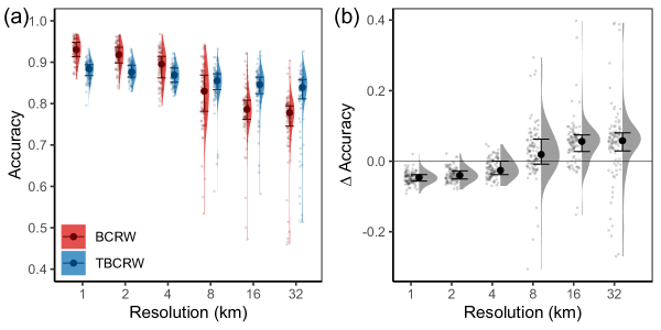
Figure 4: State prediction accuracy (a) and difference in accuracy (b) between the biased correlated random walk (BCRW) and transitionary-BCRW (TBCRW) HMMs ($\Delta$ accuracy = $\mathrm{accuracy_{TBCRW}-accuracy_{BCRW}}$). The accuracies of the 100 individual simulated tracks are represented by the transparent points, shaded areas represent the density across the 100 tracks, and opaque points represent the medians. Error bars span the 25% and 75% quantiles of the accuracies.

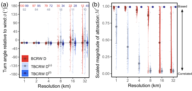
Figure 5: Estimated direction of bias relative to wind $\vartheta$ (a) and scaled magnitude of attraction $M^{\ast}$ (b) for the drift state ($D$) in the biased correlated random walk (BCRW) HMM (red), and first drift ($D^{(f)}$; blue) and consecutive drift ($D^{(c)}$; teal) states of the transitionary-BCRW (TBCRW) HMM. Values at the top of (a) represent what percent of the simulation runs estimated $\vartheta$ within $-15\pm 5\degree$ for each model. Points represent the raw estimates from the 100 simulated tracks, shaded areas represent the density across the 100 tracks, and opaque points represent the medians. Error bars span the 25% and 75% quantiles of the estimates.

4.2 Case Study: Polar bear olfactory search and drift

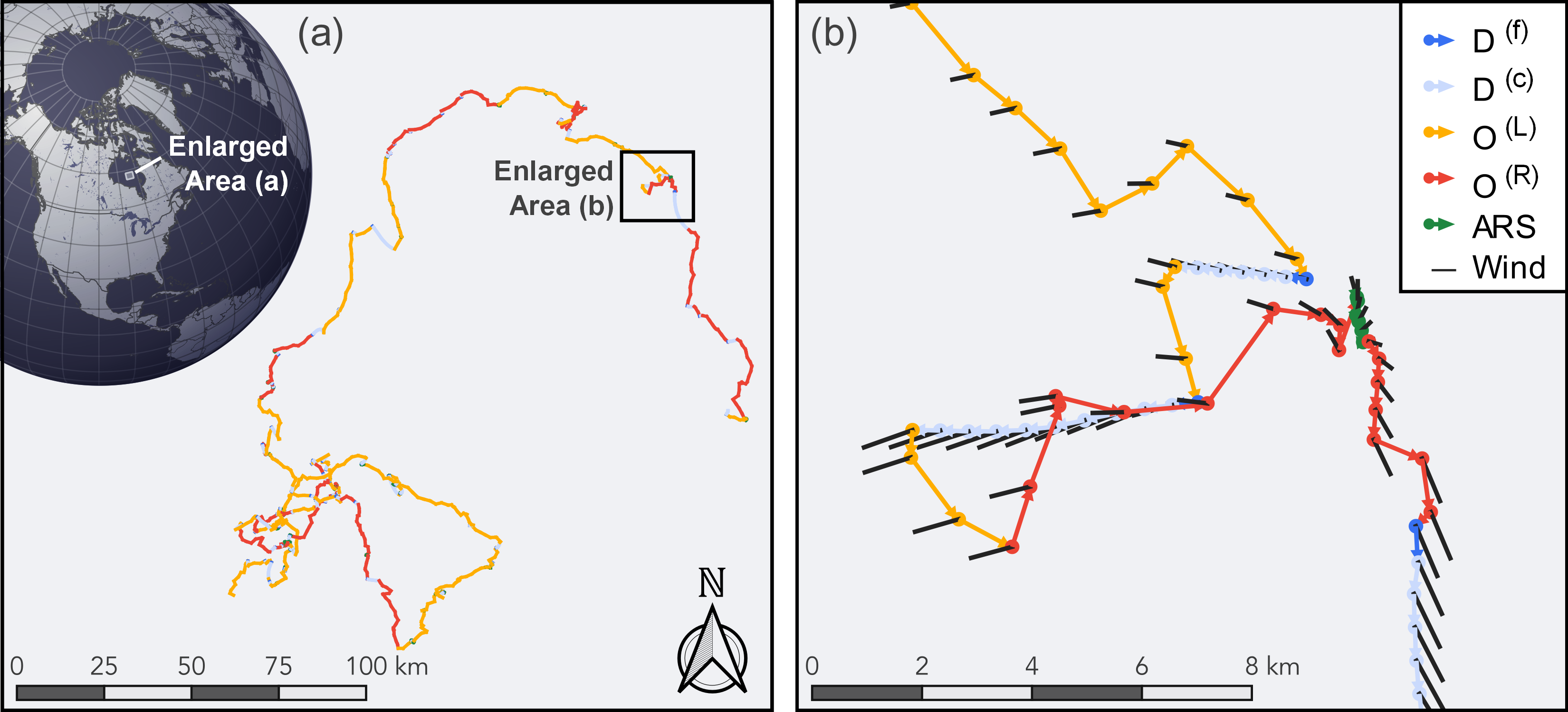
Figure 6: GPS track of a polar bear in spring 2011. Colours represent the predicted states of a five-state HMM determined using the Viterbi algorithm. Black lines represent direction and magnitude of wind.

The fitted HMM showed distinct movement characteristics among the five modelled states. Based on the stationary state distribution, the bear spent about 35% of its time between $D^{(c)}$ and $D^{(f)}$, 47% between $O^{(L)}$ and $O^{(R)}$, and 17% in $ARS$. The only notably differences in transition probabilities were that $D^{(c)}$ was more likely to be followed by $O^{(L,R)}$ than $ARS$ and that the transition between $O^{(L)}$ and $O^{(R)}$ was significantly less likely than the probability of remaining within the same olfactory search state (Table 3).

Table 3: Estimated transition probability matrix, $\mathbf{\Gamma}$, for polar bear HMM. Values represent transition probabilities, $\gamma_{i,j}\pm\mathrm{SE}$ (estimated using momentuHMM; McClintock & Michelot 2018), from state $i$ to $j$.

$$\mathbf{\Gamma}=\bordermatrix{&D^{(f)}&D^{(c)}&O^{(L)}&O^{(R)}&ARS\cr D^{(f)}&0&1&0&0&0\cr D^{(c)}&0&0.83\pm 0.02&0.07\pm 0.01&0.07\pm 0.01&0.02\pm 0.01\cr O^{(L)}&0.08\pm 0.01&0&0.83\pm 0.02&0.02\pm 0.01&0.07\pm 0.01\cr O^{(R)}&0.08\pm 0.01&0&0.02\pm 0.01&0.83\pm 0.02&0.07\pm 0.01\cr ARS&0.07\pm 0.02&0&0.08\pm 0.01&0.08\pm 0.01&0.77\pm 0.03\cr}$$

First drift, $D^{(f)}$, was characterized as a passive BRW with mean direction and speed determined by wind. As described in 3.2.3, the downwind bias coefficient was fixed to $\alpha_{1,D^{(f)}}=100$ to ensure it was a BRW and crosswind bias coefficient was estimated at $\alpha_{2,D^{(f)}}=-27.65$, corresponding to an overall bias toward $\vartheta_{D^{(f)}}=-15\degree$ relative to wind (Figs. 7b and 8a; Table 4). Turning angle concentration was moderate ($\kappa^{(\phi)}_{D^{(f)}}=1.61$) and scaled magnitude of attraction was very high ($M^{\ast}_{T}=0.99$), best characterizing $D^{(f)}$ as a BRW (Fig. 8a; Table 4).

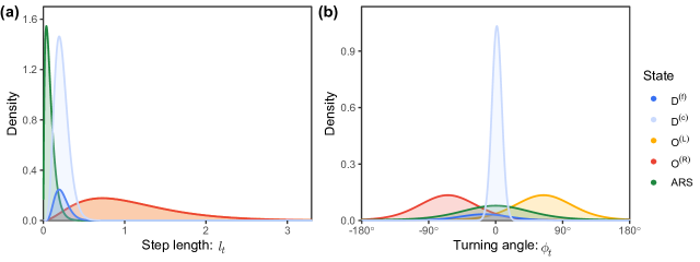
Figure 7: Probability density plots based on a fitted five-state HMM for (a) step length $l_{t}$ (km $30\mathrm{min}^{-1}$) assuming wind speed $r_{t}=6\mathrm{m\,s}^{-1}$ and (b) turning angle $\phi_{t}$ (in radians) assuming relative angle $\psi_{t}=0$. The height of each density distribution is scaled by the stationary state distribution of each respective state.

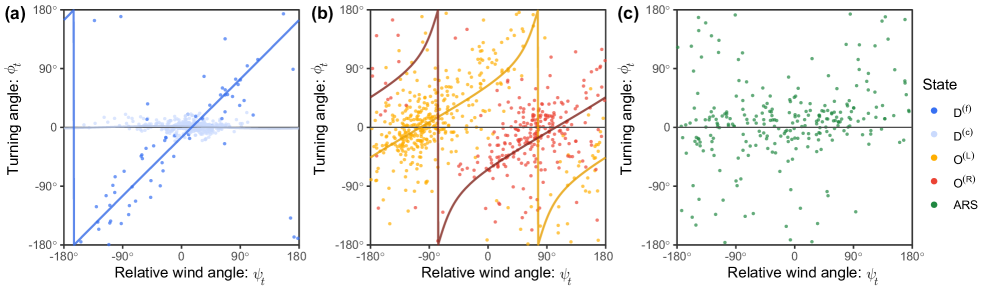
Figure 8: Turning angle $\phi_{t}$ (in radians) versus angle of wind relative to previous step $\psi_{t}$ (in radians). Lines represent the expected turning angle based on the estimated values of $\alpha_{1,S}$ and $\alpha_{2,S}$ given $\psi_{t}$.

Table 4: Estimated parameters and coefficients for five-state polar bear HMM.

Data stream	Parameter	Coefficient	States	Estimate (SE)
	$\mu^{(l)}$	$\beta_{1}$	$D^{(f)}$, $D^{(c)}$	-2.118 (0.042)
Step length		$\beta_{2}$	$D^{(f)}$, $D^{(c)}$	0.107 (0.004)
		$\beta_{1}$	$O^{(L)}$, $O^{(R)}$	0.087 (0.027)
		$\beta_{1}$	$ARS$	-2.501 (0.106)
	$\sigma^{(l)}$		$D^{(f)}$, $D^{(c)}$	-2.445 (0.037)
			$O^{(L)}$, $O^{(R)}$	-0.462 (0.044)
			$ARS$	-2.804 (0.153)
	$\mu^{(\phi)}$	$\alpha_{1}$	$D^{(f)}$	100 (0)
		$\alpha_{2}$	$D^{(f)}$	-27.645 (8.409)
		$\alpha_{1}$	$D^{(c)}$	-0.020 (0.015)
Turning angle		$\alpha_{2}$	$D^{(c)}$	0.027 (0.008)
		$\alpha_{1}$	$O^{(L)}$, $O^{(R)}$	-0.332 (0.062)
		$\alpha_{2}$	$O^{(L)}$, $O^{(R)}$	1.385 (0.125)
		$\mu^{(\phi)}$	$ARS$	0 (0)
	$\kappa^{(\phi)}$		$D^{(f)}$	1.131 (0.158)
			$D^{(c)}$	4.325 (0.112)
			$O^{(L)}$, $O^{(R)}$	0.843 (0.068)
			$ARS$	0.476 (0.138)

The mean observed direction of drift relative to wind was $13\degree$ (estimated from a von Mises distribution fit to the direction of wind for steps classified as $D^{(f)}$ or $D^{(c)}$). However, turning angle during $D^{(c)}$ showed almost no bias relative to wind ($\alpha_{1,D^{(c)}}=-0.02$ and $\alpha_{2,D^{(c)}}=0.03$; $M^{\ast}_{D^{(c)}}=0.03$) and turning angle concentration was very high ($\kappa^{(\phi)}_{D^{(c)}}=75.60$), thus best characterizing $D^{(c)}$ as a CRW with high persistence (Figs. 7b and 8a; Table 4). These results mirror those observed in the second simulation, which characterized $D^{(f)}$ as a BRW and $D^{(c)}$ as a CRW (Fig. 5). The step length of $D^{(f)}$ and $D^{(c)}$ were characterized by a small step length that was explained by an exponential relationship to wind speed (Fig. 9). At the median wind speed of 21.0 km h^-1, the mean step length of $D^{(f,c)}$ was $0.22\pm 0.09$ km 30m^-1 ($\mu^{(l)}_{D^{(f,c)}}\pm\sigma^{(l)}_{D^{(f,c)}}$), or $\approx 2\%$ of wind speed (Fig. 7a; Table 4).

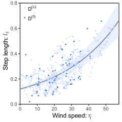
Figure 9: Curve representing the estimated mean step length parameter $\mu^{(l)}_{t}$ (in km 30m^-1) as a function of wind speed $r_{t}$ (in km h^-1). Shaded area represents 95% confidence interval. Points represent observed step lengths for first drift ($D^{(f)}$) and consecutive drift ($D^{(c)}$) states.

Olfactory search was characterized as a fast BCRW relative to wind. The estimated mean step length was $1.09\pm 0.63$ km ($\mu^{(l)}_{O^{(L)},O^{(R)}}\pm\sigma^{(l)}_{O^{(L)},O^{(R)}}$; Fig. 7a; Table 4). Bias downwind during olfactory search was $\alpha_{1,O^{(L)},O^{(R)}}=-0.332$ and bias crosswind was $\alpha_{2,O^{(L)},O^{(R)}}=\pm 1.385$, corresponding to an overall bias toward $\vartheta_{O^{(L)},O^{(R)}}=\pm 103\degree$ relative to wind (Figs. 7b and 8b; Table 4). The turning angle concentration was moderate ($\kappa^{(\phi)}_{O^{(L)},O^{(R)}}=2.324$) as was the scaled magnitude of attraction ($M^{\ast}_{O^{(L)},O^{(R)}}=0.588$), best characterizing olfactory search as a BCRW (Fig. 8b; Table 4).

ARS was characterized as a slow CRW with no bias relative to wind. The estimated mean step length was $0.08\pm 0.06$ km ($\mu^{(l)}_{ARS}\pm\sigma^{(l)}_{ARS}$; Fig. 7a; Table 4). Mean turning angle was fixed to zero and the turning angle concentration was the lowest among the states ($\kappa^{(\phi)}_{ARS}=1.61$), best characterizing ARS as a CRW with low persistence (Figs. 7b and 8c; Table 4).

5 Discussion

Behaviours with biased movement are common among animals for obtaining resources and avoid costs (Bailey et al. 2018; Michelot et al. 2017; Ylitalo et al. 2020). Here, we described two extensions to HMMs to identify and characterize menotaxic behaviours and BRWs. By modelling turning angle bias with a component parallel to and a component perpendicular to stimuli, menotexic behaviours with bias toward any angle can be modelled. Second, we outline the use of a one-step ‘transitionary’ state for taxic BRWs, which can improve the accuracy of state detection and estimation of the direction of bias when the resolution of the environmental data is coarse relative to the animal track. We illustrated the application of these methods for detecting olfactory search and passive drift from both simulated data and polar bear tracking data using the readily accessible and well documented momentuHMM package in R (McClintock & Michelot 2018). To further aid in the implementation of these methods, we have provided a tutorial with reproducible R code in Appendix 1.

Given the ubiquity of taxes exhibited among animals, other studies have integrated bias into their movement models. However, these have exclusively been simple attractive or repulsive bias (i.e., positive and negative taxis; e.g., Benhamou 2014; McClintock & Michelot 2018; Michelot et al. 2017). Further, although there has been much investigation into mechanisms and consequences of behaviours with nonparallel bias relative to the direction of stimuli, such menotaxis has yet to be mechanistically integrated in a movement model. Typically, menotaxis has been studied independently of the movement process or using post hoc analysis and is identified either using visual assessment or basic descriptive statistics (e.g., Mestre et al. 2014; Paiva et al. 2010; Togunov et al. 2017; 2018; Ventura et al. 2020). Such methods are appropriate for some analyses, however, they may prohibit investigating more nuanced relationships between animals, their behaviour, and the environment. The direction of taxis may be unknown, incorrectly assumed a priori, or may be affected by other factors (e.g., environmental covariates, internal state). Not accounting for these interactions may lead to incorrectly classifying movement or incorrectly estimating the direction or strength of bias. For instance, conventional methods for analysis of tracking data in mobile environments account for involuntary motion by simply subtracting the component of drift from the movement track (e.g., Blanchet et al. 2020; Gaspar et al. 2006; Klappstein et al. 2020; Safi et al. 2013). However, this type of correction does not account for the error often in the environmental data (Dohan & Maximenko 2010; Togunov et al. 2020; Yonehara et al. 2016). Our methods overcome some of these limitations by building on the robust framework of HMMs, which are relatively flexible to uncertainty in both the track and environmental data by distinguishing between latent state and state-dependent processes (McClintock et al. 2012; Zucchini et al. 2016).

Our first simulation study validated the ability of our proposed BCRW HMM (i.e., integrating anemotaxis into predicting the turning angle) to accurately identify states. Compared to an unbiased HMM, our method more reliably identified all three behavioural states, with a marked increase in accuracy (60 percentage points) for the drift state compared to more traditional HMM models. In cases where the speed of movement (i.e., step lengths) among different behaviours become more similar, a conventional HMM using only step length and turning angle may be completely unable to differentiate states, while our model may still be able to differentiate taxes.

When modelling measured data, the estimated parameters reflect both the underlying process of interest (e.g., a connection between movement, wind, and drift) as well as any underlying error in the data (Bestley et al. 2013). For instance, a low coefficient for a covariate may correctly reflect a weak ecological relationship or be an incorrect artefact of data with high error (Bestley et al. 2013). Our second simulation study demonstrated that at coarser resolutions of environmental data, a simpler BCRW HMM was prone to incorrectly characterizing BRWs as CRWs. We showed that the use of a one-step transitionary state can help recover some of the information lost for taxic BRWs in the presence of environmental error. The use of a transitionary state yielded two advantages: reduced misclassification of BRWs and improved estimation of the direction of bias. Although the use of a transitionary drift state caused consecutive drift steps to be misclassified as a CRW, the transitionary state was able to recover information on bias that would otherwise be lost entirely using conventional models. Employing a transitionary state for BRWs has one important caveat: because the transitionary state lasts for precisely one step, the model requires there to be a sufficient number of state transitions to the BRW for sufficient power to accurately estimate bias coefficients. To obtain a sufficient number of BRW transitions may require longer tracking or sharing coefficients among different animals. The utility of employing a transitionary state method depends on the system, but generally, it may be advantageous if the temporal resolution of the environmental data is coarser than the tracking data, if the angular error in the environmental data tends to be greater than the turning angle, or if high homogeneity in the environmental data carries error across multiple steps. In our case, the use of a transitionary state was beneficial as soon as the track data resolution was equal to or higher than the temporal resolution of the wind data (data not shown).

Different behaviours have unique fitness consequences and unique relationships with the environment, thus identifying the underlying behavioural context is critical to effectively interpret observed data (Roever et al. 2014; Wilson et al. 2012). This study was the first to identify stationary behaviour in polar bear tracking data, which made up a notable 35% of the track duration. The drifting state encapsulates several distinct behaviours including rest, sheltering during adverse conditions, still hunting by a seal breathing hole, or prey handling (Stirling 1974; Stirling et al. 2016). To distinguish between this mixture of behaviours we may investigate the effect of time or environmental conditions on the transition probabilities between states (i.e., relaxing the model assumption of homogenous state transition probability matrix). In some cases, the strength or direction of bias may depend on other factors. For example, bias to the centre of an animal’s home range may depend on its distance from that centre (McClintock et al. 2012), or the strength of bias relative to wind during passive advection being proportional to wind speed (e.g., Yu et al. 2020). Such interactions with the bias can be accomplished by modelling bias coefficients, $\alpha_{1}$ and $\alpha_{2}$, as functions of covariates (e.g., distance to target, or magnitude of stimuli). Another important extension is to model multiple biases simultaneously, as animal movement is often driven by several competing goals (e.g., navigation in flocking birds; Nagy et al. 2010). These extensions can all be readily accommodated using momentuHMM (McClintock & Michelot 2018). In cases where simultaneous biases interact in complex ways, more advanced extensions may be required (Mouritsen 2018). In mobile environments, such as birds in flight, the movement of the animal itself contains information on the flow since it is influenced by the currents and advection may affect the appearance of movement in all behaviours (Goto et al. 2017; Wilmers et al. 2015; Yonehara et al. 2016). If the magnitude of advection is comparable to the speed of voluntary movement, explicitly accounting for advection in all behaviours becomes increasingly important (Auger-Méthé et al. 2016b; Gaspar et al. 2006; Yonehara et al. 2016). Our model can serve as a starting point for modelling menotactic BCRWs without making assumptions on the strength or direction of bias or assuming error-free movement and environmental data. The methods we present in this paper are simple extensions to conventional movement models. They can be readily applied to animal tracking data to characterise menotactic behaviours and open new avenues to investigate more nuanced and mechanistic relationships between animals and their environment.

6 Acknowledgments

Financial and logistical support of this study was provided by the Canadian Association of Zoos and Aquariums, the Canadian Research Chairs Program, the Churchill Northern Studies Centre, Canadian Wildlife Federation, Care for the Wild International, Earth Rangers Foundation, Environment and Climate Change Canada, Hauser Bears, the Isdell Family Foundation, Kansas City Zoo, Manitoba Sustainable Development, Natural Sciences and Engineering Research Council of Canada, Parks Canada Agency, Pittsburgh Zoo Conservation Fund, Polar Bears International, Quark Expeditions, Schad Foundation, Sigmund Soudack and Associates Inc., Wildlife Media Inc., and World Wildlife Fund Canada. We thank B.T. McClintock for assistance with momentuHMM and E. Sidrow for reviewing the manuscript.

7 Authors’ contributions

RRT and MAM conceived the ideas and designed methodology; NJL and AED conducted fieldwork; RRT conducted the analyses and prepared the manuscript. All authors contributed critically to the drafts and gave final approval for publication.

8 Data Availability

The location data of the polar bear case study is available on UAL Dataverse (Derocher 2021). Code to reproduce the simulations and the case study is available on Zenodo (Togunov et al. 2021). Wind data were obtained from the ERA5 meteorological reanalysis project (Hersbach et al. 2020).

Appendix A Appendix: Turning Angle Link Function

In this paper, we modelled mean turning angle ${\mu_{S,t}^{(\phi)}}$ relative to external stimuli $\psi_{t}$ using the circular-circular link function of Rivest & Duchesne (2016). By modelling movement as a bias in the same direction as a stimulus $\alpha_{1}$ and a bias perpendicular to a stimulus $\alpha_{2}$, we can predict movement with a bias toward any angle relative to the stimulus Fig. A.1. However, the circular-circular (i.e., non-linear) link function produces artefacts that may not have ecological significance. First, we define the rate of change of ${\mu_{S,t}^{(\phi)}}$ with respect to $\psi_{t}$ (i.e., the turning angle rate of change) as the first-order derivative of Eq. 3.1.2

$${\mu_{S,t}^{(\phi)}}^{\prime}=\frac{\alpha_{1,S}^{2}+\alpha_{1,S}\cos(\psi_{t})+\alpha_{2,S}^{2}-\alpha_{2,S}\sin(\psi_{t})}{\alpha_{1,S}^{2}+2\alpha_{1,S}\cos(\psi_{t})+\alpha_{2,S}^{2}-2\alpha_{2,S}\sin(\psi_{t})+1}.$$ (10)

We might expect ${\mu_{S,t}^{(\phi)}}^{\prime}$ to be monotonically positive. For instance, as the direction of external stimuli rotate anti-clockwise, so should the predicted turning angle. The circular-circular distribution can produce negative values of ${\mu_{S,t}^{(\phi)}}^{\prime}$ occur when the the movement of a behaviour is closer to a CRW (i.e., magnitude of bias $\sqrt{\alpha_{1,S}^{2}+\alpha_{2,S}^{2}}<1$) and the movement is opposite to the direction of bias (i.e., $\psi_{t}\rightarrow-\vartheta+180\degree$; red and yellow curves in Fig. A.2 a). Second, values of ${\mu_{S,t}^{(\phi)}}^{\prime}\rightarrow\infty$ as $\sqrt{\alpha_{1,S}^{2}+\alpha_{2,S}^{2}}\rightarrow 1^{+}$; this occurs over a narrow interval of values of $\alpha_{1,S}$ and $\alpha_{2,S}$ and when movement is opposite the direction of bias (i.e., $\psi_{t}\rightarrow\vartheta+180\degree$; teal curve in Fig. A.2 a).

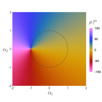
Figure A.1: The expected turning angle $\mu^{(\phi)}_{t}$ in degrees given values of $\alpha_{1}$ and $\alpha_{2}$, assuming movement is in the same direction as stimulus (i.e., $\psi_{t}=0\degree$). As $\psi_{t}$ increases, this plot would effectively rotate clockwise about $(\alpha_{1}=0,\alpha_{2}=0)$ by the value of $\psi_{t}$. When $\sqrt{(\alpha_{1}^{2}+\alpha_{2}^{2})}\geq 1$ (on or outside the circle), increasing increasing $\psi_{t}$ would always result in increasing turning angle. However, when $\sqrt{(\alpha_{1}^{2}+\alpha_{2}^{2})}<1$ (inside the circle) and as $|\psi_{t}|\rightarrow 180\degree$, increasing $\psi_{t}$ can result in decreasing turning angle.

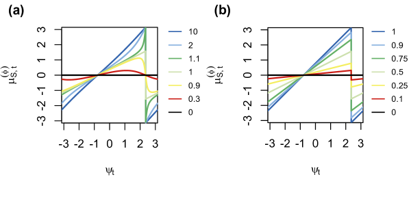
Figure A.2: Predicted turning angle ${\mu_{S,t}^{(\phi)}}$ relative to direction of stimulus $\psi_{t}$ assuming bias is toward $\vartheta=45\degree$. Panel ‘a’ represents the predicted turning angle using the circular-circular von Mises distribution of Rivest & Duchesne (2016). The $\alpha_{1,S}$ and $\alpha_{2,S}$ are constraint such that magnitude of attraction $M_{S}=\sqrt{\alpha_{1,S}^{2}+\alpha_{2,S}^{2}}$ is between 0 (black) and 10 (dark blue) as shown. Panel ‘b’ represents the predicted turning angle using our proposed circular-linear von Mises distribution defined in Eq. 11 with a attraction coefficient $\lambda_{S}$ between 0 (black) and 1 (dark blue) as shown. Both axes are in radians.

An alternative way to formulate biased behaviours is to model $\mu_{S,t}^{(\phi)}$ explicitly relative to a the direction of bias $\vartheta_{S}$ and the strength of bias. Specifically, assuming a von Mises distribution for turning angle, the predicted mean turning angle can be modelled by

$$\mu_{S,t}^{(\phi)}=\arctan\Big{(}\tan\frac{\psi_{t}+\vartheta_{S}}{2}\Big{)}2\lambda_{S},$$ (11)

where $\lambda_{S}\in[0,1]$ represents the state-specific bias coefficient trade-off between directional persistence and bias toward the expected state-specific orientation relative to stimulus $\vartheta_{S}\in(-\pi,\pi]$, and $\psi_{t}$ is the observed angle of stimulus relative to the movement bearing at time $t-1$ (Fig. 3). The tan and arctan arguments ensure that the predicted values of $\mu_{S,t}^{\phi}$ fall within $(-\pi,\pi]$ and that the functions are linear, and $\lambda_{S}$ is effectively the slope coefficient determining the strength of bias. Specifically, $\lambda_{S}=0$ represents a CRW (black in Fig. A.2 b), $\lambda_{S}=1$ represents a BRW toward $\vartheta_{S}$ (purple in Fig. A.2 b), and $\lambda_{S}=0.5$ represents a BCRW with equal weight to directional persistence and bias toward $\vartheta_{S}$ (green in Fig. A.2 b). This formulation directly models the parameters of interest and does not exhibit nonlinear artefacts as in the circular-circular distribution (Fig. A.2).

We developed our BCRW HMM using the momentuHMM package to be easily approachable and applicable. However, it is not currently possible to implement the circular-linear formulation described in Eq. 11. The only way to estimate both strength of movement bias and direction of bias in momentuHMM is using the circular-circular link function. Implementing the model using a circular-linear formulation would require writing a custom HMM, which may not be accessible to most practitioners. For most use-cases, the circular-circular distribution is unlikely to lead to significant errors in state misclassification or bias mischaracterization. Generally, within a given state, the highest concentration of movement steps are close to $\vartheta_{S}$, while movement farther from $\vartheta_{S}$ is less common. Simultaneously, the non-linear artefacts of the circular-circular link function are most significant as at values of $\psi_{t}$ opposite $\vartheta_{S}$. As a result, the non-linear artefacts are unlikely to cause significant errors. We therefore believe the benefits of being able to use the straightforward and well-documented momentuHMM package exceed any errors that may arise at the edge-cases of the circular-circular distribution. Nevertheless, where possible, implementing the circular-linear formulation described in Eq. 11 would be preferable.

Appendix B Appendix: Wind Field Simulation

This Appendix describes the methods for simulating a wind field used in the two simulation studies.

First, a $150\times 150$ Gaussian random field was generated (with autocorrelation range set to 150 and nugget effect set to 0.2), where each cell represented air pressure over a 1 km². The Pressure field was generated using the NMLR package (Sciaini et al. 2018); autocorrelation range and magnitude of variation were set to 100. To decrease the degree of noise, we applied a moving average over a $7\times 7$ window using the raster package (Hijmans & van Etten 2016); this reduced the pressure field $P$ to a $94\times 94$ grid. Second, the pressure gradient components, $u^{(pressure)}$ and $v^{(pressure)}$, were calculated following

$$u_{i,j}^{(pressure)}=P_{i,j-1}-P_{i,j+1}+\cos(\pi/4)(P_{i-1,j-1}+P_{i+1,j-1}-P_{i-1,j+1}-P_{i+1,j+1})\quad i,j\in\{2,93\}$$ (12)

$$v_{i,j}^{(pressure)}=P_{i+1,j}-P_{i-1,j}+\cos(\pi/4)(P_{i+1,j-1}+P_{i+1,j+1}-P_{i-1,j-1}-P_{i-1,j+1})\quad i,j\in\{2,93\}$$ (13)

Third, $u_{i,j}^{(pressure)}$ and $v_{i,j}^{(pressure)}$ were re-scaled to the obtain to a maximum wind speed of 15 m s^-1 following

$$\begin{bmatrix}u_{i,j}^{(wind)}\\ v_{i,j}^{(wind)}\end{bmatrix}=15\cdot\begin{bmatrix}u_{i,j}^{(pressure)}/\max|u_{i,j}^{(pressure)}|\\ v_{i,j}^{(pressure)}/\max|v_{i,j}^{(pressure)}|\end{bmatrix}\quad i,j\in\{2,93\}$$ (14)

Last, to obtain the final wind vectors, $u_{i,j}^{(wind)^{\prime}}$ and $v_{i,j}^{(wind)^{\prime}}$, a $-45\degree$ Coriolis rotation was applying using the following rotation matrix:

$$\begin{bmatrix}u_{i,j}^{(wind)^{\prime}}\\ v_{i,j}^{(wind)^{\prime}}\end{bmatrix}=\begin{bmatrix}\cos(-\pi/4)&-\sin(-\pi/4)\\ \sin(-\pi/4)&\cos(-\pi/4)\end{bmatrix}\begin{bmatrix}u_{i,j}^{(wind)}\\ v_{i,j}^{(wind)}\end{bmatrix}\quad i,j\in\{2,93\}$$ (15)

An example of a simulated wind field is presented in Fig. B.1.

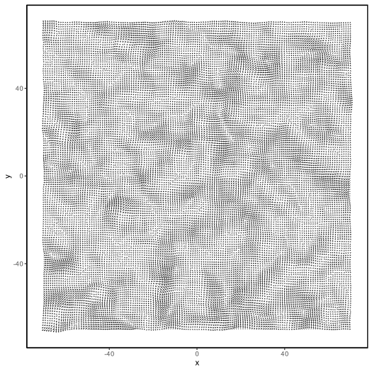
Figure B.1: An example of a simulated wind field, where x and y are coordinates in metres. Vectors are derived from the simulated u and v components. Vector lengths are in m s^-1 and scaled by a factor of 0.10.

Appendix C Appendix: simulation results

Table 1: Confusion matrix denoting the precision rate (bold diagonal; $true.state/(true.state+false.state$) and the false discovery rate (off-diagonal; $false.state/(true.state+false.state$) of the simulated 500 steps as predicted by the CRW HMM and BCRW HMM. Values denote the mean and [2.5%, 97.5%] quantiles across the 100 simulated tracks.

			Simulated state
			D	O	ARS
Predicted state	CRW HMM	D	0.37 [0.35, 0.39]	0.01 [0.00, 0.02]	0.09 [0.06, 0.11]
		O	0.06 [0.05, 0.07]	0.95 [0.93, 0.96]	0.00 [0.00, 0.01]
		ARS	0.57 [0.55, 0.59]	0.04 [0.04, 0.05]	0.91 [0.89, 0.93]
	BCRW HMM	D	0.97 [0.97, 0.98]	0.00 [0.00, 0.00]	0.06 [0.06, 0.07]
		O	0.00 [0.00, 0.00]	0.99 [0.98, 0.99]	0.01 [0.01, 0.01]
		ARS	0.03 [0.02, 0.03]	0.01 [0.01, 0.02]	0.93 [0.93, 0.94]

See pages 1-13 of Tutorial.pdf

References

- Adam et al. (2019) Adam, T., Griffiths, C.A., Meese, E.N., Lowe, C.G., Blackwell, P.G., Righton, D. & Langrock, R. (2019). Joint modelling of multi-scale animal movement data using hierarchical hidden Markov models. Methods in Ecology and Evolution, 2019, 1536–1550. http://dx.doi.org/10.1111/2041-210X.13241
- Arrieta et al. (2017) Arrieta, J., Barreira, A., Chioccioli, M., Polin, M. & Tuval, I. (2017). Phototaxis beyond turning: Persistent accumulation and response acclimation of the microalga Chlamydomonas reinhardtii. Scientific Reports, 7(1), 1–7. http://dx.doi.org/10.1038/s41598-017-03618-8
- Auger-Méthé et al. (2016a) Auger-Méthé, M., Derocher, A.E., DeMars, A.C., Plank, J.M., Codling, E.A. & Lewis, M.A. (2016a). Evaluating random search strategies in three mammals from distinct feeding guilds. mathualbertaca, 85, 1411–1421. http://dx.doi.org/10.1111/1365-2656.12562
- Auger-Méthé et al. (2015) Auger-Méthé, M., Derocher, A.E., Plank, M.J., Codling, E.A. & Lewis, M.A. (2015). Differentiating the Lévy walk from a composite correlated random walk. Methods in Ecology and Evolution, 6(10), 1179–1189. http://dx.doi.org/10.1111/2041-210X.12412
- Auger-Méthé et al. (2016b) Auger-Méthé, M., Lewis, M.A. & Derocher, A.E. (2016b). Home ranges in moving habitats: Polar bears and sea ice. Ecography, 39(1), 26–35. http://dx.doi.org/10.1111/ecog.01260
- Bai et al. (2015) Bai, X., Hu, H., Wang, J., Yu, Y., Cassano, E. & Maslanik, J. (2015). Responses of surface heat flux, sea ice and ocean dynamics in the Chukchi-Beaufort sea to storm passages during winter 2006/2007: A numerical study. Deep-Sea Research Part I: Oceanographic Research Papers, 102, 101–117. http://dx.doi.org/10.1016/j.dsr.2015.04.008
- Bailey et al. (2018) Bailey, J.D., Wallis, J. & Codling, E.A. (2018). Navigational efficiency in a biased and correlated random walk model of individual animal movement. Ecology, 99(1), 217–223. http://dx.doi.org/10.1002/ecy.2076
- Baker et al. (2018) Baker, K.L., Dickinson, M., Findley, T.M., Gire, D.H., Louis, M., Suver, M.P., Verhagen, J.V., Nagel, K.I. & Smear, M.C. (2018). Algorithms for olfactory search across species. Journal of Neuroscience, 38(44), 9383–9389. http://dx.doi.org/10.1523/JNEUROSCI.1668-18.2018
- Bartumeus et al. (2016) Bartumeus, F., Campos, D., Ryu, W.S., Lloret-Cabot, R., Méndez, V. & Catalan, J. (2016). Foraging success under uncertainty: search tradeoffs and optimal space use. Ecology Letters, 19(11), 1299–1313. http://dx.doi.org/10.1111/ele.12660
- Benhamou (2006) Benhamou, S. (2006). Detecting an orientation component in animal paths when the preferred direction is individual-dependent. Ecology, 87(2), 518–528. http://dx.doi.org/10.1890/05-0495
- Benhamou (2014) Benhamou, S. (2014). Of scales and stationarity in animal movements. Ecology Letters, 17(3), 261–272. http://dx.doi.org/10.1111/ele.12225
- Bestley et al. (2013) Bestley, S., Jonsen, I.D., Hindell, M.A. & Guinet, C. (2013). Integrative modelling of animal movement : incorporating in situ habitat and behavioural information for a migratory marine predator. Proceedings of the Royal Society B, 280(1750), 20122262. http://dx.doi.org/http://dx.doi.org/10.1098/rspb.2012.2262
- Blanchet et al. (2020) Blanchet, M.A., Aars, J., Andersen, M. & Routti, H. (2020). Space-use strategy affects energy requirements in Barents Sea polar bears. Marine Ecology Progress Series, 639, 1–19. http://dx.doi.org/10.3354/meps13290
- Bracis & Mueller (2017) Bracis, C. & Mueller, T. (2017). Memory, not just perception, plays an important role in terrestrial mammalian migration. Proceedings of the Royal Society B: Biological Sciences, 284(1855), 20170449. http://dx.doi.org/10.1098/rspb.2017.0449
- Chambellant et al. (2012) Chambellant, M., Lunn, N.J. & Ferguson, S.H. (2012). Temporal variation in distribution and density of ice-obligated seals in western Hudson Bay, Canada. Polar Biology, 35(7), 1105–1117. http://dx.doi.org/10.1007/s00300-012-1159-6
- Codling & Bode (2016) Codling, E.A. & Bode, N.W. (2016). Balancing direct and indirect sources of navigational information in a leaderless model of collective animal movement. Journal of Theoretical Biology, 394, 32–42. http://dx.doi.org/10.1016/j.jtbi.2016.01.008
- Codling et al. (2008) Codling, E.A., Plank, M.J. & Benhamou, S. (2008). Random walk models in biology. Journal of the Royal Society Interface, 5(25), 813–834. http://dx.doi.org/10.1098/rsif.2008.0014
- Derocher (2021) Derocher, A.E. (2021). Replication Data for: Togunov RR, Derocher AE, Lunn NJ, Auger-Méthé M. 2021. Characterising menotatic behaviours in movement data using hidden Markov models. Methods in Ecology and Evolution. QYMAYV, UAL Dataverse. http://dx.doi.org/10.7939/DVN/QYMAYV
- Diego-Rasilla & Luengo (2004) Diego-Rasilla, F.J. & Luengo, R.M. (2004). Heterospecific call recognition and phonotaxis in the orientation behavior of the marbled newt, Triturus marmoratus. Behavioral Ecology and Sociobiology, 55(6), 556–560. http://dx.doi.org/10.1007/s00265-003-0740-y
- Dohan & Maximenko (2010) Dohan, K. & Maximenko, N. (2010). Monitoring ocean currents with satellite sensors. Oceanography, 23(4), 94–103. http://dx.doi.org/10.5670/oceanog.2010.08
- Duchesne et al. (2015) Duchesne, T., Fortin, D. & Rivest, L.P. (2015). Equivalence between step selection functions and biased correlated random walks for statistical inference on animal movement. PLoS ONE, 10(4), e0122947. http://dx.doi.org/10.1371/journal.pone.0122947
- Fagan et al. (2013) Fagan, W.F., Lewis, M.A., Auger-Méthé, M., Avgar, T., Benhamou, S., Breed, G., Ladage, L., Schlägel, U.E., Tang, W.W., Papastamatiou, Y.P., Forester, J. & Mueller, T. (2013). Spatial memory and animal movement. Ecology Letters, 16(10), 1316–1329. http://dx.doi.org/10.1111/ele.12165
- Florko et al. (2020) Florko, K.R., Thiemann, G.W. & Bromaghin, J.F. (2020). Drivers and consequences of apex predator diet composition in the Canadian Beaufort Sea. Oecologia, 1, 3. http://dx.doi.org/10.1007/s00442-020-04747-0
- Gaspar et al. (2006) Gaspar, P., Georges, J.Y., Fossette, S., Lenoble, A., Ferraroli, S. & Le Maho, Y. (2006). Marine animal behaviour: Neglecting ocean currents can lead us up the wrong track. Proceedings of the Royal Society B: Biological Sciences, 273(1602), 2697–2702. http://dx.doi.org/10.1098/rspb.2006.3623
- Gaynor et al. (2019) Gaynor, K.M., Brown, J.S., Middleton, A.D., Power, M.E. & Brashares, J.S. (2019). Landscapes of Fear: Spatial Patterns of Risk Perception and Response. http://dx.doi.org/10.1016/j.tree.2019.01.004
- Goto et al. (2017) Goto, Y., Yoda, K. & Sato, K. (2017). Asymmetry hidden in birds’ tracks reveals wind, heading, and orientation ability over the ocean. Science Advances, 3(9), e1700097. http://dx.doi.org/10.1126/sciadv.1700097
- Hersbach et al. (2020) Hersbach, H., Bell, B., Berrisford, P., Hirahara, S., Horányi, A., Muñoz‐Sabater, J., Nicolas, J., Peubey, C., Radu, R., Schepers, D., Simmons, A., Soci, C., Abdalla, S., Abellan, X., Balsamo, G., Bechtold, P., Biavati, G., Bidlot, J., Bonavita, M., Chiara, G. & et al. (2020). The ERA5 global reanalysis. Quarterly Journal of the Royal Meteorological Society, 146(730), 1999–2049. http://dx.doi.org/10.1002/qj.3803
- Hijmans & van Etten (2016) Hijmans, R.J. & van Etten, J. (2016). Package “raster”. Geographic data analysis and modeling. pp. 1–242.
- Johnson & London (2018) Johnson, D.S. & London, J.M. (2018). crawl: an R package for fitting continuous-time correlated random walk models to animal movement data. pp. 1–30.
- Johnson et al. (2008) Johnson, D.S., London, J.M., Lea, M.A. & Durban, J.W. (2008). Continuous-time correlated random walk model for animal telemetry data. Ecology, 89(5), 1208–1215. http://dx.doi.org/10.1890/07-1032.1
- Kays et al. (2015) Kays, R., Crofoot, M.C., Jetz, W. & Wikelski, M. (2015). Terrestrial animal tracking as an eye on life and planet. Science, 348(6240), 2478–1. http://dx.doi.org/10.1126/science.aaa2478
- Kennedy & Marsh (1974) Kennedy, J.S. & Marsh, D. (1974). Pheromone-regulated anemotaxis in flying moths. Science, 184(4140), 999–1001. http://dx.doi.org/10.1126/science.184.4140.999
- Klappstein et al. (2020) Klappstein, N.J., Togunov, R.R., Reimer, J.R., Lunn, N.J. & Derocher, A.E. (2020). Patterns of ice drift and polar bear (Ursus maritimus) movement in Hudson Bay. Marine Ecology Progress Series, 641, 227–240. http://dx.doi.org/10.3354/meps13293
- Langrock et al. (2012) Langrock, R., King, R., Matthiopoulos, J., Thomas, L., Fortin, D., Morales, J.M. & Angrock, R. (2012). Flexible and practical modeling of animal telemetry data: hidden Markov models and extensions. Ecology, 93(11), 2336–2342. http://dx.doi.org/10.1890/11-2241.1
- Lohmann et al. (2008) Lohmann, K.J., Lohmann, C.M. & Endres, C.S. (2008). The sensory ecology of ocean navigation. Journal of Experimental Biology, 211(11), 1719–1728. http://dx.doi.org/10.1242/jeb.015792
- Lunn et al. (2016) Lunn, N.J., Servanty, S., Regehr, E.V., Converse, S.J., Richardson, E.S. & Stirling, I. (2016). Demography of an apex predator at the edge of its range: impacts of changing sea ice on polar bears in Hudson Bay. Ecological Applications, 26(5), 1302–1320. http://dx.doi.org/10.1890/15-1256
- Mauritzen et al. (2003) Mauritzen, M., Derocher, A.E., Pavlova, O. & Wiig, Ø. (2003). Female polar bears, Ursus maritimus, on the Barents Sea drift ice: Walking the treadmill. Animal Behaviour, 66(1), 107–113. http://dx.doi.org/10.1006/anbe.2003.2171
- McClintock et al. (2012) McClintock, B.T., King, R., Thomas, L., Matthiopoulos, J., Mcconnell, B. & Morales, J.M. (2012). A general discrete-time modeling framework for animal movement using multistate random walks. Ecological Monographs, 82(3), 335–349. http://dx.doi.org/10.1890/11-0326.1
- McClintock et al. (2020) McClintock, B.T., Langrock, R., Gimenez, O., Cam, E., Borchers, D.L., Glennie, R. & Patterson, T.A. (2020). Uncovering ecological state dynamics with hidden Markov models. Ecology Letters, 23(12), 1878–1903. http://dx.doi.org/10.1111/ele.13610
- McClintock & Michelot (2018) McClintock, B.T. & Michelot, T. (2018). momentuHMM: R package for generalized hidden Markov models of animal movement. Methods in Ecology and Evolution, 9(6), 1518–1530. http://dx.doi.org/10.1111/2041-210X.12995
- Mestre et al. (2014) Mestre, F., Bragança, M.P., Nunes, A. & dos Santos, M.E. (2014). Satellite tracking of sea turtles released after prolonged captivity periods. Marine Biology Research, 10(10), 996–1006. http://dx.doi.org/10.1080/17451000.2013.872801
- Michelot et al. (2017) Michelot, T., Langrock, R., Bestley, S., Jonsen, I.D., Photopoulou, T. & Patterson, T.A. (2017). Estimation and simulation of foraging trips in land-based marine predators. Ecology, 98(7), 1932–1944. http://dx.doi.org/10.1002/ecy.1880
- Mouritsen (2018) Mouritsen, H. (2018). Long-distance navigation and magnetoreception in migratory animals. Nature, 558(7708), 50–59. http://dx.doi.org/10.1038/s41586-018-0176-1
- Nagy et al. (2010) Nagy, M., Ákos, Z., Biro, D. & Vicsek, T. (2010). Hierarchical group dynamics in pigeon flocks. Nature, 464(7290), 890–893. http://dx.doi.org/10.1038/nature08891
- Nevitt et al. (2008) Nevitt, G.A., Losekoot, M. & Weimerskirch, H. (2008). Evidence for olfactory search in wandering albatross, Diomedea exulans. Proceedings of the National Academy of Sciences, 105(12), 4576–4581. http://dx.doi.org/10.1073/pnas.0709047105
- Paiva et al. (2010) Paiva, V.H., Guilford, T., Meade, J., Geraldes, P., Ramos, J.A. & Garthe, S. (2010). Flight dynamics of Cory’s shearwater foraging in a coastal environment. Zoology, 113(1), 47–56. http://dx.doi.org/10.1016/j.zool.2009.05.003
- Park & Lee (2017) Park, J.H. & Lee, H.S. (2017). Phototactic behavioral response of agricultural insects and stored-product insects to light-emitting diodes (LEDs). Applied Biological Chemistry, 60(2), 137–144. http://dx.doi.org/10.1007/s13765-017-0263-2
- Patterson et al. (2008) Patterson, T.A., Thomas, L., Wilcox, C., Ovaskainen, O. & Matthiopoulos, J. (2008). State–space models of individual animal movement. Trends in Ecology and Evolution, 23(2), 87–94. http://dx.doi.org/10.1016/j.tree.2007.10.009
- Pilfold et al. (2012) Pilfold, N.W., Derocher, A.E., Stirling, I., Richardson, E.S. & Andriashek, D. (2012). Age and sex composition of seals killed by polar bears in the Eastern Beaufort sea. PLoS ONE, 7(7), e41429. http://dx.doi.org/10.1371/journal.pone.0041429
- Potts et al. (2014) Potts, J.R., Auger-Méthé, M., Mokross, K. & Lewis, M.A. (2014). A generalized residual technique for analysing complex movement models using earth mover’s distance. Methods in Ecology and Evolution, 5(10), 1012–1022. http://dx.doi.org/10.1111/2041-210X.12253
- R Core Team (2020) R Core Team (2020). R: A language and environment for statistical computing.
- Rivest & Duchesne (2016) Rivest, L.p. & Duchesne, T. (2016). A general angular regression model for the analysis. Applied Statistics, 65(3), 445–463.
- Roever et al. (2014) Roever, C.L., Beyer, H.L., Chase, M.J. & Van Aarde, R.J. (2014). The pitfalls of ignoring behaviour when quantifying habitat selection. Diversity and Distributions, 20(3), 322–333. http://dx.doi.org/10.1111/ddi.12164
- Safi et al. (2013) Safi, K., Kranstauber, B., Weinzierl, R., Griffin, L., Rees, E.C., Cabot, D., Cruz, S., Proaño, C., Takekawa, J.Y., Newman, S.H., Waldenström, J., Bengtsson, D., Kays, R., Wikelski, M. & Bohrer, G. (2013). Flying with the wind: scale dependency of speed and direction measurements in modelling wind support in avian flight. Movement Ecology, 1(1), 1–4. http://dx.doi.org/10.1186/2051-3933-1-4
- Savoca et al. (2017) Savoca, M.S., Tyson, C.W., McGill, M. & Slager, C.J. (2017). Odours from marine plastic debris induce food search behaviours in a forage fish. Proceedings of the Royal Society B: Biological Sciences, 284(1860), 20171000. http://dx.doi.org/10.1098/rspb.2017.1000
- Schick et al. (2008) Schick, R.S., Loarie, S.R., Colchero, F., Best, B.D., Boustany, A., Conde, D.A., Halpin, P.N., Joppa, L.N., McClellan, C.M. & Clark, J.S. (2008). Understanding movement data and movement processes: Current and emerging directions. Ecology Letters, 11(12), 1338–1350. http://dx.doi.org/10.1111/j.1461-0248.2008.01249.x
- Smith & Stirling (1975) Smith, T.G. & Stirling, I. (1975). The breeding habitat of the ringed seal (Phoca hispida). The birth lair and associated structures. Canadian Journal of Zoology, 53(9), 1297–1305. http://dx.doi.org/10.1139/z75-155
- Stirling (1974) Stirling, I. (1974). Midsummer observations on the behavior of wild polar bears (Ursus maritimus). Canadian Journal of Zoology, 52(9), 1191–1198. http://dx.doi.org/10.1139/z74-157
- Stirling & Latour (1978) Stirling, I. & Latour, P.B. (1978). Comparative hunting abilities of polar bear cubs of different ages. Canadian Journal of Zoology, 56(8), 1768–1772. http://dx.doi.org/10.1139/z78-242
- Stirling & McEwan (1975) Stirling, I. & McEwan, E.H. (1975). The caloric value of whole ringed seals (Phoca hispida) in relation to polar bear (Ursus maritimus) ecology and hunting behavior. Canadian journal of zoology, 53(8), 1021–1027. http://dx.doi.org/10.1139/z75-117
- Stirling et al. (1989) Stirling, I., Spencer, C. & Andriashek, D.S. (1989). Immobilization of polar bears (Ursus maritimus) with Telazol ® in the Canadian Arctic. Journal of Wildlife Diseases, 25(2), 159–168. http://dx.doi.org/10.7589/0090-3558-25.2.159
- Stirling et al. (2016) Stirling, I., Spencer, C. & Andriashek, D. (2016). Behavior and activity budgets of wild breeding polar bears (Ursus maritimus). Marine Mammal Science, 32(1), 13–37. http://dx.doi.org/10.1111/mms.12291
- Togunov et al. (2017) Togunov, R.R., Derocher, A.E. & Lunn, N.J. (2017). Windscapes and olfactory foraging in a large carnivore. Scientific Reports, 7, 46332. http://dx.doi.org/10.1038/srep46332
- Togunov et al. (2018) Togunov, R.R., Derocher, A.E. & Lunn, N.J. (2018). Corrigendum: Windscapes and olfactory foraging in a large carnivore (Scientific Reports DOI: 10.1038/srep46332). Scientific Reports, 8, 46968. http://dx.doi.org/10.1038/srep46968
- Togunov et al. (2021) Togunov, R.R., Derocher, A.E., Lunn, N.J. & Auger-Méthé, M. (2021). Replication Code for: Characterising menotactic behaviours in movement data using hidden Markov models. http://dx.doi.org/10.5281/zenodo.5070812
- Togunov et al. (2020) Togunov, R.R., Klappstein, N.J., Lunn, N.J., Derocher, A.E. & Auger-Méthé, M. (2020). Opportunistic evaluation of modelled sea ice drift using passively drifting telemetry collars in Hudson Bay, Canada. The Cryosphere, 14(6), 1937–1950. http://dx.doi.org/10.5194/tc-2020-26
- Tschudi et al. (2010) Tschudi, M.A., Fowler, C.W., Maslanik, J.A. & Stroeve, J. (2010). Tracking the movement and changing surface characteristics of Arctic sea ice. IEEE Journal of Selected Topics in Applied Earth Observations and Remote Sensing, 3(4), 536–540. http://dx.doi.org/10.1109/JSTARS.2010.2048305
- Ventura et al. (2020) Ventura, F., Granadeiro, J.P., Padget, O. & Catry, P. (2020). Gadfly petrels use knowledge of the windscape, not memorized foraging patches, to optimize foraging trips on ocean-wide scales. Proceedings of the Royal Society B: Biological Sciences, 287(1918), 20191775. http://dx.doi.org/10.1098/rspb.2019.1775
- Ware et al. (2017) Ware, J.V., Rode, K.D., Bromaghin, J.F., Douglas, D.C., Wilson, R.R., Regehr, E.V., Amstrup, S.C., Durner, G.M., Pagano, A.M., Olson, J., Robbins, C.T. & Jansen, H.T. (2017). Habitat degradation affects the summer activity of polar bears. Oecologia, 184(1), 87–99. http://dx.doi.org/10.1007/s00442-017-3839-y
- Wilmers et al. (2015) Wilmers, C.C., Nickel, B., Bryce, C.M., Smith, J.A., Wheat, R.E., Yovovich, V. & Hebblewhite, M. (2015). The golden age of bio-logging: How animal-borne sensors are advancing the frontiers of ecology. Ecology, 96(7), 1741–1753. http://dx.doi.org/10.1890/14-1401.1
- Wilson et al. (2012) Wilson, R.R., Gilbert-Norton, L. & Gese, E.M. (2012). Beyond use versus availability: behaviour-explicit resource selection. Wildlife Biology, 18(4), 424–430. http://dx.doi.org/10.2981/12-044
- Ylitalo et al. (2020) Ylitalo, A.K., Heikkinen, J. & Kojola, I. (2020). Analysis of central place foraging behaviour of wolves using hidden Markov models. Ethology, 127(2), 145–157. http://dx.doi.org/10.1111/eth.13106
- Yonehara et al. (2016) Yonehara, Y., Goto, Y., Yoda, K., Watanuki, Y., Young, L.C., Weimerskirch, H., Bost, C.A. & Sato, K. (2016). Flight paths of seabirds soaring over the ocean surface enable measurement of fine-scale wind speed and direction. Proceedings of the National Academy of Sciences, 113(32), 9039–9044. http://dx.doi.org/10.1073/pnas.1523853113
- Yu et al. (2020) Yu, X., Rinke, A., Dorn, W., Spreen, G., Lüpkes, C., Sumata, H. & Gryanik, V.M. (2020). Evaluation of Arctic sea ice drift and its dependency on near-surface wind and sea ice conditions in the coupled regional climate model HIRHAM-NAOSIM. The Cryosphere, 14(5), 1727–1746. http://dx.doi.org/10.5194/tc-14-1727-2020
- Zucchini et al. (2016) Zucchini, W., MacDonald, I.L. & Langrock, R. (2016). Hidden Markov Models for Time Series. Taylor & Francis, Boca Raton, second edition.