HD 183579b: A Warm Sub-Neptune Transiting a Solar Twin Detected by TESS

Abstract

We report the discovery and characterization of a transiting warm sub-Neptune planet around the nearby bright ($V=8.75$ mag, $K=7.15$ mag) solar twin HD 183579, delivered by the Transiting Exoplanet Survey Satellite (TESS). The host star is located $56.8\pm 0.1$ pc away with a radius of $R_{\ast}=0.97\pm 0.02\ R_{\odot}$ and a mass of $M_{\ast}=1.03\pm 0.05\ M_{\odot}$. We confirm the planetary nature by combining space and ground-based photometry, spectroscopy, and imaging. We find that HD 183579b (TOI-1055b) has a radius of $R_{p}=3.53\pm 0.13\ R_{\oplus}$ on a $17.47$ day orbit with a mass of $M_{p}=11.2\pm 5.4\ M_{\oplus}$ ($3\sigma$ mass upper limit of $27.4\ M_{\oplus}$). HD 183579b is the fifth brightest known sub-Neptune planet system in the sky, making it an excellent target for future studies of the interior structure and atmospheric properties. By performing a line-by-line differential analysis using the high resolution and signal-to-noise ratio HARPS spectra, we find that HD 183579 joins the typical solar twin sample, without a statistically significant refractory element depletion.

1 Introduction

After the first discovery of a hot Jupiter outside our Solar system (Mayor & Queloz, 1995), exoplanet research has moved into a new era. Up to now, more than 4 000 exoplanets have been confirmed . Most giant planets have been found by successful ground surveys like HATNet (Bakos et al., 2004), SuperWASP (Pollacco et al., 2006), KELT (Pepper et al., 2007; Pepper et al., 2012) and NGTS (Chazelas et al., 2012; Wheatley et al., 2018). Space mission conducting photometric transit surveys including CoRoT (Baglin et al., 2006), Kepler (Borucki et al., 2010) and K2 (Howell et al., 2014) have led to the further detections of thousands of planets with size between Earth and Neptune. These diverse exoplanets are hosted by a similarly diverse set of stars. Among them, Sun-like stars (here defined as FGK main-sequence stars) make up a significant fraction of known planet hosts. These systems can be seen as an intriguing opportunity to get a glimpse into alternate paths to that our own Solar system might have taken in its early formation, and they represent our best opportunity to discover a “truly Earth-like” exoplanet that exists under conditions as similar as possible to our own planet (Horner et al., 2020; Kane et al., 2021).

Solar twins are an important subset of Sun-like stars. Typically defined by their extreme similarity to the Sun in fundamental spectroscopic properties ($T_{\rm eff}$ within 100 K, $\log g$ within 0.1 dex, and [Fe/H] within 0.1 dex of Solar values), these stars must by definition have such similar photospheric conditions to the Sun so that their spectra can be directly compared with minimal reliance on stellar atmospheric models. The result of a line-by-line differential spectroscopic analysis of a solar twin yields uniquely precise abundance measurements for the star and thereby for the star-planet system (see e.g. Bedell et al., 2018; Spina et al., 2018, who achieve 0.01 dex or 2% precision on abundance measurements for over 30 elements). This is in direct contrast to a typical planet host star, whose abundances are expected to be limited by systematic uncertainties to the level of 0.05 dex or more. Similarly precise measurements may be made of the star’s age, mass, radius, and other fundamental properties by combining isochronal models with the spectroscopic measurements (Ramírez et al., 2014; Yana Galarza et al., 2016). It is worth emphasizing that these properties are measured with extreme precision (not necessarily accuracy) relative to the Sun, our most thoroughly characterized planet host. Planetary systems around solar twin stars are therefore useful both as individual well-characterized planets but also as a prime sample for comparative studies delving into any subtle differences between stars that host planets of different types. Unfortunately, the sample of solar twins with well characterized planets around is still limited in number at present (e.g., Kepler-11, Lissauer et al. 2011; HIP 11915, Bedell et al. 2015; K2-231, Curtis et al. 2018; KELT-22, Labadie-Bartz et al. 2019), roughly 50 in total.

The Transiting Exoplanet Survey Satellite (TESS, Ricker et al. 2014, 2015), which performs an all-sky survey and focuses on small exoplanets orbiting nearby bright stars, will likely increase the sample of planets around solar twins significantly (Sullivan et al., 2015; Huang et al., 2018). During its two-year primary mission, TESS has detected over two thousand exoplanet candidates, the majority of which are suitable for follow-up observations, including mass measurements and atmospheric spectroscopy. This makes TESS planet candidates unlike most Kepler systems, which are too faint for these follow-up observation.

In this work, we present a warm sub-Neptune planet detected by TESS to orbit a solar twin star HD 183579. HD 183579 is a G2V star with a spectrum nearly identical to that of the Sun. The star has been studied extensively through a dedicated RV planet search and spectroscopic abundance survey targeting solar twin stars with the High Accuracy Radial velocity Planet Searcher spectrograph (HARPS, Mayor et al. 2003; Meléndez et al. 2015). The transiting planet, however, was not detected until TESS data became available.

This paper is organized as follows: In Section 2, we describe all observations. We characterize the host star HD 183579 in Section 3. Section 4 presents our analysis of the light curves and RV data. The lessons about comparison between HD 183579 and other similar systems are discussed in Section 5. In Section 6, we discuss insights into this system, prospects for further characterization via transmission spectroscopy, a search for additional planets, and a comparison with a recently published analysis of archival RVs of this target (Palatnick et al., 2021). We conclude our findings in Section 7.

2 Observations

2.1 TESS

HD 183579 (TIC 320004517) was monitored by TESS with the two-minute cadence mode in Sector 13 during the primary mission and Sector 27 during the extended mission. The data were obtained between 2019 June 19th and 2019 July 18th, and between 2020 July 5th and 2020 July 30th, consisting of a total of 20479 and 17546 individual measurements, respectively.

The raw images were reduced using the Science Processing Operations Center (SPOC) pipeline (Jenkins et al., 2016), which was developed at NASA Ames Research Center based on the Kepler mission’s science pipeline. After the systematic and dilution effects were corrected by the Presearch Data Conditioning (PDC; Stumpe et al. 2012; Smith et al. 2012; Stumpe et al. 2014) module, Transiting Planet Search (TPS; Jenkins, 2002; Jenkins et al., 2017) was then performed to look for transit-like signals. HD 183579 was finally identified as a planet candidate in the TESS Object of Interest catalog (TOI 1055.01) with a period of 17.47 days and a transit depth of 1259 ppm (Twicken et al., 2018; Li et al., 2019), and alerted on the MIT TESS Alerts portal.

We downloaded the Presearch Data Conditioning Simple Aperture Photometry (PDCSAP) light curve from the Mikulski Archive for Space Telescopes (MAST). After removing all measurements flagged for quality issues in SPOC to improve the precision, we applied the built-in routines of the lightkurve package (Lightkurve Collaboration et al., 2018; Barentsen et al., 2019) to normalize the data and clip outliers above a $+5\sigma$ limit. These additional processing steps removed 904 and 802 points (4.4% and 4.6%), with 19575 and 16744 measurements left for each sector.

To search for potential additional planets, we smoothed the light curve with a median filter and performed an independent transit search using the Box Least Square (BLS; Kovács et al. 2002) algorithm. We confirmed the $\sim 17$ d signal reported by TPS. Except for that, we did not detect any other significant peaks existing in the periodogram.

After masking out all in-transit data, we detrended the light curve by fitting a Gaussian Process (GP) model with a simple Matern32 kernel using the celerite package (Foreman-Mackey et al., 2017). Figure 1 shows the original SAP, PDCSAP and the PDCSAP light curve after detrending. We used this reprocessed light curve in our further transit analysis.

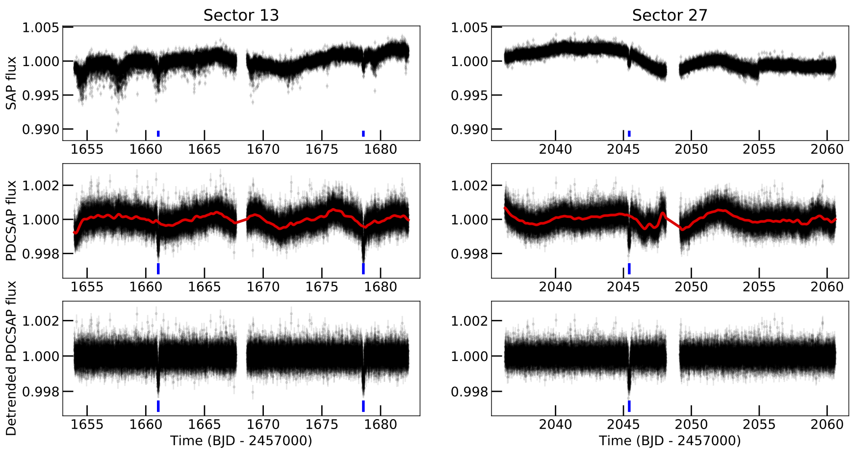
Figure 1: Top panels: The original TESS SAP light curves of HD 183579 from Sector 13 and 27. Middle panels: The PDCSAP light curves of HD 183579 along with the best-fit GP model shown as red solid lines. Bottom panels: The detrended PDCSAP light curves. The three transits of HD 183579b are marked in blue ticks.

2.2 Ground-Based Photometry

2.2.1 Las Cumbres Observatory (LCO)

The large pixel scale of TESS ($21^{\prime\prime}$ per pixel, Ricker et al. 2014, 2015) may result in light contamination from stars close to the target, making nearby eclipsing binaries (NEB) a common source of TESS false positives (Brown, 2003; Sullivan et al., 2015). To rule out the NEB scenario and confirm the event on target, we collected two ground-based follow-up observations using the Las Cumbres Observatory Global Telescope (LCOGT) network (Brown et al., 2013). We used the TESS Transit Finder (TTF), which is a customized version of the Tapir software package (Jensen, 2013), to schedule these time-series observations. The photometric observations were taken in the Pan-STARRS $Y$ band with an exposure time of 35 s on 2020 June 27th and 2020 August 1st at Siding Spring Observatory (SSO), Australia and both were done with 1m telescopes. The Sinistro cameras have a $26^{\prime}\times 26^{\prime}$ field of view as well as a plate scale of $\rm 0.389^{\prime\prime}$ per pixel. The images were defocused and have stellar point-spread-functions (PSF) with a full-width-half-maximum (FWHM) of $\sim 2\aas@@fstack{\prime\prime}4$ and $\sim 2\aas@@fstack{\prime\prime}0$, respectively. After the images were calibrated by the standard automatic BANZAI pipeline (McCully et al., 2018), we carried out photometric analysis using AstroImageJ (Collins et al. 2017). We excluded all nearby stars within 1 arcmin as the source causing the TESS signal with brightness difference down to $\Delta T\sim 7.5$ mag (see Figure 2), and confirmed the signal on target. We summarize the observations in Table 1.

Table 1: Summary of ground-based photometric observations for HD 183579

Facility	Date	Total exposures	Exposure time(s)	Filter	Coverage	Label
LCO 1m SSO Sinistro	2020 June 27	224	35	Pan-STARRS $Y$	egress	LCOA
LCO 1m SSO Sinistro	2020 Aug 1	274	35	Pan-STARRS $Y$	egress	LCOB

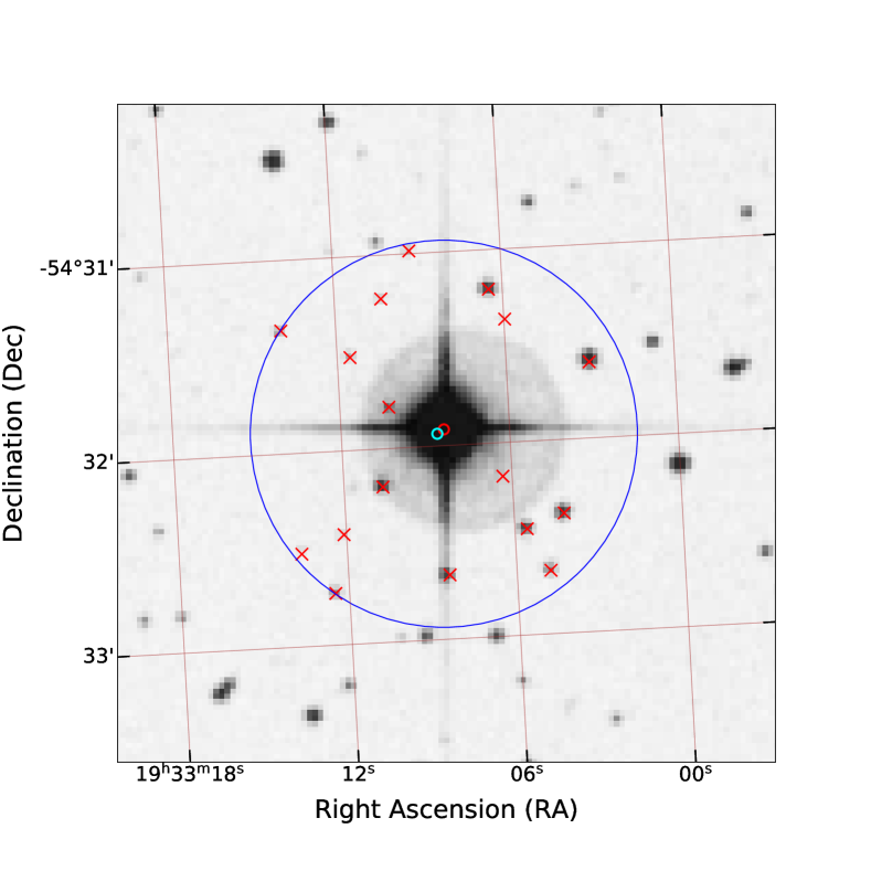
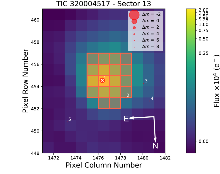
Figure 2: Left panel: The POSS2 blue image of HD 183579 taken in 1976. The center red dot is the target star in this image and the cyan dot shows its current position. All stars (marked as red crosses) in 1^′ (the blue circle) are ruled out as the source that causes the TESS detection based on their brightness and the NEB analysis of LCO photometry. Right panel: Target pixel file (TPF) of HD 183579 in TESS Sector 13 (created with tpfplotter, Aller et al. (2020)). Different sizes of red circles represent different magnitudes in contrast with HD 183579 ($\Delta m$). The red-square region represents the aperture used to extract the photometry by SPOC. The light contamination from nearby stars is negligible (see Section 4.1).

2.2.2 WASP

WASP-South, an array of 8 cameras, was the Southern half of the WASP transit-search survey (Pollacco et al., 2006). The field of HD 183579 was observed in both 2013 and 2014, covering a span of 180 nights in each year with a typical 10-min cadence on clear nights, and accumulating 52 000 data points. WASP-South was equipped with 85-mm, f/1.2 lenses giving a photometric extraction aperture with a 112-arcsec radius. All other stars within this aperture are $>$ 5 mag fainter.

2.3 High Resolution Spectroscopy

2.3.1 HARPS

HD 183579 was observed 56 times by the High Accuracy Radial velocity Planet Searcher (HARPS; Mayor et al. 2003) on the ESO 3.6 m telescope at La Silla Observatory in Chile between 2011 and 2019. The bulk of these observations were made as part of a dedicated blind planet search targeting solar twins (P.I. Meléndez). All observations were carried out in high-accuracy mode with a spectral resolution R $\sim$ 115,000. The median SNR is 108 pix^-1 at 600 nm.

We extracted the radial velocity (RV) measurements, chromatic RV index (CRX) and differential line width (dLW) using the publicly available SpEctrum Radial Velocity AnaLyser pipeline (SERVAL, Zechmeister et al. 2018). Additional diagnostics including the inverse bisector span (BIS) and full width at half-maximum (FWHM) for the line profile of the average spectral features were extracted by the standard HARPS pipeline using a cross-correlation technique with a solar-type mask (Pepe et al., 2002). These diagnostics are commonly used as stellar activity tracers, since they quantify the line distortions which mimic Doppler shifts.

In addition to these activity indicators, we also derived the $S_{\rm HK}$ measurement, which quantifies the strength of emission in the cores of the Ca II H&K lines. These were measured and corrected to the standard Mount Wilson scaling using the procedure outlined in Lovis et al. (2011). Measured $S_{\rm HK}$ values and photon-noise-based uncertainties along with the pipeline values of RV, BIS, FWHM, CRX and dLW are publicly available on ExoFOP-TESS.

We dropped one observation (BJD=2457588.767) from the analysis because its BIS and FWHM measurements were significant outliers ($>5\sigma$) from the general distribution, pointing to potential issues with the data reduction and RV extraction.

2.3.2 Minerva-Australis

Minerva-Australis is an array of four PlaneWave CDK700 telescopes located at the Mt Kent Observatory in Queensland, Australia, fully dedicated to the precise radial-velocity follow-up of TESS candidates (e.g. Jordán et al., 2020; Addison et al., 2021, 2020). The four telescopes can be simultaneously fiber-fed to a single KiwiSpec R4-100 high-resolution (R=80,000) spectrograph (Barnes et al., 2012; Addison et al., 2019). HD 183579 was monitored by Minerva-Australis using up to 4 telescopes in the array between 2020 April 19 and 2020 June 1. Each epoch consists of one or two 30-minute exposures. Telescopes 1, 3, 4, and 5 (denoted as MA, MB, MC and MD) obtained 5, 8, 15, and 5 epochs respectively. Radial velocities for the observations are derived for each telescope by cross-correlation, where the template being matched is the mean spectrum of each telescope. A simultaneous quartz-illuminated iodine cell in the calibration fibres provides the wavelength calibration and corrects for instrumental variations. We converted all time-stamps of our measurements from JD to BJD using barycorr (Wright & Eastman, 2014).

2.4 High Angular Resolution Imaging

High-angular resolution imaging is needed to search for nearby sources that can contaminate the TESS photometry, resulting in an underestimated planetary radius, or other sources of astrophysical false positives, such as background eclipsing binaries.

2.4.1 Gemini-South

We observed HD 183579 to probe for companion stars on 12 September 2019 UT using the Zorro instrument mounted on the 8 m Gemini South telescope, located on Cerro Pachón in Chile. Zorro uses speckle imaging to simultaneously observe diffraction-limited images at 562 nm (0.017^′′) and 832 nm (0.028^′′). Our data set consisted of three $1000\times 60$ ms exposure images simultaneously obtained in both band-passes, followed by a single $1000\times 60$ ms image, also in both band-passes, of a PSF standard star.

Following the procedures outlined in Howell et al. (2011), we combined all images and subjected them to Fourier analysis, and produce re-constructed imagery from which 5-sigma contrast curves are derived in each passband (Figure 3). Our data reveal HD 183579 to be a single star to contrast limits of 5 to 8 magnitudes within the spatial limits of 1.0/1.6 AU (562/832 nm respectively) out to 57 AU.

2.4.2 SOAR

We also searched for stellar companions to HD 183579 with speckle imaging on the 4.1-m Southern Astrophysical Research (SOAR) telescope (Tokovinin, 2018) on 31 October 2020 UT, observing in Cousins I-band, a similar visible bandpass as TESS. More details of the observations are available in Ziegler et al. (2020). The 5$\sigma$ detection sensitivity and speckle auto-correlation functions from the observations are shown in the right panel of Figure 3. No nearby stars were detected within 3″of HD 183579 in the SOAR observations.

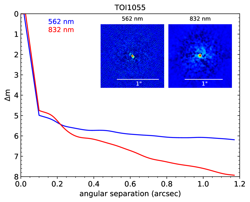
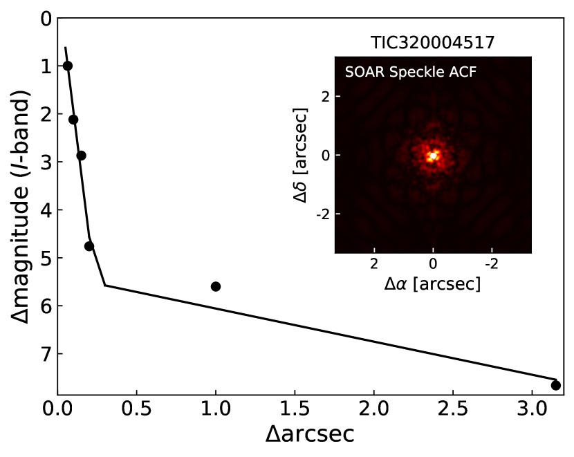
Figure 3: Left panel: Zorro speckle imaging and $5\sigma$ contrast curves of HD 183579 at 562 nm and 832 nm. The data reveal that no companion star is detected within the spatial limits of 1 AU out to 57 AU with a $\Delta$ m of 5 to 8. Right panel: Speckle ACF obtained in the I band using SOAR. The 5$\sigma$ contrast curve for HD 183579 is shown by the black points. Black solid line corresponds to the linear fit of the data, at separations smaller and larger than $\sim 0.2^{\prime\prime}$.

3 Stellar properties

3.1 Stellar Characterization

We first derived $T_{\rm eff}$, $R_{\ast}$, and iron abundance [Fe/H] from the spectroscopic data. By utilizing the SpecMatch-Emp package (Yee et al., 2017), we matched the co-added HARPS spectrum to a high resolution spectroscopic library, which contains 404 well-characterized stars, following Hirano et al. (2018). We found $T_{\rm eff}=5678\pm 110$ K, $R_{\ast}=0.988\pm 0.100\ R_{\odot}$ and ${\rm[Fe/H]}=-0.07\pm 0.09$ dex. This is in good agreement with the literature values of $T_{\rm eff}=5798\pm 4$ K, $\log g=4.480\pm 0.012$ dex, and ${\rm[Fe/H]}=-0.036\pm 0.003$ dex, as derived by Spina et al. (2018) using the same co-added HARPS observations with a strictly differential line-by-line equivalent width technique.

For comparison, we then performed an analysis of the broadband spectral energy distribution (SED) together with the Gaia EDR3 parallax (Gaia Collaboration et al., 2021) in order to determine an empirical measurement of the stellar radius, following the procedures described in Stassun & Torres (2016) and Stassun et al. (2017); Stassun et al. (2018a). We gathered the FUV, NUV magnitudes from GALEX (Morrissey et al., 2007), the $B_{\rm T}$, $V_{\rm T}$ magnitudes from Tycho-2 (Høg et al., 2000), the Strömgren $u$,$v$,$b$,$y$ magnitudes from Paunzen (2015), the $J$,$H$,$K_{S}$ magnitudes from 2MASS Point Source Catalog (Cutri et al., 2003; Skrutskie et al., 2006), four Wide-field Infrared Survey Explorer (WISE) magnitudes (Wright et al., 2010) and three Gaia magnitudes $G$, $G_{\rm BP}$, $G_{\rm RP}$. Together, the available photometry spans the full stellar SED over the wavelength range 0.15–22 $\mu$m (see Figure 4).

We performed a fit using the Kurucz stellar atmosphere models, with the priors on effective temperature ($T_{\rm eff}$), surface gravity ($\log g$) and metallicity ([Fe/H]) from the spectroscopic analysis. The remaining free parameter is the extinction ($A_{V}$), which we limited to the maximum permitted for the star’s line of sight from the dust maps (Schlegel et al., 1998). The best-fit SED is shown in Figure 4 with a reduced $\chi^{2}=1.4$ (excluding the GALEX UV measurements, which indicate mild chromospheric activity; see below) and $A_{V}=0.01\pm 0.01$. Integrating the model SED gives a bolometric flux at Earth of $F_{\rm bol}=9.32\pm 0.11\times 10^{-9}$ erg s^-1 cm^-2. Taking the $F_{\rm bol}$ and $T_{\rm eff}$ together with the Gaia parallax, we obtained a stellar radius of $R_{\ast}=0.972\pm 0.014\ R_{\odot}$, which agrees with the previous result within $1\sigma$.

We computed an empirical estimate of the stellar mass from this $R_{\ast}$ together with the spectroscopic $\log g$, from which we obtained $M_{\ast}=1.03\pm 0.05\ M_{\odot}$. This is consistent with that estimated via the eclipsing-binary based relations of Torres et al. (2010), which gives $M_{\ast}=1.04\pm 0.06\ M_{\odot}$.

Taking all the results above into consideration, we finally adopted the weighted mean values of effective temperature $T_{\rm eff}$, stellar radius $R_{\ast}$ and stellar mass $M_{\ast}$. Combining the expected stellar radius with mass, we found a mean stellar density of $\rm\rho_{\ast}=1.58\pm 0.16$ g cm^-3.

Following Johnson & Soderblom (1987), we adopted the astrometric values ($\varpi$, $\mu_{\alpha}$, $\mu_{\delta}$) from Gaia EDR3 (Gaia Collaboration et al., 2021) as well as systemic RV taken from Gaia DR2 (Gaia Collaboration et al., 2018), and computed the three-dimensional Galactic space motion of ($U_{\rm LSR}$, $V_{\rm LSR}$, $W_{\rm LSR}$) = ($-23.10\pm 0.19$, $1.53\pm 0.06$, $-14.14\pm 0.10$) km s^-1, all of which are relative to the LSR. Building on the kinematic calculation, we then determined the relative probability $P_{\rm thick}/P_{\rm thin}$ of HD 183579 to be in the thick and thin disks (Bensby et al., 2003; Bensby et al., 2014). We obtained $P_{\rm thick}/P_{\rm thin}=0.01$, indicating a thin-disk origin. We further employed the galpy package (Bovy, 2015) to estimate the maximal height $Z_{\rm max}$ of HD 183579 above the Galactic plane, along with the “MWPotential2014” Galactic potential following Gan et al. (2020). We find HD 183579 has a $Z_{\rm max}$ of $\sim 213$ pc, which agrees with our thin-disk conclusion.

The GALEX photometry suggests a mild amount of chromospheric activity. Indeed, Lorenzo-Oliveira et al. (2018) reported a spectroscopically measured $\log R^{\prime}_{\rm HK}=-4.89\pm 0.02$, consistent with a mild level of activity. Based on the Yonsei-Yale isochrones, Spina et al. (2018) found that HD 183579 has an age of $2.6\pm 0.5$ Gyr. We list all final adopted stellar parameter values in Table 2.

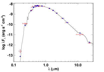
Figure 4: The best SED fit for HD 183579. The Red symbols show the observed photometric measurements, where the horizontal bars represent the effective width of the passband. The Blue points are the predicted integrated fluxes at the corresponding bandpass. The black line represents the best-fit NextGen atmosphere model.

Table 2: Stellar parameters of HD 183579

Parameter	Value	Reference
Star ID
TIC	320004517
TOI	1055
HIP	96160
Astrometric properties
$\alpha\ (J2000)$	19:33:08.58
$\delta\ (J2000)$	$-$54:31:56.50
$\varpi$ (mas)	$17.609\pm 0.016$	Gaia EDR3
$\mu_{\alpha}$ (mas yr-1)	$108.32\pm 0.01$	Gaia EDR3
$\mu_{\delta}$ (mas yr-1)	$-82.71\pm 0.01$	Gaia EDR3
RV (km s-1)	$-15.8\pm 0.2$	Gaia DR2
Photometric properties
${\it TESS}$ (mag)	$8.089\pm 0.006$	$\rm TIC\ V8^{[1]}$
$G$ (mag)	$8.5265\pm 0.0002$	Gaia EDR3
$G_{\rm BP}$ (mag)	$8.843\pm 0.001$	Gaia EDR3
$G_{\rm RP}$ (mag)	$8.037\pm 0.002$	Gaia EDR3
$B_{T}$ (mag)	$9.477\pm 0.019$	Tycho-2
$V_{T}$ (mag)	$8.750\pm 0.013$	Tycho-2
$J$ (mag)	$7.518\pm 0.023$	2MASS
$H$ (mag)	$7.231\pm 0.047$	2MASS
$K_{S}$ (mag)	$7.150\pm 0.027$	2MASS
$W1$ (mag)	$7.090\pm 0.043$	WISE
$W2$ (mag)	$7.137\pm 0.020$	WISE
$W3$ (mag)	$7.138\pm 0.019$	WISE
$W4$ (mag)	$7.040\pm 0.114$	WISE
Derived parameters
$\log g_{\ast}$ (cgs)	$4.47\pm 0.03$	This work
$\rm[Fe/H]$ (dex)	$-0.07\pm 0.09$	This work
Distance (pc)	$56.79\pm 0.06$	This work
$U_{\rm LSR}$ (km s-1)	$-23.10\pm 0.19$	This work
$V_{\rm LSR}$ (km s-1)	$1.53\pm 0.06$	This work
$W_{\rm LSR}$ (km s-1)	$-14.14\pm 0.10$	This work
$T_{\rm eff}^{[2]}$ (K)	$5706\pm 110$	This work
$M_{\ast}\ (M_{\odot})$	$1.034\pm 0.050$	This work
$R_{\ast}\ (R_{\odot})$	$0.974\pm 0.015$	This work
$\rm\rho_{\ast}\ (g~{}cm^{-3})$	$1.58\pm 0.16$	This work
$P_{\rm rot}$ (day)	$23.2\pm 3.7$	This work
$A_{V}$ (mag)	$0.01\pm 0.01$	This work
Age (Gyr)	$2.6\pm 0.5$	Spina et al. (2018)

• [1] Stassun et al. (2018b, 2019)

• [2] We take the average values of $T_{\rm eff}$, $M_{\ast}$ and $R_{\ast}$ here (see Section 3.1).

3.2 Stellar Rotation

The TESS PDCSAP light curve from sector 13 shows a clear variation with a timescale of $\sim 9.5$ d, which implies a relatively high stellar rotation speed. However, this periodic signature is not shown in the corresponding SAP light curve (see Figure 1). Additionally, the subsequent light curve from the extended mission does not have a similar trend. We show below that this $\sim 9.5$ d signal is more likely due to instrumental systematic errors instead of real stellar variability.

First, we estimated the rotation period $P_{\rm rot}/\sin i=24.4\pm 2.6$ d based on the stellar radius $R_{\ast}$ together with the spectroscopically determined rotational velocity $v\sin i=2.1\pm 0.2$ km s^-1 (Soto & Jenkins, 2018). Assuming $\sin i=1$, this is consistent with the value $P_{\rm rot}=23.2\pm 3.7$ d inferred using the empirical activity-rotation relation from Mamajek & Hillenbrand (2008) according to gyrochronology (Barnes, 2007; Meibom et al., 2009; Curtis et al., 2019).

Furthermore, McQuillan et al. (2014) analyzed the rotation periods of main-sequence stars below 6500 K based on three years of data from the Kepler space mission. Our derived rotation period $P_{\rm rot}$ $23.2\pm 3.7$ d of HD 183579 agrees with the typical value $\sim 20$ d of solar-like stars with a $T_{\rm eff}$ of $\sim 5700$ K (see Figures 4 and 5 in McQuillan et al. 2014).

We also investigated the rotational modulation in the WASP accumulated data as archival long term light curve could provide information on stellar rotation features. However, we did not find significant signals likely due to the influence of lunar stray light in the 23-27 d regime.

Finally, we performed a frequency analysis for the HARPS activity indicators (CRX, dLW, bisector span, FWHM and $S_{\rm HK}$). One instrumental effect must be accounted for here: In June 2015, the HARPS optical fibers were replaced as part of a major instrument upgrade, leaving an effective offset between RVs and other line profile-sensitive components measured before and after the upgrade (Lo Curto et al., 2015). For this initial inspection, we calculated the median values for both RVs and each indicator, and subtracted the corresponding offset between pre-upgrade and post-upgrade data. Because of the sparse sampling, we did not see any significant periodic signals, therefore, we do not present the periodograms here. However, we found strong correlations between RVs and CRX, dLW and FWHM ($r=-0.41$, p-value $=2\times 10^{-3}$; $r=0.42$, p-value $=1\times 10^{-3}$; $r=0.41$, p-value $=2\times 10^{-3}$) and weak correlations between RVs and $S_{\rm HK}$ ($r=0.26$, p-value $=0.06$) as shown in Figure 5, which motivated us to take the stellar activity into consideration in the following RV modeling (see Section 4.2).

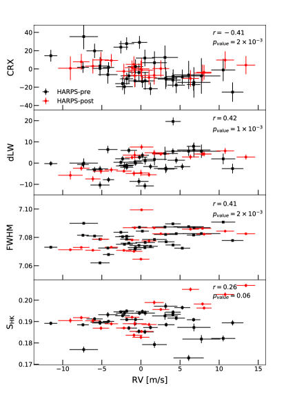
Figure 5: Correlations between HARPS RVs and activity indicators (CRX, dLW, FWHM and $S_{\rm HK}$). Different colors represent HARPS pre-upgrade/post-upgrade data. The Pearson’s correlation indices and the corresponding p-values are shown on the upper right. In each plot we have subtracted the median value of both RV and the activity indices. The clear correlations indicate that stellar activity has an effect on the Doppler signals (see Section 3.2).

4 Analysis

4.1 Photometric Analysis

We utilized the juliet package (Espinoza et al., 2019) to perform a joint-fit of both space and ground-based light curves. The transit is modeled by batman (Kreidberg, 2015). We applied the dynamic nested sampling approach to determine the posterior probability distribution of the system parameters using the public package dynesty (Higson et al., 2019; Speagle, 2020).

We retrieved a list of nearby stars of HD 183579 ($G_{\rm rp}=8.037$ mag) within 30^′′ in Gaia EDR3 to estimate the flux dilution effect in the ground-based photometries (Espinoza et al., 2019). Three faint stars with $G_{\rm rp}>17.4$ mag are found located at $>25^{\prime\prime}$ away from HD 183579. As the nearby stars are faint and relatively distant, these stars should make minor contribution to the contaminated flux, which is consistent with the small contamination ratio $A_{D}=0.001$ reported in the TESS Input Catalog (TIC) V8 (Stassun et al., 2018b, 2019). Thus we fixed the dilution factors $D_{\rm LCO}$ equal to 1 but considered individual instrument offsets.

We adopted Gaussian priors for the period $P_{b}$ and mid-transit time $t_{0}$ based on the results from the Box Least Square search. juliet applies the new parametrizations $r_{1}$ and $r_{2}$ to sample points (Espinoza, 2018), for which we set uniform priors between 0 and 1. We adopted a quadratic limb-darkening law for TESS photometry and uniformly sampled the coefficients ($q_{1}$ and $q_{2}$, Kipping 2013). For ground-based data, we used a linear law instead to parameterize the limb-darkening effect and placed a Gaussian prior on the coefficient, centered at the theoretical estimate derived from the LDTK package (Husser et al., 2013; Parviainen & Aigrain, 2015) with a $1\sigma$ value of 0.1. We fit a circular orbit for HD 183579b with a non-informative log-uniform prior set on the stellar density. For each instrument, we included a flux jitter term to account for the white noise. The results of the fit along with the corresponding prior settings are listed in Table 3. We present the best-fit models in Figure 6.

Table 3: Model parameters, prior settings and the best-fit values for the TESS and ground-based light curves of HD 183579.

Parameter	Best-fit Value	Prior	Description
Planetary parameters
$P_{b}$ (days)	$17.47128^{+0.00005}_{-0.00005}$	$\mathcal{N}^{[1]}$ ($17.4$ , $0.1^{2}$)	Orbital period of HD 183579b.
$T_{0,b}$ (BJD-2457000)	$1661.06295^{+0.00070}_{-0.00071}$	$\mathcal{N}$ ($1661.1$ , $0.1^{2}$)	Mid-transit time of HD 183579b.
$r_{1,b}$	$0.613^{+0.133}_{-0.127}$	$\mathcal{U}^{[2]}$ (0 , 1)	Parametrisation for p and b.
$r_{2,b}$	$0.03319^{+0.00069}_{-0.00056}$	$\mathcal{U}$ (0 , 1)	Parametrisation for p and b.
$e_{b}$	0	Fixed	Orbital eccentricity of HD 183579b.
$\omega_{b}$ (deg)	90	Fixed	Argument of periapsis of HD 183579b.
TESS photometry parameters
$D_{\rm TESS}$	$1$	Fixed	TESS photometric dilution factor.
$M_{\rm TESS}$	$-0.0000003^{+0.000002}_{-0.000002}$	$\mathcal{N}$ (0 , $0.1^{2}$)	Mean out-of-transit flux of TESS photometry.
$\sigma_{\rm TESS}$ (ppm)	$110^{+5}_{-5}$	$\mathcal{J}^{[3]}$ ($10^{-6}$ , $10^{6}$)	TESS additive photometric jitter term.
$q_{1}$	$0.32^{+0.18}_{-0.12}$	$\mathcal{U}$ (0 , 1)	Quadratic limb darkening coefficient.
$q_{2}$	$0.26^{+0.32}_{-0.17}$	$\mathcal{U}$ (0 , 1)	Quadratic limb darkening coefficient.
LCOA photometry parameters
$D_{\rm LCOA}$	$1$	Fixed	LCOA photometric dilution factor.
$M_{\rm LCOA}$	$-0.0006^{+0.00008}_{-0.00007}$	$\mathcal{N}$ (0 , $0.1^{2}$)	Mean out-of-transit flux of LCOA photometry.
$\sigma_{\rm LCOA}$ (ppm)	$520^{+147}_{-234}$	$\mathcal{J}$ ($0.1$ , $10^{5}$)	LCOA additive photometric jitter term.
$q_{\rm LCOA}$	$0.42^{+0.07}_{-0.09}$	$\mathcal{N}$ ($0.37$ , $0.1^{2}$)	Linear limb darkening coefficient.
LCOB photometry parameters
$D_{\rm LCOB}$	$1$	Fixed	LCOB photometric dilution factor.
$M_{\rm LCOB}$	$-0.0006^{+0.00008}_{-0.00008}$	$\mathcal{N}$ (0 , $0.1^{2}$)	Mean out-of-transit flux of LCOB photometry.
$\sigma_{\rm LCOB}$ (ppm)	$817^{+87}_{-85}$	$\mathcal{J}$ ($0.1$ , $10^{5}$)	LCOB additive photometric jitter term.
$q_{\rm LCOB}$	$0.35^{+0.09}_{-0.08}$	$\mathcal{N}$ ($0.37$ , $0.1^{2}$)	Linear limb darkening coefficient.
Stellar parameters
${\rho}_{\ast}$ ($\rm kg\ m^{-3}$)	$1514^{+353}_{-535}$	$\mathcal{J}$ ($100$ , $\rm 100^{2}$)	Stellar density.
Derived parameters
$R_{p}/R_{\ast}$	$0.03319^{+0.00069}_{-0.00056}$		Planet radius in units of stellar radii.
$R_{p}$ ($R_{\oplus}$)	$3.53^{+0.13}_{-0.11}$		Planet radius.
${b}$	$0.42^{+0.20}_{-0.19}$		Impact Parameter.
$a/R_{\ast}$	$29.0^{+2.1}_{-2.8}$		Semi-major axis in units of stellar radii.
$a$ (AU)	$0.13^{+0.01}_{-0.01}$		Semi-major axis.
$i$ (deg)	$89.17^{+0.40}_{-0.58}$		Inclination angle.
$T_{\rm eq}^{[4]}$ (K)	$748^{+55}_{-40}$		Equilibrium temperature.

• [1] $\mathcal{N}$($\mu\ ,\ \sigma^{2}$) means a normal prior with mean $\mu$ and standard deviation $\sigma$.

• [2] $\mathcal{U}$(a ,  b) stands for a uniform prior ranging from a to b.

• [3] $\mathcal{J}$(a ,  b) stands for a Jeffrey’s prior ranging from a to b.

• [4] We assume there is no heat distribution between the dayside and nightside, and that the albedo is zero.

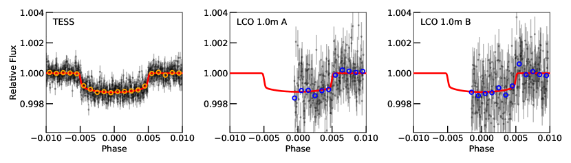
Figure 6: Phase-folded transits of HD 183579b for all available photometric instruments. TESS data are presented in the left panel. Two LCO 1m/Sinistro light curves obtained in the Pan-STARRS Y band are shown in the middle and right panels. The orange and blue points represent the binned light curves. The best-fit models are shown as red solid lines.

4.2 RV modeling

We chose to fit the RVs independently of the transit fit with priors informed by the photometric analysis. We employed the forecaster package to predict the mass of HD 183579b (Chen & Kipping, 2017). We obtained $12.0^{+9.0}_{-5.3}\ M_{\oplus}$ based on the probabilistic mass-radius relation, which corresponds to a radial velocity semi-amplitude $K_{b}$ of $\sim 2.8^{+2.2}_{-1.2}$ m/s, assuming a circular orbit. This expected RV signal is beyond the detection capability of Minerva (typical error bar is $\sim 7$ m/s). Hence, we chose to analyze the HARPS-only data set first to avoid the Minerva RVs obscuring the signal, then combine the additional Minerva data and perform a joint-fit.

4.2.1 HARPS-only

We fit the HARPS-only RVs independent of the transit modeling with priors coming from the best-fit transit ephemeris. Juliet utilizes the radvel algorithm to create the Keplerian model (Fulton et al., 2018) for the RV time series data. We compared different RV models based on the Bayesian model log-evidence ($\ln Z$) calculated by the dynesty package. In general, a model is favoured if $\Delta\ln Z>2$ compared with the other, and strongly supported if $\Delta\ln Z>5$ (Trotta, 2008).

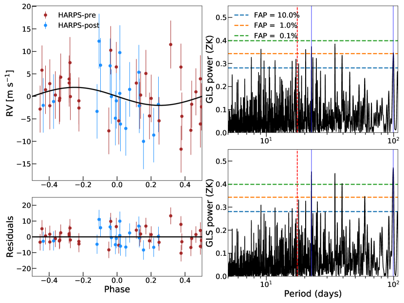
Figure 7: Top left panel: The phase-folded HARPS RVs of HD 183579. The best-fit base model is shown as a black solid line. Bottom left panel: RV residuals after subtracting the best-fit Keplerian model. The error bars are the quadrature sum of the instrument jitter term and the measurement uncertainties for all RVs. Right panels: The GLS periodograms of the total HARPS RV data (top) and the residuals (bottom) after adjusting for the RV offsets between different instruments using the best-fit values from our base model. The 10%, 1% and 0.1% FAP levels are shown as horizontal dashed lines. The red vertical dashed line represents the period of HD 183579b ($P_{b}=17.47$ d) derived from the light curve fit. The periodogram of the RV residuals shows up a forest of peaks between 22.6 d and 99.2 d (two blue vertical lines) which may be due to the stellar activity (see Section 4.2).

We first performed a simple 1-planet (i.e. HD 183579b) Keplerian orbit fit with uniform priors on $e\sin\omega$ and $e\cos\omega$. We treated the HARPS-pre and HARPS-post data as from two different instruments and included the RV offset and the RV jitter terms for each set of data. We obtained $e=0.49\pm 0.30$, indicating the current RVs are insufficient to constrain the eccentricity. Moreover, compared with a circular orbit model, we found the Bayesian evidence is not significantly stronger for the eccentric model ($\Delta\ln Z=\ln Z_{\rm ecc}-\ln Z_{\rm circ}<1$). Thus we chose to fix the orbital eccentricity to 0 in all our runs and considered this 1-planet circular orbit model as our base model (hereafter BM; 1pl). We further compared the $\ln Z$ of the BM model and a no-planet model (np), and we found a significant improvement ($\Delta\ln Z=\ln Z_{\rm BM}-\ln Z_{\rm np}=13$), supporting the existence of the planet. The BM model gives $K_{b}=2.3^{+1.1}_{-1.0}$ m/s, which leads to a marginal mass measurement of $9.5\pm 4.5\ M_{\oplus}$. We show all HARPS RV data along with best-fit model in Figure 7. The RV periodogram does not show an obvious planet signal at $\sim 17$ d or any other significant peaks with $\rm FAP<0.1\%$ due to the poor sampling. However, subtracting the best-fit BM model resulted in a forest of peaks between 22.6 d and 99.2 d with $\rm FAP<0.1\%$ in the GLS periodogram of residuals, which may arise from additional planets in the system or from noise that was not accounted for in our model (e.g. stellar activity).

To investigate the source of these new peaks we identified in the GLS periodogram (see Figure 7), we fit a BM+1pl (HD 183579b + a potential outer planet) model, allowing the period $P_{c}$ vary uniformly between 20 d and 110 d along with a wide uniform prior on the RV semi-amplitude $K_{c}$. However, we did not find any convergences in the $P_{c}-K_{c}$ space, indicating that there is no evidence for the existence of another outer non-transiting planet within the period range. This is also confirmed by the Bayesian model log-evidence, which only shows a negligible improvement compared with the BM model ($\Delta\ln Z=\ln Z_{\rm BM+1pl}-\ln Z_{\rm BM}=2$).

If stellar activity signals are present in the data, from surface features rotating across the star or from longer-term variations in the net convective blueshift suppression, they could also add peaks to the periodogram. In particular, the phase incoherence of activity signals due to constantly-evolving surface features over the long duration of RV observations will contribute excess power in disordered structures around the rotation period and its harmonics, which unfortunately coincide with the region of period space we wish to search. With all of this in mind, we explored two approaches to deal with the stellar activity effect on the Doppler signals.

First, we modeled the RVs using Gaussian Process regression (BM+GP) with an quasi-periodic kernel formulated by Foreman-Mackey et al. (2017):

$$k_{i,j}(\tau)=\frac{B}{2+C}e^{-\tau/L}\left[{\rm cos}\left(\frac{2\pi\tau}{P_{\rm rot}}\right)+(1+C)\right],$$ (1)

where $B$ defines the GP covariance amplitude, $C$ is a balance parameter for the periodic and the non-periodic parts, $\tau=|t_{i}-t_{j}|$ is the time-lag between data point $i$ and $j$. $L$ and $P_{\rm rot}$ represent the coherence timescale and the stellar rotational period, respectively. We adopted uninformative, wide log-uniform priors to the GP parameters except for the periodic timescale $P_{\rm rot}$, where we chose a narrow Gaussian prior centering at 23.2 d with $\sigma_{P_{\rm rot}}=4$ d according to our findings in Section 3.2. We obtained $K_{b}=4.3\pm 1.0$ m/s, which is consistent with our estimate from BM+1pl within $2\sigma$. Although we noticed a significant enhancement of $\ln Z$ ($\Delta\ln Z=\ln Z_{\rm BM+GP}-\ln Z_{\rm BM}=8$), we suspected the GP model might have over-fitted the RV data. The expected stellar rotation timescale ($\sim 23$ d) is much smaller than the total RV baseline ($>2800$ d) and the current RV data points are too sparse, which implies the stellar activity signal is not well sampled, making GP not robust in such a challenging case. Comparing with a GP-only model, we also found a $\ln Z$ improvement of the BM+GP model ($\Delta\ln Z=\ln Z_{\rm BM+GP}-\ln Z_{\rm GP}=5$).

We then constructed a simple and fast-to-compute model by involving the activity indicators into the analysis (BM+FWHM). We first tested this option by checking to see whether accounting for activity indicators via linear correlations in the RV analysis would reduce the RV noise to the point that the planet signal could be seen in the periodogram. We adopted a linear relationship between RV and the HARPS FWHM, which was previously shown to correlate significantly with RV (Figure 5). We also added in a quadratic trend component to account for long-term changes in the RVs due to either the evolving magnetic activity cycle or undetected long-period companions. With this more advanced model, we constructed a log-likelihood periodogram. This approach is a simple and efficient way of searching frequency space while taking certain systematic noise sources into account, and follows the methodology behind the Systematics-Insensitive Periodogram introduced for Kepler transit searches by Angus et al. (2016). It is analogous to the Bayesian Generalized Lomb-Scargle periodogram introduced by Mortier et al. (2015), but contains additional noise terms. Specifically, in our application the model prediction is that for any time $t_{n}$ with corresponding FWHM measurement $w_{n}$, the RV $y_{n}$ is given by:

$$\begin{split}y_{n}=&ax_{n}^{2}+bx_{n}+c_{n}+dw_{n}+K\sin\Big{(}\frac{2\pi}{P}t_{n}\Big{)}+\\ &H\cos\Big{(}\frac{2\pi}{P}t_{n}\Big{)}+\mathrm{noise},\end{split}$$ (2)

where $x_{n}$ is a normalized relative time:

$$x_{n}=\frac{t_{n}-\langle\mathbf{t}\rangle}{\mathrm{max}(\mathbf{t})-\mathrm{min}(\mathbf{t})},$$ (3)

the baseline term $c_{n}$ is comprised of two possible values based on whether observation $n$ was taken before or after HARPS upgrade time $t_{\rm upgrade}$:

$$c_{n}=c_{1}\delta_{n}+c_{2}\neg\delta_{n},$$ (4)

with $\delta_{n}$ set to 1 for pre-upgrade data and 0 for post-upgrade data. The variables ($a,b,c_{1},c_{2},d,K,H,P$) are unknowns to be constrained from the data. At any given value of the orbital period $P$, this model is entirely linear, so that the vector of predicted RVs $\mathbf{y}$ can be calculated as a product of a design matrix

$$\mathbf{A_{P}}=\begin{pmatrix}x_{0}^{2}&x_{0}&\delta_{0}&\neg\delta_{0}&w_{0}&\sin\Big{(}\frac{2\pi}{P}t_{0}\Big{)}&\cos\Big{(}\frac{2\pi}{P}t_{0}\Big{)}\\ \vdots&\vdots&\vdots&\vdots&\vdots&\vdots&\vdots\\ x_{n}^{2}&x_{n}&\delta_{n}&\neg\delta_{n}&w_{n}&\sin\Big{(}\frac{2\pi}{P}t_{n}\Big{)}&\cos\Big{(}\frac{2\pi}{P}t_{n}\Big{)}\end{pmatrix}$$ (5)

and a variable vector

$$\mathbf{\Theta}=[a,b,c_{1},c_{2},d,K,H]^{T}.$$ (6)

At the period $P_{b}$, then, the optimal parameters $\mathbf{\Theta^{*}_{P}}$ can be analytically determined as the following:

$$\mathbf{\Theta^{*}_{P}}=(\mathbf{A_{P}}^{\mathsf{T}}\mathbf{C}^{-1}\mathbf{A_{P}})^{-1}\mathbf{A_{P}}^{\mathsf{T}}\mathbf{C}^{-1}\mathbf{y},$$ (7)

where $\mathbf{C}^{-1}$ is the covariance matrix for the data, here assumed to be diagonal. We stepped through a log-uniform grid of periods between 1 and 1000 days and determine the maximum likelihood for each period (neglecting a constant term):

$$\mathrm{ln}\mathcal{L}^{*}_{P}\sim-\frac{1}{2}(\mathbf{y}-\mathbf{A_{P}}\mathbf{\Theta^{*}_{P}})^{\mathsf{T}}\mathbf{C}^{-1}(\mathbf{y}-\mathbf{A_{P}}\mathbf{\Theta^{*}_{P}}).$$ (8)

The resulting log-likelihood periodogram shares the fundamental assumption of a circular orbit but is otherwise more robust to stellar activity and long-period trends than a traditional Lomb-Scargle periodogram (Lomb, 1976; Scargle, 1982). Due to the linearity of the model and the resulting ability to find the optimal parameters analytically, the likelihood may be maximized quickly and with a guarantee of convexity. Therefore, while more advanced tools exist to incorporate Bayesian priors (Olspert et al., 2018) or non-parametric correlated noise (Feng et al., 2017) along with trends in the data, this method is relatively simple to implement, flexible, and fast, making it a practical solution for RV planet searches carried out in the presence of non-negligible stellar noise. The log-likelihood periodogram does show a strong peak at 17 days (Figure 8). We show the resulting fit in Figure 9. While this supports the presence of a sinusoidal, potentially Keplerian signal in the data, we note that this conclusion depends on the noise model adopted. The 17-day peak is the highest in the log-likelihood periodogram, but a forest of other strong peaks remain. In brief, the above analysis shows that the RV data do support the detection of a 17-day planet, but the signal is not sufficiently strong or robust to changes in the noise model to confidently claim detection on the grounds of RVs alone.

The results of the log-likelihood periodogram experiment motivated us to include an RV-FWHM correlation term in the RV model (BM+FWHM). We implemented this model fit using pymc3 and the exoplanet package (Salvatier et al., 2016; Foreman-Mackey et al., 2020). The parameterization and priors adopted were identical those used in the juliet analysis, with the addition of two free parameters: the slope of the linear correlation between RV and FWHM, $S_{\rm FWHM}$, and an offset of the post-HARPS-upgrade FWHM measurements with respect to the pre-upgrade FWHMs, $\Delta_{\rm FWHM}$. Both of these parameters received broad and uninformative Gaussian priors.

We regard this BM+FWHM model as our final best model because (1) The BM+FWHM model yields constraints on the planet parameters that are in full agreement with the BM model (Figure 9, Table 4); (2) The BM+FWHM takes stellar activity into consideration while the BM model does not. Though including the FWHM term reduces the white-noise jitter slightly, it is an insignificant reduction, which suggests that the source of the excess noise in the HARPS RV measurements is not sufficiently captured by a FWHM correlation. More RV observations taken with denser sampling to preserve coherency of the stellar activity signal may be necessary to improve the noise model.

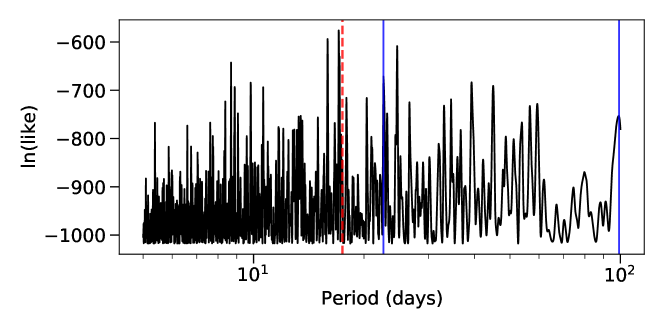
Figure 8: Periodogram of the HARPS RVs employing the log-likelihood periodogram method described in the text. Vertical lines mark the period of HD 183579b (red dashed line) and the bounds of the forest of peaks seen in Figure 7 (blue solid lines). After accounting for a linear correlation between RV and FWHM and including a quadratic background term, the noise is suppressed to the extent that a 17-day peak can be seen.

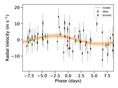
Figure 9: Phase-folded radial velocities for HD 183579b using the BM+FWHM fit. Individual data points and their photon-noise-based uncertainties are shown as black points and error bars, while the grey error bars represent the uncertainties inflated by the best-fit (posterior median) jitter parameters. Green points are the error-weighted means within a series of phase bins. The best-fit BM+FWHM model is shown as a solid orange line, with the shaded region around it marking the model’s $1\sigma$ credible interval.

4.2.2 Including the Minerva data

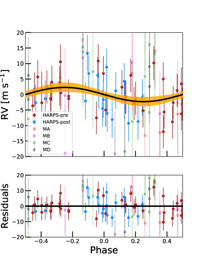
Figure 13: The phase-folded HARPS and Minerva RVs of HD 183579. The best-fit base model is shown as a black solid line. The orange shaded region represents the $1\sigma$ confidence interval of the model. Residuals are plotted below.

We finally re-ran a Keplerian fit after including the Minerva-Australis RVs. As HD 183579 is monitored by four telescopes (Minerva 1, 3, 4 and 5; denoted as MA, MB, MC and MD) in the array, we treated each data set separately and fit individual offsets and jitters, but kept the same prior settings for other parameters as in Section 4.2.1. We obtained $K_{b}=2.2^{+1.0}_{-0.9}$ m/s, which corresponds to a mass of $9.2^{+4.1}_{-3.7}\ M_{\oplus}$ with a $3\sigma$ upper limit of $21.7\ M_{\oplus}$, estimated using the 99.7% value of $K_{b}$ in the posterior distribution. This measurement is consistent with the estimate from the HARPS-only data analysis within $1\sigma$. We list our final results in Table 4 and show the best-fit model of all data in Figure 13. As the Minerva data were noisy with low cadence, we did not attempt to use them to fit the stellar activity.

Table 4: Parameters, prior settings and the best-fit values for the HD 183579 system of three models

Parameter	Priors	BM for HARPS	BM+FWHM for HARPS	BM for HARPS+Minerva
Planetary parameters
$P_{b}$ (days)	$\mathcal{N}$ ($17.47128$ , $0.00005^{2}$)	$17.47129^{+0.00004}_{-0.00004}$	$17.4712750^{+0.0000097}_{-0.0000153}$	$17.47128^{+0.00005}_{-0.00004}$
$T_{0,b}$ (BJD)	$\mathcal{N}$ ($2458661.0628$ , $0.0007^{2}$)	$2458661.06279^{+0.00050}_{-0.00051}$	$2458661.06279^{+0.00071}_{-0.00069}$	$2458661.06279^{+0.00054}_{-0.00054}$
$e_{b}$	Fixed	0	0	0
$\omega_{b}$ (deg)	Fixed	90	90	90
RV offset
$\rm\mu_{HARPS_{pre}}$ ($\rm m\ s^{-1}$)	$\mathcal{U}$ ($-10$ , $10$)	$0.64^{+0.89}_{-0.88}$	$0.9^{+0.9}_{-0.9}$	$0.65^{+0.90}_{-0.90}$
$\rm\mu_{HARPS_{post}}$ ($\rm m\ s^{-1}$)	$\mathcal{U}$ ($-10$ , $10$)	$1.28^{+1.33}_{-1.35}$	$0.7^{+6.5}_{-5.6}$	$1.30^{+1.32}_{-1.33}$
$\rm\mu_{MA}$ ($\rm m\ s^{-1}$)	$\mathcal{U}$ ($-20$ , $20$)	-	-	$6.51^{+5.31}_{-5.65}$
$\rm\mu_{MB}$ ($\rm m\ s^{-1}$)	$\mathcal{U}$ ($-20$ , $20$)	-	-	$0.95^{+4.77}_{-4.88}$
$\rm\mu_{MC}$ ($\rm m\ s^{-1}$)	$\mathcal{U}$ ($-20$ , $20$)	-	-	$-5.98^{+4.60}_{-4.60}$
$\rm\mu_{MD}$ ($\rm m\ s^{-1}$)	$\mathcal{U}$ ($-20$ , $20$)	-	-	$-2.17^{+4.83}_{-5.20}$
RV noise
$\rm\sigma_{HARPS_{pre}}$ ($\rm m\ s^{-1}$)	$\mathcal{U}$ ($0$ , $10$)	$5.32^{+0.75}_{-0.63}$	$5.17^{+0.72}_{-0.57}$	$5.30^{+0.75}_{-0.60}$
$\rm\sigma_{HARPS_{post}}$ ($\rm m\ s^{-1}$)	$\mathcal{U}$ ($0$ , $10$)	$5.86^{+1.18}_{-0.89}$	$5.65^{+1.12}_{-0.85}$	$5.88^{+1.14}_{-0.90}$
$\rm\sigma_{MA}$ ($\rm m\ s^{-1}$)	$\mathcal{U}$ ($0$ , $20$)	-	-	$9.97^{+5.33}_{-4.81}$
$\rm\sigma_{MB}$ ($\rm m\ s^{-1}$)	$\mathcal{U}$ ($0$ , $20$)	-	-	$12.75^{+3.63}_{-3.45}$
$\rm\sigma_{MC}$ ($\rm m\ s^{-1}$)	$\mathcal{U}$ ($0$ , $20$)	-	-	$16.85^{+1.88}_{-2.42}$
$\rm\sigma_{MD}$ ($\rm m\ s^{-1}$)	$\mathcal{U}$ ($0$ , $20$)	-	-	$10.12^{+4.69}_{-3.98}$
Stellar activity
$S_{\rm FWHM}$	$\mathcal{N}$ ($0$ , $10$)	-	$0.4^{+4.9}_{-4.1}$	-
$\Delta_{\rm FWHM}$	$\mathcal{N}$ ($0$ , $5$)	-	$0.1^{+2.4}_{-2.3}$	-
RV semi-amplitude
$K_{b}$ ($\rm m\ s^{-1}$)	$\mathcal{U}$ ($0$ , $10$)	$2.3^{+1.1}_{-1.0}$	$2.7^{+1.3}_{-1.3}$	$2.2^{+1.0}_{-0.9}$
Derived parameters
$M_{p}^{[1]}$ ($M_{\oplus}$)		$9.6^{+4.5}_{-4.2}$	$11.2^{+5.4}_{-5.4}$	$9.1^{+4.2}_{-3.7}$
$\rho_{p}$ ($\rm g\ cm^{-3}$)		$1.2^{+0.8}_{-0.6}$	$1.4^{+0.9}_{-0.8}$	$1.2^{+0.6}_{-0.8}$

• [1] This is not a statistically significant measurement. $3\sigma$ mass upper-limit is $27.4\ M_{\oplus}$.

5 Solar analogs with planets

A unique aspect of solar twin planet host stars is the ability to resolve their photospheric abundances at very high precision when compared to the Sun. The relationship between a star’s composition and the nature of its planetary system is an open question (Hinkel & Unterborn, 2018; Clark et al., 2021), and solar twins present a promising avenue of investigation.

The Sun has been previously found to have a depletion in refractory elements compared to the volatile elements when contrasted with the refractory-to-volatile content of most nearby solar analogs (Meléndez et al., 2009; Ramírez et al., 2009). This phenomenon is found by looking at the correlation between the abundance ratio $\rm[X/H]$ (or sometimes $\rm[X/Fe]$) and condensation temperature $T_{c}$ across multiple elements $\mathrm{X}$. For the majority of stars surveyed, solar-normalized photospheric abundance $\rm[X/H]$ correlates positively with $T_{c}$, indicating that more refractory (higher $T_{c}$) elements are over-represented in these stars compared to the Sun. It has been suggested that the Sun’s relative depletion in refractories can be attributed to terrestrial planet formation, with refractory materials in the Solar protoplanetary disk being preferentially “locked up” in planetesimals before the disk material was accreted onto the Sun (Meléndez et al., 2009). Indeed, later work from Chambers (2010) demonstrated that the difference would disappear if adding 4 $M_{\oplus}$ of Earth-like material to the solar convection zone. Additionally, alternative theories including planet ingestion (Ramírez et al., 2011; Spina et al., 2015; Oh et al., 2018; Church et al., 2020) and galactic chemical evolution (GCE; Adibekyan et al. 2014; Nissen 2015; Spina et al. 2016), might be able to explain this phenomenon. However, Bedell et al. (2018) confirmed that the depletion pattern still exists even if the GCE effect has been corrected. More recently, Booth & Owen (2020) proposed that the gap opened during the giant planet formation may limit dust accretion by the host star from the disk area exterior to the forming giant planet, which may also result in the depletion in the star like our Sun.

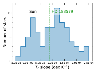
Figure 10: Histogram of abundance–condensation temperature ($T_{c}$) trends observed in a 79-star sample of solar twins studied by Bedell et al. (2018). HD 183579 is a member of this sample and its abundance pattern appears typical among solar twins. The abundance patterns for both HD 183579 and the general solar twin sample have been corrected for galactic chemical evolution effects as described in Bedell et al. (2018).

While the exact cause of the Sun’s atypical abundance pattern is still unclear, it is informative to look at HD 183579 as an example of a solar twin with a markedly different planetary system to the Sun’s. Many of the HARPS spectra used in this analysis were previously used to analyze the spectroscopic properties and abundances of HD 183579 at high precision using a line-by-line differential equivalent width technique (Spina et al., 2018; Bedell et al., 2018). The abundances of 30 elements were used to examine the behavior of abundance with $T_{c}$ for 79 solar twins, including HD 183579, in Bedell et al. (2018). Using the galactic chemical evolution-corrected abundance-$T_{c}$ relations measured in that work, we show that HD 183579 is a typical Sun-like star, without a statistically significant refractory element depletion (Figure 10).

All of these motivate us to examine if the majority of solar analogs hosting rocky planets (or planets with rocky cores, such as mini-Neptunes) show similar depletion as our Sun, or significant depletion. We used the homogeneous California-Kepler Survey (CKS) catalog to build our planet sample (Petigura et al., 2017; Johnson et al., 2017). There are a total of 1305 CKS spectra of “Kepler Objects of Interest” (KOIs) that hosting 2025 planet candidates, which precisely measure the stellar properties. We retrieved the publicly available abundances derived by Brewer et al. (2016) and Brewer & Fischer (2018), which achieved a typical internal abundance precision at $\sim 0.04$ dex level. We first threw out targets flagged as false positives or without dispositions in the catalog, leaving the stars with at least one or more confirmed planets/planet candidates. We then included stars with: (1) $\rm 5680\ K<T_{\rm eff}<5880\ K$; (2) $\rm\sigma_{T_{\rm eff}}<70\ K$; (3) $4.3\ {\rm dex}<\log g<4.5\ {\rm dex}$; (4) $\sigma_{\log g}<0.1\ {\rm dex}$; (5) $-0.1\ {\rm dex}<{\rm[Fe/H]}<0.1\ {\rm dex}$; (6) $\rm\sigma_{[Fe/H]}<0.05\ {\rm dex}$. We found 39 planet-host solar analogs. Since CKS only has a few known giant planet hosts and those systems may bias our comparison as the giant planet formation is also suspected to result in the depletion phenomenon (Booth & Owen, 2020), we further removed 3 systems with at least one planet with radius larger than 8$R_{\oplus}$ (KOI 1, KOI 372 and KOI 1089), thus our final sample contains 36 stars. We computed the mean abundance of each element (Na, Mg, Al, Si, Ca, Ti, Cr, Mn, Ni), and performed a least-square fit to the $\rm[X/Fe]$ as a function of the condensation temperature $T_{c}$. The result is presented in Figure 11. We tentatively found that solar analogs with rocky planets/rocky cores (i.e., mini-Neptunes) do not show a similar depletion as our Sun. However, this preliminary result is limited by the methodology used to derive the chemical abundance. With the current small number of precisely characterized solar twins with known planets, we cannot draw any conclusions.

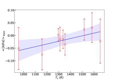
Figure 11: The mean abundance of the 36 CKS solar twin planet sample. The error bars represent the standard deviations of each elemental abundance. The blue solid line is the linear fit to the $T_{c}$ trend. The shaded region represents the $1\sigma$ confidence interval.

6 Discussion

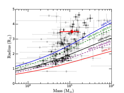
Figure 12: The mass radius diagram in Earth units. HD 183579b is marked as a red square. The confirmed planets with well measured radius and mass are shown as black points (uncertainty smaller than 20 %) while grey points represent the planet with poor constraint (data are retrieved from NASA Exoplanet Archive; Akeson et al. 2013). The colored lines are the theoretical M-R models for different planetary compositions, taken from Zeng & Sasselov (2013).

6.1 Atmospheric characterization of HD 183579b

Although thousands of large sub-Neptunes ($2.75\ R_{\oplus}<R_{p}<4\ R_{\oplus}$) have been detected up to now, only $\sim 40$ of them are orbiting around bright stars ($K<10$ mag). With $K=7.15$ mag, HD 183579b is hosted by the fifth brightest star among them (HD 21749b, Trifonov et al. 2019; Dragomir et al. 2019; Gan et al. 2021; GJ 436b, Butler et al. 2004; Knutson et al. 2011; HD 95338b, Díaz et al. 2020; and HD 3167c, Vanderburg et al. 2016; Livingston et al. 2018), making it an excellent target for future atmospheric characterization using the upcoming James Webb Space Telescope (JWST, Gardner et al. 2006) and Extremely Large Telescope (ELT, Gilmozzi & Spyromilio 2007; de Zeeuw et al. 2014).

Following the approach in Gillon et al. (2016), we estimated the signal amplitude of HD 183579b in the transit transmission spectroscopy:

$${\rm Amp}=\frac{2R_{p}h_{\rm eff}}{R_{\ast}^{2}},$$ (9)

where $R_{p}$ and $R_{\ast}$ are the planet and stellar radius, and $h_{\rm eff}=7kT/\mu g$ represents the effective atmospheric height. We adopted the typical atmospheric mean molecular mass $\mu$ to be 2.3 amu for sub-Neptune planets (Demory et al., 2020). Assuming the atmospheric temperature $T$ to be the equilibrium temperature $T_{\rm eq}$, we obtained an amplitude of $243^{+164}_{-75}$ ppm of HD 183579b, which is above the noise floor level 50 ppm of JWST for MIRI LRS ($\lambda=5.0-11\mu{\rm m}$) observations (Greene et al., 2016).

We further computed the Transmission Spectroscopy Metric (TSM; Kempton et al. 2018) of HD 183579b to be $126^{+168}_{-54}$. Kempton et al. (2018) recommended that planets with TSM$>90$ and $1.5<R_{p}<10\ R_{\oplus}$ are high-quality atmospheric characterization targets. Combined with the two aspects above, we regarded HD 183579b as an attractive source for further atmosphere composition analysis.

6.2 Prospects on Future Follow-up Observations

Since the current RV datasets only enable a $\sim 2\sigma$ mass constraint, here we suggest that future RVs measurements of HD 183579 are needed to break the degeneracy between the planet mass $M_{p}$ and the mean molecular weight $\mu$ (Seager & Sasselov, 2000; Seager et al., 2009) in any atmospheric characterization studies. Additional RVs would also be crucial to search for outer long period non-transiting cold giants (See the next subsection).

Given the brightness of HD 183579 ($V=8.7$ mag), most high resolution optical spectroscopy facilities like the Planet Finder Spectrograph (PFS; Crane et al. 2006; Crane et al. 2008, 2010) can achieve high SNR and reach the 1 m/s precision. In addition, the expected rotation timescale of HD 183579 is well separated from the planet orbital period, making it possible to smooth out the stellar activity effects in RVs with high cadence observations (López-Morales et al., 2016; Gan et al., 2021).

6.3 Additional planet in the HD 183579 system?

Zhu & Wu (2018) suggested a higher probability of detecting cold Jupiters around the hosts of small planets (planets with mass/radius between Earth and Neptune) compared with other field stars, which is also supported by the recent observational results from Bryan et al. (2019). As we have a long time baseline of HARPS observations ($\sim 3000$ d), we first looked for possible periodic signals on the residuals after subtracting the best-fit model for HD 183579b using GLS. However, we did not identify any significant peaks between 100 d and 1500 d with FAP<0.1%. We then ran another BM+1pl fit to blindly search the potential cold giant planets with period between the aforementioned range. We fit the Keplerian signals of HD 183579b and another potential outer cold planet simultaneously. By adopting the same prior settings for other parameters as the BM+1pl model in Section 4.2, we obtained $\Delta\ln Z=\ln Z_{\rm BM+1pl}-\ln Z_{\rm BM}=3$, which ruled out the existence of an outer gas giant planet with mass down to Saturn mass and period up to roughly 4 years based on the current data.

6.4 Comparison with Palatnick et al. 2021

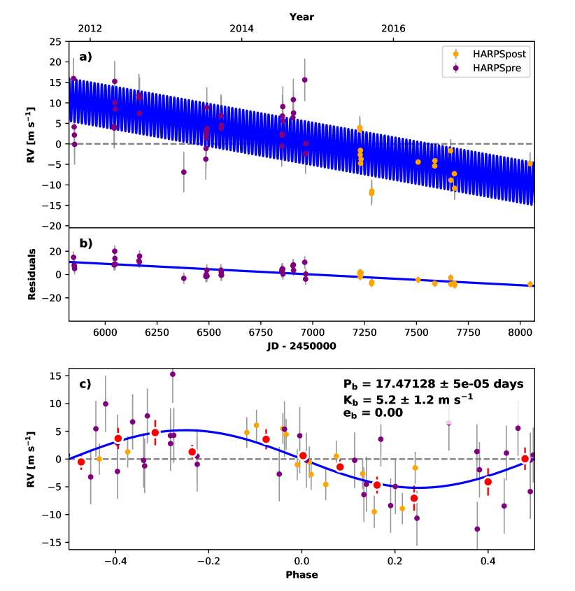
Figure 14: HARPS archive-only data used in Palatnick et al. (2021) and the best-fit model. The top panel shows the full RV time series and residuals. The phase-folded RV data are presented in the bottom panel. The red points are the binned RVs.

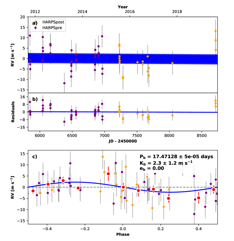
Figure 15: HARPS archive-only data plus three additional RV points along with the best-fit model. The top panel shows the full RV time series and residuals. The phase-folded RV data are presented in the bottom panel. The red points are the binned RVs. After including the new HARPS data, the model prefers a null RV slope (see Section 6.4).

We note that during the writing of this manuscript, Palatnick et al. (2021) validated this system using TESS and HARPS archival-only data (56 in total). The RV semi-amplitude of HD 183579 reported by Palatnick et al. (2021) is $4.9^{+0.9}_{-1.0}$ m/s, which is about $1.7\sigma$ larger than our measurement $2.7^{+1.3}_{-1.3}$ m/s. The discrepancy is caused by the contribution from the three recent, additional HARPS RV points taken between 2019 Aug. 16th and 2019 Aug. 20th in this work. All of the three newly acquired HARPS spectra have high SNR (105.9, 110.3 and 95.6, respectively). Without including these HARPS RV data, as in Palatnick et al. (2021), we derived a similar RV semi-amplitude of $K_{b}=5.2^{+1.1}_{-1.2}$ m/s by fitting a Keplerian model plus a linear RV slope $\dot{\gamma}$ using the same prior settings described in Section 4.2. The best-fit $\dot{\gamma}$ is $\rm-3.3^{+0.9}_{-0.9}\ m\ s^{-1}yr^{-1}$, consistent with the posterior value of $\rm-3.2^{+0.8}_{-0.7}\ m\ s^{-1}yr^{-1}$ reported in Palatnick et al. (2021). However, after including the three recent HARPS RV points, we found the model prefers a null RV slope ($\dot{\gamma}=-0.1^{+0.6}_{-0.8}\ {\rm m\ s^{-1}yr^{-1}}$) and the RV semi-amplitude decreases to $K_{b}=2.3^{+1.2}_{-1.2}$ m/s. We show both models in Figures 14 and 15. This difference is reasonable since the stellar activity plays a role in the Doppler signals, as stated in Section 3.2, which biases the result of Palatnick et al. (2021). Thus a Keplerian+RV slope model may not be able to explain the total HARPS data set. We emphasize here that our results are still consistent within $1.7\sigma$, and more RV data are needed to deal with the stellar activity and measure the mass of the planet more accurately.

7 Summary and Conclusions

In this paper, we characterize the HD 183579 planetary system using both space and ground-based photometric data from TESS and LCO as well as the spectroscopic data from HARPS and Minerva-Australis. Our models reveal that HD 183579b is a warm sub-Neptune hosted by a nearby solar twin with an orbital period of $17.47$ d, a radius of $3.53_{-0.11}^{+0.13}\ R_{\oplus}$ and a mass of $11.2_{-5.4}^{+5.4}\ M_{\oplus}$, with a $3\sigma$ upper limit of $27.4\ M_{\oplus}$ (see Figure 12). Taken together, the resulting planetary bulk density of $\rm 1.4^{+0.9}_{-0.8}\ g\ cm^{-3}$, implies that an extended atmosphere is likely present, making this system an excellent candidate for transmission spectroscopic follow-up. The line-by-line differential spectroscopic analysis shows that HD 183579 does not show a similar depletion in the abundance of refractory elements as our Sun. The lack of a Solar refractory depletion could plausibly be linked to HD 183579’s lack of known giant planets (following the gap-opening hypothesis) or a history of planetary migration and stellar infall, especially if the planet reported here did not form in-situ (following the planet accretion hypothesis).

Affiliations

¹Department of Astronomy and Tsinghua Centre for Astrophysics, Tsinghua University, Beijing 100084, China
²Center for Computational Astrophysics, Flatiron Institute, 162 Fifth Ave, New York, NY 10010, USA
³Departamento de Astronomia, IAG, Universidade de São Paulo, Rua do Matão 1226, São Paulo, 05509-900, Brazil
⁴National Astronomical Observatories, Chinese Academy of Sciences, 20A Datun Road, Chaoyang District, Beijing 100012, China
⁵Department of Physics and Astronomy, Vanderbilt University, 6301 Stevenson Center Ln., Nashville, TN 37235, USA
⁶Department of Physics, Fisk University, 1000 17th Avenue North, Nashville, TN 37208, USA
⁷NASA Ames Research Center, Moffett Field, CA 94035, USA
⁸Department of Physics, Engineering and Astronomy, Stephen F. Austin State University, 1936 North St, Nacogdoches, TX 75962, USA
⁹University of Southern Queensland, Centre for Astrophysics, West Street, Toowoomba, QLD 4350 Australia
¹⁰Astrophysics Group, Keele University, Staffordshire, ST5 5BG, UK
¹¹Center for Astrophysics ${\rm\mid}$ Harvard & Smithsonian, 60 Garden Street, Cambridge, MA 02138, USA
¹²Department of Physics and Kavli Institute for Astrophysics and Space Research, Massachusetts Institute of Technology, Cambridge, MA 02139, USA
¹³Department of Earth, Atmospheric and Planetary Sciences, Massachusetts Institute of Technology, Cambridge, MA 02139, USA
¹⁴Department of Aeronautics and Astronautics, MIT, 77 Massachusetts Avenue, Cambridge, MA 02139, USA
¹⁵Department of Astrophysical Sciences, Princeton University, 4 Ivy Lane, Princeton, NJ 08544, USA
¹⁶Department of Astronomy, University of Florida, 211 Bryant Space Science Center, Gainesville, FL, 32611, USA
¹⁷NASA Goddard Space Flight Center, 8800 Greenbelt Road, Greenbelt, MD 20771, USA
¹⁸University of Maryland, Baltimore County, 1000 Hilltop Circle, Baltimore, MD 21250, USA
¹⁹Department of Astronomy and Astrophysics, University of Chicago, 5640 S. Ellis Ave, Chicago, IL 60637, USA
²⁰Department of Astronomy, The University of Texas at Austin, TX 78712, USA
²¹Cerro Tololo Inter-American Observatory, Casilla 603, La Serena, Chile
²²Department of Physics & Astronomy, University of Kansas, 1082 Malott,1251 Wescoe Hall Dr., Lawrence, KS 66045, USA
²³Max Planck Institute for Astronomy, Konigstuhl 17, 69117 Heidelberg, Germany
²⁴Department of Physics & Astronomy, Swarthmore College, Swarthmore PA 19081, USA
²⁵Department of Earth and Planetary Sciences, University of California, Riverside, CA 92521, USA
²⁶Department of Physics and Astronomy, University of Louisville, Louisville, KY 40292, USA
²⁷Department of Physics and Astronomy, The University of North Carolina at Chapel Hill, Chapel Hill, NC 27599-3255, USA
²⁸NCCR/PlanetS, Centre for Space & Habitability, University of Bern, Bern, Switzerland
²⁹George Mason University, 4400 University Drive MS 3F3, Fairfax, VA 22030, USA
³⁰Patashnick Voorheesville Observatory, Voorheesville, NY 12186, USA
³¹Space Telescope Science Institute, 3700 San Martin Drive, Baltimore, MD 21218, USA
³²SETI Institute, 189 Bernardo Ave, Suite 200, Mountain View, CA 94043, USA
³³INAF - Osservatorio Astronomico di Padova, vicolo dell’Osservatorio 5, 35122, Padova, Italy
³⁴Exoplanetary Science at UNSW, School of Physics, UNSW Sydney, NSW 2052, Australia
³⁵Tsinghua International School, Beijing 100084, China
³⁶Stanford Online High School, 415 Broadway Academy Hall, Floor 2, 8853, Redwood City, CA 94063, USA
³⁷School of Astronomy and Space Science, Key Laboratory of Modern Astronomy and Astrophysics in Ministry of Education, Nanjing University, Nanjing 210046, Jiangsu, China

Data Availability

This paper includes photometric data collected by the TESS mission and LCOGT, which is publicly available in ExoFOP, at https://exofop.ipac.caltech.edu/tess/target.php?id=320004517. All spectroscopy data underlying this article are listed in the appendix.

Appendix A All RVs and stellar activity indicators of HARPS and Minerva-Australis

Table 5: HARPS RVs and stellar activity indicators

Time (BJD)	RV (m/s)	RVerr (m/s)	CRX	CRXerr	DLW	DLWerr	BIS	FWHM	$S_{\rm HK}$	$S_{\rm HK}$err
2455847.536	14.37	1.53	-1.16	12.18	1.99	2.49	-0.025	7.091	0.1821	0.0014
2455850.515	2.02	0.82	-10.75	6.45	-1.97	1.27	-0.016	7.079	0.191	0.0008
2455851.518	-0.3	0.71	1.63	5.75	-7.83	1.18	-0.015	7.068	0.1901	0.0007
2455852.505	-1.39	1.22	3.17	9.84	-10.34	1.64	-0.019	7.062	0.1897	0.0009
2456042.793	4.35	1.15	11.92	9.15	-10.75	1.47	-0.024	7.073	0.1852	0.001
2456043.878	3.59	1.21	-3.85	9.74	-8.64	1.55	-0.019	7.074	0.1854	0.001
2456045.888	15.57	1.37	-25.38	10.55	-2.59	2.25	-0.018	7.078	0.1894	0.0012
2456046.939	10.58	0.86	-17.16	6.6	7.91	1.27	-0.017	7.082	0.1909	0.0009
2456048.942	7.96	0.97	-8.24	7.75	19.62	1.82	-0.015	7.075	0.1944	0.0009
2456162.592	10.61	2.11	-14.78	16.61	6.19	3.48	-0.014	7.087	0.1872	0.0018
2456164.651	7.01	1.49	-10.12	11.79	-2.52	2.14	-0.017	7.082	0.1972	0.0015
2456165.633	9.13	1.01	-8.8	8.1	-1.67	1.44	-0.019	7.072	0.1965	0.0009
2456378.907	-7.67	0.82	14.47	6.39	-0.23	1.1	-0.019	7.073	0.1892	0.0008
2456484.744	-3.47	1.81	35.43	13.85	-0.01	2.17	-0.026	7.09	0.1769	0.0014
2456485.724	-2.08	1.03	19.75	7.82	-3.14	1.34	-0.021	7.081	0.1912	0.0008
2456486.702	1.27	0.93	23.83	6.83	0.36	0.89	-0.024	7.084	0.1945	0.0007
2456487.706	2.01	0.96	27.73	6.86	-0.97	0.93	-0.022	7.081	0.195	0.0007
2456488.727	3.66	0.98	29.05	6.91	2.78	1.23	-0.022	7.087	0.1939	0.0009
2456489.694	7.93	0.99	-12.21	7.79	5.59	1.36	-0.011	7.09	0.1934	0.0009
2456490.7	1.49	0.92	-16.04	7.1	2.04	1.19	-0.018	7.081	0.1928	0.0008
2456557.59	6.92	1.65	12.62	12.95	4.51	3.16	-0.017	7.087	0.1926	0.0018
2456558.572	3.15	0.98	2.53	7.89	-0.06	1.18	-0.02	7.073	0.191	0.0008
2456559.583	7.07	1.06	-11.08	8.36	-2.82	1.43	-0.02	7.077	0.1885	0.001
2456560.578	3.09	0.83	-13.03	6.48	0.53	1.15	-0.023	7.071	0.189	0.0008
2456850.714	-0.38	1.23	-6.28	9.74	6.38	1.74	-0.017	7.072	0.1932	0.0012
2456851.725	2.3	1.04	-7.54	8.29	5.97	1.36	-0.016	7.076	0.1869	0.001
2456852.73	1.74	1.07	-19.51	8.19	-1.3	1.71	-0.021	7.075	0.1939	0.001
2456853.794	9.94	1.93	-6.63	15.39	5.63	2.25	-0.018	7.088	0.173	0.0014
2456855.725	8.36	1.11	-17.74	8.68	1.32	1.45	-0.02	7.083	0.1916	0.0009
2456856.715	4.03	0.83	-13.81	6.47	3.66	1.27	-0.015	7.084	0.1947	0.0009
2456904.574	5.07	0.92	-21.63	6.78	-1.63	1.28	-0.023	7.074	0.1872	0.0009
2456906.573	5.58	1.58	6.81	12.49	1.74	2.79	-0.018	7.079	0.1792	0.0015
2456907.587	4.38	1.24	-13.04	9.71	1.04	1.76	-0.022	7.076	0.194	0.0012
2456961.505	11.57	2.43	-7.7	19.4	5.59	3.13	-0.028	7.083	0.1818	0.0019
2456965.501	-3.57	0.75	1.78	6.02	-0.66	0.97	-0.021	7.082	0.1885	0.0007
2456966.521	-1.39	1.01	0.58	8.2	-2.71	1.35	-0.023	7.079	0.1893	0.0009
2457226.716	10.4	0.96	-3.69	7.98	4.29	1.1	-0.004	7.1	0.1934	0.0007
2457227.703	10.21	1.11	-4.51	9.22	4.28	0.9	-0.007	7.104	0.1953	0.0007
2457228.698	4.03	1.22	-6.97	10.15	4.88	1.3	-0.004	7.104	0.196	0.001
2457229.711	4.87	1.07	0.36	9.06	4.28	0.79	-0.004	7.1	0.1927	0.0006
2457230.698	1.2	0.92	1.46	7.79	2.64	0.83	-0.004	7.095	0.1891	0.0006
2457232.67	1.54	1.52	-7.21	12.74	3.76	1.83	-0.002	7.104	0.1861	0.0012
2457283.549	-6.69	1.56	0.72	12.94	-5.74	2.0	-0.004	7.088	0.1875	0.0011
2457284.601	-5.29	1.05	7.82	8.72	-2.45	1.1	-0.009	7.09	0.1889	0.0008
2457507.88	2.41	1.5	-1.29	12.65	7.57	1.16	-0.004	7.117	0.1824	0.0006
2457587.718	1.44	1.06	4.99	8.79	-4.88	1.24	-0.007	7.087	0.1807	0.0008
2457588.767	1.86	1.02	-9.51	8.38	-5.32	0.91	0.036	7.139	0.1791	0.0008
2457588.78	2.33	1.08	0.07	8.89	-4.64	1.46	-0.012	7.082	0.1797	0.0009
2457664.611	3.37	0.96	-9.33	7.8	-5.5	0.97	-0.005	7.095	0.1857	0.0008
2457665.549	-2.78	1.04	9.86	8.57	-3.84	1.14	-0.006	7.096	0.184	0.0008
2457682.499	-1.45	0.85	9.3	6.97	-3.19	1.08	-0.013	7.09	0.186	0.0007
2457683.568	-3.81	0.97	3.03	8.04	-7.46	1.26	-0.018	7.088	0.1875	0.001
2458047.504	0.16	0.98	-2.6	8.15	-3.8	0.67	-0.009	7.088	0.184	0.0006
2458711.619	15.76	1.18	4.2	9.88	2.83	1.19	-0.008	7.1	0.204	0.0008
2458713.76	13.1	1.14	9.7	9.52	5.74	1.38	-0.006	7.102	0.1998	0.001
2458715.714	8.67	1.08	-10.43	9.04	2.9	1.14	-0.009	7.103	0.2021	0.0009

Table 6: Minerva-Australis RVs of 4 telescopes: MA, MB, MC and MD

Time(BJD)	RV(m/s)	RVerr(m/s)	Instrument
2458961.205	13.51	8.03	MA
2458964.276	-5.64	8.17	MA
2458966.254	0.3	8.35	MA
2458980.084	-6.58	8.67	MA
2458981.194	20.78	7.4	MA
2458959.285	-17.62	5.0	MB
2458961.205	11.8	6.36	MB
2458964.276	-4.74	5.22	MB
2458966.254	-1.2	5.29	MB
2458971.214	1.2	8.62	MB
2458971.236	-17.36	8.93	MB
2458973.184	19.1	5.2	MB
2458973.206	13.31	5.17	MB
2458959.285	-34.61	6.39	MC
2458961.205	-14.81	7.23	MC
2458964.276	-28.45	6.54	MC
2458966.254	-41.26	6.91	MC
2458973.184	8.17	6.09	MC
2458973.206	9.67	6.35	MC
2458974.308	1.66	7.46	MC
2458980.084	-0.27	8.1	MC
2458980.106	20.03	8.04	MC
2458981.172	7.12	6.76	MC
2458981.194	14.62	6.66	MC
2458995.32	-31.32	8.98	MC
2458998.047	-11.82	6.91	MC
2458998.069	9.99	6.86	MC
2459002.078	-13.7	7.22	MC
2458995.32	-20.95	5.55	MD
2458998.047	6.44	6.23	MD
2458998.069	0.0	5.57	MD
2459002.078	-3.96	5.75	MD
2459002.099	3.82	7.18	MD

Appendix B BM for HARPS and Minerva

Appendix C Model Comparison

References

- Addison et al. (2019) Addison B., et al., 2019, PASP, 131, 115003
- Addison et al. (2020) Addison B. C., et al., 2020, arXiv e-prints, p. arXiv:2006.13675
- Addison et al. (2021) Addison B. C., et al., 2021, MNRAS, 502, 3704
- Adibekyan et al. (2014) Adibekyan V. Z., González Hernández J. I., Delgado Mena E., Sousa S. G., Santos N. C., Israelian G., Figueira P., Bertran de Lis S., 2014, A&A, 564, L15
- Akeson et al. (2013) Akeson R. L., et al., 2013, PASP, 125, 989
- Aller et al. (2020) Aller A., Lillo-Box J., Jones D., Miranda L. F., Barceló Forteza S., 2020, A&A, 635, A128
- Angus et al. (2016) Angus R., Foreman-Mackey D., Johnson J. A., 2016, ApJ, 818, 109
- Astropy Collaboration et al. (2013) Astropy Collaboration et al., 2013, A&A, 558, A33
- Astropy Collaboration et al. (2018) Astropy Collaboration et al., 2018, AJ, 156, 123
- Baglin et al. (2006) Baglin A., Auvergne M., Barge P., Deleuil M., Catala C., Michel E., Weiss W., COROT Team 2006, in Fridlund M., Baglin A., Lochard J., Conroy L., eds, ESA Special Publication Vol. 1306, The CoRoT Mission Pre-Launch Status - Stellar Seismology and Planet Finding. p. 33
- Bakos et al. (2004) Bakos G., Noyes R. W., Kovács G., Stanek K. Z., Sasselov D. D., Domsa I., 2004, PASP, 116, 266
- Barentsen et al. (2019) Barentsen G., et al., 2019, KeplerGO/lightkurve: Lightkurve v1.0b29, doi:10.5281/zenodo.2565212, https://doi.org/10.5281/zenodo.2565212
- Barnes (2007) Barnes S. A., 2007, ApJ, 669, 1167
- Barnes et al. (2012) Barnes S. I., Gibson S., Nield K., Cochrane D., 2012, in Ground-based and Airborne Instrumentation for Astronomy IV. p. 844688, doi:10.1117/12.926527
- Bedell et al. (2015) Bedell M., et al., 2015, A&A, 581, A34
- Bedell et al. (2018) Bedell M., et al., 2018, ApJ, 865, 68
- Bensby et al. (2003) Bensby T., Feltzing S., Lundström I., 2003, A&A, 410, 527
- Bensby et al. (2014) Bensby T., Feltzing S., Oey M. S., 2014, A&A, 562, A71
- Booth & Owen (2020) Booth R. A., Owen J. E., 2020, MNRAS, 493, 5079
- Borucki et al. (2010) Borucki W. J., et al., 2010, Science, 327, 977
- Bovy (2015) Bovy J., 2015, ApJS, 216, 29
- Brewer & Fischer (2018) Brewer J. M., Fischer D. A., 2018, ApJS, 237, 38
- Brewer et al. (2016) Brewer J. M., Fischer D. A., Valenti J. A., Piskunov N., 2016, ApJS, 225, 32
- Brown (2003) Brown T. M., 2003, ApJ, 593, L125
- Brown et al. (2013) Brown T. M., et al., 2013, PASP, 125, 1031
- Bryan et al. (2019) Bryan M. L., Knutson H. A., Lee E. J., Fulton B. J., Batygin K., Ngo H., Meshkat T., 2019, AJ, 157, 52
- Butler et al. (2004) Butler R. P., Vogt S. S., Marcy G. W., Fischer D. A., Wright J. T., Henry G. W., Laughlin G., Lissauer J. J., 2004, ApJ, 617, 580
- Chambers (2010) Chambers J. E., 2010, ApJ, 724, 92
- Chazelas et al. (2012) Chazelas B., et al., 2012, in Ground-based and Airborne Telescopes IV. p. 84440E, doi:10.1117/12.925755
- Chen & Kipping (2017) Chen J., Kipping D., 2017, ApJ, 834, 17
- Church et al. (2020) Church R. P., Mustill A. J., Liu F., 2020, MNRAS, 491, 2391
- Clark et al. (2021) Clark J. T., et al., 2021, MNRAS, 504, 4968
- Collins et al. (2017) Collins K. A., Kielkopf J. F., Stassun K. G., Hessman F. V., 2017, AJ, 153, 77
- Crane et al. (2006) Crane J. D., Shectman S. A., Butler R. P., 2006, The Carnegie Planet Finder Spectrograph. p. 626931, doi:10.1117/12.672339
- Crane et al. (2008) Crane J. D., Shectman S. A., Butler R. P., Thompson I. B., Burley G. S., 2008, The Carnegie Planet Finder Spectrograph: a status report. p. 701479, doi:10.1117/12.789637
- Crane et al. (2010) Crane J. D., Shectman S. A., Butler R. P., Thompson I. B., Birk C., Jones P., Burley G. S., 2010, The Carnegie Planet Finder Spectrograph: integration and commissioning. p. 773553, doi:10.1117/12.857792
- Curtis et al. (2018) Curtis J. L., et al., 2018, AJ, 155, 173
- Curtis et al. (2019) Curtis J. L., Agüeros M. A., Douglas S. T., Meibom S., 2019, ApJ, 879, 49
- Cutri et al. (2003) Cutri R. M., et al., 2003, 2MASS All Sky Catalog of point sources.
- Demory et al. (2020) Demory B. O., et al., 2020, A&A, 642, A49
- Díaz et al. (2020) Díaz M. R., et al., 2020, MNRAS, 496, 4330
- Dragomir et al. (2019) Dragomir D., et al., 2019, ApJ, 875, L7
- Espinoza (2018) Espinoza N., 2018, Research Notes of the American Astronomical Society, 2, 209
- Espinoza et al. (2019) Espinoza N., Kossakowski D., Brahm R., 2019, MNRAS, 490, 2262
- Feng et al. (2017) Feng F., Tuomi M., Jones H. R. A., 2017, MNRAS, 470, 4794
- Foreman-Mackey et al. (2017) Foreman-Mackey D., Agol E., Ambikasaran S., Angus R., 2017, AJ, 154, 220
- Foreman-Mackey et al. (2020) Foreman-Mackey D., Luger R., Czekala I., Agol E., Price-Whelan A., Barclay T., 2020, exoplanet-dev/exoplanet v0.3.2, doi:10.5281/zenodo.1998447, https://doi.org/10.5281/zenodo.1998447
- Fulton et al. (2018) Fulton B. J., Petigura E. A., Blunt S., Sinukoff E., 2018, PASP, 130, 044504
- Gaia Collaboration et al. (2018) Gaia Collaboration et al., 2018, A&A, 616, A1
- Gaia Collaboration et al. (2021) Gaia Collaboration et al., 2021, A&A, 649, A1
- Gan et al. (2020) Gan T., et al., 2020, AJ, 159, 160
- Gan et al. (2021) Gan T., et al., 2021, MNRAS, 501, 6042
- Gardner et al. (2006) Gardner J. P., et al., 2006, Space Sci. Rev., 123, 485
- Gillon et al. (2016) Gillon M., et al., 2016, Nature, 533, 221
- Gilmozzi & Spyromilio (2007) Gilmozzi R., Spyromilio J., 2007, The Messenger, 127
- Greene et al. (2016) Greene T. P., Line M. R., Montero C., Fortney J. J., Lustig-Yaeger J., Luther K., 2016, ApJ, 817, 17
- Higson et al. (2019) Higson E., Handley W., Hobson M., Lasenby A., 2019, Statistics and Computing, 29, 891
- Hinkel & Unterborn (2018) Hinkel N. R., Unterborn C. T., 2018, ApJ, 853, 83
- Hirano et al. (2018) Hirano T., et al., 2018, AJ, 155, 124
- Høg et al. (2000) Høg E., et al., 2000, A&A, 355, L27
- Horner et al. (2020) Horner J., et al., 2020, PASP, 132, 102001
- Howell et al. (2011) Howell S. B., Everett M. E., Sherry W., Horch E., Ciardi D. R., 2011, AJ, 142, 19
- Howell et al. (2014) Howell S. B., et al., 2014, PASP, 126, 398
- Huang et al. (2018) Huang C. X., et al., 2018, preprint, (arXiv:1807.11129)
- Husser et al. (2013) Husser T.-O., Wende-von Berg S., Dreizler S., Homeier D., Reiners A., Barman T., Hauschildt P. H., 2013, A&A, 553, A6
- Jenkins (2002) Jenkins J. M., 2002, ApJ, 575, 493
- Jenkins et al. (2016) Jenkins J. M., et al., 2016, in Software and Cyberinfrastructure for Astronomy IV. p. 99133E, doi:10.1117/12.2233418
- Jenkins et al. (2017) Jenkins J. M., Tenenbaum P., Seader S., Burke C. J., McCauliff S. D., Smith J. C., Twicken J. D., Chandrasekaran H., 2017, Technical report, Kepler Data Processing Handbook: Transiting Planet Search
- Jensen (2013) Jensen E., 2013, Tapir: A web interface for transit/eclipse observability (ascl:1306.007)
- Johnson & Soderblom (1987) Johnson D. R. H., Soderblom D. R., 1987, AJ, 93, 864
- Johnson et al. (2017) Johnson J. A., et al., 2017, AJ, 154, 108
- Jordán et al. (2020) Jordán A., et al., 2020, AJ, 159, 145
- Kane et al. (2021) Kane S. R., et al., 2021, Journal of Geophysical Research (Planets), 126, e06643
- Kempton et al. (2018) Kempton E. M. R., et al., 2018, PASP, 130, 114401
- Kipping (2013) Kipping D. M., 2013, MNRAS, 435, 2152
- Knutson et al. (2011) Knutson H. A., et al., 2011, ApJ, 735, 27
- Kovács et al. (2002) Kovács G., Zucker S., Mazeh T., 2002, A&A, 391, 369
- Kreidberg (2015) Kreidberg L., 2015, PASP, 127, 1161
- Labadie-Bartz et al. (2019) Labadie-Bartz J., et al., 2019, ApJS, 240, 13
- Li et al. (2019) Li J., Tenenbaum P., Twicken J. D., Burke C. J., Jenkins J. M., Quintana E. V., Rowe J. F., Seader S. E., 2019, PASP, 131, 024506
- Lightkurve Collaboration et al. (2018) Lightkurve Collaboration et al., 2018, Lightkurve: Kepler and TESS time series analysis in Python (ascl:1812.013)
- Lissauer et al. (2011) Lissauer J. J., et al., 2011, Nature, 470, 53
- Livingston et al. (2018) Livingston J. H., et al., 2018, AJ, 156, 277
- Lo Curto et al. (2015) Lo Curto G., et al., 2015, The Messenger, 162, 9
- Lodders (2003) Lodders K., 2003, ApJ, 591, 1220
- Lomb (1976) Lomb N. R., 1976, Ap&SS, 39, 447
- López-Morales et al. (2016) López-Morales M., et al., 2016, AJ, 152, 204
- Lorenzo-Oliveira et al. (2018) Lorenzo-Oliveira D., et al., 2018, A&A, 619, A73
- Lovis et al. (2011) Lovis C., et al., 2011, arXiv e-prints, p. arXiv:1107.5325
- Mamajek & Hillenbrand (2008) Mamajek E. E., Hillenbrand L. A., 2008, ApJ, 687, 1264
- Mayor & Queloz (1995) Mayor M., Queloz D., 1995, Nature, 378, 355
- Mayor et al. (2003) Mayor M., et al., 2003, The Messenger, 114, 20
- McCully et al. (2018) McCully C., Volgenau N. H., Harbeck D.-R., Lister T. A., Saunders E. S., Turner M. L., Siiverd R. J., Bowman M., 2018, in Software and Cyberinfrastructure for Astronomy V. p. 107070K (arXiv:1811.04163), doi:10.1117/12.2314340
- McQuillan et al. (2014) McQuillan A., Mazeh T., Aigrain S., 2014, ApJS, 211, 24
- Meibom et al. (2009) Meibom S., Mathieu R. D., Stassun K. G., 2009, ApJ, 695, 679
- Meléndez et al. (2009) Meléndez J., Asplund M., Gustafsson B., Yong D., 2009, ApJ, 704, L66
- Meléndez et al. (2015) Meléndez J., et al., 2015, The Messenger, 161, 28
- Morrissey et al. (2007) Morrissey P., et al., 2007, ApJS, 173, 682
- Mortier et al. (2015) Mortier A., Faria J. P., Correia C. M., Santerne A., Santos N. C., 2015, A&A, 573, A101
- Nissen (2015) Nissen P. E., 2015, A&A, 579, A52
- Oh et al. (2018) Oh S., Price-Whelan A. M., Brewer J. M., Hogg D. W., Spergel D. N., Myles J., 2018, ApJ, 854, 138
- Olspert et al. (2018) Olspert N., Pelt J., Käpylä M. J., Lehtinen J., 2018, A&A, 615, A111
- Palatnick et al. (2021) Palatnick S., Kipping D., Yahalomi D., 2021, ApJ, 909, L6
- Parviainen & Aigrain (2015) Parviainen H., Aigrain S., 2015, MNRAS, 453, 3821
- Paunzen (2015) Paunzen E., 2015, A&A, 580, A23
- Pepe et al. (2002) Pepe F., Mayor M., Galland F., Naef D., Queloz D., Santos N. C., Udry S., Burnet M., 2002, A&A, 388, 632
- Pepper et al. (2007) Pepper J., et al., 2007, PASP, 119, 923
- Pepper et al. (2012) Pepper J., Kuhn R. B., Siverd R., James D., Stassun K., 2012, PASP, 124, 230
- Petigura et al. (2017) Petigura E. A., et al., 2017, AJ, 154, 107
- Pollacco et al. (2006) Pollacco D. L., et al., 2006, PASP, 118, 1407
- Ramírez et al. (2009) Ramírez I., Meléndez J., Asplund M., 2009, A&A, 508, L17
- Ramírez et al. (2011) Ramírez I., Meléndez J., Cornejo D., Roederer I. U., Fish J. R., 2011, ApJ, 740, 76
- Ramírez et al. (2014) Ramírez I., et al., 2014, A&A, 572, A48
- Ricker et al. (2014) Ricker G. R., et al., 2014, in Space Telescopes and Instrumentation 2014: Optical, Infrared, and Millimeter Wave. p. 914320 (arXiv:1406.0151), doi:10.1117/12.2063489
- Ricker et al. (2015) Ricker G. R., et al., 2015, Journal of Astronomical Telescopes, Instruments, and Systems, 1, 014003
- Salvatier et al. (2016) Salvatier J., Wiecki T. V., Fonnesbeck C., 2016, PeerJ Computer Science, 2, e55
- Scargle (1982) Scargle J. D., 1982, ApJ, 263, 835
- Schlegel et al. (1998) Schlegel D. J., Finkbeiner D. P., Davis M., 1998, ApJ, 500, 525
- Seager & Sasselov (2000) Seager S., Sasselov D. D., 2000, ApJ, 537, 916
- Seager et al. (2009) Seager S., Deming D., Valenti J. A., 2009, Astrophysics and Space Science Proceedings, 10, 123
- Skrutskie et al. (2006) Skrutskie M. F., et al., 2006, AJ, 131, 1163
- Smith et al. (2012) Smith J. C., et al., 2012, PASP, 124, 1000
- Soto & Jenkins (2018) Soto M. G., Jenkins J. S., 2018, A&A, 615, A76
- Speagle (2020) Speagle J. S., 2020, MNRAS,
- Spina et al. (2015) Spina L., et al., 2015, A&A, 582, L6
- Spina et al. (2016) Spina L., Meléndez J., Ramírez I., 2016, A&A, 585, A152
- Spina et al. (2018) Spina L., et al., 2018, MNRAS, 474, 2580
- Stassun & Torres (2016) Stassun K. G., Torres G., 2016, AJ, 152, 180
- Stassun et al. (2017) Stassun K. G., Collins K. A., Gaudi B. S., 2017, AJ, 153, 136
- Stassun et al. (2018a) Stassun K. G., Corsaro E., Pepper J. A., Gaudi B. S., 2018a, AJ, 155, 22
- Stassun et al. (2018b) Stassun K. G., et al., 2018b, AJ, 156, 102
- Stassun et al. (2019) Stassun K. G., et al., 2019, AJ, 158, 138
- Stumpe et al. (2012) Stumpe M. C., et al., 2012, PASP, 124, 985
- Stumpe et al. (2014) Stumpe M. C., Smith J. C., Catanzarite J. H., Van Cleve J. E., Jenkins J. M., Twicken J. D., Girouard F. R., 2014, PASP, 126, 100
- Sullivan et al. (2015) Sullivan P. W., et al., 2015, ApJ, 809, 77
- Theano Development Team (2016) Theano Development Team 2016, arXiv e-prints, abs/1605.02688
- Tokovinin (2018) Tokovinin A., 2018, PASP, 130, 035002
- Torres et al. (2010) Torres G., Andersen J., Giménez A., 2010, A&ARv, 18, 67
- Trifonov et al. (2019) Trifonov T., Rybizki J., Kürster M., 2019, A&A, 622, L7
- Trotta (2008) Trotta R., 2008, Contemporary Physics, 49, 71
- Twicken et al. (2018) Twicken J. D., et al., 2018, PASP, 130, 064502
- Vanderburg et al. (2016) Vanderburg A., et al., 2016, ApJ, 829, L9
- Wheatley et al. (2018) Wheatley P. J., et al., 2018, MNRAS, 475, 4476
- Wright & Eastman (2014) Wright J. T., Eastman J. D., 2014, PASP, 126, 838
- Wright et al. (2010) Wright E. L., et al., 2010, AJ, 140, 1868
- Yana Galarza et al. (2016) Yana Galarza J., Meléndez J., Ramírez I., Yong D., Karakas A. I., Asplund M., Liu F., 2016, A&A, 589, A17
- Yee et al. (2017) Yee S. W., Petigura E. A., von Braun K., 2017, ApJ, 836, 77
- Zechmeister et al. (2018) Zechmeister M., et al., 2018, A&A, 609, A12
- Zeng & Sasselov (2013) Zeng L., Sasselov D., 2013, PASP, 125, 227
- Zhu & Wu (2018) Zhu W., Wu Y., 2018, AJ, 156, 92
- Ziegler et al. (2020) Ziegler C., Tokovinin A., Briceño C., Mang J., Law N., Mann A. W., 2020, AJ, 159, 19
- de Zeeuw et al. (2014) de Zeeuw T., Tamai R., Liske J., 2014, The Messenger, 158, 3