Sparse Joint Transmission for Cloud Radio Access Networks with Limited Fronthaul Capacity

Abstract

A cloud radio access network (C-RAN) is a promising cellular network, wherein densely deployed multi-antenna remote-radio-heads (RRHs) jointly serve many users using the same time-frequency resource. By extremely high signaling overheads for both channel state information (CSI) acquisition and data sharing at a baseband unit (BBU), finding a joint transmission strategy with a significantly reduced signaling overhead is indispensable to achieve the cooperation gain in practical C-RANs. In this paper, we present a novel sparse joint transmission (sparse-JT) method for C-RANs, where the number of transmit antennas per unit area is much larger than the active downlink user density. Considering the effects of noisy-and-incomplete CSI and the quantization errors in data sharing by a finite-rate fronthaul capacity, the key innovation of sparse-JT is to find a joint solution for cooperative RRH clusters, beamforming vectors, and power allocation to maximize a lower bound of the sum-spectral efficiency under the sparsity constraint of active RRHs. To find such a solution, we present a computationally efficient algorithm that guarantees to find a local-optimal solution for a relaxed sum-spectral efficiency maximization problem. By system-level simulations, we exhibit that sparse-JT provides significant gains in ergodic spectral efficiencies compared to existing joint transmissions.

I Introduction

I-A Motivation

Next-generation cellular networks, including 6G, require to support demands on high speed and uniform data services [boccardi2014five]. The ever-growing demands for higher bit rates and more uniform data services necessitate novel cellular network architectures that can yield high network capacity within a limited spectrum. The new cellular architectures providing an increased network capacity are expected to have two key ingredients: 1) densely deployed base stations (BSs) topologies that aggressively reuse spectrum [ge20165g] and 2) the coordination among the BSs to eliminate both inter-user and inter-cell interference [gesbert2010multi, lozano2013fundamental, lee2014spectral].

A cloud radio access network (C-RAN) [chen2011c, boccardi2014five, gesbert2010multi, lozano2013fundamental, lee2014spectral] is a promising cellular architecture to achieve high energy and spectral efficiencies by both network densification and BS cooperation gains. A cloud-RAN consists of distributed antennas, called remote radio heads (RRHs), connected to a centralized baseband unit (BBU) pool via high-speed fronthaul links. This network virtually forms a large-scale distributed and cooperative MIMO system. The centralized BBU pool can jointly perform user selection, beamforming, and power allocation for both downlink and uplink communications to eliminate interference between scheduled users. As the network density increases, this joint processing allows to achieve a high cell-splitting gain by reducing the communication distance between the network and the mobile users; thereby, it can significantly dwindle the transmission power.

Unfortunately, in practice, the promising gain by the joint transmission comes at the cost of prohibitively high signaling overhead. Specifically, for downlink communications, BBU needs to acquire global channel state information (CSI) and to share the precoded data with RRHs. As the network becomes denser, the amount of signaling overheads for CSI acquisition and data sharing increases tremendously. Moreover, acquiring global CSI perfectly and sharing the precoded data without any error is impossible due to a finite-rate fronthaul capacity. For instance, in C-RAN operating with time-division-duplexing (TDD) mode, each RRH estimates users’ channels via uplink pilots and sends them to BBU via a finite-rate fronthaul link. Therefore, the accuracy of CSI at BBU is fundamentally limited by both channel estimation errors and the fronthaul capacity. Furthermore, the precoded data symbols at BBU are shared with RRHs through finite-rate fronthaul links for the downlink transmission. A low-rate fronthaul link introduces a high quantization error on the downlink data; this leads to the degradation of the downlink performance. Considering the signaling overheads and limited fronthaul capacity constraints, the effective gain of the joint processing offered by C-RANs can be very marginal.

To enhance the effective gain in practice, the joint transmission exploiting a few dynamically selected RRHs is a promising solution because it can considerably reduce the signaling overheads associated with the joint processing. For example, from the users’ viewpoint, it is better to receive the downlink signals from all RRHs to increase data rates. Whereas, from the network perspective, the use of all RRHs increases the associated signaling overheads for joint transmission. In particular, when the active user density is much smaller than the total number of antennas per unit area in the network, the use of sparsely chosen RRHs would be sufficient for joint transmission, while it considerably reduces the overheads. In this sense, it is essential to use a sparse RRH cooperation method to form a large-scale C-RAN. Unfortunately, finding the jointly optimal solution for the sparsely chosen cooperative RRH sets per user, precoding vectors, and transmit power, which maximizes the downlink sum-spectral efficiency, is a well-known NP-hard problem [luo2008dynamic, yu2013multicell, hong2013joint], even under assumptions of the perfect and global CSI and the infinite-rate fronthaul capacity. Considering the practical constraints of a finite-rate capacity of fronthaul links and noisy and partial CSI, finding a local-optimal solution for the sum-spectral efficiency maximization problem is highly non-trivial. To tackle this problem, this paper introduces a novel sparse joint downlink transmission technique that maximizes a lower bound of the sum-spectral efficiency under practical constraints.

I-B Related Works

The joint transmission by a sparsely chosen set of RRHs is proposed as an energy-efficient solution for downlink transmissions of C-RANs [shi2014group, dai2016energy, shi2018enhanced, huang2015joint]. The common approach is to design the network-wide sparse precoding vector to minimize a total number of active RRHs (equivalently network-wide power consumption) under a set of user rate constraints [shi2014group, dai2016energy, shi2018enhanced, huang2015joint]. Specifically, a novel group-sparsity beamforming framework is presented in [shi2014group], in which the weighted $\ell_{1}$ and $\ell_{2}$-norm minimization techniques are taken to promote the group sparsity using a successive convex approximation technique. In [dai2016energy], an efficient group-sparsity beamforming algorithm is introduced by using the reweighted $\ell_{1}$ minimization [candes2008enhancing]. In [huang2015joint], a two-stage algorithm is presented, in which the set of active RRHs is initially identified in a user-centric manner, and BBU designs joint precoding vectors for the chosen RRH set to mitigate the inter-user interference. However, these prior studies focused on the precoding design to minimize the total transmission power rather than sum-spectral efficiency maximization. Therefore, it is unclear how the sum-spectral efficiency behaves as the number of active RRHs becomes sparse in the network.

The sparse-beamforming algorithm is also proposed to maximize the sum-spectral efficiency under limited fronthaul capacity [dai2014sparse]. This algorithm uses both the generalized weighted minimum mean squares error (WMMSE) technique in [christensen2008weighted], and the reweighted $\ell_{1}$ minimization method [candes2008enhancing] to find the beamforming solution under a finite-rate fronthaul link constraint. These studies, however, assume perfect and global CSI at BBU, thereby it cannot reflect the effects of channel estimation and fronthaul quantization errors in practical systems. In addition, by the nature of the WMMSE optimization framework, the computational complexity to implement the sparse-beamforming algorithm in [dai2014sparse] is the order of $\mathcal{O}\left((KLN)^{3.5}\right)$ per iteration, where $K$, $L$, and $N$ are the number of users, RRHs, and the number of antennas per RRH, respectively. The high computational complexity hinders to use the WMMSE method for large-scale C-RAN systems.

Another popular approach to reducing the signaling overheads for the joint transmission is to exploit edge-computing capabilities with local caches [tao2016content, peng2017layered, peng2014joint]. For instance, content-centric sparse multicast beamforming is proposed in [tao2016content], where users who request the same content are clustered and apply the sparse multicast precoding using local caches at each RRHs. In addition, a three-stage layered group sparse beamforming (LGSBF) algorithm [peng2017layered] is introduced to obtain a joint solution of adaptive RRH selection, backhaul content assignment, and multicast beamforming. Although these studies show the benefits of the content-based clustering and transmission in reducing the signaling overheads associated with the joint transmission, they require additional resources such as local caches at RRHs, which is a different assumption from our work.

The most relevant prior work from the viewpoint of the optimization framework is [choi2019joint]. In contrast to [choi2019joint], in which CSI sharing is only assumed for coordinated beamforming, in this paper, we consider both data and CSI sharing for joint transmission by incorporating the quantization error effects by limited fronthaul capacity. In addition, we also consider sparse joint transmission unlike [choi2019joint]. The block sparsity constraint imposed by the sparse joint transmission yields a unique challenge in the design of the precoding algorithm compared to the algorithm in [choi2019joint]. The first-order optimality condition differs from that in [choi2019joint]; thereby, our algorithm finding the stationary point is distinct from the algorithm introduced in [choi2019joint], albeit they share a generalized power iteration principle.

I-C Contributions

This paper considers a joint RRH clustering, beamforming, and power optimization problem for downlink C-RAN. The main contributions of this paper are summarized as follows:

• We derive a lower bound expression of a downlink sum-spectral efficiency for C-RAN considering effects of noisy CSI and quantization error in data sharing by finite-rate fronthaul links. In particular, using the notion of generalized mutual information [yoo2006capacity, medard2000effect, lapidoth2002fading, ding2010maximum], we establish a lower bound expression as a function of relevant system parameters, including channel estimation error and a finite-rate fronthaul capacity.

• We propose a unified optimization framework that finds the network-wide sparse precoding vector to maximize the lower bound of sum-spectral efficiency. Unlike the WMMSE optimization framework, [dai2014sparse], the key innovation is to convert the sum-spectral efficiency maximization problem under the sparsely cooperative RRHs constraint into a tractable non-convex optimization by mapping all optimization variables into a high dimensional space using the recently developed large-scale optimization techniques in [choi2018joint, choi2019joint, han2020distributed]. The tractable non-convex optimization is the form of maximizing the product of Rayleigh quotients under the sparse RRH activation constraint. This formulation can be regarded as a generalized sparse principal component analysis (sparse-PCA) problem. By relaxing the sparse active RRH constraint into a non-convex function, we formulate a unified non-convex optimization problem that finds the network-wide sparse precoding vector while reducing the quantization errors to maximize the spectral efficiency.

• We derive the local optimality conditions for the reformulated non-convex optimization problem. To accomplish this, we characterize the first- and the second-order necessary conditions for the local optimality. In particular, we derive a condition in a closed-form to verify that a saddle point can be a local optimum.

• Using the derived optimality conditions, we present a sparse joint transmission algorithm that jointly identifies a set of active RRHs, the precoding vectors (for beamforming and compression), and the power allocation for RRHs. The sparse joint transmission (sparse-JT) algorithm guarantees to find a local-optimal solution for the reformulated non-convex optimization problem. Besides, the computational complexity of the proposed algorithm increases linearly with the number of downlink users, quadratically with both the number of RRHs $L$, and the antennas per RRH $N$. This complexity implies that the proposed algorithm is scalable to use C-RANs.

• We show numerically that the proposed sparse joint transmission algorithm considerably outperforms the existing user-centric RRH clustering with WMMSE and zero-forcing (ZF) precoding methods in different CSI and fronthaul link capacity conditions. This confirms that sparse-JT can achieve a higher synergetic gain of clustering and precoding than the existing methods in C-RANs.

II System Model

We consider a C-RAN network where $L$ RRHs, each equipped with $N$ antennas, jointly send downlink signals to $K$ single-antenna users. We assume that the $\ell$th RRH is connected to a BBU via fronthaul links with a finite-rate $C_{\ell}$ bits per second. Each RRH has a transmit power budget $P$.

II-A Noisy-and-Incomplete Downlink CSIT Acquisition

We present a noisy downlink CSIT acquisition model as shown in Fig. 1. Let ${\bf h}_{\ell,k}=\left[h_{\ell,k}^{1},\ldots,h_{\ell,k}^{N}\right]^{\sf T}$ be the downlink channel vector from the $\ell$th RRH to the $k$th user. This channel vector is modeled as

$${\bf h}_{\ell,k}=\beta_{\ell,k}^{1/2}{{\bf g}}_{\ell,k}\in\mathbb{C}^{N\times 1},$$ (1)

where $\beta_{\ell,k}\in\mathbb{R}$ and ${\bf g}_{\ell,k}\in\mathbb{C}^{N\times 1}$ are a large-scale fading coefficient and a small-scale fading vector, respectively. The distribution of ${\bf g}_{\ell,k}$ is assumed to be the complex Gaussian, i.e., ${\bf g}_{\ell,k}\sim\mathcal{CN}\left({\bf 0},{\bf R}_{\ell,k}\right)$, where ${\bf R}_{\ell,k}=\mathbb{E}\left[{\bf g}_{\ell,k}{\bf g}_{\ell,k}^{\sf H}\right]\in\mathbb{C}^{N\times N}$ is the spatial covariance matrix of the channel.

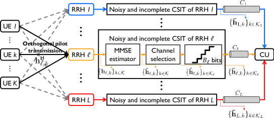
Figure 1: An illustration of noisy-and-incomplete CSI acquisition model. In our model, each RRH estimates the noisy channels, selects a few strongest channels, and quantizes the selected channels to meet the finite-rate fronthaul capacity.

MMSE channel estimation per RRH: Thanks to channel reciprocity in TDD mode, the $\ell$th RRH estimates downlink channel ${\bf h}_{\ell,k}$ by estimating the uplink channel vector ${\bf h}_{\ell,k}^{\sf H}$. Under the premise that each user sends orthogonal pilot sequences with length $\tau\geq K$, the minimum mean square error (MMSE) estimation of ${\bf h}_{\ell,k}$, i.e., ${\bf\hat{h}}_{\ell,k}=\left[{\hat{h}}_{\ell,k}^{1},\ldots,{\hat{h}}_{\ell,k}^{N}\right]^{\sf T}$, is given by

$${\bf\hat{h}}_{\ell,k}={\bf h}_{\ell,k}+{\bf e}_{\ell,k},$$ (2)

where ${\bf e}_{\ell,k}=\left[e_{\ell,k}^{1},\ldots,e_{\ell,k}^{N}\right]^{\sf T}$ is the estimation error vector. Assuming the Gaussian noise in the channel estimation, ${\bf e}_{\ell,k}$ is distributed by zero-mean Gaussian with covariance matrix ${\bf\Phi}_{\ell,k}=\mathbb{E}\left[{\bf e}_{\ell,k}{\bf e}_{\ell,k}^{\sf H}\right]\in\mathbb{C}^{N\times N}$, and it is statistically independent of ${\bf\hat{h}}_{\ell,k}$. Assuming that $p^{{\sf ul}}$ is the uplink pilot transmission power, the channel estimation error covariance matrix is given as a function of spatial covariance matrix ${\bf R}_{\ell,k}$, large-scale fading coefficient $\beta_{\ell,k}$, pilot length $\tau$, and pilot transmission power $p^{{\sf ul}}$ [hoydis2011massive, yin2013coordinated]:

$${\bf\Phi}_{\ell,k} ={\beta}_{\ell,k}{\bf R}_{\ell,k}-{\beta}_{\ell,k}^{2}{\bf R}_{\ell,k}\left({\beta}_{\ell,k}{\bf R}_{\ell,k}+\frac{\sigma^{2}}{\tau p^{\sf ul}}{\bf I}_{N}\right)^{-1}{\bf R}_{{\ell},k}.$$ (3)

Channel selection: We present two channel selection methods using 1) instantaneous CSI and 2) average received signal power at the RRHs. First, using the MMSE channel estimator, RRH $\ell\in\mathcal{L}$ has knowledge of noisy versions of channel vectors, i.e., $\{{\bf\hat{h}}_{\ell,1},\ldots,{\bf\hat{h}}_{\ell,K}\}$. Sending all estimated channel vectors perfectly from the RRH to BBU is infeasible under a finite-rate fronthaul constraint. To compress CSI information, we consider a simple channel selection method. The key idea is to choose the best $U_{\ell}(\leq K)$ channel vectors in the order of the channel gains. Let ${\bf\hat{h}}_{\ell,\pi_{\ell}(k)}$ be the estimated channel vector of the $\ell$th RRH with the $k$th largest channel gain, where $\pi_{\ell}(k)\in\mathcal{K}=\{1,\ldots,K\}$ be the index function such that $\|{\bf\hat{h}}_{\ell,\pi_{\ell}(1)}\|_{2}^{2}\geq\|{\bf\hat{h}}_{\ell,\pi_{\ell}(2)}\|_{2}^{2}\geq\cdots\geq\|{\bf\hat{h}}_{\ell,\pi_{\ell}(K)}\|_{2}^{2}$. Then, each RRH sends the top-$U_{\ell}$ channel vectors, i.e., $\left\{{\bf\hat{h}}_{\ell,k}\right\}$ for $k\in\mathcal{K}_{\ell}=\{\pi_{\ell}(1),\ldots,\pi_{\ell}(U_{\ell})\}$ to BBU, where $U_{\ell}$ is chosen as a function of the fronthaul link capacity $C_{\ell}$. For instance, the fronthaul capacity is extremely limited, RRH $\ell$ can select $U_{\ell}=1$, implying that the best user channel only is sent to BBU. For ease of explanation, we define a subset RRHs that has knowledge of the channel vector for user $k$ by $\mathcal{L}_{k}=\{\ell~{}|~{}k\in\mathcal{K}_{\ell},\forall\ell\}\subset\mathcal{L}$. This index set will be used in the sequel.

In addition, to reduce the CSI acquisition overhead, we propose a simple strategy that estimates the channels for a few strongest channel links in the received power at RRHs. Specifically, each RRH periodically measures the uplink received power of all users, and selects $U_{\ell}(\leq K)$ users in the order of received power at RRH $\ell$ for $\ell\in\mathcal{L}$. Then, RRHs perform the channel estimation to acquire CSI for the selected users, and send the limited CSI to the BBU to generate a precoding solution. To validate the effect of this limited CSI acquisition strategy, we compare the ergodic sum-spectral efficiency performance with the case of using full CSI acquisition at RRHs in Section VI.

Channel quantization: The selected estimated channel, $\left\{{\bf\hat{h}}_{\ell,\pi_{\ell}(1)},\ldots,{\bf\hat{h}}_{\ell,\pi_{\ell}(U_{\ell})}\right\}$, is quantized by using a simple uniform scalar (element-wise) quantizer with $B_{\ell}$ bits resolution. Then, the quantized CSI is sent to BBU via a finite rate fronthaul link $C_{\ell}$ bits per channel use. We assume that the quantization is performed independently across different antennas per RRH, ${{\hat{h}}}_{\ell,k}^{n}$ and ${{\hat{h}}}_{\ell,k}^{m}$ for $n\neq m$. This element-wise uniform quantization method is not optimal because it ignores the statistical correlation effect among the channel coefficients across antennas and RRHs [park2013joint, park2014fronthaul]. Nevertheless, we ignore the spatial correlation effects in the quantization error because their impacts are negligible when using a few-bit quantizer, and we shall focus on this quantization technique because it is more practically relevant from an implementation perspective.

Using standard rate-distortion theory [mezghani2007modified, zhang2016mixed, gersho2012vector], we model the quantization process for the estimated channel of the $n$th antenna at the $\ell$th RRH as

$${\bar{h}}_{\ell,k}^{n} ={\hat{h}}_{\ell,k}^{n}+q_{\ell,k}^{n},\quad\forall k\in\mathcal{K}_{\ell},$$ (4)

where $q_{\ell,k}^{n}$ is the quantization noise of ${\hat{h}}_{\ell,k}^{n}$ which is assumed to be the complex Gaussian with zero-mean and variance $\mathbb{E}[|q_{\ell,k}^{n}|^{2}]={\sigma}^{2}_{q_{\ell,k}^{n}}$, i.e., $q_{\ell,k}^{n}\sim\mathcal{CN}\left({0},{\sigma}^{2}_{q_{\ell,k}^{n}}\right)$. When using the uniform scalar quantizer with $B_{\ell}\geq 6$ bits, it has shown in [mezghani2007modified, gersho2012vector] that the variance of quantization noise is tightly approximated as

$${\sigma}^{2}_{q_{\ell,k}^{n}} \simeq\frac{\pi\sqrt{3}}{2}2^{-2B_{\ell}}\mathbb{E}\left[|\hat{h}_{\ell,k}^{n}|^{2}\right]$$

$$=\frac{\pi\sqrt{3}}{2}2^{-2B_{\ell}}\left[{\beta}_{\ell,k}^{2}{\bf R}_{\ell,k}\left({\beta}_{\ell,k}{\bf R}_{\ell,k}+\frac{\sigma^{2}}{\tau p^{\sf ul}}{\bf I}_{N}\right)^{-1}{\bf R}_{{\ell},k}\right]_{n,n}.$$ (5)

Therefore, the quantized signals $\{{\bar{h}}_{\ell,\pi_{\ell}(1)}^{1},\ldots,{\bar{h}}_{\ell,\pi_{\ell}(1)}^{N},\ldots,{\bar{h}}_{\ell,\pi_{\ell}(U_{\ell})}^{N}\}$, each with $2B_{\ell}$ bits, are reliably delivered from BBU to the $\ell$th RRH with the rate of

$$\sum_{k\in\mathcal{K}_{\ell}}\sum_{n=1}^{N}I({\bar{h}}_{\ell,k}^{n};{\hat{h}}_{\ell,k}^{n}) =\sum_{k\in\mathcal{K}_{\ell}}\sum_{n=1}^{N}\log_{2}\left(1+\frac{\mathbb{E}\left[|\hat{h}_{\ell,k}^{n}|^{2}\right]}{{\sigma}^{2}_{q_{\ell,k}^{n}}}\right)$$

$$\simeq U_{\ell}N\log_{2}\left(1+\frac{2}{\pi\sqrt{3}}2^{2B_{\ell}}\right),$$ (6)

where the first equality follows from the differential entropy of complex Gaussian random variables ${\bar{h}}_{\ell,k}^{n}\sim\mathcal{CN}\left(0,\mathbb{E}\left[|\hat{h}_{\ell,k}^{n}|^{2}\right]+{\sigma}^{2}_{q_{\ell,k}^{n}}\right)$ and ${\hat{h}}_{\ell,k}^{n}\sim\mathcal{CN}\left(0,{\sigma}^{2}_{q_{\ell,k}^{n}}\right)$, and the second approximation holds from ${\sigma}^{2}_{q_{\ell,k}^{n}}\simeq\frac{\pi\sqrt{3}}{2}2^{-2B_{\ell}}\mathbb{E}\left[|\hat{h}_{\ell,k}^{n}|^{2}\right]$ in (5). When $B_{\ell}$ is sufficiently large, i.e., $B_{\ell}\geq 3$, it boils down to

$$U_{\ell}N\log_{2}\left(1+\frac{2}{\pi\sqrt{3}}2^{2B_{\ell}}\right) \simeq U_{\ell}N\log_{2}\left(\frac{2}{\pi\sqrt{3}}2^{2B_{\ell}}\right)$$

$$=U_{\ell}N\left\{\log_{2}\left(2^{2B_{\ell}}\right)-\log_{2}\left(\frac{\pi\sqrt{3}}{2}\right)\right\}$$

$$=U_{\ell}N\left(2B_{\ell}-1.444\right).$$ (7)

Assuming the equal quantization bit allocation strategy per antenna, RRH requires to select the maximum number of quantization bits $B$ to minimize ${\sigma}^{2}_{{q}_{\ell,k}^{n}}$, while ensuring the fronthaul capacity constraint of $U_{\ell}N\log_{2}\left(1+\frac{2}{\pi\sqrt{3}}2^{2B_{\ell}}\right)\leq C_{\ell}$. This condition leads to the choice of the number of quantization bits per fronthaul link

$$B_{\ell}^{\star}=\left\lfloor\frac{1}{2}\log_{2}\left(\frac{\pi\sqrt{3}}{2}\left(2^{\frac{C_{\ell}}{U_{\ell}N}}-1\right)\right)\right\rfloor.$$ (8)

When we denote ${\bf q}_{\ell,k}=\left[q_{\ell,k}^{1},\ldots,q_{\ell,k}^{N}\right]^{\sf T}$, the covariance matrix becomes $\mathbb{E}\left[{\bf q}_{\ell,k}{\bf q}_{\ell,k}^{\sf H}\right]={\bf Q}_{\ell,k}(B_{\ell})\simeq{\sf diag}\left({\sigma}^{2}_{{q}_{\ell,k}^{1}},\ldots,{\sigma}^{2}_{{q}_{\ell,k}^{N}}\right)$. By setting $B_{\ell}^{\star}$ as in (8), it is possible to meet the fronthaul capacity constraints for a given number of antennas and selected users $U_{\ell}$. If the quantization bit $B_{\ell}$ is fixed, to satisfy the constraint, one may alternatively choose $U_{\ell}^{\star}$ such that

$$U_{\ell}^{\star}=\left\lfloor\frac{C_{\ell}}{N\log_{2}\left(1+\frac{2}{\pi\sqrt{3}}2^{2B_{\ell}}\right)}\right\rfloor.$$ (9)

As a result, our CSI compression strategy, including the channel selection and quantization, can meet the fronthaul capacity constraint $C_{\ell}$ by flexibly choosing both the number of selected channels to share $U_{\ell}$ and the number of quantization bits to represent each selected channel values $B_{\ell}$. The effect of the trade-off between $U_{\ell}$ and $B_{\ell}$ for given $C_{\ell}$ will be shown numerically in the simulation section.

II-B Downlink Transmission with Limited Fronthaul Capacity

Using the proposed CSI estimation and compression strategy, BBU has noisy-and-incomplete CSIT $\{{\bf\bar{h}}_{\ell,k}\}_{\ell\in\mathcal{L},k\in\mathcal{K}_{\ell}}$. This subsection explains how BBU performs joint precoding to send downlink data symbols using this partial downlink channel knowledge.

Linear precoding: Let $s_{k}[t]$ and ${\bf f}_{\ell,k}$ be a downlink transmit symbol to user $k$ in the $t$th time slot and the linear precoding vector being used at the $\ell$th RRH to deliver $s_{k}[t]$. When the coherence time interval is given by $\tau_{c}$, we assume that $s_{k}[t]$ is drawn from a complex Gaussian codebook with the average power $P=\mathbb{E}\left[|s_{k}[t]|^{2}\right]$ in the $t$th time slot where $t\in[\tau_{c}]$. Then, the precoded complex downlink signal of RRH $\ell$ is represented by a linear superposition of precoder ${{\bf f}_{\ell,k}}s_{k}[t]$ for $k\in\mathcal{K}$, i.e.,

$${\bf x}_{\ell}[t]=\sum_{k\in\mathcal{K}}{\bf f}_{\ell,k}s_{k}[t],~{}~{}~{}~{}\forall\ell\in\mathcal{L}.$$ (10)

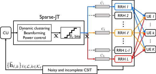
Figure 2: The proposed sparse-JT for C-RANs.

Precoded signal quantization: In the similar manner of the channel quantization process, the precoded signal ${\bf x}_{\ell}[t]$ is quantized using a simple uniform scalar quantizer with ${\bar{B}}_{\ell}$ bits quantization levels. The transmitted signal of the $n$th antenna at RRH $\ell$ after applying the quantization is given by

$${\bar{x}}_{\ell}^{n}[t] ={x}_{\ell}^{n}[t]+{v}_{\ell}^{n}[t],$$ (11)

where ${v}_{\ell}^{n}[t]$ is the quantization noise of ${x}_{\ell}^{n}[t]$ which is assumed to be the complex Gaussian with zero-mean and variance $\mathbb{E}[|{v}_{\ell}^{n}[t]|^{2}]={\sigma}^{2}_{{v}_{\ell}^{n}}$, i.e., ${v}_{\ell}^{n}[t]\sim\mathcal{CN}\left({0},{\sigma}^{2}_{{v}_{\ell}^{n}}\right)$. From [mezghani2007modified, zhang2016mixed, gersho2012vector], the quantization noise variance when using the ${\bar{B}}_{\ell}$ bits uniform scalar quantizer with ${\bar{B}}_{\ell}\geq 6$ is tightly approximated as

$${\sigma}^{2}_{{v}_{\ell}^{n}}\simeq\eta_{\ell}({\bar{B}}_{\ell})\cdot\mathbb{E}\left[|x_{\ell}^{n}[t]|^{2}\right]=\eta_{\ell}({\bar{B}}_{\ell})\cdot\left(\sum_{k=1}^{K}|f_{\ell,k}^{n}|^{2}P\right),$$ (12)

where $\eta_{\ell}({\bar{B}}_{\ell})=\frac{\pi\sqrt{3}}{2}2^{-2B_{\ell}}$. Therefore, the quantized signals $\left\{{\bar{x}}_{\ell}^{1}[t],\ldots,{\bar{x}}_{\ell}^{N}[t]\right\}$, each with $2{\bar{B}}_{\ell}$ bits, are reliably delivered from BBU to the $\ell$th RRH with the rate of

$$\sum_{n=1}^{N}I({\bar{x}}_{\ell}^{n}[t];{x}_{\ell}^{n}[t])=\sum_{n=1}^{N}\log\left(1+\frac{\sum_{k=1}^{K}|f_{\ell,k}^{n}|^{2}P}{{\sigma}^{2}_{{v}_{\ell}^{n}}}\right)\simeq N\log\left(1+\eta_{\ell}({\bar{B}}_{\ell})^{-1}\right).$$ (13)

Using the rate expression in (13), BBU selects the number of quantization bits $B_{\ell}$ to minimize ${\sigma}^{2}_{{v}_{\ell}^{n}}$ while ensuring the fronthaul capacity constraint such that

$${\bar{B}}_{\ell}^{\star}=\left\lfloor\frac{1}{2}\log_{2}\left(\frac{\pi\sqrt{3}}{2}\left(2^{\frac{C_{\ell}}{N}}-1\right)\right)\right\rfloor.$$ (14)

It is remarkable that the quantization bits ${\bar{B}}_{\ell}^{\star}$ derived in (14) allows us to satisfy the fronthaul capacity constraints regardless of precoding strategies because it alters the quantization levels as a function of the norm of precoding vectors to meet the constraint. From the relationship between ${\sigma}^{2}_{{v}_{\ell}^{n}}$ and ${\bar{B}}_{\ell}$ in (12), the effective quantization noise variance ${\sigma}^{2}_{{v}_{\ell}^{n}}$ reduces by designing the precoding vectors $\sum_{k=1}^{K}|f_{\ell,k}^{n}|^{2}$ for each $n\in[N]$ and $\ell\in\mathcal{L}$ with a small norm. Therefore, our precoding strategy aims at minimizing the norm of precoding vectors $\sum_{k=1}^{K}|f_{\ell,k}^{n}|^{2}$ for each $n\in[N]$ and $\ell\in\mathcal{L}$. To explicitly represent ${\sigma}^{2}_{{v}_{\ell}^{n}}$ as a function of precoding vectors, we define a precoding matrix for RRH $\ell\in\mathcal{L}$ by ${\bf F}_{\ell}=[{\bf f}_{\ell,1},\ldots,{\bf f}_{\ell,K}]$. Then, the covariance matrix for the quantization noise in a compact form is

$${\bf V}_{\ell}({\bf F}_{\ell},{\bar{B}}_{\ell}^{\star})=\mathbb{E}[{\bf v}_{\ell}[t]{\bf v}_{\ell}[t]^{\sf H}]=P\cdot\eta_{\ell}^{\star}({\bar{B}}_{\ell}^{\star})\cdot{\sf diag}\left(\sum_{k=1}^{K}|f_{\ell,k}^{1}|^{2},\ldots,\sum_{k=1}^{K}|f_{\ell,k}^{N}|^{2}\right),$$ (15)

where $\eta_{\ell}^{\star}({\bar{B}}_{\ell}^{\star})=\frac{\pi\sqrt{3}}{2}2^{-2{\bar{B}}_{\ell}^{\star}}$ and ${\bf v}_{\ell}[t]=\left[v_{\ell}^{1}[t],\ldots,v_{\ell}^{N}[t]\right]^{\sf T}$.

Ergodic spectral efficiency: The received signal of the $k$th user is

$$y_{k}[t] =\sum_{\ell=1}^{L}{\bf h}_{\ell,k}^{\sf H}{\bf\bar{x}}_{\ell}[t]+z_{k}[t]$$

$$=\sum_{\ell=1}^{L}{\bf h}_{\ell,k}^{\sf H}{\bf f}_{\ell,k}s_{k}[t]+\sum_{\ell=1}^{L}\sum_{i\neq k}{\bf h}_{\ell,k}^{\sf H}{\bf f}_{\ell,i}s_{i}[t]+\sum_{\ell=1}^{L}{{\bf h}_{\ell,k}^{\sf H}{\bf v}_{\ell}}[t]+z_{k}[t],$$ (16)

where $z_{k}[t]$ is the noise signal of the $k$th user, which is distributed as $\mathcal{CN}(0,\sigma^{2})$. Then, the signal-to-interference-plus-noise ration (SINR) of the $k$th user is defined as

$${\sf SINR}_{k} =\frac{\left|\sum_{\ell=1}^{L}{\bf h}_{\ell,k}^{\sf H}{\bf f}_{\ell,k}\right|^{2}}{\sum_{i\neq k}\left|\sum_{\ell=1}^{L}{\bf h}_{\ell,k}^{\sf H}{\bf f}_{\ell,i}\right|^{2}+\sum_{\ell=1}^{L}{\bf h}_{\ell,k}^{\sf H}{\bf V}_{\ell}({\bf F}_{\ell},{\bar{B}}_{\ell}^{\star}){\bf h}_{\ell,k}/P+\sigma^{2}/P}.$$ (17)

With noisy-and-incomplete CSIT, ${\bf\bar{H}}=\{{\bf\bar{h}}_{\ell,k}\}_{\ell\in\mathcal{L},k\in\mathcal{K}_{\ell}}$, the BBU estimates the instantaneous spectral efficiency of the $k$th downlink user, i.e.,

$$R_{k}\left({\bf\bar{H}}\right)=\mathbb{E}_{{\bf H}|{\bf\bar{H}}}\left[\log_{2}\left(1+{\sf SINR}_{k}\right)|{\bf\bar{H}}\right],\quad k\in\mathcal{K}_{\ell},$$ (18)

where the expectation is taken over both channel estimation and quantization errors. Therefore, by taking the expectation over every fading states, we obtain the ergodic spectral efficiency

$${\bar{R}}_{k}=\left(1-\frac{\tau_{u}+\tau_{d}}{\tau_{c}}\right)\mathbb{E}_{{\bf\bar{H}}}\left[R_{k}\left({\bf\bar{H}}\right)\right]=\left(1-\frac{\tau_{u}+\tau_{d}}{\tau_{c}}\right)\mathbb{E}\left[\log_{2}\left(1+{\sf SINR}_{k}\right)\right],$$ (19)

where $\tau_{u}$ and $\tau_{d}$ denote the uplink and downlink channel training lengths respectively.

III Sum-Spectral Efficiency Maximization Problem

In this section, we shall formulate a sum-spectral efficiency maximization problem with noisy-and-incomplete CSIT under a sparsely active RRH constraint. To accomplish this, we first derive a lower bound of the instantaneous spectral efficiency. Then, we formulate the spare precoding optimization problem that maximizes the obtained lower bound of the instantaneous spectral efficiency under the sparsely active RRH constraint.

III-A A Lower Bound of Instantaneous Spectral Efficiency

We begin by rewriting the received signal in (16) in terms of the noisy-and-quantized CSIT at BBU, i.e., ${\bf h}_{\ell,k}={\bf\hat{h}}_{\ell,k}+{\bf e}_{\ell,k}={\bf\bar{h}}_{\ell,k}+{\bf e}_{\ell,k}+{\bf q}_{\ell,k}$, which yields

$$y_{k}[t] =\sum_{\ell=1}^{L}\left[\left({\bf\bar{h}}_{\ell,k}+{\bf e}_{\ell,k}+{\bf q}_{\ell,k}\right)^{\sf H}\left({\bf f}_{\ell,k}s_{k}[t]+\sum_{i\neq k}{\bf f}_{\ell,i}s_{i}[t]+{\bf v}_{\ell}[t]\right)\right]+z_{k}[t]$$

$$=\sum_{\ell=1}^{L}{\bf\bar{h}}_{\ell,k}^{\sf H}{\bf f}_{\ell,k}s_{k}[t]+\sum_{\ell=1}^{L}\sum_{i\neq k}{\bf\bar{h}}_{\ell,k}^{\sf H}{\bf f}_{\ell,i}s_{i}[t]+{\tilde{z}}_{k}[t],$$ (20)

where ${\tilde{z}}_{k}[t]$ is the effective noise term, i.e.,

$${\tilde{z}}_{k}[t]=\sum_{\ell=1}^{L}\sum_{i=1}^{K}\left({\bf e}_{\ell,k}+{\bf q}_{\ell,k}\right)^{\sf H}{\bf f}_{\ell,i}s_{i}[t]+\sum_{\ell=1}^{L}\left({\bf\bar{h}}_{\ell,k}+{\bf e}_{\ell,k}+{\bf q}_{\ell,k}\right)^{\sf H}{\bf v}_{\ell}[t]+z_{k}[t].$$ (21)

Unfortunately, the effective noise ${\tilde{z}}_{k}[t]$ is non-Gaussian because the product of two Gaussian random variables $s_{i}[t]$ and ${\bf e}_{\ell,k}+{\bf q}_{\ell,k}$ is not Gaussian. Harnessing the generalized mutual information [yoo2006capacity, medard2000effect, lapidoth2002fading, ding2010maximum], in which the non-Gaussian noise is simply modeled as the Gaussian noise with a proper moment matching, we characterize a lower bound of the instantaneous spectral efficiency [choi2018joint, choi2019joint]. To accomplish this, we need to compute the variance of the effective noise ${\tilde{z}}_{k}[t]$. Since $\mathbb{E}[{\tilde{z}}_{k}[t]]=0$, the effective noise variance is

$${\tilde{\sigma}}^{2}_{k} =\mathbb{E}[|{\tilde{z}}_{k}[t]|^{2}]$$

$$=P\sum_{\ell=1}^{L}\sum_{i=1}^{K}{\bf f}_{\ell,i}^{\sf H}\mathbb{E}\left[{\bf e}_{\ell,k}{\bf e}_{\ell,k}^{\sf H}+{\bf q}_{\ell,k}{\bf q}_{\ell,k}^{\sf H}+{\bf e}_{\ell,k}{\bf q}_{\ell,k}^{\sf H}+{\bf q}_{\ell,k}{\bf e}_{\ell,k}^{\sf H}\right]{\bf f}_{\ell,i}+\sum_{\ell=1}^{L}\mathbb{E}\left[{\bf h}_{\ell,k}^{\sf H}{\bf v}_{\ell}[t]{\bf v}_{\ell}[t]^{\sf H}{\bf h}_{\ell,k}\right]+\sigma^{2}$$ (22)

$$=P\sum_{\ell=1}^{L}\sum_{i=1}^{K}{\bf f}_{\ell,i}^{\sf H}\left({\bf\Phi}_{\ell,k}+{\bf Q}_{\ell,k}(B_{\ell}^{\star})\right){\bf f}_{\ell,i}+\sum_{\ell=1}^{L}{\sf Tr}\left({\bf R}_{\ell,k}{\bf V}_{\ell}({\bf F}_{\ell},{\bar{B}}_{\ell}^{\star})\right)+\sigma^{2},$$ (23)

where the last equality follows from the fact that the channel estimation error noise is independent of the channel quantization noise, i.e., $\mathbb{E}\left[{\bf e}_{\ell,k}{\bf q}_{\ell,k}^{\sf H}\right]={\bf 0}$. Invoking this effective noise variance, a lower bound of instantaneous spectral efficiency when using noisy-and-incomplete CSIT is

$$\sum_{k=1}^{K}R_{k}^{\sf low}=\sum_{k=1}^{K}\log_{2}\left(1+\frac{\left|\sum_{\ell=1}^{L}{\bf\bar{h}}_{\ell,k}^{\sf H}{\bf f}_{\ell,k}\right|^{2}}{\sum_{i\neq k}\left|\sum_{\ell=1}^{L}{\bf\bar{h}}_{\ell,k}^{\sf H}{\bf f}_{\ell,i}\right|^{2}+{\tilde{\sigma}}_{k}^{2}/P}\right).$$ (24)

The sum-spectral efficiency in (24) is the estimate of the instantaneous sum-spectral efficiency with limited channel knowledge, which will be used to find a joint solution for user clustering, beamforming, and power allocation in the sequel.

III-B Sparsely Active RRH Constraint

Let $S$ be the maximum number of active RRHs per the joint transmission, and it is assumed to be smaller than a total number of RRHs $L$ in the network, i.e., $S\leq L$. We also define an index set of active RRHs as

$$\mathcal{A}=\{\ell:\|{\bf x}_{\ell}[t]\|_{2}^{2}\neq 0\}\subset\mathcal{L}.$$ (25)

It is true that $\sum_{k=1}^{K}\|{\bf f}_{\ell,k}\|_{2}^{2}>0$ if $\|{\bf x}_{\ell}[t]\|_{2}^{2}\neq 0$. Using this relation, to perform sparse-JT, we need to design the precoding vectors to satisfy the following group-sparsity condition:

$$\sum_{\ell=1}^{L}{\bf 1}_{\left\{\sum_{k=1}^{K}\|{\bf f}_{\ell,k}\|_{2}^{2}>0\right\}}\leq S,$$ (26)

where ${\bf 1}_{{\mathcal{C}}}$ is an indicator function such that ${\bf 1}_{{\mathcal{C}}}=1$ if an event ${\mathcal{C}}$ is true and ${\bf 1}_{{\mathcal{C}}}=0$ otherwise. Our optimization task is to identify precoding vectors, $\{{\bf f}_{\ell,k}\}_{\ell\in\mathcal{L},k\in\mathcal{K}}$, to maximize the lower bound of the instantaneous spectral efficiency (24) under the group-sparsity constraints (26). This optimization problem is formulated as

$$\mathscr{P}^{1}:~{}~{}~{}~{} {\underset{\{{\bf f}_{\ell,k}\}_{\ell\in\mathcal{L},k\in\mathcal{K}}}{\text{arg~{}max}}}~{}\sum_{k=1}^{K}\log_{2}\left(1+\frac{\left|\sum_{\ell=1}^{L}{\bf\bar{h}}_{\ell,k}^{\sf H}{\bf f}_{\ell,k}\right|^{2}}{\sum_{i\neq k}\left|\sum_{\ell=1}^{L}{\bf\bar{h}}_{\ell,k}^{\sf H}{\bf f}_{\ell,i}\right|^{2}+{\tilde{\sigma}}_{k}^{2}/P}\right),$$ (27a)

$$\text{subject to}~{}~{}\sum_{k=1}^{K}\|{\bf f}_{\ell,k}\|_{2}^{2}\leq(1+{\eta}_{\ell}^{\star}({\bar{B}}_{\ell}^{\star}))^{-1},~{}~{}~{}\forall\ell\in\mathcal{L},$$ (27b)

$$~{}~{}~{}~{}~{}~{}~{}~{}~{}~{}~{}~{}~{}\sum_{\ell=1}^{L}{\bf 1}_{\left\{\sum_{k=1}^{K}\|{\bf f}_{\ell,k}\|_{2}^{2}>0\right\}}\leq S,$$ (27c)

where the $L$ inequalities in (27b) correspond to the per-RRH power constraint, $\mathbb{E}[\|{\bf\bar{x}}_{\ell}\|_{2}^{2}]\leq P$. Obtaining the global optimal solution for this optimization problem even without a group-sparsity constraint is highly non-trivial, because the objective function is non-convex with respective to precoding vectors. Additionally, the group-sparsity constraint makes the problem a combinatorial optimization.

III-C Reformation to a Generalized Sparse-PCA Problem

We explain how the optimization problem (27) can be reformulated in a generalized sparse-PCA problem. The following proposition elucidates the connection between them.

Proposition 1.

Let ${\bf f}\in\mathbb{C}^{LNK\times 1}$ be a network-wide precoding vector by concatenating all precoding vectors to form a large-dimensional optimization variable, namely,

$${\bf{f}} =[\underbrace{{\bf{f}}_{1,1}^{\sf{H}},\cdots,{\bf{f}}_{L,1}^{\sf{H}}}_{{\bf f}_{1}^{\sf H}},\cdots,\underbrace{{\bf{f}}_{1,k}^{\sf{H}},\cdots,{\bf{f}}_{L,k}^{\sf{H}}}_{{\bf f}_{k}^{\sf H}},\cdots,\underbrace{{\bf{f}}_{1,K}^{\sf{H}},\cdots,{\bf{f}}_{L,K}^{\sf{H}}}_{{\bf f}_{K}^{\sf H}}]^{\sf{H}}\in\mathbb{C}^{LNK\times 1}.$$ (28)

We also define large-dimensional positive semidefinite matrices ${\bf A}_{k}\in\mathbb{C}^{LNK\times LNK}$ and ${\bf B}_{k}\in\mathbb{C}^{LNK\times LNK}$ such that ${\bf f}^{\sf H}{\bf A}_{k}{\bf f}$ and ${\bf f}^{\sf H}{\bf B}_{k}{\bf f}$ are the total received power and the interference power received at user $k$th, which are

$${\bf A}_{k} ={\bf I}_{K}\otimes\left({\bf\bar{h}}_{k}{\bf\bar{h}}_{k}^{\sf H}+{\bf\Phi}_{k}+{\bf Q}_{k}\left(B_{\ell}^{\star}\right)\right)+\frac{\sum_{\ell=1}^{L}{\sf Tr}\left({\bf R}_{\ell,k}{\bf V}_{\ell}({\bf F}_{\ell},{\bar{B}}_{\ell}^{\star})\right)+\sigma^{2}}{P\cdot\sum_{\ell=1}^{L}(1+{\eta}_{\ell}^{\star}({\bar{B}}_{\ell}^{\star}))^{-1}}{\bf I}_{LNK}\in\mathbb{C}^{LNK\times LNK},$$ (29)

$${\bf B}_{k} ={\bf A}_{k}-{\bf a}_{k}{\bf a}_{k}^{\sf T}\otimes{\bf\bar{h}}_{k}{\bf\bar{h}}_{k}^{\sf H}\in\mathbb{C}^{LNK\times LNK},$$ (30)

where ${\bf\bar{h}}_{k}=\left[{{\bf\bar{h}}}_{1,k}^{\sf H},\ldots,{{\bf\bar{h}}}_{L,k}^{\sf H}\right]^{\sf H}$, ${\bf\Phi}_{k}={\sf diag}\left({\bf\Phi}_{1,k},\ldots,{\bf\Phi}_{L,k}\right)$, and ${\bf Q}_{k}(B_{\ell}^{\star})={\sf diag}({\bf Q}_{1,k}(B_{\ell}^{\star}),\ldots,{\bf Q}_{L,k}(B_{\ell}^{\star}))$. Then, the optimization problem $\mathscr{P}^{1}$ is equivalent to the following problem:

$$\mathscr{P}^{2}:~{}~{}~{}~{} {\underset{{\bf f}\in\mathbb{C}^{LNK\times 1}}{\text{arg~{}max}}}~{}\log_{2}\left(\prod_{k=1}^{K}\frac{{{\bf f}^{\sf H}{\bf A}_{k}{\bf f}}}{{{\bf f}^{\sf H}{\bf B}_{k}{\bf f}}}\right),$$ (31a)

$$\text{subject to}\sum_{\ell=1}^{L}{\bf 1}_{\left\{\sum_{k=1}^{K}\|{\bf f}_{\ell,k}\|_{2}^{2}>0\right\}}\leq S.$$ (31b)

Proof:

The key idea is that we reformulate the objective function (27a) to a product of the Rayleigh quotients by representing the optimization variables in a high dimensional space as in [choi2018joint, choi2019joint, han2020distributed]. Specifically, using the aggregated vectors, ${\bf\bar{h}}_{k}$ and ${\bf f}_{k}$, we arrange the received signal representation of the $k$th user in (16) to a compact form as

$$y_{k}[t]={\bf\bar{h}}_{k}^{\sf H}{\bf f}_{k}s_{k}[t]+\sum_{i\neq k}^{K}{\bf\bar{h}}_{k}^{\sf H}{\bf f}_{i}s_{i}[t]+{\tilde{z}}_{k}[t],$$ (32)

where the effective noise ${\tilde{z}}_{k}[t]$ is defined with the aggregated channel estimation and quantization error vectors ${\bf e}_{k}=\left[{{\bf e}}_{1,k}^{\sf H},\ldots,{{\bf e}}_{L,k}^{\sf H}\right]^{\sf H}$, ${\bf q}_{k}=\left[{{\bf q}}_{1,k}^{\sf H},\ldots,{{\bf q}}_{L,k}^{\sf H}\right]^{\sf H}$ and ${\bf v}[t]=\left[{\bf v}_{1}[t]^{\sf H},\ldots,{\bf v}_{L}[t]^{\sf H}\right]^{\sf H}$ as

$${\tilde{z}}_{k}[t]=\sum_{i=1}^{K}\left({\bf e}_{k}-{\bf q}_{k}\right)^{\sf H}{\bf f}_{i}s_{i}[t]+{\bf h}_{k}^{\sf H}{\bf v}[t]+z_{k}[t],$$ (33)

Then, the variance of effective noise can be rewritten with respective to the aggregate precoding vectors as

$${\tilde{\sigma}}_{k}^{2}=\mathbb{E}\left[|{\tilde{z}}_{k}[t]^{2}|\right]=P\sum_{i=1}^{K}{\bf f}_{i}^{\sf H}\left({\bf\Phi}_{k}+{\bf Q}_{k}\left(B_{\ell}^{\star}\right)\right){\bf f}_{i}+\sum_{\ell=1}^{L}{\sf Tr}\left({\bf R}_{\ell,k}{\bf V}_{\ell}({\bf F}_{\ell},{\bar{B}}_{\ell}^{\star})\right)+\sigma^{2}.$$ (34)

Note that ${\bf e}_{\ell,k}$, ${\bf q}_{\ell,k}$, ${\bf\Phi}_{\ell,k}$, and ${\bf Q}_{\ell,k}(B_{\ell}^{\star})$ becomes zero vectors and matrices when $\ell\notin\mathcal{L}_{k}$. Furthermore, we relax the per-RRH power constraint, $\sum_{k=1}^{K}\|{\bf f}_{\ell,k}\|_{2}^{2}\leq(1+{\eta}_{\ell}^{\star}({\bar{B}}_{\ell}^{\star}))^{-1}$ for all $\ell\in\mathcal{L}$, to the network-wide sum-power constraint, i.e., $\sum_{\ell=1}^{L}\sum_{k=1}^{K}\|{\bf f}_{\ell,k}\|_{2}^{2}=\|{\bf f}\|_{2}^{2}=\sum_{\ell=1}^{L}(1+{\eta}_{\ell}^{\star}({\bar{B}}_{\ell}^{\star}))^{-1}$. This relaxation reduces $L$ equality constraints to a single equality constraint. Then, harnessing the large-dimensional network-wide precoding vector ${\bf f}$, our objective function in (27a) is written in a form of the product of Rayleigh quotients as

$$\sum_{k=1}^{K}\log_{2}\left(1+\frac{\left|\sum_{\ell=1}^{L}{\bf\bar{h}}_{\ell,k}^{\sf H}{\bf f}_{\ell,k}\right|^{2}}{\sum_{i\neq k}\left|\sum_{\ell=1}^{L}{\bf\bar{h}}_{\ell,k}^{\sf H}{\bf f}_{\ell,i}\right|^{2}+{\tilde{\sigma}}_{k}^{2}/P}\right) =\sum_{k=1}^{K}\log_{2}\left(\frac{\sum_{i=1}^{K}\left|\sum_{\ell=1}^{L}{\bf\bar{h}}_{\ell,k}^{\sf H}{\bf f}_{\ell,i}\right|^{2}+{\tilde{\sigma}}_{k}^{2}/P}{\sum_{i\neq k}^{K}\left|\sum_{\ell=1}^{L}{\bf\bar{h}}_{\ell,k}^{\sf H}{\bf f}_{\ell,i}\right|^{2}+{\tilde{\sigma}}_{k}^{2}/P}\right)$$

$$=\log_{2}\left(\prod_{k=1}^{K}\frac{{{\bf f}^{\sf H}{\bf A}_{k}{\bf f}}}{{{\bf f}^{\sf H}{\bf B}_{k}{\bf f}}}\right).$$ (35)

Since the objective function (35) is invariant to scale of any real value $\alpha\in\mathbb{R}$ on ${\bf f}$, i.e,. $\log_{2}\left(\prod_{k=1}^{K}\frac{{{\bf f}^{\sf H}{\bf A}_{k}{\bf f}}}{{{\bf f}^{\sf H}{\bf B}_{k}{\bf f}}}\right)=\log_{2}\left(\prod_{k=1}^{K}\frac{{\alpha{\bf f}^{\sf H}{\bf A}_{k}\alpha{\bf f}}}{{\alpha{\bf f}^{\sf H}{\bf B}_{k}\alpha{\bf f}}}\right)$, we discard the sum-power constraint to further simplify the optimization problem. Therefore, the sum-spectral efficiency maximization problem in (27) is equivalent to (31), which completes the proof. ∎

This reformulated optimization problem is interesting because it can be interpreted with a lens through a generalized sparse-PCA problem in machine learning [zou2006sparse]. To shed further light on the significance of the reformulation in (31), we will provide a more detailed explanation at the end of this section.

III-D Tractable Relaxation for Group-Sparsity Constraint

Unfortunately, the reformulated optimization problem (31) in Proposition 1 is still a non-convex and combinatorial optimization problem. In this section, we take a non-convex approximation to relax the group-sparsity constraint in a tractable quadratic form.