Analyzing states beyond full synchronization on hypergraphs requires methods beyond projected networks

Abstract

A common approach for analyzing hypergraphs is to consider the projected adjacency or Laplacian matrices for each order of interactions (e.g., dyadic, triadic, etc.). However, this method can lose information about the hypergraph structure and is not universally applicable for studying dynamical processes on hypergraphs, which we demonstrate through the framework of cluster synchronization. Specifically, we show that the projected network does not always correspond to a unique hypergraph structure. This means the projection does not always properly predict the true dynamics unfolding on the hypergraph. Additionally, we show that the symmetry group consisting of permutations that preserve the hypergraph structure can be distinct from the symmetry group of its projected matrix. Thus, considering the full hypergraph is required for analyzing the most general types of dynamics on hypergraphs. We show that a formulation based on node clusters and the corresponding edge clusters induced by the node partitioning, enables the analysis of admissible patterns of cluster synchronization and their effective dynamics. Additionally, we show that the coupling matrix projections corresponding to each edge cluster synchronization pattern, and not just to each order of interactions, are necessary for understanding the structure of the Jacobian matrix and performing the linear stability calculations efficiently.

I Introduction

The framework of dynamical systems on dyadic networks provides a useful tool for modeling the behavior of many systems, including those from biological, social, and engineered realms [barrat2008dynamical, danon2011networks, rhoden2012self, porter2020nonlinearity+, curto2019relating]. However, some systems have higher order non-additive interactions which require going beyond dyadic interactions [bick2021higherorder, battiston2020networks]. Hypergraphs are a natural extension of dyadic networks that allow the study of a wider range of systems by capturing higher-order interactions. Naturally, adding higher order interactions requires modifying tools from systems with dyadic interactions to be applicable to dynamics on hypergraphs and also developing new tools to analyze the system’s behavior.

There are several ways higher order dynamics can be defined. Namely, dynamics can be defined on the nodes interacting via hyperedges of different orders [skardal2019abrupt, skardal2020memory, gambuzza2020master, zhang2020unified, xu2020bifurcation, landry2020effect, lucas2020multi, skardal2020higher]. Alternatively, especially if the dynamics is defined on a simplicial complex, the dynamical signals can be defined on simplices of different dimensions [millan2020explosive, ghorbanchian2021higher, deville2021consensus]. Here, we take the former approach. Specifically, we consider dynamics on undirected hypergraphs, where the evolution of each node depends on the state of its neighbors via dyadic and higher order interactions. Additionally, we assume that some sets of nodes within the system have similar internal dynamics, and some sets of edges have similar coupling forms. We specifically study cluster synchronization where groups of oscillators in the system have fully synchronized trajectories, but distinct groups follow distinct trajectories. The framework of cluster synchronization is useful for analyzing intricate patterns of synchronization in dynamical systems on hypergraphs and it illustrates the difference between analysis based on full hypergraph considerations and those based on dyadic projections.

To study synchronization in higher order systems, the generalization of the dyadic graph adjacency and Laplacian matrices are useful tools. Several ways to generalize these matrices from the perspective of node interactions have been recently proposed [carletti2020dynamical, lucas2020multi, de2021phase, gambuzza2020master]. These generalizations are based on projecting the higher order edges onto dyadic cliques and finding the adjacency or Laplacian of a resulting network for each order of interactions. Specifically, the projections of this form are sufficient to formulate stability conditions for full synchronization on undirected hypergraphs [gambuzza2020master, de2021phase, lucas2020multi] and chemical hypergraphs [mulas2020coupled] or even some cases of cluster synchronization, such as non-intertwined cluster synchronization [zhang2020unified]. A downside of hypergraph projection is the non-applicability of such analysis to more intricate types of synchronization dynamics in higher order systems. In this manuscript, we demonstrate that the hypergraph projection description is not sufficient for analyzing cluster synchronization in the most general case.

First we show that the projection is not always in one-to-one correspondence with the original higher order system. In other words, several non-isomorphic hypergraphs can have the same projection onto a dyadic network. Specifically we demonstrate that distinct hypergraphs can have the same projection, yet the effective interactions on the hypergraphs can be distinct even for the same pattern of cluster synchronization (i.e., which nodes follow the same trajectory, and which do not). It is these effective interactions between the clusters that determine the dynamical behavior. Projections are sensitive enough for capturing full synchronization dynamics and its stability properties, but do not necessarily capture more intricate patterns of synchronization.

We next compare the symmetries of the full hypergraph with the symmetries of its dyadic projections to show that the hypergraph does not always admit the same cluster synchronization patterns as one would deduce from its dyadic projections. Symmetry considerations, namely the orbits of the symmetry group of the system (as well as its subgroups), can be used to determine some of the admissible cluster synchronization states [golubitsky2003symmetry, pecora2014cluster]. While the symmetries of the projected hypergraph are often in direct correspondence with the symmetries of the original hypergraph [gambuzza2020master], we demonstrate that for some topologies, some of the symmetries of the projected network do not preserve the hypergraph structure (also discussed in Ref.[mulas2020hypergraph]).

Our final contribution is showing how projected networks can be used for stability calculations. In systems with purely dyadic interactions, cluster synchronization states do not necessarily arise from symmetries alone [stewart2003symmetry]. They can also arise from more general balanced equivalence relations. This is also the case for systems with higher order interactions, both for Laplacian-like coupling [salova2021h1, salova2021code] and more general couplings discussed in this manuscript. To analyze general cluster synchronization patterns whether they arise from symmetries or more generally from equitable partitions, we define the concept of edge clusters with each edge cluster corresponding to a specific edge synchronization pattern. We demonstrate that one needs to define a separate projected adjacency matrix for each edge synchronization pattern and hyperedge order to fully capture the structure of the Jacobian matrix used for linear stability analysis.

Linear stability calculations can be simplified using simultaneous block diagonalization [zhang2020symmetry]. We demonstrate that the set of matrices that need to be simultaneously block diagonalized to analyze cluster synchronization on hypergraphs includes the projected adjacency matrices for each edge pattern of synchronization for interactions beyond dyadic (discussed in detail in LABEL:subsec:_app). In contrast, stability analysis for dyadic interactions does not require tracking the individual edge synchronization patterns.

The rest of the manuscript is organized as follows. Section II provides the basic formulation for dynamical systems on undirected hypergraphs and the general conditions for cluster synchronization in such systems based on node and edge partitions. Section III demonstrates that the hypergraph projection does not always allow us to unambiguously reconstruct the original hypergraph up to an isomorphism, which can produce misleading predictions for the effective dynamics of cluster synchronization states. In Section IV we consider symmetries and show that some of the orbital partitions of the projected hypergraph do not describe the admissible cluster synchronization states of the original hypergraph, thus projected adjacency matrices are not always sufficient to determine the admissible patterns of synchronization on hypergraphs. LABEL:sec:_stab demonstrates that the projected hypergraph adjacency matrices combined with the cluster synchronization indicator matrices are not sufficient to fully represent the structure of the Jacobian and simplify its analysis in the case of the most general hypergraph structure and pattern of synchronization. Instead, we show how to use projections corresponding to different cluster synchronization patterns to perform the linear stability analysis. Finally, we discuss our results and future directions in LABEL:sec:_conclusion.

II Background: cluster synchronization oh hypergraphs

II.1 Hypergraph structure and dynamics

First, we define the general form of the dynamics on hypergraphs that is being considered. A hypergraph is defined by a set of $N$ nodes and a set of hyperedges $e_{j}\in\mathcal{E}$. In this work, we focus on undirected hyperedges. Let $\mathcal{E}_{i}\subset\mathcal{E}$ be the set of hyperedges that contain node $i$. Each hyperedge $e_{j}\in\mathcal{E}_{i}$ contains a set of nodes $e_{j}=\{i,j_{1},...,j_{m-1}\}$. The order of the hyperedge $e_{j}$ is $m$, which is the number of nodes including $i$ that are part of it. Thus, $m=2$ corresponds to dyadic edges, $m=3$ to triadic edges, etc.

Using notation similar to Ref.[de2021phase], we can express the evolution of the state of each node in the system, $x_{i}\in R^{n}$, as:

$$\dot{x}_{i}=F_{i}(x_{i})+\sum\limits_{e\in\mathcal{E}_{i}}G_{e}(x_{i},x_{e\backslash i}).$$ (1)

Here, the function $F_{i}(x_{i})$ describes the evolution of uncoupled nodes, and the function $G_{e}(x_{i},x_{e\backslash i})$ is a coupling function corresponding to the influence of the hyperedge $e$ on node $i$, where $x_{i}$ is the state of the node $i$ itself, and $x_{e\backslash i}$ is the state of the rest of the edge. This setup is general, including the case when the interaction hypergraph is a simplicial complex which has the additional requirement that each subset of nodes in the hyperedge forms a hyperedge of lower order.

Often, some degree of homogeneity is present within the nodal dynamics, $F_{i}(x_{i})$, of different nodes $i$ as well as in the coupling dynamics, $G_{e}(x_{i},x_{e\backslash i})$. In that case, one can use the hypergraph structure to find nontrivial partitions into sets of nodes that can fully synchronize. In the simplest case, all the self-dynamics are characterized by the same function $F$ and the coupling dynamics of a given order $m$ are characterized by the same function $G^{(m)}$. In that case, it is sufficient to consider adjacency structures (e.g., adjacency tensors) with binary entries.

The exact higher order adjacency structure can be defined in terms of the collection of $m$ incidence matrices $I^{(m)}$, one for each order $m$. Let $\mathcal{E}^{(m)}_{i}$ be the set of hyperedges of order $m$ containing the node $i$. Then, the nonzero elements of the incidence matrix are $[I^{(m)}]_{i,e}=1$ if $e\in\mathcal{E}^{(m)}_{i}$. Additionally, we assume undirected coupling, so $[I^{(m)}]_{i,e}=1$ for all $i\in e$.

With these simplifications, the dynamics of Eq. 1 can be expressed as:

$$\dot{x}_{i}= F(x_{i})+\sum\limits_{m=2}^{d}\sigma^{(m)}\sum\limits_{e\in\mathcal{E}^{(m)}}[I^{(m)}]_{i,e}G^{(m)}(x_{i},x_{e\backslash i}),$$ (2)

where due to undirected coupling we assume that the function $G^{(m)}(x_{i},x_{e\backslash i})$ is invariant under any reordering of nodes in $x_{e\backslash i}$.

In Ref.[salova2021h1], we cover the stability analysis in the case of Laplacian and Laplacian-like coupling. Here, we assume more general undirected coupling. In the case of undirected coupling, the presence of the hyperedge $\{i_{1},...,i_{k},...,i_{m}\}$ providing input to node $i_{1}$ via the coupling function $G^{(m)}$, s.t. $\dot{x}_{i_{1}}=...+G^{(m)}(x_{i_{1}},...,x_{i_{k}},...,x_{i_{m}})$, implies that hyperedge affects $x_{i_{k}}$ via the same coupling function, s.t. $\dot{x}_{i_{k}}=...+G^{(m)}(x_{i_{k}},...,x_{i_{1}},...,x_{i_{m}})$. Additionally, the coupling function responsible for providing input into node $x_{i_{1}}$ has to be invariant with respect to permutations of the elements corresponding to the nodes providing this input within a hyperedge, namely, $G^{(m)}(x_{i_{1}},...,x_{i_{k}},...,x_{i_{k^{\prime}}},...)=G^{(m)}(x_{i_{1}},...,x_{i_{k^{\prime}}},...,x_{i_{k}},...)$. For a concrete example of triadic coupling, consider the extension of the Kuramoto model to triadic interactions presented in Ref.[PhysRevResearch.2.023281], with $G^{(3)}(x_{i},x_{j},x_{k})=K\sin(\theta_{j}+\theta_{k}-2\theta_{i})$, where we set the coupling strengths $\sigma^{(3)}$ to be identical for all triadic edges. First, we note that $G^{(3)}(x_{i},x_{j},x_{k})=G^{(3)}(x_{i},x_{k},x_{j})$. In addition, for the coupling to be undirected, we require that $I_{i,e}=I_{j,e}=I_{k,e}$, where the edge $e$ consists of nodes $i$, $j$, and $k$.

II.2 Bipartite representation of a hypergraph

While incidence matrices are a useful and compact representation of the hypergraph structure, sometimes it is helpful to deal with square matrices instead. Thus, hypergraphs represented via a bipartite graph will be useful for much of the analysis herein. The adjacency matrix $\mathcal{M}$ of the bipartite representation of a hypergraph is of the form:

$$\mathcal{M}=\begin{pmatrix}0_{N\times N}&I_{N\times M}\\ I^{T}_{N\times N}&0_{M\times M}\end{pmatrix},$$ (3)

where $N$ is the number of nodes in the hypergraph, $M$ is the number of edges, and $I$ is its incidence matrix. While this matrix is less compact than the incidence matrix, this bipartite graph representation allows the use of standard dyadic interaction tools in analyzing systems with higher order interactions, as $\mathcal{M}$ is a square matrix.

An important caveat here is that one needs to additionally take into account that the elements of $\mathcal{M}$ represent the relations between nodes and edges, and not simply the interactions between the nodes. This is discussed in more detail in Section III in the context of hypergraph isomorphism and Section IV in relation to admissible patterns of cluster synchronization.

II.3 Dyadic projections of hypergraphs

A common way to analyze hypergraph structure and full synchronization dynamics is by using the projection of the hypergraph structure onto a dyadic coupling matrix for each order of interaction. Depending on the type of the coupling function, either an adjacency or Laplacian projection can be used. In several recent publications [carletti2020dynamical, lucas2020multi, de2021phase, gambuzza2020master], the projected matrices for each order of interactions are defined as:

$$\mathcal{A}^{(m)}=I^{(m)}[I^{(m)}]^{T}-\mathcal{D}^{(m)},$$ (4)

where $[\mathcal{D}^{(m)}]_{ii}=\sum\limits_{j}I^{(m)}_{ij}$ and has zero off-diagonal elements.

This projection is useful in analyzing, for instance, the stability of full synchronization in systems with higher order interactions, by either forming an aggregate projection matrix with different edge orders being assigned different weights [de2021phase, carletti2020dynamical, lucas2020multi], or considering projected Laplacians in case of noninvasive coupling [gambuzza2020master]. However, in some cases, this projection loses information about the original hypergraph even for a given order of interactions (e.g., triadic), as discussed in Section III and Section IV. Additionally, these projections are insufficient for cluster synchronization analysis, which is why we need to define such a projection for every edge pattern of synchronization, as discussed in LABEL:sec:_stab.

II.4 Admissible patterns of cluster synchronization on hypergraphs

While projection matrices are useful in analyzing full synchronization, collective behavior of coupled dynamical systems is more complicated when the nodes are not fully synchronized. Often, it is useful to analyze these behaviors using the framework of cluster synchronization, where the nodes in the same clusters $C_{i}$ are fully synchronized due to receiving the same dynamical input, but their behavior is distinct from all the other clusters $C_{j}$. Cluster synchronization can arise as a form of symmetry breaking in systems with identical nodes and edges (or hyperedges of the same order) that allow full synchronization. However, it can also be present in systems with multiple node and edge types, such as multilayer networks, in which full synchronization solutions are not admissible.

Patterns of cluster synchronization have been extensively analyzed for systems with dyadic interactions [belykh2008cluster, pecora2014cluster, pecora2017discovering, cho2017stable, salova2020decoupled], with a few recent advances to higher order systems. Cluster synchronization of coupled map lattices on chemical hypergraphs was recently analyzed in Ref.[bohle2021coupled], but the setup is distinct from the general structure and dynamics considered in this manuscript. Stability of cluster synchronization in systems like the one in Eq. 2 is analyzed in Ref.[zhang2020unified]. However, the question of admissibility of different patterns is not discussed there, and the analysis is limited to non-intertwined clusters. Finally, cluster synchronization on hypergraphs is briefly discussed in Ref.[gambuzza2020master]. However, the reference only discusses the patterns of synchronization arising from symmetries and does not discuss the ones arising from more general partitions (e.g., discussed in Ref.[salova2021h1] and later herein). Additionally, the conditions for symmetry-based clusters in Ref.[gambuzza2020master] may not be sufficient for general hypergraphs, and additional checks must be performed as discussed in detail in Section IV.

In this section, we demonstrate how to find the admissible cluster synchronization patterns by partitioning the nodes into node clusters, and the edges into edge clusters based on the node clusters those edges span. The framework is similar to that in Ref.[salova2021h1], but we do not restrict the coupling functions to Laplacian-like coupling. As an example of cluster synchronization, consider Fig. 1(a). The hypergraph structure shown on the left admits a cluster synchronization pattern with two node clusters, shown in purple and teal. Each purple node $p$ obtains input from two hyperedges, one of the form $C^{(3)}_{ppp}$ (containing three nodes in the purple cluster) and one $C^{(3)}_{ptt}$. Each teal node $t$ gets input from two edges of the form $C^{(3)}_{ptt}$. We will index the node clusters as $C_{j}$ (where $j$ can refer to a cluster number or a cluster “color”). Here, the node clusters are $C_{1}=C_{p}=\{1,2,3\}$ and $C_{2}=C_{t}=\{4,5,6\}$. The edge clusters induced by node partition (i.e., hyperedges which span equivalent node clusters, and, therefore, have equivalent node trajectories) are denoted by $C_{j}^{(m)}$. In this example, $C^{(3)}_{1}=C^{(3)}_{ppp}=\{[1,2,3]\}$ and $C^{(3)}_{2}=C^{(3)}_{ptt}=\{[1,4,5],[2,4,6],[3,5,6]\}$. The bipartite graph in Fig. 1(a) (right) demonstrates the relations between nodes (circles) and edges (triangles). The bipartite graph makes it clear that there are two triadic edge clusters ($C^{(3)}_{1}$ shown in olive and $C^{(3)}_{2}$ shown in yellow) induced by the node clusters.

The cluster synchronization pattern in Fig. 1(a) is not the only admissible pattern. Fig. 1 (a-d) shows four distinct example partitions, using direct hypergraph representation (left column) and its bipartite representation (right column).

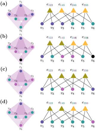
Figure 1: Synchronization patterns in hypergraphs. Left column: hypergraph, right column: equivalent bipartite representation. [(a-d)] Distinct cluster synchronization patterns.

Mathematically, the condition for an admissible cluster synchronization state based on the incidence matrix is

$$\sum\limits_{e_{j}\in C^{(m)}_{k}}I^{(m)}_{ij}=\sum\limits_{e_{j}\in C^{(m)}_{k}}I^{(m)}_{i^{\prime}j}$$ (5)

where $i,i^{\prime}\in C_{l}$, and the summation is performed over all the columns of $I^{(m)}$ corresponding to the edges in the $k$th edge cluster of order $m$, denoted by $C_{k}^{(m)}$. Eq. 5 has to hold for all the orders of interaction and edge clusters, unless the specific form of the coupling function makes some edge clusters irrelevant to cluster synchronization admissibility (e.g., fully synchronized hyperedges in Ref.[salova2021h1]).

The effective interactions between different clusters are contained in the quotient hypergraph, where

$$I^{(m)}_{\text{eff}}=\mathcal{P}_{n}I^{(m)}\mathcal{(}{\mathcal{P}}_{e}^{(m)})^{T},$$ (6)

where $\mathcal{P}_{n}$ ($K\times N$) and $\mathcal{P}_{e}^{(m)}$ ($K_{m}\times N$) are the indicator matrices corresponding to node and edge partitions, and $I^{(m)}$ is the $m$th order incidence matrix. The nonzero elements of the indicator matrices $\mathcal{P}_{n}$ and $\mathcal{P}_{e}^{(m)}$ are defined by $[\mathcal{P}_{n}]_{i,j}=1$ if node $i$ belongs to node cluster $C_{j}$, and $[\mathcal{P}_{e}^{(m)}]_{i,j}=1$ if the $m$th order edge $i$ belongs to the $m$th order edge cluster $C^{(m)}_{j}$.

Note that Eq. 5 can be easily modified to handle the case where there are different types of nodes and hyperedges in the system. If distinct node types are present, only the ones within the same type are expected to fully synchronize. To put it in the form of Eq. 5, we can form a trivial incidence matrix $I^{(1)}$, where $I^{(1)}_{i}=I^{(1)}_{j}$ if and only if the nodes $i$ and $j$ are of the same type, and add those incidence matrices to the set that needs to be tested in Eq. 5. If distinct hyperedge types are present, Eq. 5 has to hold for each edge interaction order $m$ and for each edge type.

Equivalently, the bipartite graph adjacency matrix (Eq. 3) can be used to partition nodes and edges into clusters using the methods applicable to systems with dyadic interactions (even for systems with different types of nodes and hyperedges). Importantly, since we distinguish between nodes and edges, they need to be partitioned into clusters separately (corresponding to the case of two distinct types of nodes in systems with dyadic interactions). It is also important to note that for each node partition obtained from the bipartite representation, only the coarsest edge partition is properly identified. For instance, Fig. 2 demonstrates two partitions admissible on the bipartite graph, whose structure corresponds to the hypergraph with six nodes (shown as circles in the bipartite graph) and four triadic edges (shown as shaded triangles). However, only one of the resulting partitions (Fig. 2 top right) is an admissible partition of the nodes and hyperedges of the hypergraph itself. Fig. 2 bottom right shows that partitioning the bipartite representation can misidentify the edge partitions induced by the node partitions. In this case, all hyperedges contain the same nodes (purple, teal, violet), and thus have to belong to the same edge cluster, although the bipartite representation divides them into two edge clusters.

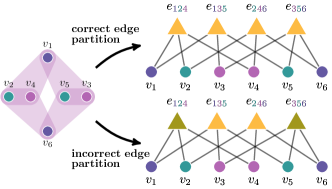
Figure 2: Left: cluster synchronization pattern on a hypergraph. Right: equitable partitions of the corresponding bipartite network. Only the top partition represents the correct node and edge partition of the hypergraph. In the bottom partition, the hyperedges $e_{124}$ and $e_{356}$ are incorrectly assigned into a cluster distinct from that containing $e_{135}$ and $e_{246}$, even though all the hyperedges consist of one violet, one purple, and one teal node.

III Hypergraph dyadic projection: loss of information on structure and effective dynamics

Hypergraph projections can be used to analyze fully synchronized states and their stability [de2021phase, gambuzza2020master]. However, this tool is not always useful in analyzing general dynamics on hypergraphs, including cluster synchronization. Initial results obtained in Ref.[de2021phase] led its authors to conjecture that it is possible to create a hypergraph projection (with the adjacency matrix calculated as a weighted sum of terms defined in Eq. 4) that fully preserves the information about the hypergraph structure. However, we show the projection as defined in Eq. 4 does not necessarily correspond to a unique hypergraph. In fact, these distinct hypergraphs that get mapped onto the same single projection do not even have to be isomorphic, as we show next in Section III.1. As a result, sometimes the hypergraphs with the same node clusters and projected adjacency matrix have distinct quotient hypergraphs, and thus different cluster synchronization dynamics.

III.1 Example: non-isomorphic hypergraphs with distinct effective dynamics but identical dyadic projection

Identical hypergraphs, as well as isomorphic hypergraphs, produce identical dynamical behavior, including cluster synchronization. However, the hypergraphs that map onto the same projected network are not necessarily identical or isomorphic, and therefore can produce distinct dynamical behavior despite having the same projection. This can be investigated computationally, especially since the problem can be considered on a single order of higher order interactions at the time, because distinct orders can be distinguished in the projection.

To obtain hypergraphs that are not isomorphic, but which have the same projected dyadic adjacency matrix, it is sufficient to find two distinct incidence matrices, $I_{1}^{(m)}$ and $I_{2}^{(m)}$, that satisfy

$$I_{1}^{(m)}[{I}_{1}^{(m)}]^{T}-D^{(m)}={I}_{2}^{(m)}[{I}_{2}^{(m)}]^{T}-D^{(m)}=\mathcal{A}^{(m)},$$ (7)

with no nontrivial permutational matrix $P$ satisfying

$$P(\mathcal{M}_{1}+\mathcal{R})=(\mathcal{M}_{2}+\mathcal{R})P,$$ (8)

where $\mathcal{M}_{1}$ and $\mathcal{M}_{2}$ are the respective adjacency matrices corresponding to the bipartite graph representation of the original hypergraphs. Here, $\mathcal{R}$ is a diagonal matrix whose purpose is to avoid permuting nodes with edges. It has diagonal entries $\mathcal{R}_{ii}=\alpha$ if $i\leq N$ and $\mathcal{R}_{ii}=\beta$ if $i>N$. In numerical calculations, $\alpha$ and $\beta$ can be set to be distinct random numbers.

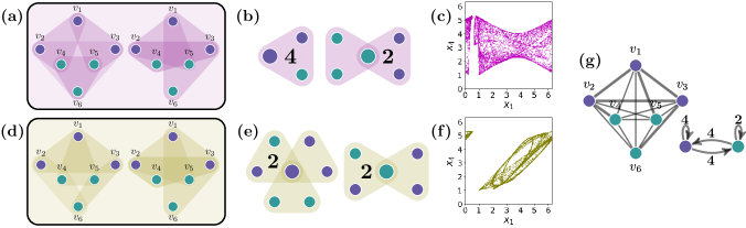
Figure 3: Synchronization patterns in hypergraphs. Teal and violet node colors correspond to distinct node synchronization clusters. [(a) and (d)] Hypergraph structure of two distinct hypergraphs (violet box (a) and olive box (d)) containing the union of hypergraphs shown on the left and on the right. The left hypergraphs in (a) and (d) are distinct, but isomorphic to each other. The right hypergraphs in these boxes are fully identical. [(b) and (e)] Distinct quotient hypergraphs for cases (a) and (d) respectively. [(c) and (f)] State of node $4$ ($x_{4}$) vs state of node $1$ ($x_{1}$) using Section III.1 dynamics evolved for $10^{4}$ time steps for the two-cluster state on hypergraphs (a) and (d) respectively. Node $1$ belongs to the violet cluster, node $4$ belongs to the teal cluster. (g) The same projected network (left) and its quotient network (right) results for both cases (a) and (d). Thick lines correspond to edges of weight two, and thin lines correspond to those of weight one.

As an example, consider two distinct hypergraphs with triadic interactions, each with six nodes and seven hyperedges. The first is shown in the box shaded in purple in Fig. 3(a), and the second in the box shaded in olive in Fig. 3(d). Both Fig. 3(a) and Fig. 3(d) are the union of the two simpler hypergraphs shown in the respective boxes. The hypergraphs in the left column of Fig. 3(a) and (d) are isomorphic but distinct, whereas the right column hypergraphs are identical. Note, the full hypergraphs in Fig. 3(a) and (d) are not isomorphic. The graph isomorphism problem is notoriously complicated. However, we used the networkx.is_isomorphic Python package [hagberg2008exploring] to verify that indeed $\mathcal{M}_{1}+\mathcal{R}$ corresponding to Fig. 3(a) is not isomorphic to $\mathcal{M}_{2}+\mathcal{R}$ corresponding to Fig. 3(d). We denote their incidence matrices by $I_{1}$ and $I_{2}$. The corresponding projected dyadic graph for both of the above hypergraphs, containing edges of weight $1$ and $2$ (shown in thin and thick lines respectively), is demonstrated in Fig. 3(g). Its adjacency matrix is

$$\mathcal{A}^{(3)} =I_{1}^{(3)}(I_{1}^{(3)})^{T}-\mathcal{D}^{(3)}=I_{2}^{(3)}(I_{2}^{(3)})^{T}-\mathcal{D}^{(3)}$$

$$=\begin{pmatrix}0&1&1&2&2&2\\ 1&0&1&2&1&1\\ 1&1&0&1&2&1\\ 2&2&1&0&2&1\\ 2&1&2&2&0&1\\ 2&1&1&1&1&0\\ \end{pmatrix}.$$ (9)

Thus, the conditions from Eq. 7 hold: two non-isomorphic hypergraphs, Fig. 3(a) and (d), s.t. no nontrivial permutation satisfies Eq. 8 for their bipartite adjacency matrices $\mathcal{M}_{1}$ and $\mathcal{M}_{2}$, have the same projected adjacency matrix.

The fact that non-isomorphic hypergraphs may have the same projected graph has consequences on the cluster synchronization dynamics. Specifically, the inability to reconstruct the original hypergraph may lead to an ambiguity in effective dynamics in a hypergraph, even if the node assignment into clusters is the same between the two hypergraphs. As an example, consider the coloring of nodes on Fig. 3. In all its subfigures, teal and violet nodes represent distinct clusters. This cluster assignment is admissible in both hypergraphs in Fig. 3(a) and (d). The corresponding quotient hypergraphs are shown respectively in Fig. 3(b) and (e). These hypergraphs represent the effective dynamics of each type of node (teal and violet). As very clearly visible in Fig. 3, these quotient hypergraphs are qualitatively different. The dynamics on each type of nodes in case of Fig. 3(b) is:

$$\dot{x}_{p} =F(x_{p})+4G^{(3)}(x_{p},x_{p},x_{t}),$$

$$\dot{x}_{t} =F(x_{t})+G^{(3)}(x_{t},x_{t},x_{t})+2G^{(3)}(x_{t},x_{p},x_{p}),$$ (10)

whereas in case of Fig. 3(e) it is:

$$\dot{x}_{p}= F(x_{p})+2G^{(3)}(x_{p},x_{p},x_{t})$$

$$+G^{(3)}(x_{p},x_{p},x_{p})+G(x_{p},x_{t},x_{t}),$$

$$\dot{x}_{t}= F(x_{t})+2G^{(3)}(x_{t},x_{p},x_{t})+G^{(3)}(x_{t},x_{p},x_{p}),$$ (11)

leading to distinct behaviors.

To provide a concrete example of distinct trajectories arising from Section III.1 and Section III.1, we consider the discrete time dynamics:

$$x_{i}^{t+1}=F(x_{i}^{t})+\sigma^{(3)}\sum\limits_{e\in\mathcal{E}^{(m)}}[I^{(3)}]_{i,e}G^{(3)}(x_{e\backslash i}^{t}),$$ (12)

where $x_{i}^{t}$ is the state of the node $i$ at time $t$, and the self evolution and coupling functions are defined as:

$$F(x_{i}^{t}) =\alpha\dfrac{1-\cos(x_{i}^{t})}{2}+\dfrac{\pi}{6},$$

$$G^{(3)}(x_{j}^{t},x_{k}^{t}) =\dfrac{1-\cos(x_{j}^{t}+x_{k}^{t})}{2}.$$ (13)

This oscillator dynamics is the optoelectronic dynamics defined in Ref.[cho2017stable] with added triadic interactions. We also use this dynamics in LABEL:subsec:_stab. Here, we chose the parameters $\alpha=0.5$ and $\sigma^{(3)}=1.5$. Fig. 3(c) demonstrates the dynamics of two clusters (teal and violet) on the hypergraph shown in Fig. 3(a), and Fig. 3(f) demonstrates the dynamics of these clusters on the hypergraph shown in Fig. 3(d). The dynamics of the two-cluster state are clearly distinct for these different hypergraph topologies with the same projected network.

Here, we covered one of the mechanisms that leads to non-isomorphic hypergraphs having the same projected adjacency matrix. Namely, it requires picking two isomorphic hypergraphs, and breaking the isomorphism by adding the same set of additional hyperedges. Clearly, if additional identical interactions of any order are present in both hypergraphs, Eq. 7 still holds and the hypergraphs will have the same projection.

Note that in case of complete synchronization, distinct hypergraphs with the same dyadic projection produce the same effective behavior, so this phenomenon only arises for more complicated dynamical states.

III.2 Does loss of information from the projection occur frequently in randomly selected hypergraphs?

To estimate if the information loss from projecting the hypergraph is frequent for a given number of nodes ($n_{\text{nodes}}$) and hyperedges ($n_{\text{edges}}$), we investigate how often the condition in Eq. 7 holds for pairs of hypergraphs with hyperedges added at random.

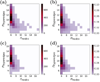
Figure 4: (a) Number and (b) fraction of pairs of non-isomorphic hypergraphs sharing the same projection for a given number of nodes and triadic hyperedges. (c) Number and (d) fraction of pairs of non-isomorphic fully connected hypergraphs sharing the same projection.

It is known that bipartite network projections may exhibit data loss. In fact, it was shown that in some cases, non-isomorphic bipartite networks with incidence matrices $I_{1}$ and $I_{2}$ can have identical projections corresponding to node and edge interactions, i.e., $I_{1}I_{1}^{T}=I_{2}I_{2}^{T}$ and $I_{1}^{T}I_{1}=I_{2}^{T}I_{2}$, but those cases are rare [kirkland2018two]. Here, we consider a similar problem in the context of hypergraphs, but only require the node interaction projections to be identical. In fact, for the example discussed in Fig. 3, $I_{1}^{T}I_{1}\neq I_{2}^{T}I_{2}$. This leaves us a wider range of options to explore. On the other hand, since we consider hypergraph projections where different edge orders can be distinguished, we only focus on matrices $I$ with constant column sums, where these sums equal to the edge order. This restriction narrows down the types of incidence matrices we consider.

Here, we focus on the case of triadic interactions on hypergraphs. First, we create $10,000$ random hypergraphs by randomly selecting with replacement three distinct nodes that will be connected by a hyperedge $n_{\text{edges}}$ times for each of the hypergraphs consisting of $n_{\text{nodes}}$ nodes. We note that the resulting hypergraphs may have duplicate edges, isolated nodes, or several connected components. We accept this since in real hypergraphs, more than one edge order can be present, so the nodes that are isolated for a specific interaction order may not be isolated when all orders of interactions are considered. But we also compare the results to those considering only fully connected hypergraphs. Then, we remove the “duplicate” isomorphic hypergraphs. Finally, we find the non-isomorphic hypergraphs satisfying Eq. 7 and calculate the number and fractions of such pairs for each number of nodes and hyperedges. The results calculated for small numbers of nodes and hyperedges are presented in Fig. 4. We note that while these hypergraphs are not common, they could still occur as motifs in larger hypergraphs. For example, consider two identical hypergraphs. Adding different extra hyperedges to the same subset of their nodes, s.t. those hyperedges satisfy Eq. 7 makes the whole hypergraph satisfy Eq. 7, producing two hypergraphs that are not isomorphic but have the same projection.

IV Symmetry differences between hypergraphs and their dyadic projections

Structural symmetries of hypergraphs and dyadic networks determine some of the types of synchronization patterns admissible in the system and assist in determining their stability. We demonstrate that in some cases, there are symmetries of the projected adjacency matrix that are not the symmetries of the original hypergraph.

Specifically, consider the permutations of each order of interactions defined in Ref.[gambuzza2020master]

$$P\mathcal{L}^{(m)}=\mathcal{L}^{(m)}P,$$ (14)

or, equivalently,

$$P\mathcal{A}^{(m)}=\mathcal{A}^{(m)}P,$$ (15)

where the permutation matrices $P$ satisfying Eq. 15 for each order of interactions form the symmetry group. For the examples studied in Ref.[gambuzza2020master], the resulting symmetry group is associated with cluster synchronization states on simplicial complexes. We demonstrate that is not always the case, both in case of dynamics on simplicial complexes, or, more generally, hypergraphs. While this issue does not arise very often in randomly selected large hypergraphs, it is still important to know that using the conditions in Ref. [gambuzza2020master] to obtain the patterns of cluster synchronization requires an extra step of checking that each specific pattern is admissible on the full hypergraph and not just the projections of every order. Thus, next in Section IV.1, we develop the conditions for cluster synchronization to arise from symmetries that hold for any hypergraph structure.

IV.1 Hypergraph symmetries

Equitable partitions (groupings of nodes into clusters, in which nodes in the same cluster receive the same input from that cluster as well as all the other clusters) give rise to the admissible cluster synchronization states for a given hypergraph structure. Equitable partitions that result from structural symmetries of the hypergraph are called orbital partitions and are a special case of more general equitable partitions [golubitsky2003symmetry, golubitsky2012singularities]. For instance, all the partitions shown in Fig. 1 are orbital partitions, while the ones shown later in LABEL:fig:_equitable are not. Even more flexibility is allowed for Laplacian-like coupling which requires only external equitable partitions (groupings of nodes into clusters, in which nodes in the same cluster receive the same input from all the other clusters, meaning that the hyperedges only containing one type of node cluster, e.g., the edge $e_{123}$ in Fig. 1(a), can be ignored for admissibility purposes), and patterns arising from symmetries are less common in that case [salova2021h1]. In summary, orbital partitions are a subset of equitable partitions, which are the subset of external equitable partitions.

Our focus in this section is structural symmetries. First, we state the algorithm for finding symmetry induced cluster synchronization patterns in systems with dyadic interactions. The automorphism group of the dyadic adjacency matrix $A$ is formed by a set of permutation matrices $P$, s.t. $PA=AP$. Any subgroup of that group can be linked to an admissible cluster synchronization pattern via orbital partitions. Namely, all the subsets of the network nodes that get mapped to themselves (and thus belong to the same cell of the orbital partition) can be completely synchronized [pecora2014cluster]. The approach can be generalized to systems with different types of nodes and interactions, e.g., multilayer networks of coupled oscillators where cluster synchronization requires compatibility between intra- and interlayer symmetries [della2020symmetries].

Symmetries of dyadic projected networks can not be immediately translated to those of a system with higher order interactions similarly to more general equitable partition methods. Instead, one has to consider the full hypergraph and the node and edge permutations simultaneously to assess the hypergraph synchronization patterns from the symmetry perspective. Symmetries, such as the ones analyzed in Ref.[mulas2020hypergraph] for directed hypergraphs, arise from the hypergraph automorphism group with elements $P$ represented as permutation matrices. We formulate the cluster synchronization condition in terms of the symmetries of the undirected hyperedges of each order $m$ as:

$$PI=IP_{\text{edge}}.$$ (16)

Here, $P_{N\times N}$ is a permutation matrix that reorders the nodes, and $[P_{\text{edge}}]_{M\times M}$ corresponds to the permutations of the edge labels if node labels are permuted. These hyperedge permutation matrices are defined as follows:

$$[P_{\text{edge}}]_{e_{i},e_{j}}=[P]_{i_{1}j_{1}}...[P]_{i_{m}j_{m}},$$ (17)

where $e_{i}=\{i_{1},...,i_{m}\}$ and $e_{j}=\{j_{1},...,j_{m}\}$ are the hyperedges. The orbits of the subgroups of the automorphism group with elements $P$ determine the admissible cluster synchronization patterns.

Note that $I$ here is an aggregate matrix combining all the interaction orders. Alternatively, we could consider the incidence matrices for different orders of interactions, $I^{(m)}$, separately. Then, the largest common subgroup of the symmetry groups of all the interaction orders determines the automorphism group of the hypergraph.

As an example, consider the incidence matrix corresponding to the hypergraph structure in Fig. 1

(18)

(19)

(20)

(21)

(22)

(23)

(24)

(25)

Oneofthepairscontainin