Controlling epidemics through optimal allocation of test kits and vaccine doses across networks

Abstract

Efficient testing and vaccination protocols are critical aspects of epidemic management. To study the optimal allocation of limited testing and vaccination resources in a heterogeneous contact network of interacting susceptible, recovered, and infected individuals, we present a degree-based testing and vaccination model for which we use control-theoretic methods to derive optimal testing and vaccination policies. Within our framework, we find that optimal intervention policies first target high-degree nodes before shifting to lower-degree nodes in a time-dependent manner. Using such optimal policies, it is possible to delay outbreaks and reduce incidence rates to a greater extent than uniform and reinforcement-learning-based interventions, particularly on certain scale-free networks.

I Introduction

Limiting the spread of novel pathogens such as SARS-CoV-2 requires efficient testing [1, 2] and quarantine strategies [3], especially when vaccines are not available or effective. Even if effective vaccines become available at scale, their population-wide distribution is a complex and time-consuming endeavor, influenced by, for example, population age-structure [4, 5, 6], vaccine hesitancy [7], and different objectives [8].

Until a sufficient level of immunity within a population is reached, distancing and quarantine policies can also be used to help slow the spread and evolutionary dynamics [9] of infectious diseases. Epidemic modeling and control-theoretic approaches are useful for identifying both efficient testing and vaccination policies. For an epidemic model of SARS-CoV-2 transmission, Pontryagin’s maximum principle (PMP) has been used to derive optimal distancing and testing strategies that minimize the number of COVID-19 cases and intervention costs [10]. Optimal control theory has also been applied to a multi-objective control problem that uses isolation and vaccination to limit epidemic size and duration [11]. Both of these recent investigations describe the underlying infectious disease dynamics through compartmental models without underlying network structure, meaning that all interactions among different individuals are assumed to be homogeneous. For a structured susceptible-infected-recovered (SIR) model, optimal vaccination strategies have been derived for a rapidly spreading disease in a highly mobile urban population using PMP [12]. Complementing these control-theory-based interventions, a recent work [13] developed methods relying on reinforcement learning (RL) to identify infectious high-degree nodes (“superspreaders”) in temporal networks and reduce the overall infection rate with limited medical resources. The application of optimal control methods and PMP to a heterogeneous node-based susceptible-infected-recovered-susceptible (SIRS) model with applications to rumor spreading was studied in [14].

The machine-learning-based interventions of [13] showed that RL is able to outperform intervention policies derived from purely structural node characterizations that are, for instance, based on centrality measures. However, the methods of [13] were applied to rather small networks with a maximum number of nodes of about 400. Here, we focus on a complementary approach by formulating optimal control and RL-based target policies for a degree-based epidemic model [15] that is constrained only by the maximum degree and not by the system size (i.e., number of nodes). Early work by May and Anderson [16] employed such effective degree models to study the population-level dynamics of human immunodeficiency virus (HIV) infections. These degree-based models and later adaptations [17, 18, 19] do not account for degree correlations. Effective degree models for susceptible-infected-susceptible (SIS) dynamics with degree correlations were derived in [20] and applied to SIR dynamics in [21]. A further generalization of these methods to model SIR dynamics with networked and well-mixed transmission pathways was presented in [22]. For a detailed summary of degree-based epidemic models, see [23].

In the next section, we propose and justify a degree-based epidemic, testing, and quarantining model. An optimal control framework for this model is presented in Sec. III and, given limited testing resources, an optimal testing strategy is calculated. We extend the same underlying disease model to include vaccination in Sec. IV and find optimal vaccination strategies that minimize infection given a limited vaccination rate. We summarize and discuss our results and how they depend on network and dynamical features of the model in Sec. V. For comparison, we also present in the Appendix a reinforcement-learning-based algorithm that is able to approximate optimal testing strategies for the model introduced in Sec. II.

II Degree-based epidemic and testing model

For the formulation of optimal testing policies that allocate testing resources to different individuals in a contact network, we adopt an effective degree model of SIR dynamics with testing in a static network of $N$ nodes. Nodes represent individuals, and edges between nodes represent corresponding contacts. Therefore, the degree of a node represents the number of its contacts. If $K$ is the maximum degree across all nodes, we can divide the population into $K$ distinct subpopulations, each of size $N_{k}$ ($k=1,2,\dots,K$) such that all nodes in the $k^{\rm th}$ group have degree $k$. Therefore, $N=\sum_{k=1}^{K}N_{k}$.

In our epidemic model, we distinguish between untested and tested infected individuals. Let $S_{k}(t)$, $I_{k}^{{\rm u}}(t)$, $I_{k}^{{*}}(t)$, and $R_{k}(t)$ denote the numbers of susceptible, untested infected, tested infected, and recovered nodes with degree $k$ at time $t$, respectively. Since these subpopulations together represent the entire population (the total number of nodes $N$), both $N$ and $N_{k}$ are constants in our model. Their values satisfy the normalization condition $S_{k}+I_{k}^{\rm u}+I_{k}^{*}+R_{k}=N_{k}$. The corresponding fractions are

$$s_{k}(t)=S_{k}(t)/N, \quad i_{k}^{\rm u}(t)=I_{k}^{\rm u}(t)/N,$$ (1)

$$i_{k}^{*}(t)=I_{k}^{*}(t)/N, \quad r_{k}(t)=R_{k}(t)/N,$$

such that $\sum_{k}(s_{k}+i_{k}^{\rm u}+i_{k}^{*}+r_{k})=1$. Using an effective-degree approach [16, 22], we describe the evolution of the above subpopulations by

$$\frac{\mbox{d}s_{k}(t)}{\mbox{d}t}= -ks_{k}(t)\sum_{\ell=1}^{K}{P(\ell|k)\over P(\ell)}\big{(}\beta^{\rm u}i_{\ell}^{\rm u}(t)+\beta^{*}i_{\ell}^{*}(t)\big{)},$$ (2)

$$\frac{\mbox{d}i_{k}^{\rm u}(t)}{\mbox{d}t}= ks_{k}(t)\sum_{\ell=1}^{K}{P(\ell|k)\over P(\ell)}\big{(}\beta^{\rm u}i_{\ell}^{\rm u}(t)+\beta^{*}i_{\ell}^{*}(t)\big{)}$$ (3)

$$\hskip 79.6678pt-\gamma^{u}i_{k}^{\rm u}(t)-\frac{f_{k}(t)}{N_{k}}i_{k}^{\rm u}(t),$$

$$\frac{\mbox{d}i_{k}^{*}(t)}{\mbox{d}t}= -\gamma^{*}i_{k}^{*}(t)+\frac{f_{k}(t)}{N_{k}}i_{k}^{\rm u}(t),$$ (4)

$$\frac{\mbox{d}r_{k}(t)}{\mbox{d}t}= \gamma^{\rm u}i_{k}^{\rm u}(t)+\gamma^{*}i_{k}^{*}(t),$$ (5)

where $P(\ell)=N_{\ell}/N$ is the degree distribution and $P(\ell|k)$ is the probability that a chosen node with degree $k$ is connected to a node with degree $\ell$. Our degree-based formulation of SIR dynamics with testing, Eqs. (2)–(5), is an approximation of the full node-based dynamics assuming that nodes of the same degree are equally likely to be infected at any given time [15].

Susceptible individuals become infected through contact with untested and tested infected individuals at rates $\beta^{\rm u}$ and $\beta^{*}$, respectively. Untested and tested infected individuals recover at rates $\gamma^{\rm u}$ and $\gamma^{*}$, respectively. Differences in the recovery rates $\gamma^{\rm u}$ and $\gamma^{*}$ reflect differences in disease severity of and treatment options for untested and tested infected individuals. Once recovered, individuals develop long-lasting immunity that protects them from reinfection. Temporary immunity can be easily modeled by using as SIS type model with or without delays. A reduced transmissibility of tested infected (and potentially quarantined) individuals corresponds to setting $\beta^{*}\ll\beta^{\rm u}$.

The total testing rate of nodes with degree $k$ is defined as $f_{k}(t)$, so that $f_{k}(t)\Delta t$ is the total number of tests given to all nodes with degree $k$ in time window $\Delta t$. Tests given to recovereds, susceptibles, and already-tested infecteds do not lead to quarantining and do not affect the disease dynamics. However a fraction $I_{k}^{\rm u}/(S_{k}+I_{k}^{\rm u}+I_{k}^{*}+R_{k})\equiv I_{k}^{\rm u}/N_{k}$ of these $f_{k}(t)\Delta t$ tests will be administered to untested infecteds. Once infected nodes have been identified by testing, they can be quarantined and removed from the disease transmission dynamics. If infected individuals who already have been tested strictly avoid future testing, more tests will be available for the other subpopulations, increasing the rate at which the remaining untested infecteds will be tested. In this case, the fraction of tests administered to untested infecteds is modified: $I_{k}^{\rm u}/(S_{k}+I_{k}^{\rm u}+R_{k})\equiv I_{k}^{\rm u}/(N_{k}-I_{k}^{*})$. After normalizing by the total population $N$, we arrive at the testing terms $-f_{k}(t)i_{k}^{\rm u}/N_{k}$ (Eqs. (2) and (3)) or $-f_{k}(t)i_{k}^{\rm u}/[N_{k}(1-I_{k}^{\rm u}/N_{k})]$, respectively.

Biased testing can also be represented by using a testing fraction of the form $I_{k}^{\rm u}e^{b}/(I_{k}^{\rm u}e^{b}+S_{k}+I_{k}^{*}+R_{k})$, where $b>0$ increases the fraction of tests given to infecteds. To correct for false positive tests, Eqs. (2)–(5) can be modified by including an additional term that transfers the $I^{*}_{k}$ population back to $S_{k}$. False negatives can be accounted for by a reduction in $f_{k}(t)/N_{k}$. For a detailed overview of statistical models that account for testing errors and bias, see [24, 25].

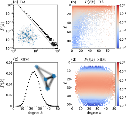
Figure 1: Degree distribution of a Barabási–Albert network and a stochastic block model. (a) The degree distribution of a Barabási–Albert network with 99,939 nodes. Each new node is connected to $m=2$ existing nodes (i.e., the degree of each node is at least 2) using preferential attachment. Then nodes with degrees larger than 100 [26] are removed from the network. The grey solid line is a guide-to-the-eye with slope -3 [27]. The inset shows a realization of a Barabási–Albert network with 100 nodes. Node size scales with their betweenness centrality. (b) The conditional probability $P(\ell|k)$ associated with the Barabási–Albert network generated in (a). (c) The degree distribution of a stochastic block model with four blocks and 100,000 nodes. The inset shows a realization of a stochastic block model with 800 nodes, but using the same block probability matrix. (d) The conditional probability $P(\ell|k)$ associated with the SBM. In both (b) and (d), all elements that are strictly zero are uncolored.

What remains is to assign network structures, extract $P(\ell|k)$ from them, and determine reasonable parameter values before calculating the optimal testing protocol $f_{k}(t)$. We apply our disease-control framework to (i) a Barabási-Albert (BA) network [28, 27] and (ii) a stochastic block model (SBM) [29] with four communities and probability matrix

$$P=10^{-4}\left(\begin{array}[]{llll}1&2&2&2\\ 2&4&2&2\\ 2&2&5&2\\ 2&2&2&3\end{array}\right).$$ (6)

These two network types exhibit properties, such as hub nodes with high degrees and community structure, that are observable in real-world contact networks [26, 30]. In the construction of the BA network, each new node is connected to 2 existing nodes. Figure 1(a) shows the degree distribution of a 99,939-node BA network that we use in this study. The conditional degree distribution $P(\ell|k)$ for a specific network can be directly evaluated as $E_{\ell,k}/(kN_{k})$ where $E_{\ell,k}$ is the number of edges connecting a node with degree $k$ with another node with degree $\ell$. A heatmap of the conditional degree distribution matrix of the BA network with the degree distribution $P(k)$ shown in (a) is given in Fig. 1(b). The degree distribution and the conditional degree distribution matrix of the 100,000-node SBM network are shown in Figs. 1(c) and (d), respectively. Taking into account empirical findings on the degree distributions in real-world contact networks [26], we use a degree cutoff of $k\leq K=100$.

Next, to constrain the parameter values, we first invoke estimates of the basic reproduction number (i.e., the average number of secondary cases that results from one case in a completely susceptible population), which for a network model is defined as [31]

$$\mathcal{R}_{0}=\rho(JV^{-1})$$ (7)

in which $\rho(\cdot)$ is largest eigenvalue (spectral radius), $V\equiv{\rm diag}(1/\gamma^{\rm u})\in\mathbb{R}^{K\times K}$ and $J\in\mathbb{R}^{K\times K}$ is the Jacobian of the linearized dynamical system (Eqs. (2) and (3)) about the disease-free state with $f_{k}=0$ corresponding to the initial, untested, and uncontrolled spread of the infection:

$$J_{ij}=iP(j|i)\frac{N_{i}}{N_{j}}\beta^{\text{u}},\quad i,j\leq K.$$ (8)

This “next generation” method associates $\mathcal{R}_{0}$ with the largest eigenvalue inherent to the dynamical system. Additional expressions for $\mathcal{R}_{0}$ for an uncorrelated degree network are given in Appendix A.

Empirically, the basic reproduction number for COVID-19 varies across different regions. For the early outbreak in Wuhan [32], $\mathcal{R}_{0}$ was estimated to be $3.49$, while for the early outbreak in Italy $\mathcal{R}_{0}\sim 2.43-3.10$ [33]. Here we set $\mathcal{R}_{0}=4.5$ which is suggested in [34] as the reproduction number of the COVID-19 in early spreading without intervention measures. To find the proper value of transmissibility, we adjusted $\beta^{\rm u}$ until Eq. (7) yields $\mathcal{R}_{0}(\beta^{\rm u})=4.5$. Our source codes are publicly available at https://gitlab.com/ComputationalScience/epidemic-control.

III Allocating limited testing resources

Without any testing constraints, it would be most effective for disease control to use a testing budget $f_{k}(t)$ sufficiently large to keep the fraction of untested individuals, $i_{k}^{\rm u}(t)$, close to zero. In general, the testing budgets are constrained by

$$f_{k}^{\min}\leq\frac{f_{k}(t)}{N_{k}}\leq f_{k}^{\max},$$ (9)

and the total testing rate is also bounded by availability and logistics of testing $\sum_{k=1}^{K}f_{k}(t)=F(t)$. The goal is to determine, under these constraints, the function $f_{k}(t)$ or $f_{k}(t)/N_{k}$ that most effectively reduces the total number of infections. In practice, high-degree nodes (highly social individuals) might be subject to more testing (and quarantining if positive) than low-degree nodes because of their higher expected rate of infecting others. This rationale would be translated as $f_{k}(t)/N_{k}>f_{k^{\prime}}(t)/N_{k^{\prime}}$ if $k>k^{\prime}$. In our numerical experiments, we use sufficiently broad bounds of $f_{k}(t)$ and set $f_{k}^{\min}=f_{\min}$ and $f_{k}^{\max}=f_{\max}$.

To minimize the number of total infections over time, we define a loss function as

$$L(T)=\int_{0}^{T}\!\!\mathrm{d}t\,\delta^{t}\!\sum_{k=1}^{K}ks_{k}(t)\!\sum_{\ell=1}^{K}\!{P(\ell|k)\over P(\ell)}\big{(}\beta^{\text{u}}i_{\ell}^{\text{u}}(t)+\beta^{*}i_{\ell}^{*}(t)\big{)},$$ (10)

where $\delta\in(0,1]$ denotes a discount factor, which describes how we balance between minimizing current infections and future infections. For example, medical resources can better handle patients and new treatments can be given time to develop if the number of infections are spread over longer time periods. These effects can be effectively incorporated in the loss function by using $\delta<1$. Minimizing the loss Eq. (10) is equivalent to minimizing the number of infections, weighted by the discount factor $\delta^{t}$, in the time horizon $[0,T]$.

The associated Hamiltonian is

$$H= \delta^{t}\sum_{k=1}^{K}ks_{k}(t)\sum_{\ell=1}^{K}\!{P(\ell|k)\over P(\ell)}\big{(}\beta^{\text{u}}i_{\ell}^{\text{u}}(t)+\beta^{*}i_{\ell}^{*}(t)\big{)}$$ (11)

$$\hskip 17.07164pt+\sum_{k=1}^{K}\left(\lambda^{s}_{k}\frac{\mbox{d}s_{k}(t)}{\mbox{d}t}+\lambda_{k}^{\text{u}}\frac{\mbox{d}i^{\rm u}_{k}(t)}{\mbox{d}t}+\lambda^{*}_{k}\frac{\mbox{d}i^{*}_{k}(t)}{\mbox{d}t}\right),$$

where $\lambda^{s}_{k}$, $\lambda^{\rm u}_{k}$, and $\lambda^{*}_{k}$ are adjoint variables associated with $s_{k}$, $i^{\rm u}_{k}$, and $i^{*}_{k}$, respectively. The dynamics for $(\lambda_{k}^{s},\lambda_{k}^{\rm u},\lambda_{k}^{*})$ obey

$$\frac{\mbox{d}\lambda_{k}^{s}}{\mbox{d}t}= \delta^{t}k\sum_{\ell=1}^{K}\!{P(\ell|k)\over P(\ell)}\big{(}\beta^{\text{u}}i_{\ell}^{\text{u}}(t)+\beta^{*}i_{\ell}^{*}(t)\big{)}$$

$$\quad-\lambda_{k}^{s}k\sum_{\ell=1}^{K}\!{P(\ell|k)\over P(\ell)}\big{(}\beta^{\text{u}}i_{\ell}^{\text{u}}(t)+\beta^{*}i_{\ell}^{*}(t)\big{)}$$ (12)

$$\quad+\lambda_{k}^{\rm u}k\sum_{\ell=1}^{K}\!{P(\ell|k)\over P(\ell)}\big{(}\beta^{\text{u}}i_{\ell}^{\text{u}}(t)+\beta^{*}i_{\ell}^{*}(t)\big{)},$$

$$\frac{\mbox{d}\lambda_{k}^{\text{u}}}{\mbox{d}t}= \frac{\beta^{\text{u}}}{P(k)}\sum_{j=1}^{K}P(k|j)s_{j}(t)(\delta^{t}-\lambda_{j}^{s}+\lambda_{j}^{\text{u}})$$ (13)

$$\qquad\qquad\qquad-\gamma^{\rm u}\lambda_{k}^{\rm u}-\frac{f_{k}(t)}{N_{k}}(\lambda_{k}^{\rm u}-\lambda_{k}^{*}),$$

$$\frac{\mbox{d}\lambda_{k}^{*}}{\mbox{d}t}= \frac{\beta^{*}}{P(k)}\sum_{j=1}^{K}\!P(k|j)s_{j}(t)(\delta^{t}-\lambda_{j}^{s}+\lambda_{j}^{\text{u}})-\gamma^{*}\lambda^{*}_{k}.$$ (14)

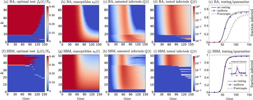
Figure 2: Optimal testing and quarantining strategy for the BA network using $T=200$ and discount factor $\delta=0.95$. (a) A heatmap of the PMP-optimal testing strategy (see Alg. 1) for the BA network. The corresponding populations of degree-$k$ susceptibles, untested infecteds, and tested infecteds are plotted in (b-d), respectively. (e) Time-evolution of the total fraction infected $1-\sum_{k=1}^{K}s_{k}(t)$ under the PMP-optimal testing strategy (dashed red). The fractions infected under hypothetical uniform testing (dashed blue/circle) and no testing (black) scenarios are shown for comparison. For the BA network, optimal testing both delays and suppresses epidemic spreading more effectively than uniform testing. The bottom row (f-j) shows analogous results for the SBM network. (f-i) shows the corresponding optimal testing rates, susceptible, untested infected, and untested infected populations with degree $k$ as a function of time. (j) shows the fraction infected as a function of time. Although optimal testing and quarantining reduces the fraction infected relative to uniform or no testing, its effects are only modestly better. The effects of optimal testing strategies are greater in the BA network because its distribution of node degrees are more heterogeneous and testing and quarantining high-degree nodes can more effectively control disease spread. On the other hand, since the node degree distribution in the SBM network is sharply peaked, an optimal testing strategy is less effective overall.

From the specific form

$$H= \sum_{k=1}^{K}(\delta^{t}-\lambda_{k}^{s}+\lambda_{k}^{\text{u}})k\sum_{\ell=1}^{K}\!{P(\ell|k)\over P(\ell)}\big{(}\beta^{\text{u}}i_{\ell}^{\text{u}}(t)+\beta^{*}i_{\ell}^{*}(t)\big{)}$$ (15)

$$\,\,+\sum_{k=1}^{K}\Big{[}f_{k}(t)(\lambda_{k}^{*}-\lambda_{k}^{\text{u}})i_{k}^{\text{u}}(t)-\gamma^{\text{u}}i_{k}^{\text{u}}(t)\lambda_{k}^{\text{u}}-\gamma^{*}i_{k}^{*}(t)\lambda_{k}^{*}\Big{]}$$

and the constraint of the total budget $\sum_{k=1}^{K}f_{k}(t)=F(t)$, using Pontryagin’s maximum principle, we calculate the optimal testing rates according to $(f_{k}^{*})=\mbox{argmin}_{f}H$. To minimize $H$, we have to minimize the term

$$\sum_{k=1}^{K}\frac{f_{k}(t)}{N_{k}}(\lambda_{k}^{*}-\lambda_{k}^{\text{u}})i_{k}^{\text{u}}(t).$$ (16)

Hence, we have to maximize those $f_{k}(t)$ with smallest coefficients $(\lambda_{k}^{*}-\lambda_{k}^{\text{u}})i_{k}^{\text{u}}(t)/N_{k}$ and minimize those $f_{k}(t)$ with largest coefficients, given the total budget constraint. In other words, we should give testing resources to those groups presumed to be at the highest risk, as quantified by the quantity $(\lambda_{k}^{*}-\lambda_{k}^{\text{u}})i_{k}^{\text{u}}(t)/N_{k}$.

We use the PMP-based testing algorithm outlined in Appendix B to iteratively calculate the optimal testing strategy and loss function (10). Numerical experiments for a BA and an SBM network were performed using a degree cutoff $K=100$ (see Sec. II). In accordance with empirical data on COVID-19 patients [35, 36, 37], we set $\gamma=\gamma^{\text{u}}=\gamma^{*}=(14)^{-1}/\text{day}$ and $\beta^{*}=\beta^{\text{u}}/10$. The transmissibility of untested individuals, $\beta^{\text{u}}$, is calculated according to Eq. (7) as $\beta^{\text{u}}=0.0417/\text{day}$ for the BA network and $\beta^{\text{u}}=0.0130/\text{day}$ for the SBM network. We set the discount factor $\delta=0.95$ so that initial infections contribute more to the loss function (10). The total daily number of SARS-CoV-2 tests in the US after an initial ramping-up phase in 2020 is about 0.6%/day [25]. Hence, we set

$$\sum_{k}f_{k}(t)=0.006N,$$ (17)

and $f_{\min}=0,f_{\max}=0.4N_{k}$. As initial condition, we use

$$~{}s_{k}(0)=P(k)-i_{k}^{\text{u}}(0), \,\,~{}i_{k}^{*}(0)=0,$$ (18)

$$i_{k}^{\text{u}}(0)=10^{-6}P(k), \,\,~{}r_{k}(0)=0,$$

corresponding to about 0.1 of an infected individual uniformly distributed on $N\approx 10^{5}$ susceptible nodes. The optimal testing strategy is supposed to identify those nodes that are most likely to be infected and transmit the disease to others. Upon using $T=200,\Delta{t}=0.1$ and $\delta=0.95$, we find the optimal testing strategy $f_{k}(t)/N_{k}$ for our BA network and plot it in Fig. 2(a). Here Eqs. (2)–(5) and (12)–(14) are solved using an improved Euler method. For the BA network, the value of the loss function defined in Eq. (10) is $L(T=200)=0.0114$ under the optimal testing strategy, while it is $L(T=200)=0.0330$ under uniform testing

$$f_{k}=F_{0}\frac{N_{k}}{N}.$$ (19)

Figs. 2(b-d) show the associated populations under optimal testing, while (e) shows the dynamics of the fraction of nodes infected, $1-\sum_{k=1}^{K}s_{k}(t)$, is significantly slowed relative to the no testing (black) and uniform testing (dashed blue/circle) cases. Fig. 2(f) plots the optimal testing rate for the SBM network. (g-i) show the corresponding subpopulations, and (j) plots the fraction of nodes infected under PMP-optimal, uniform, and no-testing conditions. For the SBM network, $L(T=200)=0.0564$ under the optimal strategy and $L(T=200)=0.0571$ under the uniform testing strategy, suggesting that the PMP approach yields better solutions than uniform testing. However, the improvement is modest and the SBM network is rather insensitive to testing and quarantining. The slight improvement from testing is shown by the reduction in the fraction infected relative to the no testing case (inset).

In both networks, nodes with larger degrees are more likely to be tested at the beginning of the outbreak [Figs. 2(a,f)], indicating that people with more contacts are more likely to infect others or get infected and should be given priority to get tested. Yet, in both networks, as time evolves, the optimal testing strategy tends to shift focus from higher degree nodes to nodes with smaller degrees because testing those nodes that were infected and have already recovered is not meaningful in terms of disease control.

Comparing Figs. 2(e) and (j), we see that the differences between optimal and uniform testing are larger for the BA network compared to the SBM. A possible explanation for this behavior is that in the BA network, the degree distribution $P(k)$ decays algebraically. Therefore, as long as testing focuses primarily on high-degree nodes, the spreading of the disease can be controlled very effectively since the majority of nodes have low degree and are more unlikely to be infected. On the other hand, for our SBM network, the degrees of most nodes are close to each other and larger than 10, indicating that nodes with a small degree are more likely to be infected compared to the BA network. Even if we use the same uniform testing rates [see Eq. (19)] in both networks, the proportion of infections in the BA network is less than that in the SBM network. Nodes with small degrees in the SBM are more likely to be infected than those in the BA network because they are more connected to other nodes.

IV Optimal vaccination policy

Optimal vaccination has also been studied within the classic SIR model [38]. However, devising vaccination strategies based on social network structure may provide a more refined and efficient way of administering vaccines and extinguishing an epidemic. Our simple testing model presented in the previous section can be straightforwardly adapted to describe vaccination on a network. The goal is to determine the optimal allocation of vaccine doses to a population with heterogeneous contacts to minimize the impact of the infection across the entire population.

For COVID-19, there are a variety of vaccines that require one or two shots [39]. In our simulations, we assume that the administered vaccine provides full protection after one shot and that a vaccinated individual will instantly leave the susceptible group and enter the recovered group. This means that vaccinated individuals will no longer be infectious and can be treated as “recovered” after receiving one vaccination dose. Other mechanisms such as prime-boost protocols and time delays between vaccination and onset of immune response can also be accounted for in similar models as detailed in [40].

We reformulate Eqs. (2)-(5) to study optimal vaccination protocols that are constrained by vaccine supplies in a heterogeneous population. For simplicity, we do not take into account the effect of testing and quarantining when devising optimal vaccinating strategies, although testing and vaccination can be performed concurrently. The resulting rate equations are

$$\frac{\mbox{d}s_{k}(t)}{\mbox{d}t} =-\beta ks_{k}(t)\sum_{\ell=1}^{K}\!\frac{P(\ell|k)}{P(\ell)}i_{\ell}(t)-\frac{v_{k}(t)}{N},$$ (20)

$$\frac{\mbox{d}i_{k}(t)}{\mbox{d}t} =\beta ks_{k}(t)\sum_{\ell=1}^{K}\!\frac{P(\ell|k)}{P(\ell)}i_{\ell}(t)-\gamma i_{k}(t),$$ (21)

$$\frac{\mbox{d}r_{k}(t)}{\mbox{d}t} =\gamma i_{k}(t)+\frac{v_{k}(t)}{N},$$ (22)

where $v_{k}(t)$ is the rate of vaccination of susceptibles with degree $k$ at time $t$. Once vaccinated, susceptibles become “recovered” because they are immunized and no longer susceptible to the infection. The total rate of administering vaccines at time $t$ is defined as

$$\sum_{k=1}^{K}v_{k}(t)=V(t).$$ (23)

In other words, in time increment $\Delta t$ at time $t$, we can administer only $V(t)\Delta t$ doses. Eq. (20) assumes that vaccination is resource-limited and that the rate of protecting susceptibles is proportional only to the rate $v_{k}(t)$ of administering vaccines. In addition, we assume that the vaccination rate for different subpopulations is confined to the interval

$$v_{\min}\leq\frac{v_{k}(t)}{Ns_{k}(t)}\leq v_{\max},$$ (24)

where $v_{\min},v_{\max}\in[0,1]/\textrm{day}$ are minimum and maximum vaccination rates. Note that vaccines are allocated only to susceptibles, while tests are typically given to individuals of all categories: susceptible, infected, and recovered, according to their relative proportions. To formulate the vaccine distribution problem in a heterogeneous contact network, we use the following loss function

$$L(T)=\int_{0}^{T}\!\mathrm{d}t\,\delta^{t}\sum_{k=1}^{K}ks_{k}(t)\sum_{\ell=1}^{K}\!{P(\ell|k)\over P(\ell)}\beta(t)i_{\ell}(t),$$ (25)

with the aim of minimizing the total number of infections over time (with a constant discount factor $\delta\in(0,1]$) by appropriately distributing vaccines to groups with different degree $k$ at different rates.

Figure 3: Optimized vaccination model. (a) Heatmap of the optimal vaccination strategy $v_{k}(t)/(s_{k}(t)N_{k})$ for the BA network given by Alg. 1. (b,c) show the corresponding susceptible and infected subpopulations $s_{k}(t)$ and $i_{k}(t)$, while (d) plots the fraction infected as a function of time, derived from solving Eqs. (20)–(22) under optimal vaccination using a discount factor $\delta=0.95$. The dashed red curve indicates the fraction infected under optimal vaccination. For comparison, the infected population under no vaccination (solid black) and constant, uniform (dashed blue/circles) vaccination are also plotted and show how optimizing vaccination significantly suppresses infectivity. (e-h) show the corresponding quantities for the SBM network. Optimal vaccination is less effective at decreasing infection in the SBM network than in the BA network, again because of the SBM’s peaked (more homogeneous) node degree distribution. Note from the logarithmic scale that vaccination is qualitatively more effective in reducing infections than testing and quarantining.

To minimize the loss function (25), we construct the Hamiltonian

$$H= \beta\delta^{t}\sum_{k=1}^{K}ks_{k}(t)\sum_{\ell=1}^{K}{P(\ell|k)\over P(\ell)}i_{\ell}(t)$$ (26)

$$\qquad\qquad\qquad+\sum_{k=1}^{K}\Big{(}\lambda^{s}_{k}\frac{\mbox{d}s_{k}(t)}{\mbox{d}t}+\lambda_{k}^{i}\frac{\mbox{d}i_{k}(t)}{\mbox{d}t}\Big{)},$$

$$\>= \beta\sum_{k=1}^{K}(\delta^{t}-\lambda_{k}^{s}+\lambda_{k}^{i})ks_{k}(t)\sum_{\ell=1}^{K}\!{P(\ell|k)\over P(\ell)}i_{\ell}(t)$$

$$\qquad\qquad\qquad+\sum_{k=1}^{K}\Big{(}\frac{v_{k}(t)}{N}\lambda_{k}^{s}(t)-\gamma i_{k}(t)\Big{)}$$

where $\lambda_{k}^{s}$ and $\lambda_{k}^{i}$ are the Lagrange multipliers satisfying the differential equations

$$\frac{\mbox{d}\lambda_{k}^{s}}{\mbox{d}t}= \beta k\sum_{\ell=1}^{K}{P(\ell|k)\over P(\ell)}i_{\ell}(t)(\delta^{t}-\lambda_{k}^{s}+\lambda_{k}^{i})$$ (27)

$$\frac{\mbox{d}\lambda_{k}^{i}}{\mbox{d}t}= \frac{\beta}{P(k)}\sum_{j=1}^{K}P(k|j)js_{\ell}(t)(\delta^{t}-\lambda_{j}^{s}+\lambda_{j}^{i})-\gamma\lambda_{k}^{s}.$$ (28)

Therefore, minimizing the loss function (25) for the given dynamics is equivalent to minimizing the Hamiltonian (26) using Pontryagin’s maximum principle. From the constraints (23) and (24), minimizing the Hamiltonian is achieved by giving vaccination $v_{k}$ to those subpopulations with the smallest $\lambda_{k}^{s}$. We can still use Alg. 1 to solve the minimization problem (25) numerically and obtain the optimal strategy.

In the US, about two million doses of SARS-CoV-2 vaccines were delivered in May 2021 [41], most of which were two-dose vaccines. Since approximately $0.3\%$ of the entire US population is fully vaccinated daily, we set $V(t)=0.003N/\text{day}$, $v_{\min}=0/\text{day}$, and $v_{\max}=0.4/\text{day}$ in the constraint (24). The infection rates $\beta$ are set to be $0.0417/\text{day}$ for the BA network and $0.0130/\text{day}$ for the SBM network, and the recovery rate $\gamma=(14)^{-1}/\text{day}$. For comparison, we also simulate a vaccination strategy with a uniform vaccination rate

$$v_{k}(t)=\frac{s_{k}(t)V(t)}{\sum_{k=1}^{K}s_{k}(t)}.$$ (29)

In all simulations, we use the following initial condition:

$$i_{k}(0)=10^{-6}P(k),~{}r_{k}(0)=0,s_{k}(0)=P(k)-i_{k}(0).$$ (30)

We plot the PMP-optimal vaccination strategy $v_{k}/N_{k}$ in Figure 3(a) and the corresponding susceptible and infected $k$-degree subpopulations $s_{k}(t)$ and $i_{k}(t)$ in (b) and (c). We set $T=150,\Delta{t}=0.1$ and we use an improved Euler method to numerically solve Eqs. (20)–(22), (27)–(28). Alg. 1 is applied (without the infected and tested compartment) to determine the optimal vaccination strategy by the PMP approach. For the BA network, $L(T=150)=1.241\times 10^{-5}$ under the PMP-optimal strategy and $L(T=150)=0.01990$ under a uniform vaccination rate. Figure 3(d) shows that the optimal vaccination strategy on a BA network significantly reduces the fraction infected compared to the uniform vaccination strategy. (e-h) show the corresponding quantities for the SBM network for which $L(T=150)=0.0211$ under the optimal vaccination strategy and $L(T=150)=0.0360$ under a constant, uniform vaccination strategy. In both networks, the optimal vaccination strategies obtained via Alg. 1 tend to prioritize those nodes with higher degrees first and eventually expand to those nodes with smaller degrees [see Figs. 3(a) and (e)]. As with testing and quarantining, the reduction in the fraction infected by vaccination is greater in the BA network. Since the BA network has a degree distribution with algebraic decay, the effect of the optimal vaccination strategy will be more pronounced than for the SBM, whose nodes have similar degrees.

V Discussion and Conclusions

Effective testing and vaccination strategies are an essential part of epidemic management. In this paper, we derived optimal testing and vaccination policies by applying Pontryagin’s maximum principle to a degree-based epidemic model in a heterogeneous contact network. We complemented our analytical results with reinforcement learning (RL) approaches that identify effective policies. (see Appendix C)

Figure 4: Total fraction infected under testing or vaccination model as a function of different intervention starting times $t_{0}$. We minimize the corresponding loss function at $T=150$ and use $\delta=0.95$. (a) The fraction infected in the BA network as a function of start times using different testing amplitudes $F$. At larger $F$, there is a decrease in infected population for later starts of testing at early times. This nonmonotonic response arises from $\delta<1$ that weights early infections more strongly in the loss function, which remains monotonic in $t_{0}$ under optimization as shown in (b). The effect of delayed vaccination on the fraction infected is shown in (c), with the corresponding loss function shown in (d). For the SBM network, the fraction infected as a function of testing start time shown in (e) reflects the small effect of testing on the infected population. Both the fraction infected and loss function (f) are monotonic in starting time. The starting time dependence of the fraction infected on an optimally vaccinated SBM network in (g) shows a monotonic and smooth decrease in effectiveness as vaccination is delayed. In (h), the loss function for vaccination on the SBM network also monotonically increases with start time.

Our analytical results show that optimal testing and vaccination policies under resource constraints initially tend to prioritize nodes with higher degrees to control spread of the disease. In situations where the number of contacts of individuals is known or can be estimated with reasonable precision, Algs. 1 and 2 may be useful to identify effective epidemic management strategies. Using our control-theoretic approach, we also explored the relative effectiveness of testing and vaccination under different conditions.

V-A Effects of delayed intervention

First, we consider the effectiveness of interventions as a function of the time between the first infection and the implementation of testing or vaccination. The initial conditions are set to be the same as Eqs. (18) and (30). Fig. 4 shows the total fraction infected and the loss functions at $T=150$, for both the BA and SBM networks, as a function of intervention starting time $t_{0}$. We set $F=F(t)\mathds{I}_{t>t_{0}}$ or $V=V(t)\mathds{I}_{t>t_{0}}$ and explore the effects of different constant levels of test kits or vaccine availability, $F(t)=0.002,0.004,0.006,0.008N/\text{day}$ and $V(t)=0.001,0.002,0.003,0.004N/\text{day}$, respectively. The transmissibility rates $\beta^{\text{u}},\beta^{*},\beta$ and the recovery rates $\gamma^{\text{u}},\gamma^{*},\gamma$ are set to the same values as those used in Section III for the testing model and those used in Section IV for the vaccination model.

At higher levels of $F$ and $V$, the high-$k$ nodes are addressed sooner and total infections can be reduced. For the vaccination model applied to both networks, an earlier intervention time will always lead to fewer infected nodes. In the BA network, there exists an overall vaccination-rate-dependent starting time before which disease spread can be totally suppressed. Overall, we found that earlier and stronger intervention measures lead to more effective control of the spreading of the disease and a smaller loss function defined in Eqs. (10), (25).

However, for $\delta<1$ ($\delta=0.95$ in this study), we found that the final infected proportions can actually decrease with later testing starting times $t_{0}$ shortly after the initial infection, particularly with larger $F$. The testing loss function monotonically increases with $t_{0}$, a feature that is not preserved in the total final infection ratio. This qualitative difference can arise when $\delta<1$ because the strategy of earlier testing tends to minimize initial infections in a way that reduces the loss function, even though the corresponding infection levels may be even larger than those associated with later starts in testing.

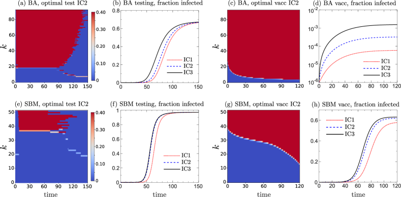
Figure 5: Dependence of intervention effectiveness on the degree of the initial infected individual. (a) The PMP-optimal testing strategy computed using IC2 ($k_{\rm i}=20$) on the BA network. Strategies for IC1 ($k_{\rm i}=3$) and IC3 ($k_{\rm i}=90$) are qualitatively similar (not shown) with small differences at the beginning leading to the different delays in the infection dynamics shown in (b). Specifically, for IC1 and IC3 the initial transient of the optimal testing strategy maximizes the testing rate for the subpopulation with the same degree as $k_{1}$ and $k_{3}$, respectively, indicating that the optimal testing strategy is sensitive to the degree properties initial seed infection. Once the disease spreads out, the testing strategies “forget” the initial condition and converge to each other. Despite optimal testing, initial infecteds with higher degree, such as IC3, lead to earlier spread of the epidemic. Results are found by using a discount factor $\delta=0.95$, the optimal strategy given in Alg. 1, and solving Eqs. (2)–(5). (c-d) The optimal vaccination strategy for IC2 and the associated fraction infected for the BA network. As with testing, the vaccination strategies associated with IC1 ($k_{\rm i}=5$) and IC3 ($k_{\rm i}=30$) lead to differences in infection magnitudes. However, the optimal vaccination strategies are insensitive to different initial conditions, even at early times. Since the mechanism of vaccination is always to protect high-degree susceptibles, the vaccination strategies are not as dependent on the current infected population as the testing strategies are. (e) shows the optimal testing strategy for the SBM network, assuming IC2 ($k_{\rm i}=20$). (f) The fraction infected exhibits slower dynamics for smaller-degree initial conditions. (g) Optimal vaccination strategy for IC2 in the SBM network and (h), the associated infected fraction showing both delay and amplitude changes with changes in the initial condition.

V-B Dependence on initial conditions

Besides the start time of testing or vaccination, initial conditions may also affect the optimal strategy. For example, the initial propagation of the disease may depend on the degree $k$ of the first infected individual [42]. Instead of an initial infectious source who is uniformly distributed across all nodes, as described in Eqs. (18) and (30), we vary the degree of the first infected node and explore how the strategies change as a function of concentrated initial condition $i_{k}(0)=N_{0}\delta_{k,k_{\rm i}}/N$. We take $N_{0}=10^{-6}N$ for both networks, $k_{\rm i}=3,20,90$ for the BA network, and $k_{\rm i}=5,20,30$ for the SBM network. These different initial conditions are denoted IC1, IC2, and IC3 for each network, respectively.

Fig. 5 shows that under optimal testing and vaccination, a smaller degree of the first infected source typically leads to a smaller subsequent infected population. Optimal testing strategies are seen to be visibly dependent on the initial conditions, i.e., the degree of the initial infected patient. This sensitivity arises because testing those who are not infected will only waste testing resources. After early stage spread of the disease, the testing strategy becomes insensitive initial condition because persons with all degrees are infected and those with a higher degree tend to be infected sooner.

The optimal vaccination strategies obtained through Alg. 1 are also relatively insensitive to initial conditions in both networks, particularly at at longer times. Although not shown, the optimal strategies associated with different ICs are mostly the same times because nodes with larger degrees tend to always be vaccinated first to minimize the loss function Eq. (25). Susceptibles with higher degrees are more vulnerable and should be vaccinated first to mitigate subsequent infection events. The strategy differences disappear at later times.

If more information on contact patterns of individual nodes is available, it is possible to further refine the proposed policies using interventions that rely not only on node degrees, but also on other structural features such as percolation and betweenness centrality [15, 43].

In addition to the application of control-theoretic methods, we also utilized reinforcement learning (RL) to identify effective testing and vaccination strategies. On occasions when the best optimal strategy can be analytically solved, the controls derived from the Pontryagin’s maximum principle outperform RL-based interventions; yet reinforcement learning is applicable to epidemic management problems when analytic solutions are not available. Our results also indicate that optimal-control theory may be helpful for pre-training and restricting the space of possible actions, which may lead to more efficient RL algorithms.

Further generalizations of the derived optimal testing and vaccination strategies include devising different loss functions other than Eqs. (10) and (25) to take into account factors such as economic effects and prioritizing certain demographics groups (e.g., individuals with comorbidities). Furthermore, another possible direction for future research is to devise optimal testing and vaccination resource allocation strategies under disease-induced resource constraints [44]. Instead of using RL-based control strategies, it is also a worthwhile direction for future research to apply neural ODE control frameworks [45, 46] to the studied resource allocation problems since these control methods showed a better performance than reinforcement learning and numerical adjoint system solvers. Finally, in addition to obtaining and even combining testing and/or vaccination strategies, our results indicate that different network structures (e.g., BA vs. SBM) have different susceptibilities to optimal strategies. Thus, policies such as selective social distances can potentially be used to shift network structure towards one that is more sensitive to direct testing and vaccination strategies.

Appendix A Basic reproduction number

In this appendix, we analytically derive the basic reproduction number $\mathcal{R}_{0}$ for uncorrelated networks and compare the resulting values with those obtained using Eqs. (7) and (8). As a starting point, we note that the conditional degree distribution $P(\ell|k)$ can be expressed in terms of a symmetric (for undirected networks) joint degree distribution $P(\ell,k)$, the probability that a randomly chosen edge connects two nodes with degrees $\ell$ and $k$. Marginalizing $P(\ell,k)$ over $\ell$ yields the distribution over edge ends [47] $P_{\rm e}(\ell)\equiv\sum_{k}P(\ell,k)=\ell P(\ell)/\langle k\rangle$, where $\langle k\rangle=\sum_{k}kP(k)$ is the mean degree. The conditional degree distribution is related to the joint distribution via

$$P(\ell|k)=\frac{P(\ell,k)}{P_{\rm e}(k)}=\frac{\langle k\rangle P(\ell,k)}{kP(k)},$$ (31)

which can be further simplified in the uncorrelated network limit where $P(\ell,k)\approx P_{\rm e}(k)P_{\rm e}(\ell)$:

$$P(\ell|k)\approx\frac{\ell P(\ell)}{\langle k\rangle}.$$ (32)

Eqs. (31) or (32) can be used as a simpler replacement for $P(\ell|k)$ in Eqs. (2) and (3) if $E_{\ell,k}/(kN_{k})$ is not directly accessible. For example, for an uncorrelated network (i.e., for $P(\ell|k)=\ell P(\ell)/\langle k\rangle$), we find

$$\frac{\mbox{d}i^{\rm u}_{k}(t)}{\mbox{d}t}=\beta^{\rm u}\frac{ks_{k}(t)}{\langle k\rangle}\sum_{\ell}\ell i^{\rm u}_{\ell}(t)-\gamma^{\rm u}i^{\rm u}_{k}(t),$$ (33)

where we have set testing rates $f_{k}(0)=0$ at the start of the infection. According to [22], we define

$$I^{\rm u}(t)\coloneqq\sum_{k}i_{k}^{\rm u}(t),\,\,\,J^{\rm u}(t)\coloneqq\sum_{k}ki_{k}^{\rm u}(t)$$ (34)

and obtain

$$\dot{I}^{\rm u}(t) =\beta^{\rm u}J^{\rm u}(t)-\gamma^{\rm u}I^{\rm u}(t),$$ (35)

$$\dot{J}^{\rm u}(t) =\beta^{\rm u}\frac{\langle k^{2}\rangle}{\langle k\rangle}J(t)-\gamma^{\rm u}J^{\rm u}(t).$$

We perform a linear stability analysis around the disease-free state $(I^{*},J^{*})=(0,0)$ and find the eigenvalues to Eqs. (35):

$$\lambda_{\pm}=-\gamma^{\rm u}\pm\beta^{\rm u}\frac{\langle k^{2}\rangle}{\langle k\rangle}.$$ (36)

The transition from negative to positive eigenvalues occurs for $-\gamma^{\rm u}+\beta^{\rm u}\langle k^{2}\rangle/\langle k\rangle=0$. Hence, the basic reproduction number is

$$\mathcal{R}_{0}=\frac{\beta^{\rm u}}{\gamma^{\rm u}}\frac{\langle k^{2}\rangle}{\langle k\rangle}=\frac{\beta^{\rm u}}{\gamma^{\rm u}}\left(\langle k\rangle+\frac{{\rm{Var}}[k^{2}]}{\langle k\rangle}\right).$$ (37)

If we use the conditional degree distribution $P(\ell|k)=(\ell-1)P(\ell)/\langle k\rangle$ proposed by Kiss et al. [22] to account for a reduction in neighboring susceptible vertices, the corresponding basic reproduction number is modified to

$$\mathcal{R}_{0}^{\rm Kiss}=\frac{\beta^{\rm u}}{\gamma^{\rm u}}\left(\langle k\rangle-1+\frac{{\rm{Var}}[k^{2}]}{\langle k\rangle}\right).$$ (38)

The mean degrees of the BA and SBM networks are 3.77 and 23.14, and the variances for the BA and SBM networks are 20.40 and 36.62, respectively. Using the values $\gamma^{\rm u}=14^{-1}/{\rm day}$ and $\beta^{\rm u}=0.0417/\text{day}$ for the BA network, we find that the basic reproduction numbers $\mathcal{R}_{0}=5.361$ and $\mathcal{R}_{0}^{\rm Kiss}=4.777$ are larger than 4.5, the value we used to determine $\beta^{\rm u}$ according to the next-generation matrix method (Eqs. (7) and (8)). The observed approximation errors in Eqs. (37) and (38) are a consequence of the assumption that the underlying network is uncorrelated. For the SBM network, we find $\mathcal{R}_{0}=4.499$ and $\mathcal{R}_{0}^{\rm Kiss}=4.317$, close to the 4.5 value used to find $\beta^{\rm u}=0.0130$ using Eqs. (7) and (8).

To summarize, our comparison shows that in the SBM model where the degrees of neighbors are uncorrelated, Eqs. (37) and (38) give close approximations of the actual reproduction number calculated from the next-generation matrix method (7). For the BA network, degree correlations make Eqs. (37) and (38) overestimate the actual reproduction number. Therefore, we recommend using the next-generation matrix method to numerically determine the basic reproduction number unless degree correlations are weak and Eqs. (37) and (38) can provide accurate estimates of $\mathcal{R}_{0}$.

Appendix B Optimal testing and vaccination algorithms

Below, we explicitly give the pseudo-code for the testing and quarantine model based on Pontryagin’s maximum principle.

Algorithm 1 Pseudo-code for determining optimal testing strategies based on Pontryagin’s maximum principle.

1:Initialize $t=0$, $s_{k}(0),i^{\text{u}}_{k}(0),i^{*}_{k}(0)$, $\Delta t$, $T=n\Delta{t}$, $\beta^{\text{u}},\beta^{*}$, $\gamma^{\text{u}},\gamma^{*}$, $\delta$, initial strategy $F(k\Delta{t}),k$, $f_{\max}$, $f_{\min}$, $\epsilon$, $iter_{\max}$

2:for $k=0:n-1$ do

3:     Calculate $s_{k}(t),i_{k}^{*}(t),i_{k}^{\text{u}}(t)$ under the strategy $F(k\Delta{t})$ from Eqs. (2)–(4)

4:end for

5:Set $\lambda_{k}^{s},\lambda_{k}^{\text{u}},\lambda_{k}^{*}=0,k=n$

6:Calculate the loss function $L_{1}$ in Eq. (10)

7:for $k=n-1:0$ do

8:     Calculate $\lambda_{k}^{s},\lambda_{k}^{\text{u}},\lambda_{k}^{*}$ under the strategy $F(k\Delta{t})$ from Eqs. (12)–(14)

9:end for

10:for $k=0:n-1$ do

11:     First renew the strategy $F(k\Delta{t})$, then calculate $s_{k},i_{k}^{\text{u}},i_{k}^{*}$ under the strategy $F(k\Delta{t})$ from Eqs. (2)–(4)

12:end for

13:Calculate the loss function $L_{2}$ in Eq. (10)

14:$i\leftarrow 1$

15:while $|L_{1}-L_{2}|>\epsilon~{}\&\&~{}i<iter_{\max}$ do

16:     $i\leftarrow i+1$

17:     $L_{1}\leftarrow L_{2}$

18:     Set $k=n,\lambda_{k}^{s},\lambda_{k}^{\text{u}},\lambda_{k}^{*}=0$

19:     for $k=n-1:0$ do

20:         Calculate $\lambda_{k}^{s},\lambda_{k}^{\text{u}},\lambda_{k}^{*}$ under the strategy $F(k\Delta{t})$ from Eqs. (12)–(14)

21:     end for

22:     for $k=0:n-1$ do

23:         First renew the strategy $F(k\Delta{t})$, then calculate $s_{k},i_{k}^{\text{u}},i_{k}^{*}$ under the strategy $F(k\Delta{t})$ from Eqs. (2)–(4)

24:     end for

25:     Calculate the Loss function $L_{2}$ in Eq. (10)

26:end while

Appendix C Reinforcement-learning strategy

To identify effective testing and vaccination strategies, we also investigated reinforcement-learning (RL) approaches. RL explores the space of all possible actions and directly optimizes the loss functions for testing and vaccination defined in Eqs. (10) and (25). Here, we use an RL approach with experience replay to learn both the optimal testing strategy in Eqs. (2)–(5) and the optimal vaccination strategy in Eqs. (20)–(22).

Typically, applying a policy-gradient method to a continuous action space will usually yield poor results due to the inability of such methods to explore the whole space. However, using our previous results based on Pontryagin’s maximum principle (PMP), we know that the optimal strategy is always obtained by maximizing the testing and vaccination rates for subpopulations presumed to be at a higher risk.

Therefore, we do not need to explore the whole space of all possible actions. Instead, from Eqs. (16), (26), we can restrict our strategy space to the extreme points of the set

$$\{(f_{k})|_{k=1}^{K}|\sum_{k=1}^{K}f_{k}=F(t),f_{\min}\leq\frac{f_{k}}{N_{k}}\leq f_{\max}\}$$ (39)

for determining testing-resource allocation and the extreme points of the set

$$\{(v_{k})|_{k=1}^{K}|\sum_{k=1}^{K}v_{k}=V(t),v_{\min}\leq\frac{v_{k}}{Ns_{k}(t)}\leq v_{\max}\}$$ (40)

for determining vaccination-resource allocation at each step. The set of extreme points represents all strategies that maximize the testing/vaccination rates for some groups and minimize them for other groups. Such strategies also cannot be written as nontrivial convex combinations of other strategies. By confining ourselves to extreme points, the possible action space is reduced to a finite set on which we perform RL.

Since the curse of dimensionality increases the number of all possible strategies exponentially with $K$, we further restrict our RL approach to networks with degree cutoff $K=20$. This additional constraint allows us to perform RL with a computation time of about 30 days for the testing model on the BA network, 3 days for the testing model on the SBM network, 6 hours for the vaccination model on the BA network, and 2 hours for the vaccination model on an SBM network. All computations are performed using Python 3.8.10 on a laptop with a 4-core Intel(R) Core(TM) i7-8550U CPU @ 1.80 GHz.

Algorithm 2 Pseudo-code of Q-Learning in testing resource allocation.

1:Initialize $F,\delta,C$, $i^{u}_{k}(0),i^{*}_{k}(0),\beta^{u},\beta^{*},\gamma^{u},\gamma^{*},M,\epsilon$

2:Initialize replay memory $D$

3:Randomly initialize the hyperparameter $\Theta=\Theta^{-}$ for evaluating the action value function $Q^{*}(\mathcal{S},\mathcal{A};\Theta)$

4:for episode $\ell=1:M$ do

5:     Initialize $\mathcal{S}_{0}$

6:     for $t=0:T_{\text{max}}-1$  do

7:         With probability $\epsilon$, randomly select an action $a_{i}$

8:         otherwise select $\mathcal{A}_{t}=\mbox{argmax}_{\mathcal{A}}Q(\mathcal{S}_{t},\mathcal{A};\Theta)$

9:         Execute action $\mathcal{A}_{t}$ and observe reward $R_{t}$ and state $\mathcal{S}_{t+1}$

10:         Store transition $(\mathcal{S}_{t},\mathcal{A}_{t},R_{t},\mathcal{S}_{t+1})$ in $D$

11:         Sample random minibatch of transitions $(\mathcal{S}_{j},\mathcal{A}_{j},R_{j},\mathcal{S}_{j+1})$ from $D$

12:         if $j=T_{\text{max}}-1$  then

13:              Set $y_{j}=R_{j}$

14:         else

15:              Set $y_{j}=R_{j}+\delta\max_{\mathcal{A}^{\prime}}\hat{Q}(\mathcal{S}_{j+1},\mathcal{A}^{\prime};\Theta^{-})$

16:              Perform a gradient descent step on the minibatch $\sum_{j}[y_{j}-Q(\mathcal{S}_{j},\mathcal{A}_{j};\Theta)]^{2}$ with respect to the network parameter $\Theta$

17:         end if

18:     end for

19:     Every $C$ steps reset $\Theta^{-}=\Theta$

20:end for

To identify effective testing and vaccination strategies, we use the reward functions (10) and (25). We define the reward at time $t_{i}=i\Delta{t}$ as

$$R(\mathcal{S}_{i},\mathcal{A}_{i},i)=\sum_{k=1}^{K}\left[s_{k}(t_{i+1})-s_{k}(t_{i})\right],$$ (41)

the “negative” of the number of total infections during the time period $[t_{i},t_{i+1})$. Here, the state $\mathcal{S}_{i}$ and action $\mathcal{A}_{i}$ are

$$\mathcal{S}_{i}= (s_{1}(t_{i}),\dots,s_{K}(t_{i}),i^{\text{u}}_{1}(t_{i}),\dots,i^{\text{u}}_{K}(t_{i}),$$ (42)

$$\qquad\qquad i^{*}_{1}(t_{i}),\dots,i^{*}_{K}(t_{i}))\in(\mathbb{R})^{3K},$$

$$\mathcal{A}_{i}= (f_{1}(t_{i}),\dots,f_{K}(t_{i}))\in(\mathbb{R})^{K}$$

for the testing model Eqs. (2)–(5) and

$$\mathcal{S}_{i} =(s_{1}(t_{i}),\dots,s_{K}(t_{i}),i_{1}(t_{i}),\dots,i_{K}(t_{i}))\in(\mathbb{R})^{2K},$$ (43)

$$\mathcal{A}_{i} =(v_{1}(t_{i}),\dots,v_{K}(t_{i}))\in(\mathbb{R})^{K}$$

for the vaccination model Eqs. (20)–(22). We recursively define the state-value function under a certain policy $\pi$ to be

$$V^{\pi}(\mathcal{S}_{i},i)=\begin{cases}V^{\pi}(\mathcal{S}_{i+1})\delta+R(\mathcal{S}_{i},\pi(\mathcal{S}_{i})),&t_{i}<T_{\text{max}},\\ 0,&t_{i}=T_{\text{max}},\\ \end{cases}$$ (44)

where $\pi(\mathcal{S}_{i})$ is the action determined under policy $\pi$ given $\mathcal{S}_{i}$ and $\delta\in(0,1]$ is a discount factor. We also define the action-value function to be

$$Q^{\pi}(\mathcal{S}_{i},\mathcal{A}_{i},i)=\begin{cases}V^{\pi}(\mathcal{S}_{i+1})\delta+R(\mathcal{S}_{i},\mathcal{A}_{i},i),&t_{i}<T_{\text{max}}-1,\\ R(\mathcal{S}_{i},\mathcal{A}_{i},i),&t_{i}=T_{\text{max}}-1.\\ \end{cases}$$ (45)

We use $Q^{*}$ and $V^{*}$ to denote the action-value and state-value functions, respectively, under the best policy and apply the deep Q-learning algorithm, which has been used to find the optimal strategy [48].

Here, we use a neural network with a hyperparameter set $\Theta$, representing neural-network weights to estimate the action-value function under the best policy $Q^{*}(\mathcal{S},\mathcal{A};\Theta)$, which is improved over epochs by Alg. 2. We use another neural network with hyperparameter set $\Theta^{-}$ updated every $C=4$ steps to match $\Theta$. An illustration of the two neural networks, their layers, and activation functions is shown in Fig. 6.

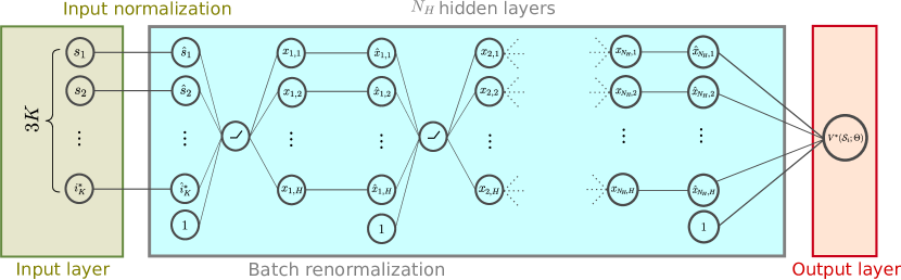
Figure 6: Illustration of the neural network used to identify effective testing and vaccination strategies. The inputs of the input layer are $(s_{k}(t);i^{\text{u}}_{k}(t);i^{*}_{k}(t))\in\mathbb{R}^{3K}$. For each hidden layer $i$ ($1\leq i\leq N_{H}$), we normalize the corresponding outputs $x_{i,j}$ for all samples in a minibatch such that the resulting values $\hat{x}_{i,j}$ have zero mean and unit variance. These values are used as inputs to a rectified linear unit (ReLU) activation function in the next hidden layer. Neurons labeled 1 are bias terms. The output $V^{*}(S_{i};\Theta)$ is an estimate of the state-value function under the optimal policy (see Eq. (44)), where $\Theta$ denotes the set of hyperparameters.

We use a neural network with $N_{H}=4$ hidden layers $H=30$ neurons in each layer. The input data is the state at the $i^{\text{th}}$ step $\mathcal{S}_{i}$, and the output is $V^{*}(\mathcal{S}_{i};\Theta)$, the prediction for the optimal state-value function generated by the neural network. In each layer, the batch normalization technique is used before a rectified linear unit (ReLU) function is applied as an activation function. We compare the optimal strategies based on the PMP approach from Alg. 1 with Alg. 2. We set $T=100$ and $\Delta{t}=1$ so that the strategy is updated every day. Here, we use $f_{\min}=0.002/\text{day},f_{\max}=0.4/\text{day}$. We used Eq. (7) with $\gamma^{\text{u}}=(14)^{-1}/\text{day}$ to calculate $\beta^{\text{u}}=0.0703/\text{day}$ for the $K=20$ BA network and $\beta^{\text{u}}=0.0632/\text{day}$ for the $K=20$ SBM network. Both optimal strategies are also compared to the uniform vaccination strategy (29). For RL, we train the underlying neural network for $M=100$ epochs using Alg. 2.

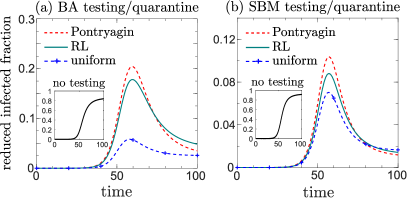
Figure 7: Reduction in fractions of infected individuals calculated as the difference between the fractions infected obtained with testing and without testing for the BA network shown in (a) and the SBM network shown in (b). The optimal control approach based on PMP reduces early infections the most. RL outperforms uniform testing in reducing the number of early-stage infections. Additionally, the effect of the optimal strategy is more striking in the BA network because it has a more heterogeneous node degree distribution.

Figure 7 shows the differences between the infected fractions in simulations with and without testing. The PMP-based optimal control reduces early infections the most for both BA and SBM networks. Early infections contribute more to the loss function (10) since we set the discount factor to $\delta=0.95$. We also observe that RL-based testing strategies outperform uniform testing in reducing early-stage infections. Comparing Fig. 7(a,b), the effect of the optimal vaccination strategy in the BA network is more pronounced than that in the SBM network. In the BA network, node degrees are more heterogeneous and most nodes have small degrees, indicating that epidemic spreading can be controlled effectively as long as the few high-degree nodes are monitored and tested. Finally, comparing the result of the optimal-control approach in Fig. 7 with Fig. 2, we observe that with a smaller $K$ in the SBM network, the effect of the optimal vaccination strategy is less apparent because node degrees are more homogeneous.

Next, we compared the PMP approach with the RL approach for the optimal vaccination strategy model Eqs. (20)–(22). Here, we set $v_{\min}=0.0001,v_{\max}=1$.

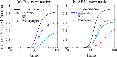
Figure 8: Reduction in fractions of infected individuals calculated as the difference between the fractions infected obtained with vaccination and without vaccination for the BA network shown in (a) and the SBM network shown in (b). The optimal control approach using PMP can most effectively reduce infections for both networks and successfully suppress the spreading of the disease in the BA network. On the other hand, although not as good as the PMP-optimal strategies, the strategies obtained by the RL algorithm Alg. 2 can obviously reduce infections compared to the uniform vaccination rate strategy. As with testing, we observe that the effect of optimal vaccination is more pronounced in the BA network than in the SBM network.

For both networks, the optimal vaccination strategy obtained using PMP can most effectively reduce the initial infections because early infections have higher weight in the loss function (25). Reinforcement-learning-based vaccination policies can also reduce initial infections, but the reduction is less than that of the PMP approach. Comparing Fig. 8(a,b), we again observe that the effect of the optimal vaccination strategy for the BA network is more pronounced than that for the SBM network because the BA network has a more heterogeneous degree and is dominated by small-degree nodes.

To summarize, the controls derived from PMP are more effective than those based on RL. One limitation of RL-based interventions is that the possible action space that needs to be explored is usually large. However, based on our PMP results, we can constrain the action space before the learning process. Such PMP-informed constraints allow us to explore just the extreme points of the whole action space. In general, RL could be useful if a procedure for computing an explicit solution cannot be formulated.

Mingtao Xia is a Ph.D. candidate in the Department of Mathematics at the University of California, Los Angeles. He obtained his bachelors degree in Information and Computing Science at Peking University in 2019. His research areas include mathematical modeling and computational methods.

Lucas Böttcher is an assistant professor of Computational Social Science at the Frankfurt School of Finance & Management. He completed his doctoral studies in theoretical physics and applied mathematics at ETH Zurich in 2018. After working as a lecturer for computational physics at ETH Zurich, he joined the Dept. of Computational Medicine at the University of California, Los Angeles as a fellow of the Swiss National Fund. His research areas involve applied mathematics, statistical mechanics, and machine learning.

Tom Chou is a professor in the Departments of Computational Medicine and Mathematics at the University of California, Los Angeles. After obtaining his PhD in physics from Harvard University, he continued postdoctoral research at Cornell University, the University of Cambridge, and Stanford University. His research interests lie in statistical physics, applied mathematics, and mathematical biology.

References

- [1] B. Abdalhamid, C. R. Bilder, E. L. McCutchen, S. H. Hinrichs, S. A. Koepsell, and P. C. Iwen, “Assessment of specimen pooling to conserve SARS-CoV-2 testing resources,” American Journal of Clinical Pathology, vol. 153, no. 6, pp. 715–718, 2020.
- [2] I. Yelin, N. Aharony, E. S. Tamar, A. Argoetti, E. Messer, D. Berenbaum, E. Shafran, A. Kuzli, N. Gandali, O. Shkedi et al., “Evaluation of COVID-19 RT-qPCR test in multi sample pools,” Clinical Infectious Diseases, vol. 71, no. 16, pp. 2073–2078, 2020.
- [3] B. J. Quilty, S. Clifford, J. Hellewell, T. W. Russell, A. J. Kucharski, S. Flasche, W. J. Edmunds, K. E. Atkins, A. M. Foss, N. R. Waterlow et al., “Quarantine and testing strategies in contact tracing for SARS-CoV-2: a modelling study,” The Lancet Public Health, 2021.
- [4] S. Moore, E. M. Hill, L. Dyson, M. J. Tildesley, and M. J. Keeling, “Modelling optimal vaccination strategy for SARS-CoV-2 in the UK,” PLoS Computational Biology, vol. 17, p. e1008849, 2021.
- [5] J. Müller, “Optimal vaccination patterns in age-structured populations,” SIAM Journal on Applied Mathematics, vol. 59, no. 1, pp. 222–241, 1998.
- [6] Z. Zhao, Y. Niu, L. Luo, Q. Hu, T. Yang, M. Chu, Q. Chen, Z. Lei, J. Rui, S. Lin, Y. Wang, J. Xu, Y. Zhu, X. Liu, M. Yang, J. Huang, W. Liu, B. Deng, C. Liu, Z. Li, P. Li, Y. Su, B. Zhao, R. Frutos, and T. Chen, “The Optimal Vaccination Strategy to Control COVID-19: A Modeling Study Based on the Transmission Scenario in Wuhan City, China,” 2020.
- [7] R. P. Curiel and H. G. Ramírez, “Vaccination strategies against COVID-19 and the diffusion of anti-vaccination views,” Scientific Reports, vol. 11, p. 6626, 2021.
- [8] M. A. Acuña-Zegarra, S. Díaz-Infante, D. Baca-Carrasco, and D. Olmos-Liceaga, “COVID-19 optimal vaccination policies: A modeling study on efficacy, natural and vaccine-induced immunity responses,” Mathematical Biosciences, vol. 337, p. 108614, 2021.
- [9] CDC, “New COVID-19 Variants,” 2021, accessed: January 15, 2021. [Online]. Available: https://www.cdc.gov/coronavirus/2019-ncov/transmission/variant.html
- [10] W. Choi and E. Shim, “Optimal strategies for social distancing and testing to control COVID-19,” Journal of Theoretical Biology, vol. 512, p. 110568, 2021.
- [11] L. Bolzoni, E. Bonacini, R. Della Marca, and M. Groppi, “Optimal control of epidemic size and duration with limited resources,” Mathematical Biosciences, vol. 315, p. 108232, 2019.
- [12] P. Ogren and C. Martin, “Optimal vaccination strategies for the control of epidemics in highly mobile populations,” in Proceedings of the 39th IEEE Conference on Decision and Control (Cat. No. 00CH37187), vol. 2. IEEE, 2000, pp. 1782–1787.
- [13] B. Wang, Y. Sun, T. Q. Duong, L. D. Nguyen, and L. Hanzo, “Risk-aware identification of highly suspected COVID-19 cases in Social IoT: A joint graph theory and reinforcement learning approach,” IEEE Access, vol. 8, pp. 115 655–115 661, 2020.
- [14] F. Liu and M. Buss, “Optimal control for heterogeneous node-based information epidemics over social networks,” IEEE Transactions on Control of Network Systems, vol. 7, no. 3, pp. 1115–1126, 2020.
- [15] M. Newman, Networks, 2nd Edition. Oxford University Press, 2018.
- [16] R. M. May and R. M. Anderson, “The transmission dynamics of human immunodeficiency virus (HIV),” Philosophical Transactions of the Royal Society of London. B, Biological Sciences, vol. 321, no. 1207, pp. 565–607, 1988.
- [17] M. Barthélemy, A. Barrat, R. Pastor-Satorras, and A. Vespignani, “Velocity and hierarchical spread of epidemic outbreaks in scale-free networks,” Physical Review Letters, vol. 92, no. 17, p. 178701, 2004.
- [18] R. Pastor-Satorras and A. Vespignani, “Epidemic dynamics and endemic states in complex networks,” Physical Review E, vol. 63, no. 6, p. 066117, 2001.
- [19] ——, “Epidemic spreading in scale-free networks,” Physical Review Letters, vol. 86, no. 14, p. 3200, 2001.
- [20] M. Boguná, R. Pastor-Satorras, and A. Vespignani, “Absence of epidemic threshold in scale-free networks with degree correlations,” Physical Review Letters, vol. 90, no. 2, p. 028701, 2003.
- [21] M. Barthélemy, A. Barrat, R. Pastor-Satorras, and A. Vespignani, “Dynamical patterns of epidemic outbreaks in complex heterogeneous networks,” Journal of Theoretical Biology, vol. 235, no. 2, pp. 275–288, 2005.
- [22] I. Z. Kiss, D. M. Green, and R. R. Kao, “The effect of contact heterogeneity and multiple routes of transmission on final epidemic size,” Mathematical Biosciences, vol. 203, no. 1, pp. 124–136, 2006.
- [23] J. Lindquist, J. Ma, P. Van den Driessche, and F. H. Willeboordse, “Effective degree network disease models,” Journal of Mathematical Biology, vol. 62, no. 2, pp. 143–164, 2011.
- [24] L. Böttcher, M. R. D’Orsogna, and T. Chou, “Using excess deaths and testing statistics to determine COVID-19 mortalities,” European Journal of Epidemiology, vol. 36, pp. 545–558, 2021.
- [25] L. Böttcher, M. R. D’Orsogna, and T. Chou, “A statistical model of COVID-19 testing in populations: effects of sampling bias and testing errors,” Philos. Trans. Royal Soc. A, 2021.
- [26] C. Brown, A. Noulas, C. Mascolo, and V. Blondel, “A place-focused model for social networks in cities,” in 2013 International Conference on Social Computing. IEEE, 2013, pp. 75–80.
- [27] R. Albert and A.-L. Barabási, “Statistical mechanics of complex networks,” Reviews of Modern Physics, vol. 74, no. 1, p. 47, 2002.
- [28] A.-L. Barabási and R. Albert, “Emergence of scaling in random networks,” Science, vol. 286, no. 5439, pp. 509–512, 1999.
- [29] P. W. Holland, K. B. Laskey, and S. Leinhardt, “Stochastic blockmodels: First steps,” Social networks, vol. 5, no. 2, pp. 109–137, 1983.
- [30] Y. Zhao, E. Levina, J. Zhu et al., “Consistency of community detection in networks under degree-corrected stochastic block models,” The Annals of Statistics, vol. 40, no. 4, pp. 2266–2292, 2012.
- [31] P. Van den Driessche and J. Watmough, “Reproduction numbers and sub-threshold endemic equilibria for compartmental models of disease transmission,” Mathematical Biosciences, vol. 180, no. 1-2, pp. 29–48, 2002.
- [32] Y. Wang, X. You, Y. Wang, L. Peng, Z. Du, S. Gilmour, D. Yoneoka, J. Gu, C. Hao, Y. Hao et al., “Estimating the basic reproduction number of COVID-19 in Wuhan, China,” Chinese Journal of Epidemiology, vol. 41, no. 4, pp. 476–479, 2020.
- [33] M. D’Arienzo and A. Coniglio, “Assessment of the SARS-CoV-2 basic reproduction number, R0, based on the early phase of COVID-19 outbreak in Italy,” Biosafety and Health, vol. 2, no. 2, pp. 57–59, 2020.
- [34] G. G. Katul, A. Mrad, S. Bonetti, G. Manoli, and A. J. Parolari, “Global convergence of COVID-19 basic reproduction number and estimation from early-time SIR dynamics,” PLoS One, vol. 15, no. 9, p. e0239800, 2020.
- [35] M. P. Barman, T. Rahman, K. Bora, and C. Borgohain, “COVID-19 pandemic and its recovery time of patients in India: A pilot study,” Diabetes & Metabolic Syndrome: Clinical Research & Reviews, vol. 14, no. 5, pp. 1205–1211, 2020.
- [36] C. Wilasang, C. Sararat, N. C. Jitsuk, N. Yolai, P. Thammawijaya, P. Auewarakul, and C. Modchang, “Reduction in effective reproduction number of COVID-19 is higher in countries employing active case detection with prompt isolation,” Journal of Travel Medicine, vol. 27, no. 5, pp. 1–3, 2020.
- [37] A. Hyafil and D. Moriña, “Analysis of the impact of lockdown on the reproduction number of the SARS-Cov-2 in Spain,” Gaceta sanitaria, 2020.
- [38] G. Zaman, Y. H. Kang, G. Cho, and I. H. Jung, “Optimal strategy of vaccination & treatment in an SIR epidemic model,” Mathematics and Computers in Simulation, vol. 136, pp. 63–77, 2017.
- [39] N. Peiffer-Smadja, S. Rozencwajg, Y. Kherabi, Y. Yazdanpanah, and P. Montravers, “COVID-19 vaccines: a race against time,” Anaesthesia, Critical Care & Pain Medicine, vol. 40, no. 2, p. 100848, 2021.
- [40] L. Böttcher and J. Nagler, “Decisive Conditions for Strategic Vaccination against SARS-CoV-2,” medRxiv, 2021.
- [41] E. Mathieu, H. Ritchie, E. Ortiz-Ospina, M. Roser, J. Hasell, C. Appel, C. Giattino, and L. Rodés-Guirao, “A global database of COVID-19 vaccinations,” Nature Human Behaviour, pp. 1–7, 2021.
- [42] G. Ódor, D. Czifra, J. Komjáthy, L. Lovász, and M. Karsai, “Switchover phenomenon induced by epidemic seeding on geometric networks,” arXiv preprint arXiv:2106.16070, 2021.
- [43] M. Piraveenan, M. Prokopenko, and L. Hossain, “Percolation centrality: Quantifying graph-theoretic impact of nodes during percolation in networks,” PloS One, vol. 8, no. 1, p. e53095, 2013.
- [44] L. Böttcher, O. Woolley-Meza, N. A. Araújo, H. J. Herrmann, and D. Helbing, “Disease-induced resource constraints can trigger explosive epidemics,” Scientific Reports, vol. 5, no. 1, pp. 1–11, 2015.
- [45] T. Asikis, L. Böttcher, and N. Antulov-Fantulin, “Neural ordinary differential equation control of dynamics on graphs,” 2021.
- [46] L. Böttcher, N. Antulov-Fantulin, and T. Asikis, “Implicit energy regularization of neural ordinary-differential-equation control,” arXiv preprint arXiv:2103.06525, 2021.
- [47] S. Weber and M. Porto, “Generation of arbitrarily two-point-correlated random networks,” Physical Review E, vol. 76, no. 4, p. 046111, 2007.
- [48] V. Mnih, K. Kavukcuoglu, D. Silver, A. A. Rusu, J. Veness, M. G. Bellemare, A. Graves, M. Riedmiller, A. K. Fidjeland, G. Ostrovski et al., “Human-level control through deep reinforcement learning,” Nature, vol. 518, no. 7540, pp. 529–533, 2015.