Queue-Channel Capacities with Generalized Amplitude Damping

Abstract

The generalized amplitude damping channel (GADC) is considered an important model for quantum communications, especially over optical networks. We make two salient contributions in this paper apropos of this channel. First, we consider a symmetric GAD channel characterized by the parameter $n=1/2,$ and derive its exact classical capacity, by constructing a specific induced classical channel. We show that the Holevo quantity for the GAD channel equals the Shannon capacity of the induced binary symmetric channel, establishing at once the capacity result and that the GAD channel capacity can be achieved without the use of entanglement at the encoder or joint measurements at the decoder. Second, motivated by the inevitable buffering of qubits in quantum networks, we consider a generalized amplitude damping queue-channel —that is, a setting where qubits suffer a waiting time dependent GAD noise as they wait in a buffer to be transmitted. This GAD queue channel is characterized by non-i.i.d. noise due to correlated waiting times of consecutive qubits. We exploit a conditional independence property in conjunction with additivity of the channel model, to obtain a capacity expression for the GAD queue channel in terms of the stationary waiting time in the queue. Our results provide useful insights towards designing practical quantum communication networks, and highlight the need to explicitly model the impact of buffering.

1 Introduction

There is considerable and growing interest in designing and setting up large-scale quantum communication networks [1]. To that end, understanding the fundamental capacity limits of quantum communications in the presence of noise is of practical importance. In this context, the inevitable buffering of quantum states during communication tasks acts as an additional source of decoherence. One concrete example of such buffering occurs at intermediate nodes or quantum repeaters, where quantum states have to be stored for a certain waiting time until they are processed and transmitted again [2]. Indeed, while quantum states wait in buffer for transmission, they continue to interact with the environment, and suffer a waiting time dependent decoherence [3, 4]. In fact, the longer a qubit waits in a buffer, the more it decoheres.

To characterise the impact of buffering on quantum communication, researchers have recently begun to combine queuing models with quantum noise models [5]. In particular, the buffering process inherently introduces correlations across the noise process experienced by consecutive qubits, since the waiting times are correlated according to the queuing dynamics. Thus, to properly characterise the decoherence introduced due to buffering, we need to look ‘beyond i.i.d’ quantum channels and noise models.

Although the buffering process leads to correlated noise, it is known to have a conditional independence structure, given the sequence of waiting times of the qubits. This conditional independence structure can be exploited for additive channels to compute capacity for the correlated noise model, if the corresponding i.i.d. noise model is well understood in terms of capacity; see [5].

The generalized amplitude damping channel (GADC) has emerged as an important model of noise for quantum communication [6, 3]. Even for the i.i.d case of the well-studied GADC (see [7], for example), several fundamental questions remain unsolved. For instance, (a) can the classical capacity of the channel be achieved without entanglement, and (b) if so, can one construct an explicit encoding-decoding scheme that achieves capacity?

These questions are well-motivated regardless of any buffering considerations. Indeed, it is well known that entanglement can be exploited at the encoder and the decoder for achieving the classical capacity of a quantum channel. For the class of additive channels, the classical capacity can be achieved without using entanglement at the encoder, although the decoding could involve joint measurements at the receiver. Performing such joint measurements typically requires a quantum processor that can carry out quantum gate operations in a high dimensional Hilbert space. Since the availability of such a reliable quantum processor at a communication receiver may not be realistic in the near future, it is practically relevant to ask after the best achievable rate without the use of entangled encoding and joint measurements, as well as the corresponding encoding-decoding.

Thus motivated, we make the following contributions in this paper.

1.1 Our Contributions:

The GADC is typically parametrized by two quantities, $n$ and $p$. Recent work has characterized the classical capacity of this channel, for certain parameter ranges [7]. In particular, the Holevo information for this channel has been characterized, which is equal to its classical capacity for certain parameter values where the channel is known to be additive.

In the present paper, we first consider a symmetric i.i.d. GADC with $n=1/2,$ and derive the classical capacity of this channel. We do this through the explicit construction of a symbol-by-symbol encoding at the transmitter and qubit-by-qubit POVM at the decoder. Specifically, we show that the classical capacity of a symmetric GADC is achieved without entanglement. For asymmetric GADC, we characterize the loss in capacity due to non-entangled decoding. To the best of our knowledge, such results for GADC have so far been unknown.

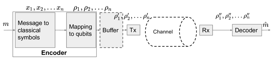
Figure 1: Qubit $\rho_{i}$ decoheres to $\rho_{i}^{\prime}$ while waiting in the buffer for transmission. This further decoheres to $\rho^{\prime\prime}_{i}$ while passing through the channel. Decoherence in the buffer depends on the waiting time and results in non-i.i.d. "effective" decoherence.

Next, we consider the setting in Fig. 1, where qubits are transmitted sequentially, and the qubits decohere as they wait to be transmitted. The extent of noise suffered by a particular qubit is a function of the waiting time spent by that qubit. In such a setting, the "effective" channel experienced by the qubits is non-stationary and has memory. We model this waiting time dependent noise using the quantum queue-channel framework, studied in [5]. Specifically, we study a symmetric GAD queue-channel with $n=1/2,$ and the parameter $p$ is made an explicit function of the waiting time $w$ of each qubit. Such a symmetric GAD queue channel is known to be additive, which enables the use of the capacity upper bound obtained in [5] for additive queue channels. Further, we propose a specific encoding for the GAD queue channel, which induces a binary symmetric classical queue channel. We show that an achievable rate of this binary symmetric queue channel matches the upper bound enforced by additivity arguments, thus settling the capacity of the GAD queue channel, and giving us a fully classical capacity achieving scheme for the encoder and decoder. Finally, we obtain useful insights for designing practical quantum communication systems by employing queuing theoretic analysis on the queue-channel capacity results.

The paper is organized as follows. In the Sec. 1.2 we discuss related work. To keep this discussion somewhat self-contained, in Sec. 2, we provide an extended discussion of induced channels, classical capacities of quantum channels, and non-i.i.d queue-channel capacities. In Sec. 3, we analyze the generalized amplitude damping channel (GADC). Here we discuss the capacity of various induced channels of GADC (see Figs. 2 and 3), and prove a key result (see Theorem 1) that Shannon capacity, Holevo capacity, and the classical capacity of the symmetric ($n=1/2$) GADC are all equal. In Sec. 4 we discuss the queue-channel capacity of the symmetric GADC. We offer useful design insights by analyzing and numerically plotting (see Fig. 4) the capacity expression. Sec. 5 contains a brief discussion and outlines potentially interesting future directions.

1.2 Related Work

Our work interleaves different aspects of quantum communication networks, from quantum Shannon theory to queuing theory. In quantum Shannon theory, one studies ultimate limits for transmitting information in the presence of quantum noise. The generalized amplitude damping channel (GADC) is a relevant model of noise in a variety of physical contexts including communication over optical fibers or free space [8, 9, 10, 11], $T_{1}$ relaxation due to coupling of spins with a high temperature environment [12, 13, 14], and super-conducting based quantum computing [15]. Quantum capacities of the i.i.d. GADC have been studied (see [7] and reference therein). Of particular interest to us are expressions for the Holevo information of the GADC, found in [16] using techniques from [17, 18], and channel parameters [7] where additivity of the GADC Holevo information is known.

While the primary focus of quantum Shannon theory [19] has been to study the classical and quantum capacities of stationary, memoryless quantum channels [20], recently there has been a spurt of activity in characterizing the capacities of quantum channels in non-stationary, correlated settings. We refer to [21] for a recent review of the different capacity results obtained in a context of quantum channels that are not independent or identical across channel uses. In particular, we focus on the quantum information-spectrum approach in [22], which provides bounds on the classical capacity of a general, non-i.i.d. sequence of quantum channels.

The idea of a quantum queue-channel was originally proposed in [23] as a way to model and study the effect of decoherence due to buffering or queuing in quantum information processing tasks. The classical capacity of quantum queue-channels has been studied for certain classes of quantum channels, and a general upper bound is known for additive quantum queue-channels [5]. The effect of queuing-dependent errors on classical channels has been studied earlier [24], with motivation drawn from crowd-sourcing. More recently, a dynamic programming based framework for characterising the queuing delay of quantum data with finite memory size has been proposed in [25]. Finally, we note that ideas of queuing theory have also been used to study aspects of entanglement distribution over quantum networks such as routing [26], switching, and buffering [27].

2 Preliminaries

2.1 Classical Channels

Consider a random variable $X$ that takes discrete values $x$ from a finite set ${\mathcal{X}}$ and another random variable $Y$ that takes discrete values $y$ from some finite set ${\mathcal{Y}}$. A discrete memoryless classical channel $N$ takes an input symbol $x$ to an output $y$ with conditional probability $p(y|x):=\Pr(Y=y|X=x)$. Sometimes it is convenient to represent a discrete memoryless classical channel $N$ as a transition matrix $M$ where $[M]_{yx}$ is $p(y|x)$. The channel $N$ is called memoryless because the probability distribution of the channel output $y$ depends on its current input $x$ and is conditionally independent of previous channel inputs. Noise is modelled by a channel mapping its inputs to a noisy output. When noise on several different inputs acts in such a way that noise on each input is described by the same discrete memoryless channel, one says the noise is independent and identically distributed (i.i.d.). In what follows we discuss rates for sending information in the presence of i.i.d. noise described by a discrete memoryless channel $N$.

We define the mutual the channel mutual information,

$${\mathcal{I}}^{(1)}(N)=\max_{p(x)}I(Y;X),$$ (1)

where $p(x):=\Pr(X=x)$ is a probability distribution over the input of $N$, and $I(Y;X)$ is the mutual information given by

$$I(Y;X):=H(X)+H(Y)-H(X,Y),$$ (2)

where $H(X)=-\sum_{x}p(x)\log_{2}p(x)$ is the Shannon entropy of the random variable $X$, and $H(X,Y)$ is the Shannon entropy of $Z=(X,Y)$. Channel mutual information (1) represents an achievable rate for sending information across $N$. Since $I(Y;X)$ is concave in $p(x)$ for fixed $p(y|x)$, ${\mathcal{I}}^{(1)}(N)$ can be computed numerically with relative ease [28, 29]. The channel mutual information is additive: ${\mathcal{I}}^{(1)}$ of a channel $N\times N^{\prime}$ formed by using two channels $N$ and $N^{\prime}$ together (sometimes called “used in parallel”) is the sum of ${\mathcal{I}}^{(1)}$ of the individual channels; that is,

$${\mathcal{I}}^{(1)}(N\times N^{\prime})={\mathcal{I}}^{(1)}(N)+{\mathcal{I}}^{(1)}(N^{\prime}).$$ (3)

Due to additivity, a classical channel $N$’s Shannon capacity,

$$C_{\text{Shan}}(N)=\lim_{k\mapsto\infty}\frac{1}{k}{\mathcal{I}}^{(1)}(N^{\times k}),$$ (4)

where $N^{\times k}$ represents $k$ parallel uses of the channel $N$, simplifies to

$$C_{\text{Shan}}(N)={\mathcal{I}}^{(1)}(N).$$ (5)

2.2 Induced Channels and Classical Quantum Channels

We now discuss the transmission of classical information using quantum states. We restrict ourselves to quantum systems described by some finite dimensional Hilbert space ${\mathcal{H}}$. Both pure and mixed states on these quantum systems can be described using unit-trace positive semi-definite operators (density operators) that belong to ${\mathcal{L}}({\mathcal{H}})$, the space of bounded linear operator on ${\mathcal{H}}$. Suppose classical information is encoded in quantum states using a fixed map ${\mathcal{E}}:{\mathcal{X}}\mapsto{\mathcal{L}}({\mathcal{H}})$, sometimes called a classical quantum channel which takes $x\in{\mathcal{X}}$ to a density operator $\rho(x)\in{\mathcal{L}}({\mathcal{H}})$. This classical information can be decoded by a map ${\mathcal{D}}:{\mathcal{L}}({\mathcal{H}})\mapsto{\mathcal{Y}}$ which represents measuring $\rho(x)$ to obtain an output $y\in{\mathcal{Y}}$. This measurement can be described using a POVM (a collection of positive operators in ${\mathcal{L}}({\mathcal{H}})$ that sum to the identity). Suppose the POVM $\{\Lambda(y)\}$ specifies ${\mathcal{D}}$; then any input $x\in{\mathcal{X}}$ is decoded as $y$ with conditional probability,

$$p(y|x)=\Pr(Y=y|X=x)={\rm Tr}\big{(}\Lambda(y)\rho(x)\big{)}.$$ (6)

This conditional probability defines an induced channel $N:{\mathcal{X}}\mapsto{\mathcal{Y}}$. Induced channels play a vital role in defining the capacity of quantum systems to send classical information. For a fixed encoding ${\mathcal{E}}$, when using a decoding ${\mathcal{D}}$, the induced channel capacity $C_{\text{Shan}}(N)$ represents a rate at which classical information can be sent using ${\mathcal{E}}$. The maximum rate of this type, sometimes called the Shannon capacity of ${\mathcal{E}}$,

$$C_{\text{Shan}}({\mathcal{E}})=\max_{{\mathcal{D}}}{\mathcal{I}}^{(1)}({\mathcal{N}})=\max_{{\mathcal{D}},p(x)}I(Y;X),$$ (7)

is obtained from maximizing the induced channel capacity over all possible induced channels, i.e., over all possible decoding ${\mathcal{D}}$. Not much is known about how to perform this optimization. For a fixed ${\mathcal{D}}$—that is, fixed $N$— ${\mathcal{I}}^{(1)}({\mathcal{N}})$ can be computed with relative ease (see comments below (1)). However, for a fixed $p(x)$ and output alphabet ${\mathcal{Y}}$, $I(Y;X)$ is convex in $p(y|x)$, and $p(y|x)$ is linear in the decoding POVM $\{\Lambda(y_{j})\}$ specifying ${\mathcal{D}}$. The resulting convexity of $I(Y;X)$ in ${\mathcal{D}}$, for fixed ${\mathcal{Y}}$ makes it non-trivial to numerically compute $C_{\text{Shan}}({\mathcal{E}})$.

A $k$-letter message $x^{k}=(x_{1},x_{2},\dots,x_{k})$ is encoded via ${\mathcal{E}}:{\mathcal{X}}\mapsto{\mathcal{L}}({\mathcal{H}})$, sometimes called a product encoding, into a product state $\rho_{k}:=\rho(x_{1})\otimes\rho(x_{2})\otimes\dots\otimes\rho(x_{k})$ and decoded via ${\mathcal{D}}:{\mathcal{L}}({\mathcal{H}})\mapsto{\mathcal{Y}}$, sometimes called a product decoding, using a product measurement on ${\mathcal{L}}({\mathcal{H}}^{\otimes k})$. Product decoding is a special case of joint decoding ${\mathcal{D}}_{k}:{\mathcal{L}}({\mathcal{H}}^{\otimes k})\mapsto{\mathcal{Y}}^{\times k}$ performed using a joint measurement POVM on ${\mathcal{L}}({\mathcal{H}}^{\otimes k})$ resulting in an element on $k$ copies of some classical alphabet ${\mathcal{Y}}^{\times k}$. Encoding ${\mathcal{E}}$ followed by joint decoding ${\mathcal{D}}_{k}$ results in an induced channel $N_{k}$. Maximizing the channel mutual information ${\mathcal{I}}(N_{k})$ over all decodings ${\mathcal{D}}_{k}$ defines ${\mathcal{I}}^{(k)}({\mathcal{E}})$. Due to the presence of entanglement in the joint decoding measurements, one may have ${\mathcal{I}}^{(k)}({\mathcal{E}})\geq k{\mathcal{I}}^{(1)}({\mathcal{E}})$. This inequality refers to the super-additivity of ${\mathcal{I}}^{(k)}({\mathcal{E}})$. Due to super-additivity, a proper definition of the capacity $C_{pj}$ of sending classical information using product encoding ${\mathcal{E}}$ and joint decoding ${\mathcal{D}}_{k}$ is given by a multi-letter formula,

$$C_{pj}=\lim_{k\mapsto\infty}\frac{1}{n}{\mathcal{I}}^{(k)}({\mathcal{E}}).$$ (8)

Remarkably, the Holevo-Schumacher-Westmoreland theorem [30, 31] gives the above multi-letter expression a single-letter form; that is,

$$C_{pj}({\mathcal{E}})=\chi^{(1)}({\mathcal{E}}):=\max_{\{p(x)\}}\chi\big{(}p(x),\rho(x)\big{)},$$ (9)

where the Holevo quantity,

$$\chi\big{(}p(x),\rho(x)\big{)}=S\big{(}\sum_{x\in{\mathcal{X}}}p(x)\rho(x)\big{)}-\sum_{x}p(x)S\big{(}\rho(x))\big{)},$$ (10)

and $S(\rho)=-{\rm Tr}(\rho\log\rho)$, is the von-Neumann entropy of a density operator $\rho$. Due to the close connection between $C_{pj}$ and $\chi$, sometimes $C_{pj}({\mathcal{E}})$ is also denoted by $C_{\chi}({\mathcal{E}})$. There are cases where $C_{\chi}({\mathcal{E}})$ is strictly greater than $C_{\text{Shan}}({\mathcal{E}})$ [32, 33]. However, much remains unknown about when and how such separations occurs.

2.3 Classical Capacities of a Quantum Channel

The quantum analog of a discrete memoryless classical channel is a (noisy) quantum channel ${\mathcal{B}}$. In general, if ${\mathcal{H}}_{a}$ and ${\mathcal{H}}_{b}$ are two finite dimensional Hilbert spaces, then the quantum channel ${\mathcal{B}}:{\mathcal{L}}({\mathcal{H}}_{a})\mapsto{\mathcal{L}}({\mathcal{H}}_{b})$ is a completely positive trace preserving (CPTP) map. In what follows, we discuss transmission of classical information using quantum states affected by a quantum channel ${\mathcal{B}}$ [34] (also see Ch.8 in [20]).

Sending classical information across ${\mathcal{B}}$ using product encoding ${\mathcal{E}}:{\mathcal{X}}\mapsto{\mathcal{L}}({\mathcal{H}}_{a})$ and product decoding ${\mathcal{D}}:{\mathcal{L}}({\mathcal{H}}_{b})\mapsto{\mathcal{Y}}$ results in an induced channel $N:{\mathcal{X}}\mapsto{\mathcal{Y}}$. Maximizing the channel mutual information of $N$ over ${\mathcal{E}}$ and ${\mathcal{D}}$ gives the product encoding-decoding capacity $C_{pp}({\mathcal{B}})$, also known as the Shannon capacity of ${\mathcal{B}}$,

$$C_{Shan}({\mathcal{B}})=\max_{{\mathcal{E}},{\mathcal{D}}}{\mathcal{I}}(N)=\max_{\{{\mathcal{E}},{\mathcal{D}}\}}\max_{p(x)}I(Y;X).$$ (11)

The Shannon capacity is bounded from above by the product encoding joint decoding capacity $C_{pj}({\mathcal{B}})$, sometimes called the Holevo capacity or the product state capacity. Using a procedure similar to the one above (8), the capacity $C_{pj}({\mathcal{B}})$ can be defined with the aid of induced channels generated from product encoding but joint decoding. Such a definition results in multi-letter expression of the type (9) with a single-letter characterization,

$$C_{pj}({\mathcal{B}})=\chi^{(1)}({\mathcal{B}}):=\max_{\{\rho_{a}(x),p(x)\}}\chi\big{(}p(x),\rho_{b}(x)\big{)},$$ (12)

where $\rho_{b}(x)={\mathcal{B}}(\rho_{a}(x))$.

The product state capacity $\chi^{(1)}({\mathcal{B}})$ can be further generalized to include the possibility of using joint encoding ${\mathcal{E}}_{k}:{\mathcal{X}}^{\times k}\mapsto{\mathcal{L}}({\mathcal{H}}_{a}^{\otimes k})$ at the channel input and joint decoding ${\mathcal{D}}_{k}:{\mathcal{L}}({\mathcal{H}}^{\otimes k}_{b})\mapsto{\mathcal{Y}}^{\times k}$ at the output. This encoding-decoding results in an induced channel $\tilde{N}_{k}:X^{\times k}\mapsto Y^{\times k}$. Maximizing the mutual information of this induced channel over all encoding ${\mathcal{E}}_{k}$ and decoding ${\mathcal{D}}_{k}$ gives $\tilde{\mathcal{I}}^{k}({\mathcal{B}})$. Due to the presence of entanglement at the encoding, one may have super-additivity of the form $\tilde{\mathcal{I}}^{k}({\mathcal{B}})\geq k\tilde{\mathcal{I}}({\mathcal{B}})$. Due to this super-additivity, the joint encoding-decoding capacity $C_{jj}({\mathcal{B}})$, sometimes called the classical capacity of ${\mathcal{B}}$, is defined by a multi-letter expression of the form (8). The capacity $C_{jj}({\mathcal{B}})$ can be characterized using the product state capacity (12) as follows,

$$C_{jj}({\mathcal{B}})=\chi({\mathcal{B}}):=\underset{k\mapsto\infty}{\lim}\frac{1}{k}\chi^{(1)}({\mathcal{B}}^{\otimes k}).$$ (13)

In general, the limit in (13) is required because the product state capacity can be non-additive [35]; that is, for any two quantum channels ${\mathcal{B}}$ and ${\mathcal{B}}^{\prime}$, the inequality,

$$\chi^{(1)}({\mathcal{B}}\otimes{\mathcal{B}}^{\prime})\geq\chi^{(1)}({\mathcal{B}})+\chi^{(1)}({\mathcal{B}}^{\prime}),$$ (14)

can be strict. For certain special classes of channels, the Holevo information is known to be additive; that is, the inequality above becomes an equality when ${\mathcal{B}}$ is any channel and ${\mathcal{B}}^{\prime}$ belongs to a special class of channels. These special classes are unital qubit channels [36], depolarizing channels [37], Hadamard channels [38], and entanglement breaking channels [39].

2.4 Classical capacity of non-i.i.d. quantum channels

As mentioned in Sec. 1, the effective channel seen by qubits in the presence of decoherence in the transmission buffer is non-i.i.d. Characterizing the capacity is a harder problem in such a setting. In the classical setting, a capacity formula for this general non-i.i.d. setting was obtained using the information-spectrum method [40, 41]. This technique was adapted to the quantum setting in [22], and a general capacity formula was obtained for the classical capacity of a quantum channel.

2.4.1 The Quantum inf-information rate

Recall that a quantum channel is defined as a completely positive, trace-preserving map ${\mathcal{B}}:{\mathcal{H}}_{a}\mapsto{\mathcal{H}}_{b}$ from the "input" Hilbert space ${\mathcal{H}}_{a}$ to the "output" Hilbert space ${\mathcal{H}}_{b}$. Consider a sequence of quantum channels $\vec{\mathcal{N}}\equiv\{\mathcal{N}^{(n)}\}_{n=1}^{\infty}$. Let $\vec{P}$ denote the totality of sequences $\{P^{n}(X^{n})\}_{n=1}^{\infty}$ of probability distributions (with finite support) over input sequences $X^{n}$, and $\vec{\rho}$ denote the sequences of states $\rho_{X^{n}}$ corresponding to the encoding $X^{n}\rightarrow\rho_{X^{n}}$. For any $a\in\mathbb{R}^{+}$ and $n$, we define the operator,

$$\Gamma_{\{P^{n}(X^{n}),\rho_{X^{n}}\}}(a)=\mathcal{N}^{(n)}(\rho_{X^{n}})-e^{an}\sum_{X^{n}\in\mathcal{X}^{(n)}}P^{n}(X^{n})\mathcal{N}^{(n)}(\rho_{X^{n}}).$$

Further, let $\{\Gamma_{\{P^{n}(X^{n}),\rho_{X^{n}}\}}(a)>0\}$ denote the projector onto the positive eigenspace of the operator $\Gamma_{\{P^{n}(X^{n}),\rho_{X^{n}}\}}(a)$.

Definition 1.

The quantum inf-information rate [22] $\underline{\mathbf{I}}(\,\{\vec{P},\vec{\rho}\,\},\vec{\mathcal{N}}\,)$ is defined as,

$$\underline{\mathbf{I}}(\,\{\vec{P},\vec{\rho}\,\},\vec{\mathcal{N}}\,)=\sup\left\{a\in\mathbb{R}^{+}\left|\lim_{n\rightarrow\infty}\sum_{X^{n}\in\mathcal{X}^{(n)}}P^{n}(X^{n})\operatorname{tr}\left[\mathcal{N}^{(n)}(\rho_{X^{n}})\left\{\Gamma_{\{P^{n}(X^{n}),\rho_{X^{n}}\}}(a)>0\right.\right\}\right]=1\right\}.$$ (15)

This is the quantum analogue of the classical inf-information rate originally defined in [40, 41]. The central result of [22] is to show that the classical capacity of the channel sequence $\vec{\mathcal{N}}$ is given by

$$C=\sup_{\{\vec{P},\vec{\rho}\}}\underline{\mathbf{I}}(\{\vec{P},\vec{\rho}\},\vec{\mathcal{N}}).$$

3 Generalized Qubit Amplitude Damping

The generalized qubit amplitude damping channel (GADC) ${\mathcal{A}}_{p,n}:{\mathcal{L}}({\mathcal{H}}_{a})\mapsto{\mathcal{L}}({\mathcal{H}}_{b})$ is a two parameter family of channels where the parameters $p$ and $n$ are between zero and one. The channel has a qubit input and qubit output—$d_{a}=d_{b}=2$— and its superoperator has the form,

$${\mathcal{A}}_{p,n}(\rho)=\sum_{i=0}^{3}K_{i}\rho K_{i}^{{\dagger}},$$ (16)

where

$$K_{0} =\sqrt{1-n}(|0\rangle\langle 0|+\sqrt{1-p}|1\rangle\langle 1|), K_{1} =\sqrt{p(1-n)}|0\rangle\langle 1|,$$ (17)

$$K_{2} =\sqrt{n}(\sqrt{1-p}|0\rangle\langle 0|+|1\rangle\langle 1|),\quad\text{and} K_{3} =\sqrt{pn}|1\rangle\langle 0|$$ (18)

are Kraus operators. The GADC (16) can also be expressed as

$${\mathcal{A}}_{p,n}=(1-n){\mathcal{A}}_{p,0}+n{\mathcal{A}}_{p,1}.$$ (19)

The above representation provides the following insightful interpretation. The parameter $n$ represents the mixing of ${\mathcal{A}}_{p,0}$ with ${\mathcal{A}}_{p,1}$, where each channel ${\mathcal{A}}_{p,i}$ ($i=0$ or $1$) is an amplitude damping channel that favours the state $[i]$ by keeping it fixed and maps the orthogonal state $[1-i]$ to $[i]$ with damping probability $p$. When $n=1/2$, we get equal mixing of both ${\mathcal{A}}_{p,0}$ and ${\mathcal{A}}_{p,1}$. This equal mixing represents noise where each state $[i]$ ($i=0,1$) is mapped to itself with probability $p$ and to $[1-i]$ with probability $1-p$; in other words, this $n=1/2$ noise treats both $[0]$ and $[1]$ identically. However, when $n$ is not half, the action of ${\mathcal{A}}_{p,n}$ on $[0]$ is different from its action on $[1]$. In particular, $[0]$ is mapped to itself with probability $1-pn$ and to $[1]$ with probability $pn$, and $[1]$ is mapped to itself with probability $1-p(1-n)$ and to $[0]$ with probability $p(1-n)$.

Any qubit density operator can be written in the Bloch parametrization,

$$\rho(\textbf{r})=\frac{1}{2}(I+\textbf{r}.\vec{\sigma}):=\frac{1}{2}(I+x\sigma^{x}+y\sigma^{y}+z\sigma^{z}),$$ (20)

where the Bloch vector $\textbf{r}=(x,y,z)$ has norm $|\textbf{r}|\leq 1$,

$$\sigma^{x}=\left(\begin{matrix}0&1\\ 1&0\end{matrix}\right),\quad\sigma^{y}=\left(\begin{matrix}0&-i\\ i&0\end{matrix}\right),\quad\text{and}\quad\sigma^{z}=\left(\begin{matrix}1&0\\ 0&-1\end{matrix}\right)$$ (21)

are the Pauli matrices, written in the standard basis $\{|0\rangle,|1\rangle\}$. Using the Bloch parametrization, the entropy

$$S\big{(}\rho(\textbf{r})\big{)}=h\big{(}(1-|\textbf{r}|)/2\big{)},$$ (22)

where $h(x):=-[x\log x+(1-x)\log(1-x)]$ is the binary entropy function and $|\textbf{r}|=\sqrt{\textbf{r}.\textbf{r}}$ is the norm of r. An input density operator $\rho(\textbf{r})$ is mapped by ${\mathcal{A}}_{p,n}$ to an output density operator with Bloch vector,

$$\textbf{r}^{\prime}=(\sqrt{1-p}x,\sqrt{1-p}y,(1-p)z+p(1-2n)).$$ (23)

The GADC is unital at $n=1/2$; that is, ${\mathcal{A}}_{p,\frac{1}{2}}(I)=I$. The GADC is entanglement breaking [7] when

$$2(\sqrt{2}-1)\leq p\leq 1\quad\text{and}\quad\frac{1}{2}(1-l(p))\leq n\leq\frac{1}{2}(1+l(p)),$$ (24)

where $l(p)=\sqrt{\frac{p^{2}+4p-4}{p^{2}}}$. The Holevo capacity of unital qubit channels and entanglement breaking channels is additive; as a result, when $n=1/2$ and when the values of parameters $p$ and $n$ satisfy (24), the Holevo information of the generalized amplitude damping channel equals the classical capacity of the channel. For other values of $p$ and $n$, the classical capacity of the GADC is not known because for these parameter values, the Holevo information of the channel is not known to be additive or non-additive. The actual value of the Holevo information can be computed numerically. Next, we briefly discuss this numerical calculation.

3.1 Holevo Information

Let $[\alpha_{+}]$ and $[\alpha_{-}]$ be projectors on states with Bloch vector

$$\textbf{r}_{+}=(\sqrt{1-z^{2}},0,z),\quad\text{and}\quad\textbf{r}_{-}=(-\sqrt{1-z^{2}},0,z),$$ (25)

respectively; here $-1\leq z\leq 1$. Notice, $[\alpha_{+}]$ and $[\alpha_{-}]$ are not orthogonal, except when $z=0$. It has been shown [16] that the Holevo information,

$$\chi^{(1)}({\mathcal{A}}_{p,n})=\max_{\{-1\leq z\leq 1\}}\;S\big{(}{\mathcal{A}}_{p,n}(\sigma)\big{)}-[S\big{(}{\mathcal{A}}_{p,n}([\alpha_{+}])\big{)}+S\big{(}{\mathcal{A}}_{p,n}([\alpha_{-}])\big{)}]/2,$$ (26)

where $\sigma=([\alpha_{+}]+[\alpha_{-}])/2$. In the above equation, the optimizing $z$ has the value

$$z^{*}=\frac{u-p(1-2n)}{1-p},$$ (27)

where $u$ comes from solving,

$$\big{(}pu-p^{2}(1-2n)-p(1-p)(1-2n)\big{)}f^{\prime}(r^{*})=-r^{*}(1-\gamma)f^{\prime}(u),$$ (28)

with

$$f(x) :=(1+x)\log_{2}(1+x)+(1-x)\log_{2}(1-x),$$ (29)

$$f^{\prime}(x) =\log_{2}\Big{(}\frac{1+x}{1-x}\Big{)},\quad\text{and}$$ (30)

$$r^{*} :=\sqrt{1-p-\frac{\big{(}u-p(1-2n)\big{)}^{2}}{1-p}+u^{2}}.$$ (31)

Using the value of $z^{*}$ in (27) gives,

$$\chi^{(1)}({\mathcal{A}}_{p,n})=\frac{1}{2}\big{(}f(r^{*})-\log_{2}(1-u^{2})-uf^{\prime}(u)\big{)}.$$ (32)

Solving (24) for $n\leq 1/2$ gives a range,

$$p^{*}\leq p\leq 1,$$ (33)

where the GADC in entanglement breaking. Here the value,

$$p^{*}=\max\Big{(}2(\sqrt{2}-1),\frac{\sqrt{1+4n(1-n)}-1}{2n(1-n)}\Big{)}.$$ (34)

As indicated earlier, entanglement breaking channels have additive Holevo capacity. Thus, when $p$ satisfies (33), the GADC has additive Holevo capacity. While the Holevo information $\chi^{(1)}({\mathcal{A}}_{n,p})$ gives the product state classical channel capacity, it doesn’t give an explicit encoding and decoding that achieves this capacity. In what follows, we construct explicit encoding and decodings—in other words, we construct induced classical channels, and compare the capacity of these channels to the product state classical capacity $\chi^{(1)}({\mathcal{A}}_{n,p})$. For $n=1/2$, we find the optimal encoding and decoding which achieves $\chi^{(1)}({\mathcal{A}}_{1/2,p})$ for all $0\leq p\leq 1$.

3.2 Induced Channels

To obtain an induced channel for ${\mathcal{A}}_{p,n}$ one must choose an encoding and decoding. To choose an encoding, ${\mathcal{E}}:x\mapsto\rho(x)$, one fixes a set of input states $\{\rho(x)\}$. To choose a decoding, ${\mathcal{D}}:\rho(x)\mapsto y$, one fixes an output measurement POVM $\{\Lambda(y)\}$. Together the encoding-decoding results in an induced channel with conditional probability $p(y|x)={\rm Tr}(\rho(x)\Lambda(y))$. A priori, there is no clear choice for these input states and output measurement. However, the generalized qubit amplitude damping channel satisfies an equation

$${\mathcal{A}}_{p,n}\big{(}\sigma^{z}_{a}\;\rho\;(\sigma^{z}_{a})^{{\dagger}}\big{)}=\sigma^{z}_{b}\;{\mathcal{A}}_{p,n}(\rho)\;(\sigma^{z}_{b})^{{\dagger}},$$ (35)

where the subscripts $a$ and $b$ on the Pauli operator $\sigma^{z}$ signify the space on which the operator acts. The above equation implies that the generalized amplitude damping channel has a rotational symmetry around the $z$-axis. Using this rotational symmetry and the fact that ${\mathcal{A}}_{p,n}$ is a qubit input-output channel one may choose an encoding ${\mathcal{E}}:x\mapsto\rho(x)$ where $x=0$ or $1$ and $\{\rho(x)\}$ are two orthogonal input states that remain unchanged under the $\sigma^{z}_{a}$ symmetry operations; that is, $\rho(x)=[x]$. To decode, one may apply a protocol for correctly identifying a state chosen uniformly from a set of two known states ${\mathcal{A}}_{p,n}([0])$ and ${\mathcal{A}}_{p,n}([1])$ with highest probability. This protocol comes from the theory of quantum state discrimination [42]. It uses a POVM with two elements $\{E,I_{b}-E\}$, where $E$ is a projector onto the space of positive eigenvalues of ${\mathcal{A}}_{p,n}([0])-{\mathcal{A}}_{p,n}([1])$. An unknown state, either ${\mathcal{A}}_{p,n}([0])$ or ${\mathcal{A}}_{p,n}([1])$ with equal probability, is measured using the POVM. If the outcome corresponding to $E$ occurs, the unknown state is guessed to be ${\mathcal{A}}_{p,n}([0])$; otherwise, the guess is ${\mathcal{A}}_{p,n}([1])$. In the present case, a simple calculation shows that $E=[0]$.

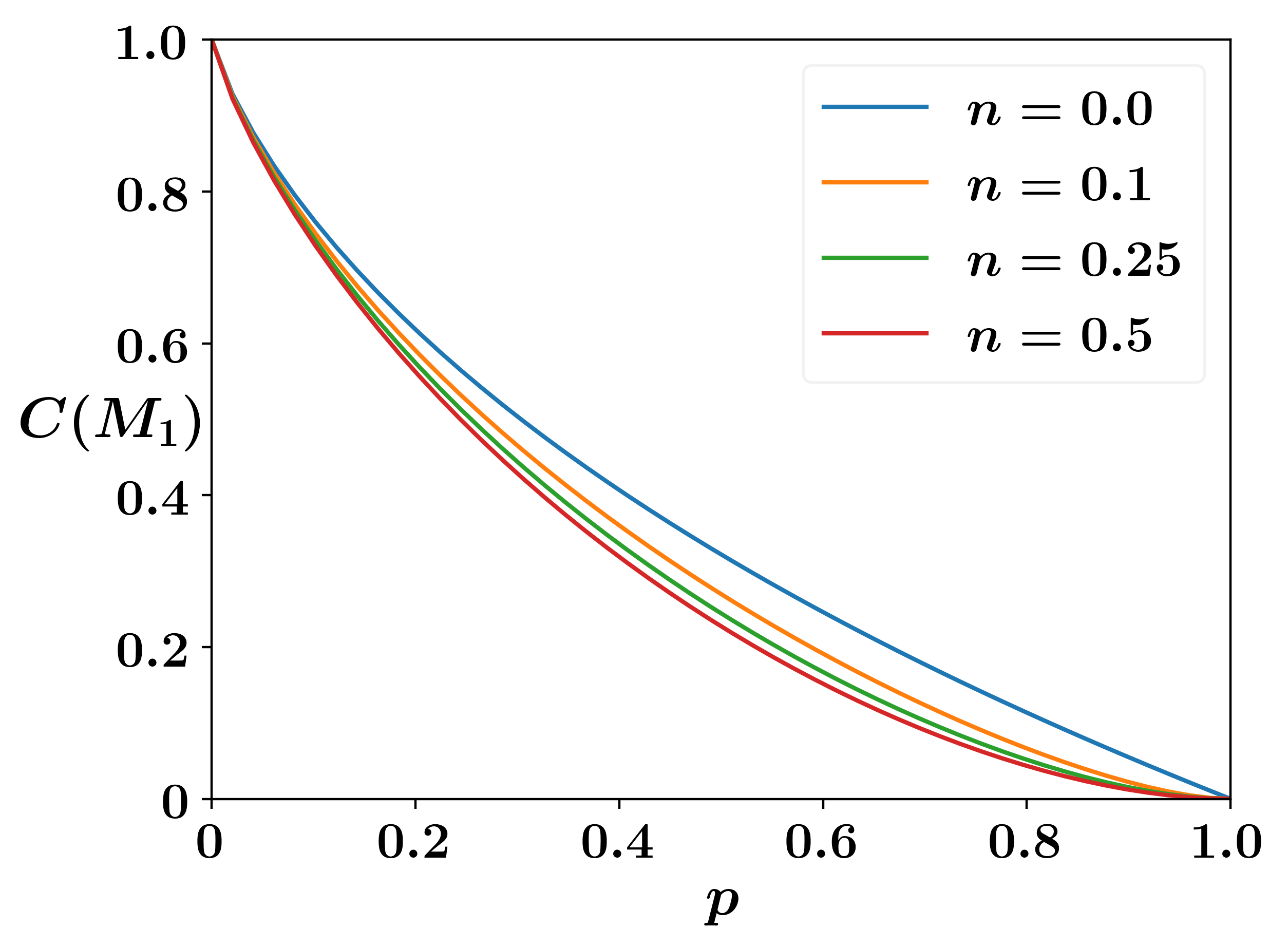
(a) The capacity $C(M_{1})$ of the induced channels $M_{1}$
as a function of $p$ for various values of the parameter $n$.
This channel $M_{1}$ is defined by transition probability
matrix $P^{\prime}$ in (36).

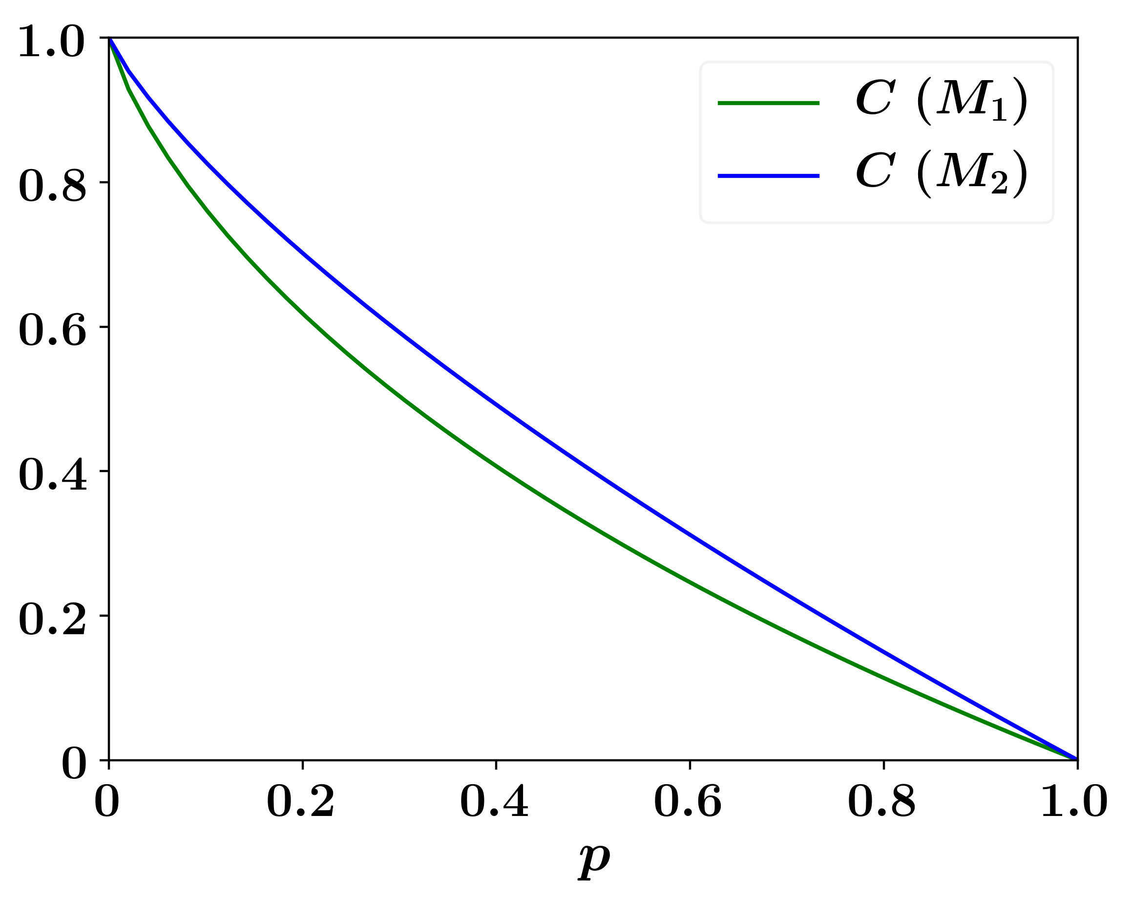
(b) As a function of $p$, the capacity $C(M_{1})$ is largest when $n=1/2$. This largest capacity is plotted in green and $C(M_{2})$ is plotted in blue. The induced channels $M_{1}$ and $M_{2}$, are defined by transition probability matrices $P^{\prime}$ and $Q(0)$ in (36) and (38), respectively.

Figure 2: Capacities of induced channels 

The state discrimination protocol outlined above can be used as the decoding map ${\mathcal{D}}:\rho(x)\mapsto y$, which measures $\rho(x)$ using the POVM $\{\Lambda(y)=[y]\}$ and returns $y\in\{0,1\}$ with conditional probability ${\rm Tr}(\rho(x)\Lambda(y))$. This choice of decoding, together with the encoding, ${\mathcal{E}}:x\mapsto[x]$, results in an induced channel $M_{1}$ with transition probability matrix

$$P^{\prime}=\left(\begin{matrix}1-pn&p(1-n)\\ pn&1-p(1-n)\end{matrix}\right).$$ (36)

This induced channel $M_{1}$ corresponding to the above matrix $P^{\prime}$ is a binary asymmetric channel that flips $x=00$ to $x=1$ with probability $pn$ but flips $x=1$ to $x=0$ with probability $p(1-n)$. The capacity of $M_{1}$ is given by

$$C(M_{1})=\max_{0\leq a\leq 1}h(r)-(1-a)h(pn)-ah\big{(}p(1-n)\big{)},$$ (37)

where $r=(1-pn)-a(1-p)$. From the above equation, it is clear that $C(M_{1})$ is unchanged when $n$ is replaced with $1-n$. We restrict ourselves to $0\leq n\leq 1/2$. As can be seen from Fig. 2(a), $C(M_{1})$ decreases with $n$ for $0\leq n\leq 1/2$.

Next, we consider a different induced channel where the encoding is performed using possibly non-orthogonal states and decoding is performed using a measurement designed to distinguish these encoded states at the channel output with maximum probability. The encoding maps $x=0$ and $x=1$ to $[\alpha_{+}]$ and $[\alpha_{-}]$ (defined via eq. (25)), respectively. The decoding is performed using a POVM $\{\Lambda(y)\}$ where $\Lambda(y)$ at $y=0$ is the projector onto the space of positive eigenvalues of ${\mathcal{A}}_{p,n}([\alpha_{+}])-{\mathcal{A}}_{p,n}([\alpha_{-}])$. This projector is simply $[x+]$, where $|x+\rangle:=(|0\rangle+|1\rangle)\sqrt{2}$. This encoding-decoding scheme results in a one-parameter family of induced channels $M_{2}(z)$. This family of channels has a transition matrix

$$Q(z)=\left(\begin{matrix}q(z)&1-q(z)\\ 1-q(z)&q(z)\end{matrix}\right),$$ (38)

where $q(z)=(1-a(z)\sqrt{1-p})/2$, and $a(z)=\sqrt{1-z^{2}}$. For any $z$, the induced channel $M_{2}(z)$ is a binary symmetric channel with flip probability $q(z)$. Interestingly, this family of induced channels coming from the GADC ${\mathcal{A}}_{p,n}$ does not depend on the parameter $n$ in the channel. The Shannon capacity of $M_{2}(z)$ is simply

$$C(M_{2}(z))=\;1-h\big{(}q(z)\big{)}.$$ (39)

For a fixed $p$, one can easily show that $C(M_{2}(z))$ is maximum when $z=0$; thus, $M_{2}=M_{2}(0)$ has the largest Shannon capacity among the one-parameter family of induced channels $M_{2}(z)$. This induced channel $M_{2}$ is simply a binary symmetric channel with flip probability $q=(1-\sqrt{1-p})/2$. We compare the capacity of $M_{2}$ with that of $M_{1}$ at $n=0$, defined earlier (see Fig. 2(b)) to find that

$$C(M_{2})\geq C(M_{1}),$$ (40)

for all $p$ and $n$. In Fig. 3, we compare the capacity $C(M_{2})$ of the induced channel $M_{2}$ with the Holevo information of the GADC for various values $n$. We numerically find that for values of $n<1/2$ and $0<p<1$, $C(M_{2})<\chi^{(1)}({\mathcal{A}}_{p,n})$. Next we focus on ${\mathcal{A}}_{p,1/2}$, the GADC at $n=1/2$.

Theorem 1.

For the $n=1/2$ GADC, ${\mathcal{A}}_{p,1/2}$, the Shannon capacity, product-state capacity, and classical capacity are all equal to that of a binary symmetric channel with flip probability $q=(1-\sqrt{1-p})/2$.

Proof.

Our proof has two key ingredients: first is a well-known additivity of $\chi^{(1)}({\mathcal{A}}_{p,1/2})$ and second is an argument to show that capacity of a binary symmetric induced channel of ${\mathcal{A}}_{p,1/2}$ bounds $\chi^{(1)}({\mathcal{A}}_{p,1/2})$ from above and below.

Notice the $n=1/2$ GADC, ${\mathcal{A}}_{p,1/2}$ is unital. As a result, the channel’s Holevo information is additive and equals the channel’s classical capacity; that is,

$$\chi({\mathcal{A}}_{p,1/2})=\chi^{(1)}({\mathcal{A}}_{p,1/2}).$$ (41)

The Holevo information $\chi^{(1)}({\mathcal{A}}_{p,1/2})$ is the product-state classical capacity of ${\mathcal{A}}_{p,1/2}$. This product state capacity bounds the Shannon capacity of ${\mathcal{A}}_{p,1/2}$ from above. In turn, this Shannon capacity upper bounds the capacity of any induced channel of ${\mathcal{A}}_{p,1/2}$ that uses product encoding and decoding. Since the induced channel $M_{2}$, defined in (39), uses product encoding and product decoding,

$$C(M_{2})\leq C_{\text{Shan}}({\mathcal{A}}_{p,1/2})\leq\chi^{(1)}({\mathcal{A}}_{p,1/2}).$$ (42)

This induced channel $M_{2}$ is a binary symmetric channel with flip probability $q=(1-\sqrt{1-p})/2$. The channel’s capacity is

$$C(M_{2})=1-h(q),$$ (43)

where $h$ is the binary entropy function. We now show this capacity $C(M_{2})$ bounds $\chi^{(1)}({\mathcal{A}}_{p,1/2})$ from above. From eq. (26),

$$\chi^{(1)}({\mathcal{A}}_{p,1/2})=\max_{-1\leq z\leq 1}\{S\big{(}{\mathcal{A}}_{p,1/2}(\sigma)\big{)}-[S\big{(}{\mathcal{A}}_{p,1/2}([\alpha_{+}])\big{)}+S\big{(}{\mathcal{A}}_{p,1/2}([\alpha_{-}])\big{)}]/2\}.$$ (44)

Using (25),(23), and (22) we find that

$$S\big{(}{\mathcal{A}}_{p,1/2}([\alpha_{+}])\big{)}=S\big{(}{\mathcal{A}}_{p,1/2}([\alpha_{-}])\big{)}=h\big{(}(1-|\textbf{r}_{b}|)/2\big{)},$$ (45)

where $\textbf{r}_{b}=\big{(}\sqrt{(1-p)(1-z^{2})},0,(1-p)z\big{)}$. Using (45) and (44) we bound the value of $\chi^{(1)}({\mathcal{A}}_{p,1/2})$ from above as follows:

$$\chi^{(1)}({\mathcal{A}}_{p,1/2})\leq\max_{-1\leq z\leq 1}S\big{(}{\mathcal{A}}_{p,1/2}(\sigma)\big{)}-\min_{-1\leq z\leq 1}h\big{(}(1-|\textbf{r}_{b}|)/2\big{)}$$ (46)

Notice (1) the maximum value of $S\big{(}{\mathcal{A}}_{p,1/2}(\sigma)\big{)}$ is at most $1$ because ${\mathcal{A}}_{p,1/2}$ has a qubit output; (2) $h((1-|\textbf{r}_{b}|)/2)$ is monotonically decreasing in $|\textbf{r}_{b}|$ and takes its minimum value $h\big{(}(1-\sqrt{1-p})/2\big{)}$ at $z=0$. Using these two facts in (46) along with (43),

$$\chi^{(1)}({\mathcal{A}}_{p,1/2})\leq 1-h(q)=C(M_{2}).$$ (47)

Together, (47), (42), and (41) prove

$$C(M_{2})=C_{Shan}({\mathcal{A}}_{p,1/2})=\chi^{(1)}({\mathcal{A}}_{p,1/2})=\chi({\mathcal{A}}_{p,1/2})=1-h(q),$$ (48)

where $q=(1-\sqrt{1-p})/2$. ∎

This equality (48) above shows that the induced channel $M_{2}$, obtained from product encoding and product decoding, achieves not only the Shannon capacity $C_{Shan}({\mathcal{A}}_{p,1/2})$ but also the product state capacity of ${\mathcal{A}}_{p,1/2}$. A by-product is an alternate proof for the product state capacity $\chi^{(1)}({\mathcal{A}}_{1/2,p})$ expression (see Ex.8.1 in [20]). Even more notably, the product state capacity in general allows for joint decoding of its product state inputs; however, we find that product decoding of the type in the induced channel $M_{2}$ suffices to achieve this capacity. For ${\mathcal{A}}_{p,1/2}$ the product state capacity $\chi^{(1)}({\mathcal{A}}_{p,1/2})$ is additive and equals the ultimate channel capacity $\chi({\mathcal{A}}_{p,1/2})$. This ultimate capacity allows for the more general joint encoding and joint decoding, yet the additivity of $\chi^{(1)}({\mathcal{A}}_{p,1/2})$, along with the equality in (48), show how this ultimate capacity is simply achieved using product encoding and product decoding.

Figure 3: The difference $\Delta=\chi^{(1)}({\mathcal{A}}_{p,n})-C(N_{2})$ as a function of $p$ for various values of the parameter $n$. For each $n$, the colored triangle indicates the value of $p^{*}$ above which $\chi^{(1)}({\mathcal{A}}_{p,n})$ is additive.

In what follows, we focus on the $n=1/2$ GADC ${\mathcal{A}}_{p,1/2}$. As discussed below (19), this channel describes noise in which both computational basis states $|0\rangle$ and $|1\rangle$ are treated on equal footing. When information about which of these computational basis states decays faster than the other, the GADC with $n\neq 1/2$ is an apt noise model. However when such information is unavailable, or when it is known that both computational basis states decay but the maximally mixed state doesn’t, one uses the $n=1/2$ GADC. One simple example of such noise is the qubit thermal channel (analogous to the bosonic thermal channel [7, 13, 14]) in which the channel environment is represented by the maximally mixed state. Another simple example is the effect of dissipation to an environment at a finite temperature [43].

4 Decoherence in Buffer: A Queue-channel Approach

For communicating a message over a GAD channel, a sequence of product quantum states has to be transmitted serially. In an idealized i.i.d. setting, it is implicitly assumed that the transmission of each state takes a fixed amount of time and that the qubits are prepared accordingly to avoid any buffering. However, in practice, preparation times as well as transmission (and reception) times are stochastic due to the inherent quantum physical nature of the devices. This naturally leads to queuing of qubits at the buffer of the transmitter, and the queued qubits decohere due to their interactions with the environment of the buffer. A schematic of this setting is presented in Fig. 1.

Note that the decoherence while waiting in the buffer is in addition to the decoherence experienced by the qubits while passing through the channel. The decoherence experienced by a qubit in the buffer depends on its waiting time in the buffer: the longer the wait, the worse the decoherence. Due to the queuing dynamics, the waiting times of the qubits are different and non i.i.d. Hence, the effective decoherence experienced by the qubits are also non i.i.d..

Most information theoretic channel models assume an idealized scenario without any decoherence in the transmission buffer. In Sec. 3, we studied the capacity of GAD channels assuming such an idealized scenario and showed that non-entangled encoding and decoding schemes can achieve the capacity of symmetric ($n=\frac{1}{2}$) GADC. In this section, we introduce a GAD queue-channel that can model both channel and buffer decoherence. The concept of a quantum queue-channel was introduced in [5] by adapting a related classical notion from [24]. Building on the results in Sec. 3, we characterize the capacity of GAD queue-channels and show that non-entangled encoding and decoding schemes achieve that capacity.

4.1 Symmetric GAD queue-channel

For a symmetric GADC, the parameter $p$ captures the level of damping experienced by a qubit while interacting with an environment. In the absence of buffer decoherence, $p$ depends on the flight time $T_{f}$ through the channel and the physical parameters of the channel. Similarly, the level of damping experienced in the buffer depends on the waiting time in the buffer $W$ and the physical parameters of the buffer. Hence, the effective GADC parameter experienced by a qubit is a function $g(T_{f},W)$ of its waiting time and its flight time, where the form of $g(\cdot)$ depends on the physical parameters of the channel and the buffer. As the flight time is almost deterministic, for simplicity of notations we denote this function by $p_{\mbox{eff}}(W)$.

In optical quantum communication, the prevalent form of quantum communication, often the transmission channel and the buffer are both made of optical fibers. Also, in practice, it is mostly the case that the noise treats both $[0]$ and $[1]$ identically. So, it is natural to assume that the mixing parameter $n$ is $\frac{1}{2}$ and $n$ does not depend on the waiting time. On the other hand, the damping parameter $p$ depends on the time of interaction with the environment. These motivated the above modeling assumptions regarding symmetric GAD queue-channel with waiting time dependent damping parameter $p_{\mbox{eff}}(W)$. However, for other modes of quantum communication, the models for buffer decoherence and channel decoherence can be different. This would be an interesting direction for future exploration.

A classical message is encoded into a sequence of classical states $x_{1},x_{2},\ldots,x_{k}$, which in turn is transmitted as a sequence of quantum states or qubits $\rho_{1},\rho_{2},\ldots,\rho_{k}$. Effectively, qubit $i$ is received at the receiver after its passage through a symmetric GADC with parameter $p_{\mbox{eff}}(W_{i})$, where $W_{i}$ is the time between the preparation of the $i$th qubit and its transmission. Given the knowledge of $W_{1},W_{2},\ldots,W_{k}$ at the receiver, qubits experience independent but not identically distributed symmetric generalized amplitude damping decoherence.

We complete the description of the combined channel with the mathematical model of the queuing system that gives rise to the waiting time sequence. The buffering process is modeled as a continuous-time single-server queue. To be specific, the single-server queue is characterised by (i) A server that processes the qubits in the order in which they arrive, that is in a First Come First Served (FCFS) fashion, and (ii) An "unlimited buffer" — that is, there is no limit on the number of qubits that can wait to be transmitted. We denote the time between preparation of the $i$th and $i+1$th qubits by $A_{i}$, where $A_{i}$ are i.i.d. random variables. These $A_{i}$s are viewed as inter-arrival times of a point process of rate $\lambda,$ where $\mathbb{E}[A_{i}]=1/\lambda.$ The "service time," or the time taken to transmit qubit $i,$ is denoted by $S_{i}$, where $\{S_{i}\}$ are also assumed to be i.i.d. random variables, independent of the inter-arrival times $A_{i},i\geq 1$. The "service rate" of the qubits is denoted by $\mu=1/\mathbb{E}[S_{i}].$ We assume that $\lambda<\mu$ (i.e., mean transmission time is strictly less than the mean preparation time) to ensure stability of the queue. Qubit $1$ has a waiting time $W_{1}=S_{1}$. The waiting times of the other qubits can be obtained using the well known Lindley’s recursion:

$$W_{i+1}=\max(W_{i}-A_{i},0)+S_{i+1}.$$

In queuing parlance, the above system describes a continuous-time $G/G/1$ queue. Under mild conditions, the sequence $\{W_{i}\}$ for a stable $G/G/1$ queue is ergodic, and reaches a stationary distribution $\pi.$ We assume that the waiting times $\{W_{i}\}$ of the qubits are not available at the transmitter during encoding, but are available at the receiver during decoding.

An important difference between the queue-channel introduced above and the usual i.i.d. channels is that this channel is a part of continuous time dynamics. Hence, the usual notion of capacity per channel use for i.i.d. channels is not pertinent here. As mentioned before, the above channel model is closely related to quantum queue-channels studied in [5]. So, we first do a short review of the notion of capacity per unit time and some relevant capacity results in [5].

4.1.1 Classical capacity of additive quantum queue-channels

Definition 2.

A rate $R$ is called an achievable rate for a quantum queue-channel if there exists a sequence of $(n,2^{RT_{n}})$ quantum codes with probability of error $P_{e}^{(n)}\to 0$ as $n\to\infty$ and $\mathbf{E}\left[\sum_{i=1}^{n-1}A_{i}+W_{n}\right]\leq T_{n}$.

Definition 3.

The information capacity of the queue-channel is the supremum of all achievable rates for a given arrival and service process, and is denoted by $C$ bits per unit time.

Note that the information capacity of the queue-channel depends on the arrival process, the service process, and the noise model. We assume that the receiver knows the realizations of the arrival and the departure times of each symbol, a realistic assumption in several physical scenarios, as discussed in [5].

Definition 4 (Additive quantum queue-channel).

A quantum queue-channel $\vec{\mathcal{N}}_{\vec{W}}$ is said to be additive if the Holevo information of the underlying single-use quantum channel $\mathcal{N}$ is additive. Specifically, additivity of the Holevo information of the quantum channel $\mathcal{N}$ implies

$$\chi^{(1)}(\mathcal{N}_{W_{1}}\otimes\mathcal{N}_{W_{2}})=\chi^{(1)}(\mathcal{N}_{W_{1}})+\chi^{(1)}(\mathcal{N}_{W_{2}}).$$

Proposition 2.

The capacity of the quantum queue-channel (in bits/sec) is given by,

$$C=\lambda\sup_{\{\vec{P},\vec{\rho}\}}\underline{\mathbf{I}}(\,\{\vec{P},\vec{\rho}\},\vec{\mathcal{N}}_{\vec{W}}\,),$$ (49)

where, $\underline{\mathbf{I}}(\,\{\vec{P},\vec{\rho}\,\},\vec{\mathcal{N}}_{\vec{W}}\,)$ is the quantum spectral inf-information rate defined in Eq. 15.

We conclude this section by stating the general upper bound for the capacity of additive quantum queue-channels, proved in [5].

Theorem 3.

For an additive quantum queue-channel $\vec{\mathcal{N}}_{\vec{W}}$, the capacity is bounded as,

$$C\leq\lambda~{}\mathbf{E}_{\pi}\left[\chi^{(1)}(\mathcal{N}_{W})\right]\ {\rm bits/sec.},$$

where, $\mathbf{E}_{\pi}$ is expectation with respect to the stationary distribution $\pi$ of $\{W_{i}\}$. Here $\chi^{(1)}(\mathcal{N}_{W})$ denotes the Holevo information of the single-use quantum queue-channel corresponding to waiting time $W$.

4.2 Capacity of the symmetric GAD queue-channel

To characterize the capacity of the above channel, we use the additive queue-channel capacity results from [5]. First, we present the converse result, that is the capacity upper bound.

Corollary 4.

The capacity of a symmetric GAD queue-channel is upper bounded by

$$\lambda~{}\mathbf{E}_{\pi}\left[1-h\left(\frac{1-\sqrt{1-p_{\mbox{\em eff}}(W)}}{2}\right)\right].$$

This corollary follows directly from [5][Theorem 1] using Eq. 48 in Sec. 3.2

$$1-h\left(\frac{1-\sqrt{1-p_{\mbox{eff}}(W)}}{2}\right)=\chi^{(1)}\left({\mathcal{A}}_{p_{\mbox{\small eff}}(W),\frac{1}{2}}\right).$$

This is because the symmetric GAD queue-channel is an additive queue-channel and the upper bound in [5][Theorem 1] (stated here as Theorem 3) is valid for any additive queue-channel.

To prove achievability, we build on the results presented in Sec. 3.2 and obtain the following result.

Theorem 5.

There exists a product encoding and a non-entangled decoding scheme that achieves a rate of

$$\lambda~{}\mathbf{E}_{\pi}\left[1-h\left(\frac{1-\sqrt{1-p_{\mbox{\em eff}}(W)}}{2}\right)\right]$$

over a symmetric GAD queue-channel.

Proof (sketch).

Proof of Theorem 5 follows using an induced channel approach. For proving achievability using non-entangled encoding and decoding, we use the product encoding and decoding similar to channel $M_{2}$ in Sec. 3.2, excpt that the POVM for the $i$th qubit uses $p_{\mbox{eff}}(W_{i})$ instead of $p$ in Eq. 38. As $M_{2}$ is a binary symmetric channel, the rest of the proof of Theorem 5 follows using steps very similar to the proof of [5][Theorem 4]. ∎

4.3 Useful design insights

As the motivation for this work is the practical issues faced by current quantum networks, we end with some practical insights obtained from the analytical results.

In the idealized i.i.d. setting, the capacity per unit time for a given $\lambda$ is simply $\lambda$ times the capacity per channel use. For the stability of the transmission buffer, a necessary and sufficient condition is $\lambda<\mu$. These two facts together seem to imply that in practice, the preparation/transmission rate $\lambda$ should be close to $\mu$ for achieving high data rate (per unit time). However, as we show below, this is an erroneous design choice that may lead to highly sub-optimal rates.

In the presence of buffering and decoherence in the buffer, the optimal qubit preparation/transmission rate can be obtained by optimizing the capacity expression in Theorem 5:

$$\arg\max_{\lambda\in(0,\mu)}\lambda~{}\mathbf{E}_{\pi}\left[1-h\left(\frac{1-\sqrt{1-p_{\mbox{eff}}(W)}}{2}\right)\right].$$

Though it may appear that the capacity expression increases with $\lambda$, it is not so since $\pi(\cdot)$ depends on $\lambda$.

In general, obtaining a closed form expression for the best $\lambda$ is not possible. We consider a simple setting where $\{S_{i}\}$ and $\{A_{i}\}$ are i.i.d. exponential random variables with mean $1$ and $\lambda^{-1}$ ($>1$), respectively. This is in fact the well known M/M/1 queue setting, where $\pi$ turns out to be exponential distribution with mean $(1-\lambda)^{-1}$. We assume the prevalent exponential decoherence model for decoherence in the buffer, that is for $\kappa>0$

$$p_{\mbox{eff}}(W)=1-\exp(-\kappa~{}W).$$ (50)

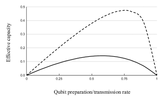
Figure 4: Capacity vs $\lambda$ for $\kappa=1$ (solid) and $\kappa=0.1$ (dotted).

In Fig. 4, the capacity expression in Theorem 5 is plotted against $\lambda$ for $\kappa=1$ and $\kappa=0.1$. Intuitively, the best $\lambda$ for a given $\kappa$ is the point where the curve reaches its peak.

Clearly, the optimal $\lambda$ is not close to $\mu$ ($=1$). Moreover, for $\lambda$ close $\mu$, the capacity is almost zero. This is because very high $\lambda$ leads to large waiting times for qubits and thus results in significant decoherence. Furthermore, the optimal $\lambda$ depends on $\kappa$ and hence, on the physical parameters of the buffer. The idealized i.i.d. setting fails to capture this crucial dependence.

4.4 Optimal queuing distributions

The effective capacity in the presence of buffer decoherence is a function of the stationary distribution of waiting times. Thus, in turn, it is heavily influenced by the time between preparation of two qubits and the time to process (transmit and receive) a qubit. A quantitative understanding of this dependence is useful for designing quantum communication systems.

In this section, we take a short stride in that direction by characterizing the optimal distributions in two queuing settings of general interest when the channel and buffer decoherence follows the exponential model in Eq. 50. The exponential decoherence model is physically the most well motivated model for capturing decoherence in terms of the interaction time with the environment.

First, we obtain a simpler expression of the capacity result in Theorem 5 for the exponential decoherence model.

Corollary 6.

The effective capacity in the presence of buffer decoherence is given by

$$\frac{\lambda}{\ln{2}}\sum_{k=1}^{\infty}\frac{1}{2k~{}(2k-1)}\mathbb{E}_{W\sim\pi}\left[\exp\left(-\kappa~{}k~{}W\right)\right],$$

when $p_{\mbox{\em eff}}(W)~{}=~{}1~{}-~{}\exp(-\kappa~{}W)$ for some $\kappa>0$.

Proof.

For the exponential decoherence model, the capacity expression in Theorem 5 becomes

$$\lambda~{}\mathbf{E}_{\pi}\left[1~{}-~{}h\left(\frac{1-\exp\left(-\frac{1}{2}\kappa~{}W\right)}{2}\right)\right].$$

The rest follows using the series expansion of $\log(1+x)$ for $|x|<1$ and algebraic manipulations. ∎

Note that the expression in Cor. 6 is valid for any stable queue, irrespective of the queuing discipline and distributions.

In the queuing literature, M/G/1 and G/M/1 are two popular classes of queuing models. In our setting, M/G/1 is equivalent to exponentially distributed (memoryless) preparation times and generally distributed processing or service times of qubits. G/M/1 is equivalent to generally distributed preparation times and exponentially distributed processing or service times. As a first step towards optimizing queuing distributions, one may ask: what are the best distribution for processing times and preparation times in M/G/1 and G/M/1 queues, respectively? The following theorems answer this question.

Theorem 7.

Among all quantum communication systems with M/G/1 buffering, symmetric GAD channel, and exponential decoherence, the system with deterministic processing or service time has the maximum effective capacity for any $\lambda$ and $\mu$ ($>\lambda$).

Proof.

Suppose there exists a service distribution for which $\mathbb{E}_{W\sim\pi}\left[\exp(-sW)\right]$ is more than any other service distribution with the same mean for any $s>0$. Then, from the capacity expression in Corollary 6, it is clear that under that particular distribution, each term in the series will be more the corresponding term for any other distribution. Hence, that distribution will achieve the maximum capacity among the class of all service distributions with the same mean.

Thus, to complete this proof, we need only to show that for exponentially distributed preparation times, the deterministic service time maximizes $\mathbb{E}_{W\sim\pi}\left[\exp(-sW)\right]$ for any $s>0$. This follows directly from the proof of Theorem 4 in [5]. ∎

Theorem 8.

Among all quantum communication systems with G/M/1 buffering, symmetric GAD channel, and exponential decoherence, the system with deterministic preparation/arrival time has the maximum effective capacity for any $\lambda$ and $\mu$ ($>\lambda$).

Proof.

Using the argument in the proof of Theorem 7, it is sufficient to show that for exponentially distributed service times, the deterministic preparation/arrival time maximizes $\mathbb{E}_{W\sim\pi}\left[\exp(-sW)\right]$ for any $s>0$.

The following two lemmas complete the proof of this theorem.

Lemma 9.

Among all arrival/preparation distributions with mean $\lambda^{-1}$ (>$\mu^{-1}$), $\mathbb{E}_{W\sim\pi}\left[\exp(-sW)\right]$ for any $s>0$ is maximized by that arrival/preparation distribution for which the solution to the G/M/1 fixed point equation

$$\sigma=\mathbb{E}_{A}\left[\exp\left(-(\mu-\mu~{}\sigma)~{}A\right)\right]$$

is the smallest.

Lemma 10.

Among all arrival/preparation distributions with mean $\lambda^{-1}$ (>$\mu^{-1}$), the solution to the G/M/1 fixed point equation

$$\sigma=\mathbb{E}_{A}\left[\exp\left(-(\mu-\mu~{}\sigma)~{}A\right)\right]$$

is the smallest for the deterministic arrival/preparation time $\lambda^{-1}$.

∎

Proof of Lemma 9.

The waiting time in a G/M/1 queue is exponentially distributed with mean $\frac{1}{\mu(1-\sigma)}$, where $\sigma$ is the solution to the fixed point equation

$$\sigma=\mathbb{E}_{A}\left[\exp\left(-(\mu-\mu~{}\sigma)~{}A\right)\right].$$

For exponentially distributed $W$, $\mathbb{E}\left[\exp(-sW)\right]$ decreases with $\mathbb{E}[W]$. Hence, for a given $\mu$, $\mathbb{E}\left[\exp(-sW)\right]$ increases as $\sigma$ decreases, which, in turn, implies Lemma 9. ∎

Proof of Lemma 10 is similar to the proof of Proposition 2 in [24].

5 Discussion and Conclusion

Understanding the classical capacity of a quantum channel and the means by which it can be achieved are fundamental, long-standing open issues in quantum information. In Sec. 3, we studied these issues for the generalized amplitude damping channel (GADC) ${\mathcal{A}}_{p,n}$, whose two parameters $p$ and $n$ represent the amount of damping and mixing, respectively. In Theorem 1, we found that for all $p$ and $n=1/2$, the Shannon capacity $C_{\rm Shan}$ of the (GADC) equals both its product state capacity $\chi^{(1)}$ and classical capacity $\chi$. In general, entanglement is required to achieve a channel’s classical capacity $\chi$. Interestingly, and of practical importance, our result implies that for the $n=1/2$ GADC, this capacity can be achieved without using any entanglement for encoding or decoding classical information into the channel. Entangled encoding is not required when $\chi^{(1)}$ is additive. Additivity is known to hold for some values of $p,n$ of the GADC, and also known for a variety of other channels.

Except for the $n=1/2$ GADC solved here, for most channels with additive $\chi^{(1)}$, finding the precise decoding that achieves capacity and certifying whether the decoding requires entanglement or not, remain open problems. For our solution of the $n=1/2$ GADC, in Sec. 3.2, we constructed several families of product encoding and decoding, including one that achieves capacity. Our solution opens an interesting possibility. Using a product encoding and product decoding more advanced than the ones discussed in Sec. 3.2 it may be possible to find an induced channel $M_{2}^{\prime}$, with capacity $C(M_{2}^{\prime})=C_{\rm Shan}({\mathcal{A}}_{p,n})=\chi^{(1)}({\mathcal{A}}_{p,n})$ for all $p,n$ where $\chi^{(1)}$ is additive. On the other hand, it could happen that even when $\chi^{(1)}({\mathcal{A}}_{p,n})$ is additive and no entanglement is required at the encoder, one requires entanglement at the decoder and $C_{\rm Shan}({\mathcal{A}}_{p,n})<\chi^{(1)}({\mathcal{A}}_{p,n})$. Which of these possibilities is true remains an open-problem. To completely resolve these open problems, one would first need to find all $p,n$ where $\chi^{(1)}({\mathcal{A}}_{p,n})$ is additive, a problem that also remains open.

Insights obtained from pursuing these open problems have the potential to not only enrich the i.i.d setting with point-to-point quantum channels but also provide a path to study non-i.i.d queue channel settings that arise in quantum networks. Another challenging avenue for future work is to characterise the queue channel capacity when the underlying noise model is not additive, as could be the case for certain parameter ranges of the GADC. This may require a fundamentally new approach to study quantum communication networks.

References

- [1] Wojciech Kozlowski, Axel Dahlberg, and Stephanie Wehner. Designing a quantum network protocol. In Proceedings of the 16th International Conference on Emerging Networking EXperiments and Technologies, CoNEXT ’20, page 1–16, New York, NY, USA, 2020. Association for Computing Machinery. doi:10.1145/3386367.3431293.
- [2] Kae Nemoto, Michael Trupke, Simon J Devitt, Burkhard Scharfenberger, Kathrin Buczak, Jörg Schmiedmayer, and William J Munro. Photonic quantum networks formed from nv- centers. Scientific reports, 6(1):1–12, 2016.
- [3] F Rozpędek, K Goodenough, J Ribeiro, N Kalb, V Caprara Vivoli, A Reiserer, R Hanson, S Wehner, and D Elkouss. Parameter regimes for a single sequential quantum repeater. Quantum Science and Technology, 3(3):034002, apr 2018. doi:10.1088/2058-9565/aab31b.
- [4] E. Shchukin, F. Schmidt, and P. van Loock. Waiting time in quantum repeaters with probabilistic entanglement swapping. Phys. Rev. A, 100:032322, Sep 2019. doi:10.1103/PhysRevA.100.032322.
- [5] P. Mandayam, K. Jagannathan, and A. Chatterjee. The classical capacity of additive quantum queue-channels. IEEE Journal on Selected Areas in Information Theory, 1(2):432–444, Aug 2020. doi:10.1109/JSAIT.2020.3015055.
- [6] Jeffrey H Shapiro. The quantum theory of optical communications. IEEE Journal of Selected Topics in Quantum Electronics, 15(6):1547–1569, 2009.
- [7] Sumeet Khatri, Kunal Sharma, and Mark M. Wilde. Information-theoretic aspects of the generalized amplitude-damping channel. Phys. Rev. A, 102:012401, Jul 2020. doi:10.1103/PhysRevA.102.012401.
- [8] H. Yuen and J. Shapiro. Optical communication with two-photon coherent states–part i: Quantum-state propagation and quantum-noise. IEEE Transactions on Information Theory, 24(6):657–668, 1978. doi:10.1109/TIT.1978.1055958.
- [9] Jeffrey H. Shapiro. The quantum theory of optical communications. IEEE Journal of Selected Topics in Quantum Electronics, 15(6):1547–1569, 2009. doi:10.1109/JSTQE.2009.2024959.
- [10] Wen-Jie Zou, Yu-Huai Li, Shu-Chao Wang, Yuan Cao, Ji-Gang Ren, Juan Yin, Cheng-Zhi Peng, Xiang-Bin Wang, and Jian-Wei Pan. Protecting entanglement from finite-temperature thermal noise via weak measurement and quantum measurement reversal. Phys. Rev. A, 95:042342, Apr 2017. doi:10.1103/PhysRevA.95.042342.
- [11] F Rozpędek, K Goodenough, J Ribeiro, N Kalb, V Caprara Vivoli, A Reiserer, R Hanson, S Wehner, and D Elkouss. Parameter regimes for a single sequential quantum repeater. Quantum Science and Technology, 3(3):034002, Apr 2018. doi:10.1088/2058-9565/aab31b.
- [12] Isaac L.Chuang and M. A. Nielsen. Prescription for experimental determination of the dynamics of a quantum black box. Journal of Modern Optics, 44(11-12):2455–2467, 1997. doi:10.1080/09500349708231894.
- [13] C. J. Myatt, B. E. King, Q. A. Turchette, C. A. Sackett, D. Kielpinski, W. M. Itano, C. Monroe, and D. J. Wineland. Decoherence of quantum superpositions through coupling to engineered reservoirs. Nature, 403(6767):269–273, Jan 2000. doi:10.1038/35002001.
- [14] Q. A. Turchette, C. J. Myatt, B. E. King, C. A. Sackett, D. Kielpinski, W. M. Itano, C. Monroe, and D. J. Wineland. Decoherence and decay of motional quantum states of a trapped atom coupled to engineered reservoirs. Phys. Rev. A, 62:053807, Oct 2000. doi:10.1103/PhysRevA.62.053807.
- [15] Luca Chirolli and Guido Burkard. Decoherence in solid-state qubits. Advances in Physics, 57(3):225–285, 2008. doi:10.1080/00018730802218067.
- [16] Hou Li-Zhen and Fang Mao-Fa. The holevo capacity of a generalized amplitude-damping channel. Chinese Physics, 16(7):1843–1847, jul 2007. doi:10.1088/1009-1963/16/7/006.
- [17] John Cortese. Relative entropy and single qubit holevo-schumacher-westmoreland channel capacity. arXiv e-prints, pages quant–ph/0207128, July 2002, quant-ph/0207128.
- [18] Dominic W. Berry. Qubit channels that achieve capacity with two states. Phys. Rev. A, 71:032334, Mar 2005. doi:10.1103/PhysRevA.71.032334.
- [19] Mark M. Wilde. Quantum Information Theory. Cambridge University Press, 2 edition, 2017. doi:10.1017/9781316809976.
- [20] A. S. Holevo. Index, pages 346–350. De Gruyter, 2012. doi:doi:10.1515/9783110273403.346.
- [21] Filippo Caruso, Vittorio Giovannetti, Cosmo Lupo, and Stefano Mancini. Quantum channels and memory effects. Reviews of Modern Physics, 86(4):1203, 2014.
- [22] Masahito Hayashi and Hiroshi Nagaoka. General formulas for capacity of classical-quantum channels. IEEE Transactions on Information Theory, 49(7):1753–1768, 2003.
- [23] Krishna Jagannathan, Avhishek Chatterjee, and Prabha Mandayam. Qubits through queues: The capacity of channels with waiting time dependent errors. In 2019 National Conference on Communications (NCC), pages 1–6. IEEE, 2019.
- [24] Avhishek Chatterjee, Daewon Seo, and Lav R Varshney. Capacity of systems with queue-length dependent service quality. IEEE Transactions on Information Theory, 63(6):3950–3963, 2017.
- [25] Wenhan Dai, Tianyi Peng, and Moe Z Win. Quantum queuing delay. IEEE Journal on Selected Areas in Communications, 38(3):605–618, 2020.
- [26] Mihir Pant, Hari Krovi, Don Towsley, Leandros Tassiulas, Liang Jiang, Prithwish Basu, Dirk Englund, and Saikat Guha. Routing entanglement in the quantum internet. npj Quantum Information, 5(1):1–9, 2019.
- [27] Gayane Vardoyan, Saikat Guha, Philippe Nain, and Don Towsley. On the stochastic analysis of a quantum entanglement distribution switch. IEEE Transactions on Quantum Engineering, 2:1–16, 2021. doi:10.1109/TQE.2021.3058058.
- [28] S. Arimoto. An algorithm for computing the capacity of arbitrary discrete memoryless channels. IEEE Transactions on Information Theory, 18(1):14–20, 1972. doi:10.1109/TIT.1972.1054753.
- [29] R. Blahut. Computation of channel capacity and rate-distortion functions. IEEE Transactions on Information Theory, 18(4):460–473, 1972. doi:10.1109/TIT.1972.1054855.
- [30] A. S. Holevo. The capacity of the quantum channel with general signal states. IEEE Transactions on Information Theory, 44(1):269–273, Jan 1998. doi:10.1109/18.651037.
- [31] Benjamin Schumacher and Michael D. Westmoreland. Sending classical information via noisy quantum channels. Phys. Rev. A, 56:131–138, Jul 1997. doi:10.1103/PhysRevA.56.131.
- [32] Masahide Sasaki, Stephen M. Barnett, Richard Jozsa, Masao Osaki, and Osamu Hirota. Accessible information and optimal strategies for real symmetrical quantum sources. Phys. Rev. A, 59:3325–3335, May 1999. doi:10.1103/PhysRevA.59.3325.
- [33] P. W. Shor. The adaptive classical capacity of a quantum channel, or information capacities of three symmetric pure states in three dimensions. IBM Journal of Research and Development, 48(1):115–137, 2004. doi:10.1147/rd.481.0115.
- [34] C. H. Bennett and P. W. Shor. Quantum information theory. IEEE Transactions on Information Theory, 44(6):2724–2742, Oct 1998. doi:10.1109/18.720553.
- [35] M. B. Hastings. Superadditivity of communication capacity using entangled inputs. Nat Phys, 5(4):255–257, Apr 2009. doi:10.1038/nphys1224.
- [36] Christopher King. Additivity for unital qubit channels. Journal of Mathematical Physics, 43(10):4641–4653, 2002. doi:10.1063/1.1500791.
- [37] C. King. The capacity of the quantum depolarizing channel. IEEE Transactions on Information Theory, 49(1):221–229, Jan 2003. doi:10.1109/TIT.2002.806153.
- [38] Christopher King, Keiji Matsumoto, Michael Nathanson, and Mary Beth Ruskai. Properties of conjugate channels with applications to additivity and multiplicativity. Markov Process and Related Fields, 13:391–423, 2007. http://math-mprf.org/journal/articles/id1123/.
- [39] Peter W. Shor. Additivity of the classical capacity of entanglement-breaking quantum channels. Journal of Mathematical Physics, 43(9):4334–4340, 2002. doi:10.1063/1.1498000.
- [40] T. S. Han. Information-spectrum Methods in Information Theory. Springer-Verlag Berlin Heidelberg, 2003.
- [41] Sergio Verdú and T. S. Han. A general formula for channel capacity. IEEE Transactions on Information Theory, 40(4):1147–1157, 1994.
- [42] Carl W. Helstrom. Quantum detection and estimation theory. Journal of Statistical Physics, 1(2):231–252, Jun 1969. doi:10.1007/BF01007479.
- [43] Michael A. Nielsen and Isaac L. Chuang. Quantum Computation and Quantum Information: 10th Anniversary Edition. Cambridge University Press, New York, NY, USA, 10th edition, 2011.