Task-Specific Normalization for Continual Learning of Blind Image Quality Models

Abstract

The computational vision community has recently paid attention to continual learning for blind image quality assessment (BIQA). The primary challenge is to combat catastrophic forgetting of previously-seen IQA datasets (i.e., tasks). In this paper, we present a simple yet effective continual learning method for BIQA with improved quality prediction accuracy, plasticity-stability trade-off, and task-order/-length robustness. The key step in our approach is to freeze all convolution filters of a pre-trained deep neural network (DNN) for an explicit promise of stability, and learn task-specific normalization parameters for plasticity. We assign each new task a prediction head, and load the corresponding normalization parameters to produce a quality score. The final quality estimate is computed by a weighted summation of predictions from all heads with a lightweight $K$-means gating mechanism, without leveraging the test-time oracle. Extensive experiments on six IQA datasets demonstrate the advantages of the proposed method in comparison to previous training techniques for BIQA.

I Introduction

There is an emerging trend to develop image quality assessment (IQA) models [1] and image processing methods in an alternating manner: better IQA models provide more reliable guidance to the design and optimization of the latter, while new image processing algorithms call for the former to handle novel visual artifacts. This suggests a desirable IQA model to easily adapt to such distortions by continually learning from new data (see Fig. 1).

This paper focuses on continual learning of blind IQA (BIQA) models [2, 3], which predict the perceptual quality of a “distorted” image without reference to an original undistorted image. Over the past $20$ years, the research in BIQA has shifted from handling distortion-specific [4], single-stage [5], synthetic artifacts to general-purpose [6], multi-stage [7], authentic ones, and from relying on handcrafted features to purely data-driven approaches [8]. Existing BIQA models are generally developed and tested using human-rated images from the same dataset, i.e., within the same subpopulation [2]. As such, even the best-performing BIQA methods, e.g., those based on deep neural networks (DNNs) are bound to encounter subpopulation shift when deployed in the real world.

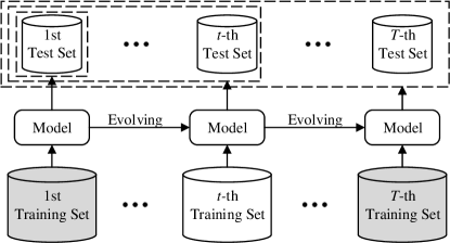
Figure 1: Illustration of continual learning for BIQA. The grey cylinders denote the inaccessibility of previous and future training data. During testing, we use all previous and the current test sets to evaluate the stability and plasticity of the learned BIQA model.

Direct fine-tuning model parameters with new data may result in catastrophic forgetting [9, 10] of previously-seen data. The dataset combination trick in [11] has been proven effective in handling subpopulation shift, but is limited by the computational scalability and the dataset accessibility. Recently, Zhang et al. [2] formulated continual learning for BIQA with five desiderata. Meanwhile, they described the first continual learning method of training BIQA models based on a technique called learning with forgetting (LwF) [12]. Like many continual learning methods (for classification), LwF adds a form of regularization [13] to mildly adjust model parameters for new tasks while respecting old tasks. Nevertheless, this type of regularization-based methods have two limitations. First, it is practically difficult to set the trade-off parameter for stability (i.e., the ability to consolidate acquired knowledge from old tasks) and plasticity (i.e., the ability to learn new knowledge from the current task). Second, the performance is usually sensitive to the order and the length of the task sequence [14, 2].

In this paper, we describe a simple yet effective continual learning method for BIQA based on parameter decomposition. Specifically, we start with a pre-trained DNN as the feature extractor. We freeze all convolution filters, and share them along with all parameter-free nonlinear activation and pooling layers across tasks during the entire continual learning process. We append a prediction head, implemented by a fully connected (FC) layer, when learning a new task. We allow the parameters of batch normalization (BN) [15] following each convolution to be specifically learned for each task. Through this task-specific normalization, a better plasticity-stability trade-off can be made with a negligible increase in model size. During inference, we load each group of BN parameters to produce a quality estimate using the corresponding prediction head. The final quality score is computed by a weighted summation of predictions from all heads with a lightweight $K$-means gating (KG) mechanism.

In summary, our contributions are threefold.

• We propose a new continual learning method for BIQA. Our resulting method, which we name TSN-IQA, can integrate new knowledge into BN parameters without catastrophic forgetting of acquired knowledge.

• We design a lightweight KG module that only requires learning a set of distortion-aware BN parameters (rather than relying on an extra DNN [2]) to compute the weightings of prediction heads during inference.

• We perform extensive experiments to demonstrate the advantages of our method in terms of quality prediction accuracy, plasticity-stability trade-off, and task-order/-length robustness.

II Related Work

In this section, we give an overview of recent progress in BIQA, especially on handling subpopulation shift. We then review representative continual learning methods for classification, and discuss normalization techniques in the broader context of deep learning.

II-A BIQA Models

Many early BIQA methods are based on hand-engineered natural scene statistics (NSS) in spatial [6, 16], transformed [17], or both domains [18]. In recent years, deep learning began to show its promise in the field of BIQA. Patchwise training [19, 8], transfer learning [20], and quality-aware pre-training [21, 22, 23] were proposed to compensate for the lack of human-rated data. Of particular interest is the introduction of IQA datasets with realistic distortions [24, 25, 26], which excites a series of BIQA models to address the synthetic-to-real generalization. Zhang et al. [27] assembled two network branches to account for synthetic and realistic distortions separately. Su et al. [28] investigated content-aware convolution for robust BIQA, while Zhu et al. [29] aimed to learn more transferable quality-aware representations by meta-learning. Zhang et al. [11] proposed a dataset combination strategy to train BIQA models on multiple IQA datasets. They later formulated the continual learning setting for BIQA as a new paradigm, and introduced a method that combines LwF [12] with a K-means gating (KG) module [2]. Concurrently, Liu et al. [3] proposed a continual learning method for BIQA based on a replay strategy. Ma et al. [30, 31] proposed a remember-and-reuse network that utilizes a pruning technique to enable continual learning of BIQA models. In this paper, we follow the setting of [2], and propose a new continual learning method for BIQA with significantly improved performance in several aspects.

II-B Continual Learning for Classification

While humans rarely forget previously-learned knowledge catastrophically, machine learning models such as DNNs tend to completely forget old concepts when learning new ones [32, 10]. Enforcing regularization is a common practice to mitigate the catastrophic forgetting problem in continual learning. For example, Li and Hoiem [12] proposed LwF, which leverages model predictions of previous tasks as pseudo labels. Elastic weight consolidation (EWC) [33], variational continual learning (VCL) [34], synaptic intelligence (SI) [35], and memory-aware synapses (MAS) [36] work similarly by identifying and penalizing changes to important parameters of previous tasks. From this perspective, parameter decomposition [13] can be seen as a form of hard regularization, disentangling model parameters into task-agnostic and task-specific groups. This may be done by either masking learned parameters of previous tasks [37, 38, 39] or growing new branches to accommodate new tasks [40]. For example, Yoon et al. [14] proposed additive parameter decomposition to achieve task-order robustness. Singh et al.[41] calibrated the convolution responses of a continually trained DNN with a few parameters for new tasks. In this paper, we take a similar but much simpler parameter decomposition approach to achieve accurate and robust continual learning for BIQA. More importantly, our method does not rely on the task oracle during inference, which is in stark contrast to continual learning methods for classification.

II-C Normalization in Deep Learning

There is increasing evidence that normalization is a canonical neural computation throughout the visual system, and in many other sensory modalities and brain regions [42]. As biologically inspired, deep learning also incorporates different instantiations of normalization for various purposes, such as accelerating model training [15] and improving model generalization [43]. BN is a de-facto technique to improve the training efficiency of DNNs, in which the convolution responses are divided by the standard deviation (std) of a pool of responses along the batch (and spatial) dimensions. Xie et al. [44] learned separate BN layers to harness adversarial examples, which improves image recognition models. Li et al. [45] proposed adaptive BN for domain adaptation, assuming that domain-invariant and domain-specific computations are learned by the convolution filters and the BN layers, respectively. Chang et al. [46] specialized BN layers using a two-stage algorithm for unsupervised domain adaptation. Dumoulin et al. [47] relied on conditional instance normalization [48] to synthesize the artistic styles of diverse paintings. Zhang et al. [49] presented a passport normalization for deep model intellectual property protection against infringement threats. Recently, Pham et al.[50] proposed a continual normalization method to mitigate the catastrophic forgetting problem in online learning. In this paper, we introduce task-specific BN to accomplish continual learning of DNN-based BIQA models.

III Proposed Method

In this section, we first revisit the formulation of continual learning for BIQA in [2], and then elaborate the training and inference procedures of the proposed TSN-IQA. To facilitate mathematical comprehension, we summarize a list of variables in Table I.

III-A Problem Formulation

When training on the $t$-th dataset $\mathcal{D}_{t}$, i.e., the $t$-th task, a BIQA model $f_{w}$, parameterized by a vector $w$, has no direct access to previous training images in $\{\mathcal{D}_{k}\}_{k=1}^{t-1}$, leading to the following objective:

$$\mathcal{L}(\mathcal{D}_{t};w)=\frac{1}{|\mathcal{D}_{t}|}\sum_{(x,q)\in\mathcal{D}_{t}}\ell(f_{w}(x),q)+\lambda r(w),$$ (1)

where $x$ and $q$ denote the “distorted” image and the corresponding mean opinion score (MOS), respectively. $\ell(\cdot)$ is a quantitative measure of quality prediction performance, and $r(\cdot)$ is an optional regularizer. A good BIQA model under this setting should adapt well to new tasks, and meanwhile endeavor to mitigate catastrophic forgetting of old tasks as measured by

$$\sum_{k=1}^{t}\mathcal{L}(\mathcal{V}_{k};w)=\sum_{k=1}^{t}\left(\frac{1}{|\mathcal{V}_{k}|}\sum_{(x,q)\in\mathcal{V}_{k}}\ell(f_{w}(x),q)\right),$$ (2)

where $\mathcal{V}_{k}$ denotes the test set for the $k$-th task. Five desiderata are suggested in [2] to make continual learning for BIQA feasible and nontrivial: 1) common perceptual scale, 2) robust to subpopulation shift, 3) limited access to previous data, 4) no test-time oracle, and 5) bounded memory footprint.

TABLE I: List of variables

Notation	Description
$(x,y)$	an image pair
$(\mu_{x}$, $\mu_{y})$	MOSs of $x$ and $y$
$\mathcal{D}_{t}$	the $t$-th dataset
$\mathcal{P}_{t}$	the $t$-th paired dataset
$N_{t}$	# of image pairs in the $t$-th paired dataset
$f_{\phi}$	a DNN parameterized by a vector $\phi$
$h_{\psi_{t}}$	the $t$-th prediction head parameterized by $\psi_{t}$
$r(x,y)$	the binary quality label of $(x,y)$
$\hat{p}_{t}(x,y)$	the predicted probability of $(x,y)$ for the $t$-th task
$(\mu_{t},\sigma_{t},\gamma_{t},\beta_{t})$	the 4-tuple BN parameters for the $t$-th task
$c_{kst}$	the $k$-th centroid at the $s$-th stage for the $t$-th task
$d_{st}(x)$	the perceptual relevance of $x$ to the $t$-th task
$a_{st}(x)$	the weighting of $x$ for the $t$-th prediction head
$\hat{q}(x)$	the predicted quality score of $x$

III-B Model Estimation

Inspired by UNIQUE [11], we exploit relative quality information to learn a common perceptual scale for all tasks. Specifically, given an image pair $(x,y)$, we compute a binary label:

$$r(x,y)=\begin{cases}1&\mbox{if }\mu_{x}\geq\mu_{y}\\ 0&\mbox{otherwise}\end{cases},$$ (3)

where $\mu_{x}$ and $\mu_{y}$ are the MOSs of $x$ and $y$, respectively. Careful readers may find that we do not infer a continuous value $p(x,y)$, which denotes the probability of $x$ perceived better than $y$ based on the Thurstone’s model [51] or the Bradley-Terry model [52] as typically done in previous work [23, 11]. This is because the computed probability may vary with the precision of the subjective testing methodology. For example, if $x$ is marginally better than $y$ and a precise subjective method such as the two-alternative forced choice (2AFC) is adopted, $p(x,y)$ can be close to one. By contrast, if a less precise subjective method such as the single stimulus continuous quality rating is used, $p(x,y)$ may only be slightly larger than $0.5$. Compared to $p(x,y)$, we also empirically observe that $r(x,y)$ leads to faster convergence and improved accuracy results. In summary, when learning the $t$-th task, we transform $\mathcal{D}_{t}=\{x^{(i)}_{t},\mu^{(i)}_{t}\}_{i=1}^{|\mathcal{D}_{t}|}$ to $\mathcal{P}_{t}=\{(x^{(i)}_{t},y^{(i)}_{t}),r^{(i)}_{t}\}_{i=1}^{N_{t}}$, where $N_{t}\leq\binom{|\mathcal{D}_{t}|}{2}$.

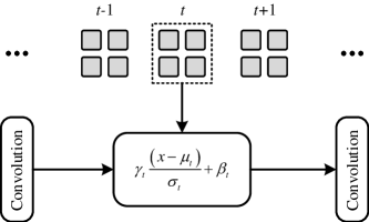
Figure 2: Illustration of task-specific BN. The parameters of all convolutions are frozen and shared across all tasks. A group of BN parameters is customized for each task.

Our BIQA model consists of a feature extractor implemented by a DNN, $f_{\phi}(\cdot)$, producing a fixed-length image representation independent of input resolution. For the $t$-th task, we append a prediction head implemented by an FC layer, $h_{\psi_{t}}(\cdot)$, outputting a corresponding quality score. Under the Thurstone’s Case V model [51], we estimate the probability that $x$ is of higher quality than $y$ by

$$\hat{p}_{t}(x,y)=\Phi\left(\frac{h_{\psi_{t}}(f_{\phi}(x))-h_{\psi_{t}}(f_{\phi}(y))}{\sqrt{2}}\right),$$ (4)

where the quality prediction variance is fixed to one. We measure the statistical distance between the ground-truth labels and predicted probabilities using the fidelity loss [53] due to its favorable optimization behaviors [11]:

$$\ell(x,y;\phi,\psi_{t})=1 -\sqrt{r(x,y)\hat{p}_{t}(x,y)}$$

$$-\sqrt{(1-r(x,y))(1-\hat{p}_{t}(x,y))}.$$ (5)

To make a better trade-off between plasticity and stability while keeping a bounded model size, our BIQA method chooses to maximally share computation across tasks, and customize a tiny fraction of parameters to account for the incremental difference introduced by new tasks. In particular, our feature extractor is composed of several stages of convolution, BN, halfwave-rectification (i.e., ReLU nonlinearity), and max-pooling. We freeze all pre-trained convolution parameters during model development, and learn a group of $4$-tuple BN parameters for the $t$-th task

$$z_{\mathrm{BN}}=\gamma_{t}\left(\frac{z-\mu_{t}}{\sigma_{t}}\right)+\beta_{t},$$ (6)

where $\mu_{t}$ and $\sigma_{t}$ are the mean and the std estimated by the exponentially decaying moving average over mini-batches. $\gamma_{t}$ and $\beta_{t}$ are the learnable scale and shift parameters (see also Fig. 2). After training on a $T$-length task sequence, we obtain $T$ groups of task-specific BN parameters.

III-C Model Inference

During inference, we successively load each of $T$ groups of BN parameters along with the corresponding FC layer to compute $T$ quality scores. Due to the unavailability of the task oracle, we rely on an improved KG module [2] with a lightweight design goal, which is made possible by the proposed parameter decomposition scheme. Unlike [2], we only train a set of task-agnostic BN parameters on a large-scale image set with various synthetic distortions [27] for distortion-aware weighting computation, while keeping all convolution filters intact. Since the original BN parameters of the pre-trained feature extractor are not necessary, our gating mechanism introduces essentially no extra parameters, and adheres to the desideratum of bounded memory footprint.

We present the overview of the inference process in Fig. 3. During learning the $t$-th task, we load the distortion-aware BN parameters to the pre-trained $f_{\phi}$ to compute globally pooled convolution responses of image $x$ at the $s$-th stage, $\bar{f}_{\phi_{s}}(x)$. Given $S$-stage convolutions, we obtain a feature summary of $\mathcal{D}_{t}$: $\{\bar{f}_{\phi_{1}}(x_{t}^{(i)}),\ldots,\bar{f}_{\phi_{S}}(x_{t}^{(i)})\}_{i=1}^{|\mathcal{D}_{t}|}$. We then apply $K$-means [54] (for each stage of convolution responses) to compute $S$ groups of $K$ centroids $\{\{c_{kst}\}_{k=1}^{K}\}_{s=1}^{S}$.

We measure the perceptual relevance of $x$ to $\mathcal{D}_{t}$ by computing the minimal Euclidean distances between $\bar{f}_{\phi_{s}}(x)$ and $\{c_{kst}\}_{k=1}^{K}$:

$$d_{st}(x)=\min_{k}\|\bar{f}_{\phi_{s}}(x)-c_{kst}\|_{2}\,.$$ (7)

We pass $\{d_{st}(x)\}_{t=1}^{T}$ to a softmin function to compute the weightings at the $s$-th stage for the $t$-th prediction head:

$$a_{st}(x)=\frac{{\rm exp}(-{\tau}d_{st}(x))}{\sum_{t=1}^{T}{\rm exp}(-{\tau}d_{st}(x))},$$ (8)

where $\tau\geq 0$ is a parameter to control the smoothness of the softmin function. We further average the weightings across stages to obtain

$$a_{t}(x)=\frac{1}{S}\sum_{s}a_{st}(x).$$ (9)

We last compute the overall quality score by the inner product between the weighting and quality prediction vectors:

$$\hat{q}(x)=\sum_{t=1}^{T}a_{t}(x)h_{\psi_{t}}(f_{\phi}(x)).$$ (10)

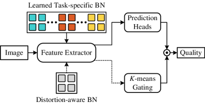
Figure 3: Overview of the inference process. The solid line indicates the pipeline of loading task-specific BN parameters learned for different tasks (denoted by different colors) and making the quality prediction using the corresponding prediction heads. The dotted line indicates the process of loading distortion-aware BN parameters and computing weightings for all prediction heads with the KG module.

IV Experiments

In this section, we first describe the experimental setup for continual learning of BIQA models, and then compare the proposed TSN-IQA against previous training techniques, supplemented by abundant ablation studies. The source code will be made publicly available at https://github.com/zwx8981 to facilitate reproducible research.

TABLE II: Summary of IQA datasets used in our experiments. CLIVE stands for the LIVE Challenge Database. TID2013 [55] and SPAQ [56] are used for cross-database evaluation. SS: Single stimulus. DS: Double stimulus. MS: Multiple stimulus. CQR: Continuous quality rating. ACR: Absolute category rating. CS: Crowdsourcing. PC: Paired Comparison

Dataset	# of Images	# of Training Pairs	# of Test Images	Scenario	# of Types	Testing Methodology	Year
LIVE [5]	779	7,780	163	Synthetic	5	SS-CQR	2006
CSIQ [57]	866	8,786	173	Synthetic	6	MS-CQR	2010
BID [24]	586	11,204	117	Realistic	N.A.	SS-CQR	2011
CLIVE [25]	1,162	24,604	232	Realistic	N.A.	SS-CQR-CS	2016
KonIQ-10K [26]	10,073	139,274	2,015	Realistic	N.A.	SS-ACR-CS	2018
KADID-10K [58]	10,125	140,071	2,000	Synthetic	25	DS-ACR-CS	2019
TID2013 [55]	3,000	N.A.	3,000	Synthetic	25	DS-PC	2013
SPAQ [56]	11,125	N.A.	11,125	Realistic	N.A.	SS-CQR	2020

TABLE III: Performance comparison in terms of $\mathrm{mSRCC}$, $\mathrm{mPI}$, $\mathrm{mSI}$, and $\mathrm{mPSI}$. Task-aware and task-agnostic evaluation settings correspond to quality prediction with and without the task oracle, respectively. All methods are trained in chronological order

Setting	Method	$\mathrm{mSRCC}$	$\mathrm{mPI}$	$\mathrm{mSI}$	$\mathrm{mPSI}$
Task-aware	SI-O	0.786	0.858	0.886	0.872
	MAS-O	0.779	0.853	0.882	0.868
	LwF-O	0.804	0.841	0.970	0.906
	TSN-IQA-O	0.855	0.855	1.000	0.928
Task-agnostic	SL	0.666	0.851	0.751	0.801
	SI	0.762	0.858	0.876	0.867
	SI-KG	0.778	0.856	0.877	0.867
	MAS	0.717	0.853	0.862	0.858
	MAS-KG	0.769	0.854	0.872	0.863
	LwF	0.691	0.841	0.890	0.866
	LwF-KG	0.801	0.837	0.963	0.900
	TSN-IQA	0.846	0.853	0.979	0.916

TABLE IV: Performance comparison in terms of SRCC between TSN-IQA and others. Best results in each section are highlighted in bold, and results of future tasks are marked in grey

Dataset	Method	LIVE [5]	CSIQ [57]	BID [24]	CLIVE [25]	KonIQ-10K [26]	KADID-10K [58]
All	JL	0.969	0.815	0.842	0.827	0.856	0.896
LIVE	SL	0.927	0.645	0.726	0.407	0.645	0.556
	LwF	0.927	0.645	0.726	0.407	0.645	0.556
	LwF-KG	0.927	0.645	0.726	0.407	0.645	0.556
	SI	0.927	0.645	0.726	0.407	0.645	0.556
	SI-KG	0.927	0.645	0.726	0.407	0.645	0.556
	MAS	0.927	0.645	0.726	0.407	0.645	0.556
	MAS-KG	0.927	0.645	0.726	0.407	0.645	0.556
	TSN-IQA	0.956	0.677	0.645	0.465	0.680	0.504
CSIQ	SL	0.903	0.846	0.656	0.426	0.628	0.552
	LwF	0.954	0.805	0.692	0.440	0.684	0.581
	LwF-KG	0.923	0.815	0.725	0.472	0.680	0.530
	SI	0.953	0.880	0.596	0.415	0.646	0.575
	SI-KG	0.940	0.874	0.596	0.414	0.643	0.554
	MAS	0.948	0.874	0.617	0.412	0.659	0.581
	MAS-KG	0.935	0.870	0.617	0.412	0.658	0.566
	TSN-IQA	0.950	0.850	0.672	0.477	0.696	0.522
BID	SL	0.716	0.569	0.766	0.660	0.645	0.374
	LwF	0.938	0.792	0.782	0.572	0.729	0.547
	LwF-KG	0.920	0.796	0.789	0.511	0.718	0.528
	SI	0.886	0.835	0.814	0.562	0.718	0.571
	SI-KG	0.885	0.839	0.813	0.536	0.717	0.570
	MAS	0.907	0.826	0.785	0.556	0.682	0.595
	MAS-KG	0.841	0.833	0.785	0.541	0.685	0.594
	TSN-IQA	0.952	0.855	0.812	0.720	0.701	0.494
CLIVE	SL	0.448	0.472	0.839	0.836	0.756	0.306
	LwF	0.814	0.646	0.820	0.802	0.774	0.522
	LwF-KG	0.910	0.776	0.785	0.776	0.756	0.552
	SI	0.925	0.792	0.804	0.809	0.804	0.536
	SI-KG	0.929	0.800	0.807	0.811	0.803	0.527
	MAS	0.911	0.759	0.818	0.821	0.776	0.497
	MAS-KG	0.928	0.770	0.828	0.821	0.774	0.496
	TSN-IQA	0.953	0.837	0.833	0.799	0.730	0.502
KonIQ-10K	SL	0.785	0.708	0.768	0.723	0.895	0.593
	LwF	0.868	0.705	0.768	0.725	0.889	0.598
	LwF-KG	0.913	0.741	0.800	0.779	0.870	0.617
	SI	0.850	0.708	0.781	0.713	0.888	0.608
	SI-KG	0.884	0.693	0.793	0.739	0.885	0.611
	MAS	0.901	0.712	0.775	0.693	0.883	0.613
	MAS-KG	0.936	0.716	0.797	0.737	0.880	0.620
	TSN-IQA	0.959	0.813	0.823	0.796	0.869	0.568
KADID-10K	SL	0.881	0.639	0.635	0.387	0.618	0.835
	LwF	0.853	0.736	0.676	0.418	0.622	0.842
	LwF-KG	0.888	0.731	0.766	0.741	0.831	0.849
	SI	0.895	0.761	0.740	0.612	0.731	0.832
	SI-KG	0.871	0.742	0.782	0.687	0.764	0.824
	MAS	0.876	0.744	0.753	0.419	0.677	0.831
	MAS-KG	0.857	0.758	0.808	0.600	0.752	0.840
	TSN-IQA	0.954	0.801	0.829	0.786	0.870	0.830

IV-A Experimental Setup

We select six widely used IQA datasets: LIVE [5], CSIQ [57], BID [24], LIVE Challenge [25], KonIQ-10K [26], and KADID-10K [58]. We summarize the details of the six datasets in Table II. In general, the number of training pairs is proportional to the number of images in the training set of each dataset. As previously discussed, the diversity of subjective testing methodologies among different datasets may result in varying MOS precision [59, 60], encouraging us to consider binary ground-truth labels in Eq. (3). Following [2], we organize these datasets in chronological order for the main experiments. We randomly sample $70\%$ and $10\%$ images from each dataset for training and validation, respectively, and leave the remaining for testing. To ensure content independence in LIVE, CSIQ, and KADID-10K, we divide the training and test sets according to the reference images.

We choose a variant of ResNet-18 [61] as the feature extractor. We keep the front convolution and four residual blocks, which are indexed by Stage $1$ to Stage $4$, respectively. We append an FC layer as the prediction head on top of the convolution response from Stage $4$, and compute the weightings (see Eq. (7)) using the convolution responses from later two stages. As such, $10,112$ learnable parameters are introduced by BN and FC layers for each new task, accounting for less than $0.18\%$ of the total network parameters. During inference, the number of centroids used in $K$-means is set to $K=128$ for each new task, which introduces $98,304$ parameters for additional memory budget, accounting for about $0.88\%$ of the backbone network parameters. Putting together, the current configuration ensures that TSN-IQA conforms to the bounded memory footprint desideratum.

For each task, stochastic optimization is carried out by Adam [62] with an initial learning rate of $1\times 10^{-3}$. We decay the learning rate by a factor of $10$ at the $8$-th epoch, and train our method for a maximum of twelve epochs. We set the temperature to $\tau=32$ in Eq. (8). We test on images of the original size.

As suggested in [2], we use Spearman’s rank correlation coefficient (SRCC) to measure the prediction performance. When continually learning a BIQA model on a $T$-length task sequence, we compute the mean SRCC between model predictions and MOSs of each dataset as a measure of prediction accuracy:

$$\mathrm{mSRCC}=\frac{1}{T}\sum_{k=1}^{T}\mathrm{SRCC}_{Tk},$$ (11)

where $\mathrm{SRCC}_{tk}$ is the SRCC result of the $t$-th model on the $k$-th dataset. We then compute a mean plasticity index ($\mathrm{mPI}$):

$$\mathrm{mPI}=\frac{1}{T}\sum_{t=1}^{T}\mathrm{PI}_{t}=\frac{1}{T}\sum_{t=1}^{T}\mathrm{SRCC}_{tt},$$ (12)

i.e., the average result of the model on the current dataset along the task sequence, and a mean stability index ($\mathrm{mSI}$) by measuring the variability of model performance on old data when learning on a new task:

$$\mathrm{mSI}=\frac{1}{T}\sum_{t=1}^{T}\mathrm{SI}_{t},$$ (13)

where

$$\mathrm{SI}_{t}=\begin{cases}1&t=1\\ \frac{1}{t-1}\sum_{k=1}^{t-1}\widehat{\mathrm{SRCC}}_{tk}&t>1\end{cases},$$ (14)

where $\widehat{\mathrm{SRCC}}_{tk}$ for $k<t$ is computed between the predictions of the $t$-th and $k$-th models. $\mathrm{mSRCC}$, $\mathrm{mPI}$, and $\mathrm{mSI}$ measure different and complementary aspects of a continually learned BIQA model. We also quantify the plasticity-stability trade-off using a mean plasticity-stability index ($\mathrm{mPSI}$) over a list of $T$ tasks:

$$\mathrm{mPSI}=\frac{1}{T}\sum_{t=1}^{T}\mathrm{PSI}_{t}=\frac{1}{2T}\sum_{t=1}^{T}\left(\mathrm{PI}_{t}+\mathrm{SI}_{t}\right).$$ (15)

IV-B Competing Methods

We describe several competing methods for training.

• Separate Learning (SL) is the standard in BIQA, which trains the model using a single prediction head on one of the six training sets.

• Joint Learning (JL) is a dataset combination trick [11] to address the cross-distortion-scenario challenge in BIQA. As an upper bound of all continual learning methods, JL trains the model with a single head on the combination of all six training sets.

• LwF [12] in BIQA is based on a multi-head architecture, which introduces a stability regularizer that uses the previous model outputs as soft labels to preserve the performance of previously-seen data. LwF relies on the newest head for quality prediction. We also leverage the task oracle to select the corresponding head for quality prediction, denoted by LwF-O.

• LwF-KG [2] uses a modified LwF [12] for training and the KG mechanism for inference. For a fair comparison, we use the same backbone network as in TSN-IQA to implement LwF-KG instead of the original two-stream network [2].

• SI [35] is also a regularization-based continual learning method, which estimates important parameters for previous tasks. Similar to LwF, we implement a multi-head architecture for SI, and rely on the newest head to predict image quality. We try to improve the performance with the KG mechanism, denoted by SI-KG, and leverage the task oracle as well, denoted by SI-O.

• MAS [35] shares a similar philosophy with SI to penalize the changes to important weights. The difference lies only in the calculation of the cumulative importance measure. Similarly, MAS uses the latest head for quality prediction, and has two variants that include the KG module and the task oracle, denoted by MAS-KG and MAS-O, respectively.

• TSN-IQA makes use of task-specific BN to handle new tasks, and enhances the KG module in [2] using rich feature hierarchies with less memory footprint. We also replace the KG module with the task oracle for quality prediction, denoted by TSN-IQA-O.

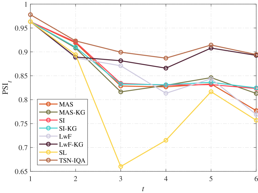
Figure 4: ${\mathrm{PSI}}_{t}$ as a function of the task index $t$.

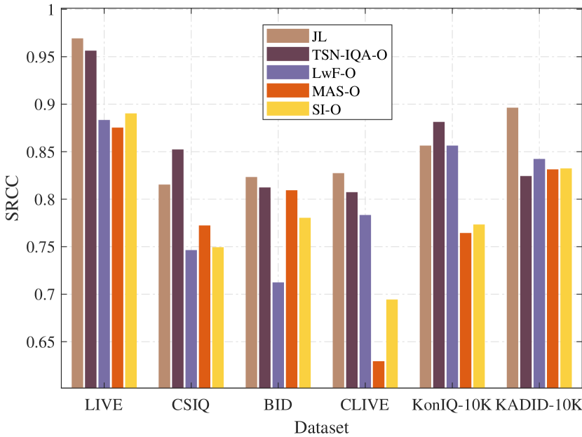
Figure 5: Performance comparison in terms of SRCC among models after finishing continual learning and when the test-time oracle is available.

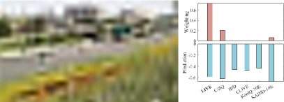
(a) $\hat{q}(x)=-0.599$

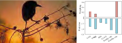
(b) $\hat{q}(x)=-0.480$

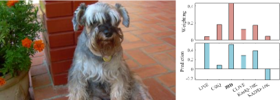
(c) ${\color[rgb]{0,0,0}\hat{q}(x)=0.353}$

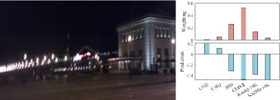
(d) ${\color[rgb]{0,0,0}\hat{q}(x)=-0.394}$

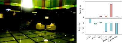
(e) ${\color[rgb]{0,0,0}\hat{q}(x)=-0.304}$

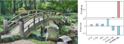
(f) ${\color[rgb]{0,0,0}\hat{q}(x)=-0.618}$

Figure 6: Learned common perceptual scale to embed images from the six IQA datasets. The bar charts of weightings and quality predictions are also presented alongside each image. The dataset in bold indicates the origin of the test image. The final quality prediction $\hat{q}(x)$ is shown in the subcaption. Zoom in for better distortion visibility.

IV-C Main Results

Table III lists $\mathrm{mSRCC}$, $\mathrm{mPI}$, $\mathrm{mSI}$, and $\mathrm{mPSI}$ results on the six IQA test sets. Several interesting observations have been made. First, without any remedy for catastrophic forgetting, the performance of SL is far from satisfactory, consistent with previous findings [2]. Particularly, we identify a significant performance drop when SL transits from CSIQ to BID (see Table IV), where an apparent subpopulation shift from synthetic to realistic distortions is introduced. Second, direct application of LwF, SI, and MAS from image classification to BIQA achieves significantly better performance over SL in terms of $\mathrm{mSI}$ and similar performance in terms of $\mathrm{mPI}$. Third, equipped with the KG module, LwF-KG, SI-KG, and MAS-KG outperform their counterparts in terms of both $\mathrm{mSRCC}$ and $\mathrm{mPSI}$. The performance is even comparable to their “upper bounds” (i.e., LwF-O, SI-O, and MAS-O) in terms of all measures. Notably, compared to TSN-IQA which shares the majority of parameters between the feature extractor and the KG module, these models require twice more memory budget to enable the KG. Fourth, TSN-IQA-O achieves the best results, which outperforms LwF-O, SI-O, and MAS-O in terms of $\mathrm{mSRCC}$ and $\mathrm{mPSI}$ by large margins, and serves as the “upper bound” of TSN-IQA for further improvement.

TABLE V: Comparison of task-order robustness measured by $\mathrm{mSRCC}$, $\mathrm{mPI}$, $\mathrm{mSI}$, and $\mathrm{mPSI}$ under different task orders. i@: Default chronological order. ii@: Synthetic and realistic distortions in alternation. iii@: Synthetic distortions followed by realistic distortions. iv@: Realistic distortions followed by synthetic distortions. v@ to viii@: Reverses of Orders i@ to iv@, respectively

Order	i@		ii@		iii@		iv@
Metric	LwF-KG	TSN-IQA	LwF-KG	TSN-IQA	LwF-KG	TSN-IQA	LwF-KG	TSN-IQA
$\mathrm{mSRCC}$	0.801	0.846	0.807	0.846	0.832	0.846	0.781	0.846
$\mathrm{mPI}$	0.837	0.853	0.836	0.855	0.836	0.852	0.819	0.850
$\mathrm{mSI}$	0.963	0.979	0.957	0.986	0.958	0.979	0.955	0.980
$\mathrm{mPSI}$	0.900	0.916	0.897	0.921	0.897	0.916	0.887	0.915
Order	v@		vi@		vii@		viii@
Metric	LwF-KG	TSN-IQA	LwF-KG	TSN-IQA	LwF-KG	TSN-IQA	LwF-KG	TSN-IQA
$\mathrm{mSRCC}$	0.803	0.846	0.803	0.846	0.771	0.846	0.808	0.846
$\mathrm{mPI}$	0.841	0.847	0.834	0.850	0.843	0.849	0.829	0.845
$\mathrm{mSI}$	0.959	0.979	0.958	0.989	0.937	0.990	0.962	0.976
$\mathrm{mPSI}$	0.900	0.913	0.896	0.920	0.890	0.920	0.896	0.911

We plot ${\mathrm{PSI}}_{t}$ as a function of the task index $t$ in Fig. 4, from which we find that our method is more stable as the length of the task sequence grows. We then look closely at the performance variations along the task sequence, and summarize the SRCC results continually in Tables IV. We also compare the SRCC results on the final task in Fig. 5 under the task-aware evaluation setting. Several useful findings are worth mentioning. First, JL provides an effective but unscalable solution to the subpopulation shift in BIQA, serving as the upper bound of all continual learning methods. Second, the plasticity of SL is reasonably good, but the results on previously learned tasks suffer from significant oscillation due to subpopulation shift between synthetic and realistic distortions [20, 27, 11]. Third, the favorable performance of LwF-KG, SI-KG, and MAS-KG against LwF, SI, and MAS especially on old tasks validates the KG module for summarizing quality predictions. Fourth, with access to the task oracle, TSN-IQA-O achieves comparable performance or even outperforms JL on some datasets, verifying the effectiveness of our task-specific BN.

TABLE VI: Comparison of task-length robustness measured by $\mathrm{mPSI}$ under different task lengths for different task orders

Order	i@		ii@		iii@		iv@
Length	LwF-KG	TSN-IQA	LwF-KG	TSN-IQA	LwF-KG	TSN-IQA	LwF-KG	TSN-IQA
1	0.963	0.978	0.963	0.978	0.963	0.978	0.882	0.906
2	0.926	0.950	0.929	0.944	0.926	0.950	0.886	0.900
3	0.911	0.933	0.911	0.937	0.915	0.934	0.895	0.907
4	0.900	0.922	0.900	0.926	0.903	0.925	0.901	0.923
5	0.902	0.920	0.898	0.921	0.895	0.916	0.889	0.917
6	0.900	0.916	0.897	0.921	0.898	0.916	0.887	0.915
Mean	0.917	0.937	0.916	0.938	0.897	0.936	0.890	0.911
Order	v@		vi@		vii@		viii@
Length	LwF-KG	TSN-IQA	LwF-KG	TSN-IQA	LwF-KG	TSN-IQA	LwF-KG	TSN-IQA
1	0.918	0.912	0.946	0.941	0.946	0.941	0.918	0.912
2	0.920	0.918	0.918	0.924	0.923	0.919	0.884	0.906
3	0.903	0.906	0.904	0.913	0.912	0.914	0.896	0.923
4	0.903	0.904	0.886	0.911	0.903	0.912	0.902	0.923
5	0.893	0.902	0.887	0.909	0.887	0.910	0.894	0.913
6	0.900	0.913	0.896	0.919	0.890	0.920	0.896	0.911
Mean	0.906	0.909	0.906	0.920	0.910	0.919	0.898	0.915

TABLE VII: Performance comparison of TSN-IQA with different design choices. The results of LwF-KG with different backbone networks are listed as reference. The default setting is highlighted in bold

Design Choice		$\mathrm{mPSI}$	$\mathrm{mSRCC}$
LwF-KG (ResNet-18)		0.900	0.801
LwF-KG (two-stream DNN)		0.918	0.815
Task-agnostic BN		0.822	0.624
ImageNet Pre-trained BN		0.893	0.835
	Stage 4	0.914	0.839
Feature	Stages 3+4	0.916	0.846
Hierarchy	Stages 2+3+4	0.914	0.845
	Stages 1+2+3+4	0.913	0.844
	VGG-16	0.920	0.845
Backbone	ResNet-50	0.924	0.845
	two-stream DNN	0.923	0.846

We last conduct a qualitative analysis of our BIQA model by showing representative test images from the task sequence in Fig. 6. We find that for frequently-seen distortion appearances (e.g., global blurring in (a)), all heads tend to make reasonable predictions, and more weightings are given to the corresponding head. Meanwhile, if one distortion type occurs in multiple datasets (e.g., JPEG2000 compression in (b)), the heads that have seen the distortion work well, while others do not. Fortunately, the KG module is able to underweight inaccurate heads. Moreover, the learned BIQA model successfully aligns images of synthetic and realistic distortions in a common perceptual scale, despite not being exposed to pairs of images from different distortion scenarios.

IV-D Results of Task-Order/-Length Robustness

In real-world applications, novel distortions may emerge in arbitrary order. As a result, a continual learning method for BIQA is expected to be robust to different task orders. In addition to (i@) the default chronological order, we experiment with seven more task orders: (ii@) synthetic and realistic distortions in alternation: LIVE $\rightarrow$ BID $\rightarrow$ CSIQ $\rightarrow$ LIVE Challenge $\rightarrow$ KADID-10K $\rightarrow$ KonIQ-10K, (iii@) synthetic distortions followed by realistic distortions: LIVE $\rightarrow$ CSIQ $\rightarrow$ KADID-10K $\rightarrow$ BID $\rightarrow$ LIVE Challenge $\rightarrow$ KonIQ-10K, (iv@) realistic distortions followed by synthetic distortions: BID $\rightarrow$ LIVE Challenge $\rightarrow$ KonIQ-10K $\rightarrow$ LIVE $\rightarrow$ CSIQ $\rightarrow$ KADID-10K, and (v@)-(viii@) the reverses of Orders (i@)-(iv@). We compare TSN-IQA to LwF-KG [2] in Table V. The main observation is that our method is more robust than LwF-KG for all task orders in terms of all metrics. Furthermore, we note that the results of Orders v@ and viii@ are slightly lower than those of other orders. We believe these arise because we begin with KADID-10K [58], a synthetic dataset that is considered visually much harder than LIVE [5] and CSIQ [57], therefore posing a challenge for performance stabilization. Given a specific task order, we also measure the task-length robustness by the mean $\mathrm{mPSI}$ of different lengths, $\{\mathrm{mPSI}_{t}\}_{t=1}^{T}$. We compare our method to LwF-KG [2] in Table VI. We find the task-length robustness to be dependent on the task order, and TSN-IQA performs better than LwF-KG across all task orders. A relatively inferior result is observed for Order v@, where KADID-10K [58] is listed in the first place. Altogether, these promising results indicate that TSN-IQA has great potential for use in practical quality prediction scenarios.

IV-E Ablation Studies

In this subsection, we conduct ablation experiments to probe the performance variations of TSN-IQA with its alternative design choices. Note that all experiments are conducted using the default chronological order. First, to verify the necessity of the core design of our method - task-specific BN, we train a single group of task-agnostic BN parameters along the task sequence. During inference, we use the converged BN parameters to make predictions for all tasks. As shown in Table VII, this variant achieves an $\mathrm{mPSI}$ of $0.822$ and an $\mathrm{mSRCC}$ of $0.624$, which are far below the results by TSN-IQA. We next compare the performance using the ImageNet pre-trained BN with the proposed distortion-aware BN for the KG module. Thanks to being exposed to various types of distortions, the distortion-aware BN parameters help the KG module assign weightings to predictions heads in a more reasonable way, leading to higher $\mathrm{mPSI}$ and $\mathrm{mSRCC}$ results.

We then evaluate the influence of the feature hierarchy on the KG module by incorporating different stages of convolution responses. The results in Table VII show that multi-stage features are more beneficial, and the combination of Stage-3 and Stage-4 features delivers the most perceptual gains.

Lastly, we experiment with three different DNNs as the backbone networks, i.e., VGG-16 [63], ResNet-50 [61], and the two-stream DNN [2] (which is composed of a variant of ResNet-18 and a VGG-like network). From Table VII, we have two important observations. First, when using the same backbone network (ResNet-18 or the two-stream DNN), TSN-IQA consistently outperforms LwF-KG [2]. Second, the proposed parameter decomposition scheme is general for continual learning of BIQA models, which can be enhanced by working with more powerful backbone networks.

TABLE VIII: Divergence analysis of IQA datasets via pairwise Kullback–Leibler (KL) divergence of task-specific BN parameters. A lower value indicates the two datasets are more similar

Dataset	LIVE	CSIQ	BID	CLIVE	KonIQ	KADID
LIVE	0.000	84.680	131.015	144.343	188.037	135.388
CSIQ	81.546	0.000	142.367	152.962	218.956	144.279
BID	101.814	111.335	0.000	63.436	132.474	153.364
CLIVE	123.188	124.207	64.462	0.000	162.499	170.714
KonIQ	110.939	126.010	111.538	122.768	0.000	138.842
KADID	93.250	102.867	134.079	141.610	151.447	0.000

TABLE IX: SRCC results of intra- and inter-dataset evaluations. “Inter-” means the set of BN parameters (together with the corresponding prediction head) trained for one task is tested on other tasks

Dataset	LIVE	CSIQ	BID	CLIVE	KonIQ	KADID
LIVE	0.956	0.648	0.680	0.453	0.665	0.529
CSIQ	0.893	0.852	0.560	0.383	0.512	0.530
BID	0.682	0.751	0.812	0.691	0.698	0.496
CLIVE	0.534	0.489	0.803	0.807	0.747	0.441
KonIQ	0.687	0.563	0.721	0.646	0.881	0.601
KADID	0.916	0.693	0.618	0.436	0.593	0.824

TABLE X: SRCC results on the entire TID2013 [55] and SPAQ [56] datasets and the mean weightings across all prediction heads

Dataset	Mean Weightings						SRCC
	LIVE	CSIQ	BID	LIVE Challenge	KonIQ-10K	KADID-10K
TID2013	0.241	0.138	0.042	0.147	0.114	0.318	0.700
SPAQ	0.076	0.092	0.146	0.206	0.377	0.102	0.817

TABLE XI: Performance comparison of TSN-IQA with different KG mechanisms in terms of $\mathrm{mSRCC}$, $\mathrm{mPSI}$, and the computational complexity (CC) with respect to LwF-KG [2] as the baseline. $T$ stands for the number of learned tasks

Configuration	$\mathrm{mSRCC}$	$\mathrm{mPSI}$	CC
LwF-KG (as baseline)	0.801	0.900	1.0
TSN-IQA (with soft assignment)	0.846	0.916	$T$
TSN-IQA with hard assignment	0.817	0.903	1.0

IV-F Further Analysis

In this subsection, we provide a series of analyses of the proposed method from different aspects.

IV-F1 Divergence Analysis of IQA Datasets

During continual learning on a task sequence, TSN-IQA is trained to capture the informative and discriminative information of each task using a group of task-specific BN parameters. It remains to see: 1) whether the learned BN parameters reflect the divergence between different datasets, and 2) whether they can explain performance variations. To answer the above questions, we first retrieve the exponentially decaying moving averages of the mean and std parameters from the last BN layer learned for each task, which are assumed to follow a multivariate Gaussian distribution. With such $T$ Gaussian distributions at hand, we compute the pairwise Kullback–Leibler (KL) divergence $\{\mathrm{KL}_{ij}\}_{i,j=1}^{T}$, as listed in Table VIII, from which we identify a clear trend that datasets with similar distortion scenarios have are relatively smaller divergence values. We then load each group of task-specific BN parameters (together with the corresponding prediction head), and test it on all datasets, by which we obtain pairwise SRCC results among all datasets $\{\mathrm{SRCC}\}_{i,j=1}^{T}$ (see Table IX). Finally, we are able to measure the correlation between the learned BN parameters and the performance variations with an SRCC of $-0.776$ between $\{\mathrm{SRCC}\}_{i,j=1}^{T}$ and $\{\mathrm{KL}\}_{i,j=1}^{T}$. This provides empirical evidence that more similar the datasets in distortion scenarios, the better inter-dataset prediction accuracy.

IV-F2 Generalizability of TSN-IQA

To empirically verify that TSN-IQA can be used to predict the perceptual quality of images beyond all seen datasets, we test the model learned in chronological order of the six tasks on two additional datasets, i.e., TID2013 [55] and SPAQ [56]. We report the SRCC results and the average weightings computed by the KG module over all images in Table X, from which we have two useful observations. First, the proposed TSN-IQA presents reasonable generalizability to the tasks it is not exposed to. Second, the KG module assigns perceptually meaningful weightings to the prediction heads. Specifically, the prediction heads learned on LIVE, CSIQ, and KADID-10K are assigned with higher weightings when handling TID2013, which contains multiple synthetic distortions. Similarly, the prediction heads for BID, LIVE Challenge, and KonIQ-10K are assigned with higher weightings for SPAQ, which is dominated by realistic camera distortions.

IV-F3 Computational Complexity Analysis

We compare the computational complexity of TSN-IQA with LwF-KG [2]. The computation of a single forward pass for the two methods are identical. Specifically, given an image with a size of $224\times 224\times 3$, the number of multiply–accumulate operations (MACs) of TSN-IQA is about $18.2$ G. After continually learned on $T$ tasks, TSN-IQA computes $T$ quality estimates with $T$ groups of task-specific BN parameters during inference. As such, the computational complexity is linear with respect to the number of training tasks, which can be straightforwardly accelerated by parallel computing.

We have also tried a variant of the KG module that implements hard assignment by setting $\tau=+\infty$. With such a modification, only one forward pass is needed to compute the final quality score, which reduces the computational complexity by a factor of $T$. As shown in Table XI, although this computationally efficient variant delivers slightly inferior results than the default TSN-IQA, it outperforms LwF-KG with the same computational complexity.

V Conclusion and Discussion

We have introduced a simple yet effective method of continually learning BIQA models. The key to the success of the proposed TSN-IQA is to train task-specific BN parameters for each task while holding all pre-trained convolution filters fixed. On the one hand, TSN-IQA encourages more effective feature representation learning for different tasks. This is because BN participates all network stages of feature processing, which is better suited in the continual learning scenario for noticeably improved quality prediction accuracy, plasticity-stability trade-off, and task-length/-order robustness. On the other hand, it permits a significant reduction in the number of parameters used for the KG mechanism, which only needs to store a set of BN parameters.

The current continual learning methods for BIQA rely on five desiderata as specified in [2], among which the assumption of a common perceptual scale is foremost. It is well-known that the perceived quality of a visual image depends not only on the image content itself, but also on the subjective testing protocols as well as viewing conditions. For example, switching from single-stimulus methods to 2AFC approaches generally improves the accuracy of fine-grained quality annotations. We take this into consideration by pursuing binary labels as ground-truths. Moreover, the visibility of some distortions (e.g., JPEG compression) varies with the effective viewing distance. Although it would be ideal to give a complete treatment of viewing conditions (e.g., as part of the model input), our computational study shows the possibility to learn a common perceptual scale for different IQA datasets with MOSs collected under similar viewing conditions and having overlapping quality ranges. With the explosive growth of user-generated and artificial-intelligence-generated images, it is also desirable to perform online continual learning for BIQA, where there is no distinct boundaries between tasks (or datasets) during training.

References

- [1] Z. Wang and A. C. Bovik, Modern Image Quality Assessment. Morgan & Claypool, 2006.
- [2] W. Zhang, D. Li, C. Ma, G. Zhai, X. Yang, and K. Ma, “Continual learning for blind image quality assessment,” IEEE Transactions on Pattern Analysis and Machine Intelligence, vol. 45, no. 3, pp. 2864–2878, Mar. 2023.
- [3] J. Liu, W. Zhou, X. Li, J. Xu, and Z. Chen, “Liqa: Lifelong blind image quality assessment,” IEEE Transactions on Multimedia, to appear, 2022.
- [4] Z. Wang, H. R. Sheikh, and A. C. Bovik, “No-reference perceptual quality assessment of JPEG compressed images,” in IEEE International Conference on Image Processing, vol. 1, 2002, pp. 477–480.
- [5] H. R. Sheikh, M. F. Sabir, and A. C. Bovik, “A statistical evaluation of recent full reference image quality assessment algorithms,” IEEE Transactions on Image Processing, vol. 15, no. 11, pp. 3440–3451, Nov. 2006.
- [6] A. Mittal, A. K. Moorthy, and A. C. Bovik, “No-reference image quality assessment in the spatial domain,” IEEE Transactions on Image Processing, vol. 21, no. 12, pp. 4695–4708, Dec. 2012.
- [7] D. Jayaraman, A. Mittal, A. K. Moorthy, and A. C. Bovik, “Objective quality assessment of multiply distorted images,” in Signals, Systems and Computers, 2013, pp. 1693–1697.
- [8] L. Kang, P. Ye, Y. Li, and D. Doermann, “Convolutional neural networks for no-reference image quality assessment,” in IEEE Conference on Computer Vision and Pattern Recognition, 2014, pp. 1733–1740.
- [9] J. L. McClelland, B. L. McNaughton, and R. C. O’Reilly, “Why there are complementary learning systems in the hippocampus and neocortex: Insights from the successes and failures of connectionist models of learning and memory,” Psychological Review, vol. 102, no. 3, pp. 419–457, Jul. 1995.
- [10] M. McCloskey and N. J. Cohen, “Catastrophic interference in connectionist networks: The sequential learning problem,” in Psychology of Learning and Motivation, 1989, pp. 109–165.
- [11] W. Zhang, K. Ma, G. Zhai, and X. Yang, “Uncertainty-aware blind image quality assessment in the laboratory and wild,” IEEE Transactions on Image Processing, vol. 30, pp. 3474–3486, Mar. 2021.
- [12] Z. Li and D. Hoiem, “Learning without forgetting,” IEEE Transactions on Pattern Analysis and Machine Intelligence, vol. 40, no. 12, pp. 2935–2947, Dec. 2018.
- [13] M. De Lange, R. Aljundi, M. Masana, S. Parisot, X. Jia, A. Leonardis, G. Slabaugh, and T. Tuytelaars, “A continual learning survey: Defying forgetting in classification tasks,” IEEE Transactions on Pattern Analysis and Machine Intelligence, vol. 44, no. 7, pp. 3366–3385, Feb. 2021.
- [14] J. Yoon, S. Kim, E. Yang, and S. J. Hwang, “Scalable and order-robust continual learning with additive parameter decomposition,” in International Conference on Learning Representations, 2020.
- [15] S. Ioffe and C. Szegedy, “Batch normalization: Accelerating deep network training by reducing internal covariate shift,” in International Conference on Machine Learning, vol. 37, 2015, pp. 448–456.
- [16] A. Mittal, R. Soundararajan, and A. C. Bovik, “Making a “Completely Blind” image quality analyzer,” IEEE Signal Processing Letters, vol. 20, no. 3, pp. 209–212, Mar. 2013.
- [17] A. K. Moorthy and A. C. Bovik, “Blind image quality assessment: From natural scene statistics to perceptual quality,” IEEE Transactions on Image Processing, vol. 20, no. 12, pp. 3350–3364, Dec. 2011.
- [18] D. Ghadiyaram and A. C. Bovik, “Perceptual quality prediction on authentically distorted images using a bag of features approach,” Journal of Vision, vol. 17, no. 1, pp. 32–59, Jan. 2017.
- [19] S. Bosse, D. Maniry, K. R. Müller, T. Wiegand, and W. Samek, “Deep neural networks for no-reference and full-reference image quality assessment,” IEEE Transactions on Image Processing, vol. 27, no. 1, pp. 206–219, Jan. 2018.
- [20] H. Zeng, L. Zhang, and A. C. Bovik, “Blind image quality assessment with a probabilistic quality representation,” in IEEE International Conference on Image Processing, 2018, pp. 609–613.
- [21] X. Liu, J. v. d. Weijer, and A. D. Bagdanov, “RankIQA: Learning from rankings for no-reference image quality assessment,” in IEEE International Conference on Computer Vision, 2017, pp. 1040–1049.
- [22] K. Ma, W. Liu, K. Zhang, Z. Duanmu, Z. Wang, and W. Zuo, “End-to-end blind image quality assessment using deep neural networks,” IEEE Transactions on Image Processing, vol. 27, no. 3, pp. 1202–1213, Mar. 2018.
- [23] K. Ma, X. Liu, Y. Fang, and E. P. Simoncelli, “Blind image quality assessment by learning from multiple annotators,” in IEEE International Conference on Imaging Processing, 2019, pp. 2344–2348.
- [24] A. Ciancio, A. L. N. T. Targino da Costa, E. A. B. da Silva, A. Said, R. Samadani, and P. Obrador, “No-reference blur assessment of digital pictures based on multifeature classifiers,” IEEE Transactions on Image Processing, vol. 20, no. 1, pp. 64–75, Jan. 2011.
- [25] D. Ghadiyaram and A. C. Bovik, “Massive online crowdsourced study of subjective and objective picture quality,” IEEE Transactions on Image Processing, vol. 25, no. 1, pp. 372–387, Jan. 2016.
- [26] V. Hosu, H. Lin, T. Sziranyi, and D. Saupe, “KonIQ-10k: An ecologically valid database for deep learning of blind image quality assessment,” IEEE Transactions on Image Processing, vol. 29, pp. 4041–4056, Jan. 2020.
- [27] W. Zhang, K. Ma, J. Yan, D. Deng, and Z. Wang, “Blind image quality assessment using a deep bilinear convolutional neural network,” IEEE Transactions on Circuits and Systems for Video Technology, vol. 30, no. 1, pp. 36–47, Jan. 2020.
- [28] S. Su, Q. Yan, Y. Zhu, C. Zhang, X. Ge, J. Sun, and Y. Zhang, “Blindly assess image quality in the wild guided by a self-adaptive hyper network,” in IEEE Conference on Computer Vision and Pattern Recognition, 2020, pp. 3664–3673.
- [29] H. Zhu, L. Li, J. Wu, W. Dong, and G. Shi, “MetaIQA: Deep meta-learning for no-reference image quality assessment,” in IEEE Conference on Computer Vision and Pattern Recognition, 2020, pp. 14 131–14 140.
- [30] R. Ma, H. Luo, Q. Wu, K. N. Ngan, H. Li, F. Meng, and L. Xu, “Remember and reuse: Cross-task blind image quality assessment via relevance-aware incremental learning,” in ACM International Conference on Multimedia, 2021, pp. 5248–5256.
- [31] R. Ma, Q. Wu, K. N. Ngan, H. Li, F. Meng, and L. Xu, “Forgetting to remember: A scalable incremental learning framework for cross-task blind image quality assessment,” IEEE Transactions on Multimedia, to appear, 2023.
- [32] R. M. French, “Catastrophic forgetting in connectionist networks,” Trends in Cognitive Sciences, vol. 3, no. 4, pp. 128–135, Apr. 1999.
- [33] J. Kirkpatrick, R. Pascanu, N. Rabinowitz, J. Veness, G. Desjardins, A. A. Rusu, K. Milan, J. Quan, T. Ramalho, A. Grabska-Barwinska, C. Clopath, D. Kumaran, and R. Hadsell, “Overcoming catastrophic forgetting in neural networks,” National Academy of Sciences, vol. 114, no. 13, pp. 3521–3526, Mar. 2017.
- [34] C. V. Nguyen, Y. Li, T. D. Bui, and R. E. Turner, “Variational continual learning,” in International Conference on Learning Representations, 2018.
- [35] F. Zenke, B. Poole, and S. Ganguli, “Continual learning through synaptic intelligence,” in International Conference on Machine Learning, vol. 70, 2017, pp. 3987–3995.
- [36] R. Aljundi, F. Babiloni, M. Elhoseiny, M. Rohrbach, and T. Tuytelaars, “Memory aware synapses: Learning what (not) to forget,” in European Conference on Computer Vision, 2018, pp. 139–154.
- [37] C. Fernando, D. Banarse, C. Blundell, Y. Zwols, D. Ha, A. A. Rusu, A. Pritzel, and D. Wierstra, “PathNet: Evolution channels gradient descent in super neural networks,” CoRR, vol. abs/1701.08734, 2017.
- [38] A. Mallya, D. Davis, and S. Lazebnik, “Piggyback: Adapting a single network to multiple tasks by learning to mask weights,” in European Conference on Computer Vision, 2018, pp. 67–82.
- [39] A. Mallya and S. Lazebnik, “PackNet: Adding multiple tasks to a single network by iterative pruning,” in IEEE Conference on Computer Vision and Pattern Recognition, 2018, pp. 7765–7773.
- [40] A. A. Rusu, N. C. Rabinowitz, G. Desjardins, H. Soyer, J. Kirkpatrick, K. Kavukcuoglu, R. Pascanu, and R. Hadsell, “Progressive neural networks,” CoRR, vol. abs/1606.04671, 2016.
- [41] P. Singh, V. K. Verma, P. Mazumder, L. Carin, and P. Rai, “Calibrating CNNs for lifelong learning,” in Advances in Neural Information Processing Systems, 2020, pp. 15 579–15 590.
- [42] M. Carandini and D. J. Heeger, “Normalization as a canonical neural computation,” Nature Reviews Neuroscience, vol. 13, no. 1, pp. 51–62, Nov. 2012.
- [43] L. Huang, J. Qin, Y. Zhou, F. Zhu, L. Liu, and L. Shao, “Normalization techniques in training DNNs: Methodology, analysis and application,” CoRR, vol. abs/2009.12836, 2020.
- [44] C. Xie, M. Tan, B. Gong, J. Wang, A. L. Yuille, and Q. V. Le, “Adversarial examples improve image recognition,” in IEEE Conference on Computer Vision and Pattern Recognition, 2020, pp. 819–828.
- [45] Y. Li, N. Wang, J. Shi, J. Liu, and X. Hou, “Revisiting batch normalization for practical domain adaptation,” in IEEE International Conference on Learning Representations, 2017.
- [46] W.-G. Chang, T. You, S. Seo, S. Kwak, and B. Han, “Domain-specific batch normalization for unsupervised domain adaptation,” in IEEE Conference on Computer Vision and Pattern Recognition, 2019, pp. 7354–7362.
- [47] V. Dumoulin, J. Shlens, and M. Kudlur, “A learned representation for artistic style,” in International Conference on Learning Representations, 2017.
- [48] D. Ulyanov, A. Vedaldi, and V. Lempitsky, “Instance normalization: The missing ingredient for fast stylization,” CoRR, vol. abs/1607.08022, 2016.
- [49] J. Zhang, D. Chen, J. Liao, W. Zhang, G. Hua, and N. Yu, “Passport-aware normalization for deep model protection,” in Advances in Neural Information Processing Systems, vol. 33, 2020, pp. 22 619–22 628.
- [50] Q. Pham, C. Liu, and S. Hoi, “Continual normalization: Rethinking batch normalization for online continual learning,” in International Conference on Learning Representations, 2022.
- [51] L. L. Thurstone, “A law of comparative judgment,” Psychological Review, vol. 34, pp. 273–286, Jul. 1927.
- [52] B. Ralph A. and T. Milton E., “Rank analysis of incomplete block designs: I. The method of paired comparisons,” Biometrika, vol. 39, pp. 324–345, Dec. 1952.
- [53] M.-F. Tsai, T.-Y. Liu, T. Qin, H.-H. Chen, and W.-Y. Ma, “FRank: A ranking method with fidelity loss,” in International ACM SIGIR Conference on Research and Development in Information Retrieval, 2007, pp. 383–390.
- [54] S. P. Lloyd, “Least squares quantization in PCM,” IEEE Transactions on Information Theory, vol. 28, no. 2, pp. 129–137, Mar. 1982.
- [55] P. Nikolay, J. Lina, I. Oleg, L. Vladimir, E. Karen, A. Jaakko, V. Benoit, C. Kacem, C. Marco, B. Federica, and C.-C. J. Kuo, “Image database TID2013: Peculiarities, results and perspectives,” Signal Processing: Image Communication, vol. 30, pp. 57–77, Jan. 2015.
- [56] Y. Fang, H. Zhu, Y. Zeng, K. Ma, and Z. Wang, “Perceptual quality assessment of smartphone photography,” in IEEE Conference on Computer Vision and Pattern Recognition, 2020, pp. 3677–3686.
- [57] E. C. Larson and D. M. Chandler, “Most apparent distortion: Full-reference image quality assessment and the role of strategy,” Journal of Electronic Imaging, vol. 19, no. 1, pp. 1–21, Jan. 2010.
- [58] H. Lin, V. Hosu, and D. Saupe, “KADID-10k: A large-scale artificially distorted IQA database,” in International Conference on Quality of Multimedia Experience, 2019, pp. 1–3.
- [59] M. Perez-Ortiz, A. Mikhailiuk, E. Zerman, V. Hulusic, G. Valenzise, and R. K. Mantiuk, “From pairwise comparisons and rating to a unified quality scale,” IEEE Transactions on Image Processing, vol. 29, pp. 1139–1151, 2020.
- [60] Z. Duanmu, W. Liu, Z. Wang, and Z. Wang, “Quantifying visual image quality: A bayesian view,” CoRR, vol. abs/2102.00195, 2021.
- [61] K. He, X. Zhang, S. Ren, and J. Sun, “Deep residual learning for image recognition,” in IEEE Conference on Computer Vision and Pattern Recognition, 2016, pp. 770–778.
- [62] D. Kingma and J. Ba, “Adam: A method for stochastic optimization,” in International Conference on Learning Representations, 2015.
- [63] K. Simonyan and A. Zisserman, “Very deep convolutional networks for large-scale image recognition,” in International Conference on Learning Representations, 2015.