EUROPEAN ORGANIZATION FOR NUCLEAR RESEARCH (CERN)

​​​ CERN-EP-2021-138 LHCb-PAPER-2021-022 November 10, 2021

Angular analysis of the rare decay $B_{s}^{0}\rightarrow\phi\mu^{+}\mu^{-}$

LHCb collaboration

An angular analysis of the rare decay $B^{0}_{s}\rightarrow\phi\mu^{+}\mu^{-}$ is presented, using proton-proton collision data collected by the LHCb experiment at centre-of-mass energies of $7$, $8$ and $13~{}\rm{Te\kern-1.00006ptV}$, corresponding to an integrated luminosity of 8.4 $\rm{fb}^{-1}$. The observables describing the angular distributions of the decay $B^{0}_{s}\rightarrow\phi\mu^{+}\mu^{-}$ are determined in regions of $q^{2}$, the square of the dimuon invariant mass. The results are consistent with Standard Model predictions.

Published in JHEP 11 (2021) 043

© 2024 CERN for the benefit of the LHCb collaboration. CC BY 4.0 licence.

 

1 Introduction

Transitions of a $b$ quark to an $s$ quark and a pair of oppositely charged leptons are forbidden at tree level in the Standard Model (SM) and only proceed via higher-order electroweak (loop) diagrams. These transitions constitute powerful probes for New Physics (NP) contributions beyond the SM that can appear in competing diagrams and significantly affect branching fractions and angular distributions of ${b}\!\rightarrow{s}\ell^{+}\ell^{-}$ decays. Recent studies of ${b}\!\rightarrow{s}\ell^{+}\ell^{-}$ decays have observed tensions with SM predictions in measurements of branching fractions [1, 2, 3, 4, 5, 6], angular observables [7, 8, 9, 10, 11, 12, 13] and tests of lepton universality [14, 15, 16, 17, 18, 13, 19, 20, 21]. One of the most significant deviations from SM expectations is observed in the determination of the branching fraction of ${{B}^{0}_{s}}\!\rightarrow\phi{\mu^{+}}{\mu^{-}}$ decays [6]. The measured branching fraction is found to be 3.6 standard deviations ($\sigma$) below a precise SM prediction [22, 23, 24, 25, 26] in the squared dimuon mass ($q^{2}$) region $1.1<{q^{2}}<6.0\text{\,Ge\kern-1.00006ptV}^{2}\!/c^{4}$. Angular analyses of ${b}\!\rightarrow{s}\ell^{+}\ell^{-}$ decays provide information complementary to branching fraction measurements, allowing to probe the operator structure of potential NP contributions. An angular analysis of the decay ${{B}^{0}_{s}}\!\rightarrow\phi{\mu^{+}}{\mu^{-}}$ [4], using proton-proton ($pp$) collision data corresponding to $3\text{\,fb}^{-1}$ recorded by the LHCb experiment during 2011–2012, found the angular distributions to be compatible with SM predictions.

This paper presents an updated angular analysis of ${{B}^{0}_{s}}\!\rightarrow\phi{\mu^{+}}{\mu^{-}}$ decays, where the $\phi$ meson is reconstructed in the ${{K}^{+}}{{K}^{-}}$ final state, using $pp$ collisions recorded by the LHCb experiment corresponding to a total integrated luminosity of $8.4\text{\,fb}^{-1}$. The data were collected at centre-of-mass energies of $7\text{\,Te\kern-1.00006ptV}$ (2011), $8\text{\,Te\kern-1.00006ptV}$ (2012) and $13\text{\,Te\kern-1.00006ptV}$ (2016–2018) during the LHC Run 1 and Run 2, respectively. For the purposes of this analysis, the data are split according to the 2011–2012 ($3\text{\,fb}^{-1}$), 2016 ($1.7\text{\,fb}^{-1}$) and 2017–2018 ($3.7\text{\,fb}^{-1}$) data-taking periods. The higher $b\bar{b}$ production cross-section in Run 2[27, 28] yields an approximate four-fold increase in the total number of produced ${B}^{0}_{s}$ mesons compared to the Run 1 data. The criteria used to select candidates in this analysis are identical to those of Ref. [6], with an adapted $q^{2}$ binning scheme.

Neglecting the natural width of the $\phi$ meson, the ${{B}^{0}_{s}}\!\rightarrow\phi(\rightarrow{{K}^{+}}{{K}^{-}}){\mu^{+}\mu^{-}}$ decay rate depends on $q^{2}$, three decay angles, $\theta_{l}$, $\theta_{K}$, and $\phi$, and the decay time of the ${B}^{0}_{s}$ meson [29]. The angle $\theta_{l}$ ($\theta_{K}$) is defined as the angle of the $\mu^{-}$ (${K}^{-}$) with respect to the direction of flight of the ${B}^{0}_{s}$ meson in the $\mu^{+}\mu^{-}$ (${K}^{+}$ ${K}^{-}$) centre-of-mass frame, and $\phi$ as the angle between the $\mu^{+}\mu^{-}$ and the ${K}^{+}$ ${K}^{-}$ planes in the ${B}^{0}_{s}$ meson centre-of-mass frame. As the decay flavour of the ${B}^{0}_{s}$ meson cannot be determined from the flavour-symmetric final state, the same angular definition is used for both ${B}^{0}_{s}$ and ${\kern 1.79993pt\overline{\kern-1.79993ptB}}{}^{0}_{s}$ decays.

The untagged $C\!P$-averaged angular decay rate, $\Gamma+\overline{\Gamma}$, is measured integrated over the ${B}^{0}_{s}$ decay time and is given for a specific $q^{2}$ region by

$$\frac{1}{{\mathrm{d}}(\Gamma+\overline{\Gamma})/{\mathrm{d}}{q^{2}}}\frac{\mathrm{d}^{3}(\Gamma+\overline{\Gamma})}{\mathrm{d}\cos{\theta_{l}}\,\mathrm{d}\cos{\theta_{K}}\,\mathrm{d}\phi} =\frac{9}{32\pi}\Big{[}\tfrac{3}{4}(1-F_{\mathrm{L}})\sin^{2}{\theta_{K}}(1+\tfrac{1}{3}\cos 2{\theta_{l}})$$

$$+{F_{\mathrm{L}}}\cos^{2}{\theta_{K}}(1-\cos 2{\theta_{l}})+{S_{3}}\sin^{2}{\theta_{K}}\sin^{2}{\theta_{l}}\cos 2\phi$$

$$+{S_{4}}\sin 2{\theta_{K}}\sin 2{\theta_{l}}\cos\phi+{A_{5}}\sin 2{\theta_{K}}\sin{\theta_{l}}\cos\phi$$

$$+\tfrac{4}{3}A_{\mathrm{FB}}^{{C\!P}}\sin^{2}{\theta_{K}}\cos{\theta_{l}}+{S_{7}}\sin 2{\theta_{K}}\sin{\theta_{l}}\sin\phi$$

$$+{A_{8}}\sin 2{\theta_{K}}\sin 2{\theta_{l}}\sin\phi+{A_{9}}\sin^{2}{\theta_{K}}\sin^{2}{\theta_{l}}\sin 2\phi\Big{]}\,,$$ (1)

where the angular observables $F_{\mathrm{L}}$ and $S_{3,4,7}$ are $C\!P$ averages, and $A_{\mathrm{FB}}^{{C\!P}}$ and $A_{5,8,9}$ are $C\!P$ asymmetries [30, 31]. The presence of $C\!P$ asymmetries in Eq. 1 is due to the need to use identical angular definitions for the ${B}^{0}_{s}$ and ${\kern 1.79993pt\overline{\kern-1.79993ptB}}{}^{0}_{s}$ modes [29, 31]. Of particular interest are the $T$-odd $C\!P$ asymmetries $A_{8}$ and $A_{9}$, which are predicted to be close to zero in the SM, but can be large in the presence of NP contributions [31]. As the decay flavour of the ${B}^{0}_{s}$ meson is unknown, the $C\!P$-averaged observable $S_{5}$ ($P_{5}^{\prime}$), which has received a lot of attention in the study of ${{B}^{0}}\!\rightarrow{{K}^{*0}}{\mu^{+}}{\mu^{-}}$ decays [8], cannot be accessed by this analysis.

2 Detector and simulation

The LHCb detector [32, 33] is a single-arm forward spectrometer covering the pseudorapidity range $2<\eta<5$, designed for the study of particles containing $b$ or $c$ quarks. The detector includes a high-precision tracking system consisting of a silicon-strip vertex detector surrounding the $pp$ interaction region [34], a large-area silicon-strip detector located upstream of a dipole magnet with a bending power of about $4{\mathrm{\,Tm}}$, and three stations of silicon-strip detectors and straw drift tubes [35, 36] placed downstream of the magnet. The tracking system provides a measurement of the momentum, $p$, of charged particles with a relative uncertainty that varies from 0.5% at low momentum to 1.0% at 200$\text{\,Ge\kern-1.00006ptV\!/}c$. The minimum distance of a track to a primary $pp$ collision vertex (PV), the impact parameter (IP), is measured with a resolution of $(15+29/p_{\mathrm{T}})\,\upmu\text{m}$, where $p_{\mathrm{T}}$ is the component of the momentum transverse to the beam, in $\text{\,Ge\kern-1.00006ptV\!/}c$. Different types of charged hadrons are distinguished using information from two ring-imaging Cherenkov detectors [37]. Muons are identified by a system composed of alternating layers of iron and multiwire proportional chambers [38].

The online event selection is performed by a trigger system [39]. In this analysis, an initial hardware stage uses information from the muon system to require at least one muon with significant $p_{\mathrm{T}}$ in the event. Events passing the hardware trigger enter the software trigger, where a full event reconstruction is applied. At this stage, further requirements are placed on the kinematics of the muon candidates and on the topology of the signal candidate.

Simulated samples are used to determine the effect of reconstruction and selection on the angular distributions of the signal candidates, as well as to estimate expected signal yields and contamination from specific background processes. The $pp$ collisions are simulated using Pythia [40, *Sjostrand:2006za] with a specific LHCb configuration [42]. Decays of unstable particles are described by EvtGen [43], in which final-state radiation is generated using Photos [44]. The interaction of the generated particles with the detector, and its response, are implemented using the Geant4 toolkit [45, *Agostinelli:2002hh] as described in Ref. [47]. Residual mismodelling of the particle identification performance, the $p_{\mathrm{T}}$ spectrum of the ${B}^{0}_{s}$ mesons, the track multiplicity and the efficiency of the hardware trigger is corrected using high-yield control samples from data.

3 Selection of signal candidates

All tracks in the ${{K}^{+}}{{K}^{-}}{\mu^{+}\mu^{-}}$ final-state are required to have significant $\chi^{2}_{\text{IP}}$ with respect to any PV, where $\chi^{2}_{\text{IP}}$ is defined as the difference in the vertex-fit $\chi^{2}$ of a given PV reconstructed with and without the track being considered. The final-state particles are further required to be well identified using particle identification information.

The ${B}^{0}_{s}$ decay vertex, determined by fitting the four final-state tracks, is required to be of good quality and to be significantly displaced from any PV in the event. The angle between the vector connecting the associated PV with the ${B}^{0}_{s}$ decay vertex and the momentum of the ${B}^{0}_{s}$ candidate ($\theta_{\rm DIRA}$) is required to be small. The associated PV is defined as that which fits best to the flight direction of the ${B}^{0}_{s}$ candidate.

Candidates are accepted if the invariant reconstructed ${{K}^{+}}{{K}^{-}}{\mu^{+}\mu^{-}}$ mass is in the range $5270<m({{K}^{+}}{{K}^{-}}{\mu^{+}\mu^{-}})<5700\text{\,Me\kern-1.00006ptV\!/}c^{2}$ and the invariant mass of the ${{K}^{+}}{{K}^{-}}$ system is within $12\text{\,Me\kern-1.00006ptV\!/}c^{2}$ of the known $\phi$ mass [48]. Candidates are further required to have a $q^{2}$ value in the range $0.1<{q^{2}}<18.9\text{\,Ge\kern-1.00006ptV}^{2}\!/c^{4}$.

The resonant ${{B}^{0}_{s}}\!\rightarrow\phi(\rightarrow{\mu^{+}\mu^{-}})\phi$, ${{B}^{0}_{s}}\!\rightarrow{{J\mskip-3.0mu/\mskip-2.0mu\psi}}(\rightarrow{\mu^{+}\mu^{-}})\phi$ and ${{B}^{0}_{s}}\!\rightarrow{\psi{(2S)}}(\rightarrow{\mu^{+}\mu^{-}})\phi$ decays dominate the experimental $q^{2}$ spectrum in the $q^{2}$ regions of $0.98<{q^{2}}<1.1\text{\,Ge\kern-1.00006ptV}^{2}\!/c^{4}$, $8<{q^{2}}<11\text{\,Ge\kern-1.00006ptV}^{2}\!/c^{4}$ and $12.5<{q^{2}}<15\text{\,Ge\kern-1.00006ptV}^{2}\!/c^{4}$, respectively. These $q^{2}$ regions are therefore excluded from the signal selection but ${{B}^{0}_{s}}\!\rightarrow{{J\mskip-3.0mu/\mskip-2.0mu\psi}}\phi$ candidates in the $8<{q^{2}}<11\text{\,Ge\kern-1.00006ptV}^{2}\!/c^{4}$ region are retained as a control mode to develop selection criteria, validate fit behaviour and derive corrections to the simulation.

Background originating from a random combination of tracks (combinatorial background) is reduced using a boosted decision tree (BDT) [49] classifier trained with the AdaBoost algorithm [50] as implemented in the TMVA package [51, *TMVA4]. The BDT classifier is trained on data and its performance verified using standard cross-validation techniques [53]. The upper mass sideband, defined as $m({{K}^{+}}{{K}^{-}}{\mu^{+}\mu^{-}})>5567\text{\,Me\kern-1.00006ptV\!/}c^{2}$, is used as a proxy for the combinatorial background and enriched in background by relaxing the requirement on the invariant mass of the ${{K}^{+}}{{K}^{-}}$ system from $12\text{\,Me\kern-1.00006ptV\!/}c^{2}$ to $50\text{\,Me\kern-1.00006ptV\!/}c^{2}$ around the known $\phi$ mass. As a signal proxy, a sample of ${{B}^{0}_{s}}\!\rightarrow{{J\mskip-3.0mu/\mskip-2.0mu\psi}}\phi$ candidates from data in a $50\text{\,Me\kern-1.00006ptV\!/}c^{2}$ mass range around the known ${B}^{0}_{s}$ mass [48] is used, for which background contributions have been statistically subtracted [54] using the invariant reconstructed ${K}^{+}$ ${K}^{-}$ $\mu^{+}$ $\mu^{-}$ mass as the separating variable.

The classifier combines the transverse momentum of the ${B}^{0}_{s}$, the angle $\theta_{\rm DIRA}$, the fit quality of the ${B}^{0}_{s}$ vertex (vertex-fit $\chi^{2}$), its displacement from the associated PV and the $\chi^{2}_{\text{IP}}$ and particle identification information of all final-state tracks. The selection criterion on the BDT output is chosen according to the figure of merit $N_{\rm sig}/\sqrt{N_{\rm sig}+N_{\rm bkg}}$, where $N_{\rm sig}$ ($N_{\rm bkg}$) is the expected number of signal (background) events in the signal region. With respect to the previously described selection criteria, this requirement results in a signal efficiency of 96% and a background rejection of 96%, where the latter considers only contributions from combinatorial background.

Decays of $b$ hadrons where one or more of the final-state particles have been misidentified constitute another important background source, referred to as peaking backgrounds. Contributions include decays of the form ${{B}^{0}_{s}}\!\rightarrow{{J\mskip-3.0mu/\mskip-2.0mu\psi}}\phi$, ${{B}^{0}_{s}}\!\rightarrow{\psi{(2S)}}\phi$, ${{B}^{0}}\!\rightarrow{{J\mskip-3.0mu/\mskip-2.0mu\psi}}{{K}^{*0}}$ and ${{B}^{0}}\!\rightarrow{\psi{(2S)}}{{K}^{*0}}$, where a hadron is misidentified as a muon and vice versa. Once misidentified, these decays can contaminate the signal $q^{2}$ regions. To further suppress these contributions, more stringent particle identification requirements are placed on candidates where the invariant mass of the ${\mu^{\pm}}{{K}^{\mp}}$ system under the dimuon mass hypothesis is close to the known ${J\mskip-3.0mu/\mskip-2.0mu\psi}$ or $\psi{(2S)}$ mass [48].

Other sources of peaking background include ${{\mathchar 28931\relax}^{0}_{b}}\!\rightarrow{p}{{K}^{-}}{\mu^{+}\mu^{-}}$ decays, where the proton is misidentified as a kaon, and ${{B}^{0}}\!\rightarrow{{K}^{*0}}(\rightarrow{{K}^{+}}{{\pi}^{-}}){\mu^{+}\mu^{-}}$ decays, where the pion is misidentified as a kaon. The ${{\mathchar 28931\relax}^{0}_{b}}\!\rightarrow{p}{{K}^{-}}{\mu^{+}\mu^{-}}$ decay is additionally suppressed by applying more stringent particle identification criteria if the invariant mass of a candidate under the relevant misidentification hypothesis is close to the known ${\mathchar 28931\relax}^{0}_{b}$ mass [48]. No single source of peaking background is found to contribute more than 0.5% of the total signal yield after all selection criteria are applied. Peaking background contributions are therefore neglected in the fit model and a systematic uncertainty is assigned to account for potential residual background pollution.

Figure 1 shows the $m({{K}^{+}}{{K}^{-}}{\mu^{+}\mu^{-}})$ distribution for all candidates passing the selection, integrated over the $0.1<{q^{2}}<18.9\text{\,Ge\kern-1.00006ptV}^{2}\!/c^{4}$ region for the separate data sets, excluding the $q^{2}$ regions contaminated by the resonant ${{B}^{0}_{s}}\!\rightarrow\phi(\rightarrow{\mu^{+}\mu^{-}})\phi$, ${{B}^{0}_{s}}\!\rightarrow{{J\mskip-3.0mu/\mskip-2.0mu\psi}}(\rightarrow{\mu^{+}\mu^{-}})\phi$ and ${{B}^{0}_{s}}\!\rightarrow{\psi{(2S)}}(\rightarrow{\mu^{+}\mu^{-}})\phi$ decays. The data are overlaid with the fitted probability density function (PDF) described in Sec. 4. Signal yields of $408\pm 23$, $402\pm 23$ and $1120\pm 40$ are found for the 2011–2012, 2016 and 2017–2018 data sets, where the uncertainties are statistical only.

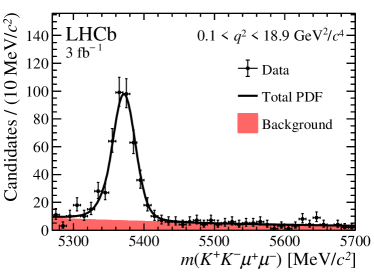
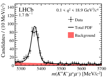
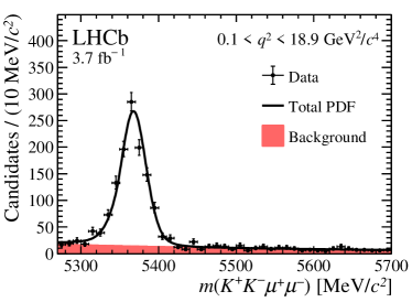
Figure 1: The $m({{K}^{+}}{{K}^{-}}{\mu^{+}\mu^{-}})$ distribution for ${{B}^{0}_{s}}\!\rightarrow\phi{\mu^{+}}{\mu^{-}}$ candidates integrated over the $0.1<{q^{2}}<0.98\text{\,Ge\kern-1.00006ptV}^{2}\!/c^{4}$, $1.1<{q^{2}}<8\text{\,Ge\kern-1.00006ptV}^{2}\!/c^{4}$, $11.0<{q^{2}}<12.5\text{\,Ge\kern-1.00006ptV}^{2}\!/c^{4}$ and $15.0<{q^{2}}<18.9\text{\,Ge\kern-1.00006ptV}^{2}\!/c^{4}$ regions for the data-taking periods 2011-2012 (top left), 2016 (top right), and 2017–2018 (bottom). The data are overlaid with the PDF used to describe the $m({{K}^{+}}{{K}^{-}}{\mu^{+}\mu^{-}})$ spectrum, fitted separately for each data set.

4 Angular analysis

The angular observables are determined using an unbinned maximum likelihood fit to the invariant ${K}^{+}$ ${K}^{-}$ $\mu^{+}\mu^{-}$ mass distribution and the three decay angles, $\theta_{l}$, $\theta_{K}$, and $\phi$. In the $q^{2}$ region below 12.5$\text{\,Ge\kern-1.00006ptV}^{2}\!/c^{4}$, the fit is performed separately in narrow $q^{2}$ regions of around 2$\text{\,Ge\kern-1.00006ptV}^{2}\!/c^{4}$ width and in an additional wide $q^{2}$ region defined as $[1.1,6.0]\text{\,Ge\kern-1.00006ptV}^{2}\!/c^{4}$. Above 15$\text{\,Ge\kern-1.00006ptV}^{2}\!/c^{4}$, a single wide region is used, defined as $[15.0,18.9]\text{\,Ge\kern-1.00006ptV}^{2}\!/c^{4}$. A finer binning scheme compared to Ref. [4] is chosen to maximise sensitivity to potential short-distance NP contributions whilst ensuring stable fit behaviour.

The $m({{K}^{+}}{{K}^{-}}{\mu^{+}\mu^{-}})$ distribution is included in the fit to improve the separation power between signal and background. The signal component is modelled in $m({{K}^{+}}{{K}^{-}}{\mu^{+}\mu^{-}})$ by a sum of two Gaussian functions with a common mean and power-law tails towards the upper or lower mass side [55]. The parameters describing the power-law tails are determined using simulated ${{B}^{0}_{s}}\!\rightarrow{{J\mskip-3.0mu/\mskip-2.0mu\psi}}\phi$ events. The parameters describing the widths and the mean of the Gaussian functions are fixed in the signal mode to the values from a fit to ${{B}^{0}_{s}}\!\rightarrow{{J\mskip-3.0mu/\mskip-2.0mu\psi}}\phi$ candidates in data. An additional $q^{2}$-dependent scaling factor is determined from simulation and applied to the widths of the Gaussian distributions to account for the $q^{2}$ dependence of the $m({{K}^{+}}{{K}^{-}}{\mu^{+}\mu^{-}})$ invariant-mass resolution. The angular distribution for the signal candidates is parameterised using Eq. 1. The combinatorial background in the $m({{K}^{+}}{{K}^{-}}{\mu^{+}\mu^{-}})$ distribution is described using an exponential function and in the angular distributions using a product of first-order Chebyshev polynomials. The factorisation of the background angular distributions is validated using data candidates selected in the upper mass sideband. The fraction of ${{B}^{0}_{s}}\!\rightarrow{{K}^{+}}{{K}^{-}}{\mu^{+}\mu^{-}}$ decays with the ${K}^{+}$ ${K}^{-}$ system in an S-wave configuration, $F_{\rm S}$, is expected to be at the level of 1–2% [56, 57, 58]. These contributions are therefore not modelled in the fit and a systematic uncertainty is assigned to account for this choice.

The selection and reconstruction can distort the angular and $q^{2}$ distributions observed in data. These effects are described by an angular acceptance, $\epsilon(\cos{\theta_{\ell}},\cos{\theta_{K}},\phi,{q^{2}})$. The acceptance is parameterised using a product of Legendre polynomials $P_{i}$ of order $i$ according to

$$\epsilon(\cos{\theta_{\ell}},\cos{\theta_{K}},\phi,{q^{2}})=\sum_{k,l,m,n}c_{klmn}P_{k}(\cos{\theta_{\ell}})P_{l}(\cos{\theta_{K}})P_{m}(\phi)P_{n}({q^{2}})\,,$$ (2)

where the coefficients $c_{klmn}$ are determined on a large sample of simulated ${{B}^{0}_{s}}\!\rightarrow\phi{\mu^{+}}{\mu^{-}}$ events by exploiting the orthogonality of the Legendre polynomials. Given that the acceptance is parameterised in terms of the key degrees of freedom used in the decay description (i.e. the three angles and $q^{2}$) there is minimal dependency on the model used to simulate the events. The orders used to model the efficiency are $k\leq 4$, $l\leq 2$ ($l\leq 4$ in Run 2), $m\leq 6$ and $n\leq 7$ in $\cos{\theta_{\ell}}$, $\cos{\theta_{K}}$, $\phi$ and $q^{2}$, respectively. Where different sets of acceptance orders give a similar description of the acceptance function, the set of lowest orders is chosen. Given the flavour-symmetric final state, only even orders are considered in the description of the three decay angles. The choice of orders used to describe the angular acceptance is assessed as a source of systematic uncertainty.

In the narrow $q^{2}$ regions, the PDF describing the signal candidates is constructed from the product of the acceptance function evaluated at the median of the $q^{2}$ region and the signal fit model. For the wide $q^{2}$ regions, the acceptance is taken into account by weighting each event by the inverse efficiency. The shape of the angular acceptance is found to vary according to the data-taking conditions. The different trigger thresholds during the 2016 and 2017–2018 data-taking periods require the Run 2 data to be further separated. The angular acceptance is therefore derived separately for the 2011–2012, 2016 and 2017–2018 data sets. The data are split according to these periods and a simultaneous fit is performed. In the fit, the angular observables and angular background parameters are shared across the three data sets. The sharing of the angular background parameters improves the fit behaviour and the resulting small bias due to this choice is added as a systematic uncertainty. All other nuisance parameters are determined independently for each data set. In order to avoid experimenter’s bias, all decisions regarding the fit strategy and candidate selection were made before the results were examined.

Pseudoexperiments, generated using the results of the best fit to data, are used to assess the bias and coverage of the simultaneous fit. The majority of observables have a bias of less than 10% of the statistical uncertainty. The observables $S_{3}$ and $S_{4}$ in the $q^{2}$ region $[4.0,6.0]\text{\,Ge\kern-1.00006ptV}^{2}\!/c^{4}$ and $A_{\mathrm{FB}}^{{C\!P}}$ in the $q^{2}$ region $[0.1,0.98]\text{\,Ge\kern-1.00006ptV}^{2}\!/c^{4}$ exhibit a fit bias at the level of 15% of the statistical uncertainty. An additional systematic uncertainty equal to the size of the fit bias is assigned for all observables and the statistical uncertainty is corrected to account for any under- or over-coverage, which is at the level of 14% or less.

The angular acceptance corrections for each data set are validated using both fits to ${{B}^{0}_{s}}\!\rightarrow{{J\mskip-3.0mu/\mskip-2.0mu\psi}}\phi$ candidates and fits to simulated ${{B}^{0}_{s}}\!\rightarrow\phi{\mu^{+}}{\mu^{-}}$ candidates, where the latter are generated according to a physics model using inputs from Ref. [59]. The angular observables extracted from fits to ${{B}^{0}_{s}}\!\rightarrow{{J\mskip-3.0mu/\mskip-2.0mu\psi}}\phi$ candidates are in good agreement with previous measurements [57, 58]. In addition, the angular observables extracted from fits to simulated events are in good agreement with the values used in their generation.

5 Results

The angular distributions for the combined 2011–2012, 2016 and 2017–2018 data set are shown in Fig. 2 for all candidates in the $[1.1,6]\text{\,Ge\kern-1.00006ptV}^{2}\!/c^{4}$ $q^{2}$ region and for candidates within $\pm 50\text{\,Me\kern-1.00006ptV\!/}c^{2}$ of the known ${B}^{0}_{s}$ mass. The data are overlaid with the projection of the fitted PDF, combined across the data sets. The fit projections for all $q^{2}$ regions and individual data sets are provided in Appendix A.

The numerical results for the angular observables are given in Table 1, including systematic uncertainties as discussed in Sec. 6. The linear-correlation matrices for the angular observables are provided in Tables 3, 4 and 5 in Appendix B. A graphical comparison of the results with the SM predictions [23, 24, 25, 26] is shown in Fig. 3. Overall, the results are in good agreement with the SM predictions, with the $C\!P$ asymmetries compatible with zero as expected in the SM. For the $C\!P$ averages, a mild tension in $F_{\mathrm{L}}$ is observed at low $q^{2}$, where the data are found to lie below the SM prediction.

To determine the compatibility of the angular observables with the SM, the flavio software package [24] is used. The Wilson coefficient representing the real part of the $bs\mu\mu$ vector coupling, ${\cal R}e({\cal C}_{9})$, is varied in a fit of the $C\!P$-averaged angular observables $F_{\mathrm{L}}$, $S_{3}$, $S_{4}$ and $S_{7}$ in the $q^{2}$ regions $[0.1,0.98]$, $[1.1,4.0]$, $[4.0,6.0]$ and $[15,18.9]\text{\,Ge\kern-1.00006ptV}^{2}\!/c^{4}$. The $[6.0,8.0]$ and $[11.0,12.5]\text{\,Ge\kern-1.00006ptV}^{2}\!/c^{4}$ regions are excluded from the fit as they are particularly sensitive to long-distance effects from charmonium resonances, which cannot currently be calculated from first principles in the SM [30]. The asymmetries are excluded as they offer little sensitivity to ${\cal R}e({\cal C}_{9})$. The best fit value is given by $\Delta{\cal R}e({\cal C}_{9})=-1.3\,^{+0.7}_{-0.6}$ and is preferred over the SM hypothesis ($\Delta{\cal R}e({\cal C}_{9})=0$) at the level of $1.9\,\sigma$.

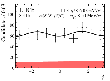
Figure 2: Angular projections in the region $1.1<{q^{2}}<6.0\text{\,Ge\kern-1.00006ptV}^{2}\!/c^{4}$ for the combined 2011–2012, 2016 and 2017–2018 data sets. The data are overlaid with the projection of the combined PDF. The red shaded area indicates the background component and the solid black line the total PDF. The angular projections are given for candidates in (left) the entire mass region used to determine the observables in this paper and (right) the signal mass window $\pm 50\text{\,Me\kern-1.00006ptV\!/}c^{2}$ around the known ${B}^{0}_{s}$ mass.

Table 1: $C\!P$ averages $F_{\mathrm{L}}$ and $S_{3,4,7}$ and $C\!P$ asymmetries $A_{\mathrm{FB}}^{{C\!P}}$ and $A_{5,8,9}$ obtained from the maximum likelihood fit. The first uncertainty is statistical and the second is the total systematic uncertainty, as described in Sec. 6.

$q^{2}$ [$\text{\,Ge\kern-1.00006ptV}^{2}\!/c^{4}$ ]	$F_{\mathrm{L}}$	$S_{3}$	$S_{4}$	$S_{7}$
$[0.1,0.98]$	$0.254\pm 0.045\pm 0.017$	$-0.004\pm 0.068\pm 0.014$	$0.213\pm 0.082\pm 0.005$	$-0.178\pm 0.072\pm 0.001$
$[1.1,4.0]$	$0.723\pm 0.053\pm 0.015$	$-0.030\pm 0.057\pm 0.004$	$-0.110\pm 0.079\pm 0.002$	$-0.101\pm 0.075\pm 0.001$
$[4.0,6.0]$	$0.701\pm 0.050\pm 0.016$	$-0.162\pm 0.067\pm 0.012$	$-0.222\pm 0.092\pm 0.010$	$0.175\pm 0.089\pm 0.003$
$[6.0,8.0]$	$0.624\pm 0.051\pm 0.012$	$0.013\pm 0.080\pm 0.009$	$-0.176\pm 0.078\pm 0.006$	$0.033\pm 0.081\pm 0.002$
$[11.0,12.5]$	$0.353\pm 0.044\pm 0.012$	$-0.138\pm 0.071\pm 0.013$	$-0.319\pm 0.061\pm 0.008$	$-0.170\pm 0.069\pm 0.000$
$[1.1,6.0]$	$0.715\pm 0.036\pm 0.013$	$-0.083\pm 0.047\pm 0.006$	$-0.155\pm 0.058\pm 0.004$	$0.020\pm 0.059\pm 0.001$
$[15.0,18.9]$	$0.359\pm 0.031\pm 0.019$	$-0.247\pm 0.042\pm 0.014$	$-0.208\pm 0.047\pm 0.006$	$0.003\pm 0.046\pm 0.002$

$q^{2}$ [$\text{\,Ge\kern-1.00006ptV}^{2}\!/c^{4}$ ]	$A_{5}$	$A_{\mathrm{FB}}^{{C\!P}}$	$A_{8}$	$A_{9}$
$[0.1,0.98]$	$0.043\pm 0.067\pm 0.001$	$0.068\pm 0.064\pm 0.009$	$-0.007\pm 0.073\pm 0.004$	$-0.030\pm 0.079\pm 0.001$
$[1.1,4.0]$	$0.026\pm 0.067\pm 0.002$	$0.023\pm 0.054\pm 0.001$	$0.038\pm 0.082\pm 0.001$	$0.020\pm 0.068\pm 0.001$
$[4.0,6.0]$	$-0.084\pm 0.084\pm 0.003$	$-0.030\pm 0.051\pm 0.002$	$0.012\pm 0.090\pm 0.002$	$-0.008\pm 0.061\pm 0.001$
$[6.0,8.0]$	$-0.022\pm 0.082\pm 0.001$	$0.032\pm 0.049\pm 0.001$	$-0.170\pm 0.080\pm 0.002$	$-0.012\pm 0.090\pm 0.001$
$[11.0,12.5]$	$0.035\pm 0.063\pm 0.001$	$0.034\pm 0.048\pm 0.001$	$0.046\pm 0.070\pm 0.002$	$0.017\pm 0.071\pm 0.001$
$[1.1,6.0]$	$-0.007\pm 0.051\pm 0.001$	$0.006\pm 0.036\pm 0.001$	$0.016\pm 0.062\pm 0.001$	$0.009\pm 0.046\pm 0.001$
$[15.0,18.9]$	$-0.025\pm 0.043\pm 0.001$	$-0.011\pm 0.033\pm 0.001$	$0.072\pm 0.051\pm 0.002$	$0.021\pm 0.042\pm 0.001$

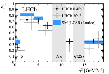
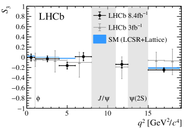
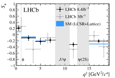
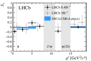
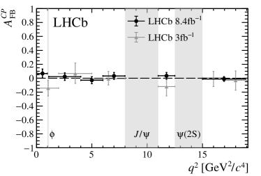
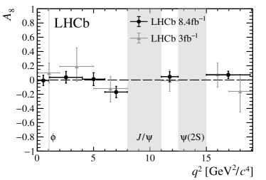
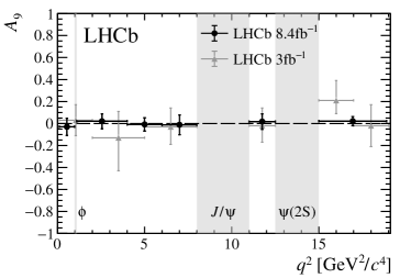
Figure 3: $C\!P$-averaged angular observables $F_{\mathrm{L}}$ and $S_{3,4,7}$ and $C\!P$-asymmetries $A_{\mathrm{FB}}^{{C\!P}}$ and $A_{5,8,9}$ shown by black crosses, overlaid with the SM prediction [23, 24, 25, 26] as blue boxes, where available. The grey crosses indicate the results from Ref. [4]. The grey bands indicate the regions of the charmonium resonances and the ${{B}^{0}_{s}}\!\rightarrow\phi\phi$ region.

6 Systematic uncertainties

Systematic effects may change the measured angular observables. The size of these effects is determined using high-yield pseudoexperiments, generated using an alternative PDF which encodes the systematic effect under study. The pseudoexperiments are fitted with both the default and alternative PDFs, and the resulting difference in angular observables is assigned as a systematic uncertainty. Each systematic effect is studied using approximately one hundred million generated events.

The simulated samples used to derive the default acceptance are produced according to the phase space of the three-body ${{B}^{0}_{s}}\!\rightarrow\phi{\mu^{+}}{\mu^{-}}$ decay with the lifetime difference between the ${B}^{0}_{s}$ and ${\kern 1.79993pt\overline{\kern-1.79993ptB}}{}^{0}_{s}$ system, $\Delta\Gamma_{s}$, set to zero. A systematic uncertainty is determined by weighting the angular, $q^{2}$ and ${B}^{0}_{s}$ lifetime distributions of simulated events to an alternative model description, in which the value for $\Delta\Gamma_{s}/\Gamma_{s}$ is taken as 0.17 [60] and the ${{B}^{0}_{s}}\!\rightarrow\phi{\mu^{+}}{\mu^{-}}$ decay is described using a more realistic physics model with form factor calculations taken from Refs. [23, 24, 25, 26].

As the angular observables are measured integrated over the ${B}^{0}_{s}$ decay time, neglecting the ${{B}^{0}_{s}}$ decay time dependence of the acceptance induces an additional source of bias. The size of this effect remains small compared to the statistical uncertainty and is accounted for with a systematic uncertainty.

To assess the systematic uncertainty associated with the description of the angular background distribution, pseudoexperiments are generated using second-order Chebyshev polynomials, the coefficients for which are obtained from a fit to candidates in the upper mass sideband. Similarly, the impact of sharing the angular background parameters across data sets is determined by generating pseudoexperiments using first order Chebyshev polynomials with coefficients derived separately for each data set.

To evaluate the impact of the corrections to the track multiplicity, ${B}^{0}_{s}$ $p_{\mathrm{T}}$ spectrum and hardware trigger response in simulated events on the angular observables, the angular acceptance is rederived, each time removing a correction. The largest resulting deviation in a given angular observable is assigned as a systematic uncertainty. For the particle identification response, the corrections are determined using an alternative model and a new angular acceptance is rederived.

To account for neglected ${{B}^{0}_{s}}\!\rightarrow{{K}^{+}}{{K}^{-}}{\mu^{+}\mu^{-}}$ decays, where the ${{K}^{+}}{{K}^{-}}$ system is in an S-wave configuration, pseudoexperiments are generated according to the combined P- and S-wave decay rate, where $F_{\rm S}$ is conservatively taken to be 2%. The pseudoexperiments are fitted with the default model and the resulting shift in the angular observables is assigned as a systematic uncertainty. The impact of peaking background contributions is assessed in a similar fashion by injecting additional events drawn from the reconstructed ${B}^{0}_{s}$ mass and angular distributions of the background in question.

The influence of the choice for the maximum order of the Legendre polynomials used in the acceptance parameterisation is evaluated by rederiving the acceptance using a higher order. Further sources of systematic uncertainty include the size of the simulated samples used to derive the acceptance, the evaluation of the acceptance at a single point in $q^{2}$ for the narrow $q^{2}$ regions and the signal mass model, all of which yield negligible contributions to the overall systematic uncertainty.

The systematic uncertainties are summarised in Table 2. As the size of a systematic effect can vary strongly depending on the observable and $q^{2}$ region in question, only the magnitude of the largest systematic uncertainty across all regions, rounded up to the next multiple of 0.005, is indicated.

Table 2: Sources of the systematic uncertainties associated with the angular observables. As the size of a systematic effect can vary strongly depending on the observable and $q^{2}$ region in question, only the magnitude of the largest systematic uncertainty across all regions, rounded up to the next multiple of 0.005, is indicated.

Systematic source	$F_{\mathrm{L}}$	$S_{3,4,7}$	$A_{5,8,9},A_{\mathrm{FB}}^{{C\!P}}$
Physics model	$<0.015$	$<0.015$	$<0.005$
Time integration	$<0.010$	$<0.010$	$<0.005$
Fit bias	$<0.005$	$<0.015$	$<0.010$
Angular background model	$<0.015$	$<0.005$	$<0.005$
Simulation corrections	$<0.015$	$<0.005$	$<0.005$
S-wave and peaking bkg.	$<0.010$	$<0.010$	$<0.005$
Acceptance order	$<0.010$	$<0.005$	$<0.005$
Simulation statistics	$<0.010$	$<0.005$	$<0.005$
Signal mass model	$<0.005$	$<0.005$	$<0.005$
$q^{2}$ evaluation point	$<0.005$	$<0.005$	$<0.005$

7 Conclusions

This paper presents an angular analysis of the ${{B}^{0}_{s}}\!\rightarrow\phi{\mu^{+}}{\mu^{-}}$ decay using $pp$ collisions corresponding to 8.4 $\text{\,fb}^{-1}$ of data recorded by the LHCb experiment during the Run 1 and Run 2 data-taking periods. The angular observables are extracted using an unbinned maximum likelihood fit to the angular distributions of untagged ${{B}^{0}_{s}}\!\rightarrow\phi{\mu^{+}}{\mu^{-}}$ decays in regions of the square of the dimuon mass, $q^{2}$. The results in this paper constitute the most precise measurement of the ${{B}^{0}_{s}}\!\rightarrow\phi{\mu^{+}}{\mu^{-}}$ angular observables to date, with an approximate two-fold increase in sensitivity compared to the results of Ref. [4], which are superseded by this paper. The results are found to be compatible with SM predictions.

Appendices

Appendix A Fit projections for the rare decay ${{B}^{0}_{s}}\!\rightarrow\phi{\mu^{+}}{\mu^{-}}$

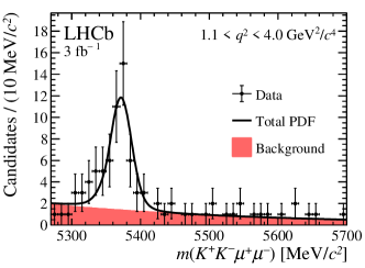
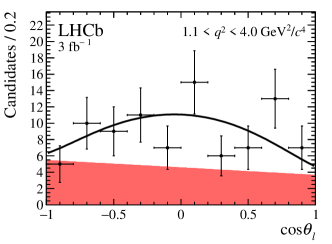
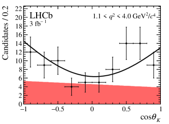
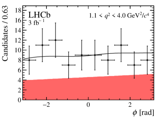
Figure 15: Mass and angular distributions of ${{B}^{0}_{s}}\!\rightarrow\phi{\mu^{+}}{\mu^{-}}$ candidates in the region $1.1<{q^{2}}<4.0\text{\,Ge\kern-1.00006ptV}^{2}\!/c^{4}$ for data taken in 2011–2012. The data are overlaid with the projections of the fitted PDF.

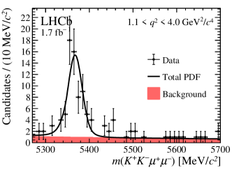
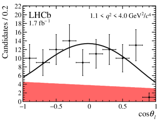
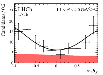
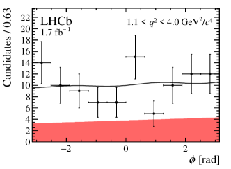
Figure 16: Mass and angular distributions of ${{B}^{0}_{s}}\!\rightarrow\phi{\mu^{+}}{\mu^{-}}$ candidates in the region $1.1<{q^{2}}<4.0\text{\,Ge\kern-1.00006ptV}^{2}\!/c^{4}$ for data taken in 2016. The data are overlaid with the projections of the fitted PDF.

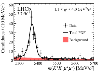
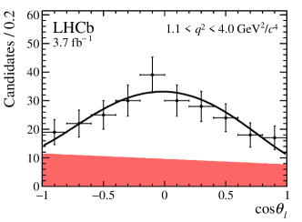
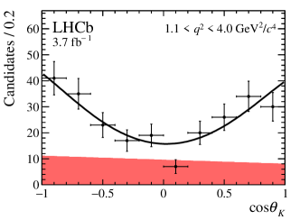
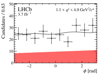
Figure 17: Mass and angular distributions of ${{B}^{0}_{s}}\!\rightarrow\phi{\mu^{+}}{\mu^{-}}$ candidates in the region $1.1<{q^{2}}<4.0\text{\,Ge\kern-1.00006ptV}^{2}\!/c^{4}$ for data taken in 2017–2018. The data are overlaid with the projections of the fitted PDF.

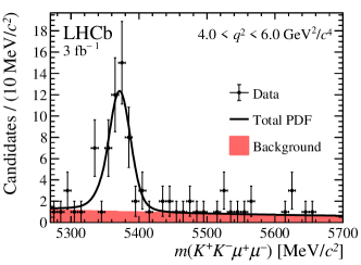
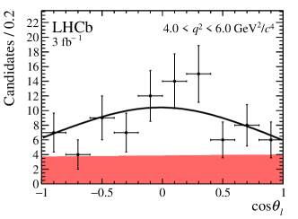
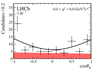
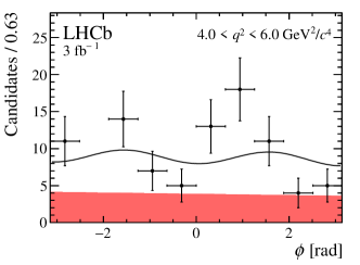
Figure 18: Mass and angular distributions of ${{B}^{0}_{s}}\!\rightarrow\phi{\mu^{+}}{\mu^{-}}$ candidates in the region $4.0<{q^{2}}<6.0\text{\,Ge\kern-1.00006ptV}^{2}\!/c^{4}$ for data taken in 2011–2012. The data are overlaid with the projections of the fitted PDF.

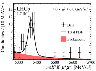
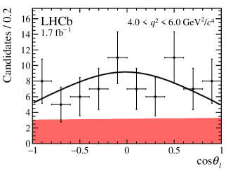
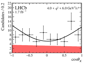
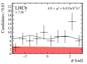
Figure 19: Mass and angular distributions of ${{B}^{0}_{s}}\!\rightarrow\phi{\mu^{+}}{\mu^{-}}$ candidates in the region $4.0<{q^{2}}<6.0\text{\,Ge\kern-1.00006ptV}^{2}\!/c^{4}$ for data taken in 2016. The data are overlaid with the projections of the fitted PDF.

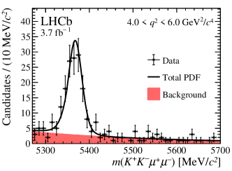
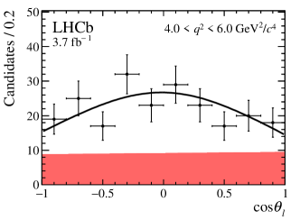
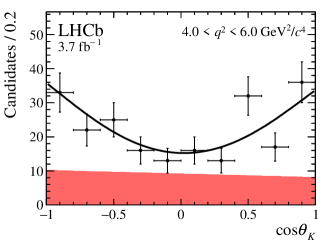
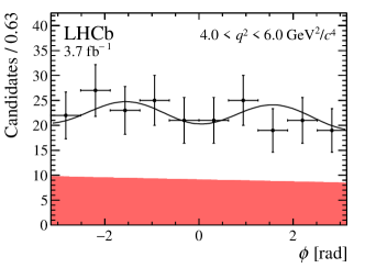
Figure 20: Mass and angular distributions of ${{B}^{0}_{s}}\!\rightarrow\phi{\mu^{+}}{\mu^{-}}$ candidates in the region $4.0<{q^{2}}<6.0\text{\,Ge\kern-1.00006ptV}^{2}\!/c^{4}$ for data taken in 2017–2018. The data are overlaid with the projections of the fitted PDF.

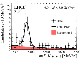
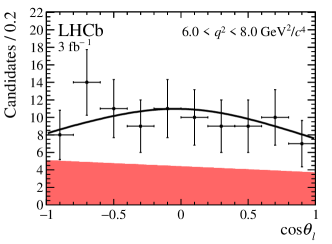
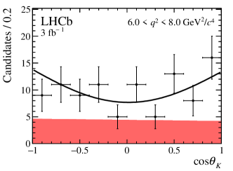
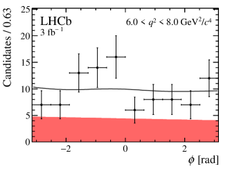
Figure 21: Mass and angular distributions of ${{B}^{0}_{s}}\!\rightarrow\phi{\mu^{+}}{\mu^{-}}$ candidates in the region $6.0<{q^{2}}<8.0\text{\,Ge\kern-1.00006ptV}^{2}\!/c^{4}$ for data taken in 2011–2012. The data are overlaid with the projections of the fitted PDF.

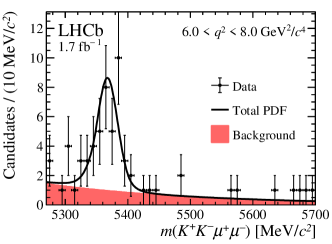
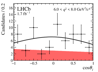
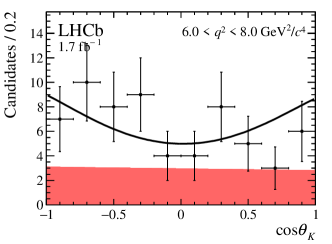
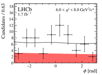
Figure 22: Mass and angular distributions of ${{B}^{0}_{s}}\!\rightarrow\phi{\mu^{+}}{\mu^{-}}$ candidates in the region $6.0<{q^{2}}<8.0\text{\,Ge\kern-1.00006ptV}^{2}\!/c^{4}$ for data taken in 2016. The data are overlaid with the projections of the fitted PDF.

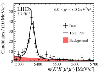
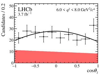
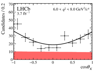
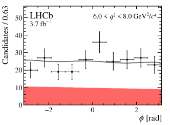
Figure 23: Mass and angular distributions of ${{B}^{0}_{s}}\!\rightarrow\phi{\mu^{+}}{\mu^{-}}$ candidates in the region $6.0<{q^{2}}<8.0\text{\,Ge\kern-1.00006ptV}^{2}\!/c^{4}$ for data taken in 2017–2018. The data are overlaid with the projections of the fitted PDF.

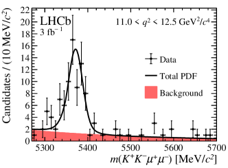
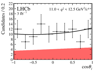
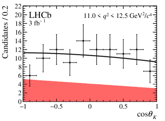
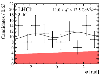
Figure 24: Mass and angular distributions of ${{B}^{0}_{s}}\!\rightarrow\phi{\mu^{+}}{\mu^{-}}$ candidates in the region $11.0<{q^{2}}<12.5\text{\,Ge\kern-1.00006ptV}^{2}\!/c^{4}$ for data taken in 2011–2012. The data are overlaid with the projections of the fitted PDF.

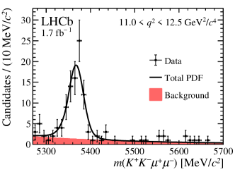
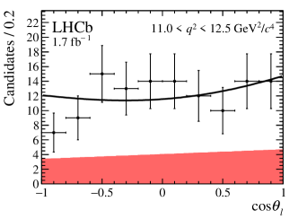
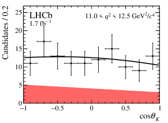
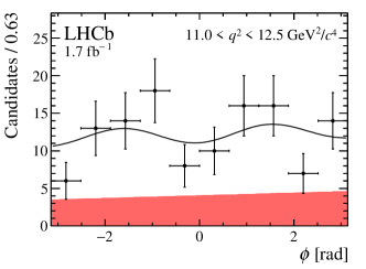
Figure 25: Mass and angular distributions of ${{B}^{0}_{s}}\!\rightarrow\phi{\mu^{+}}{\mu^{-}}$ candidates in the region $11.0<{q^{2}}<12.5\text{\,Ge\kern-1.00006ptV}^{2}\!/c^{4}$ for data taken in 2016. The data are overlaid with the projections of the fitted PDF.

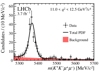
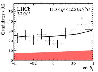
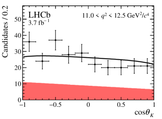
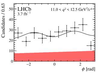
Figure 26: Mass and angular distributions of ${{B}^{0}_{s}}\!\rightarrow\phi{\mu^{+}}{\mu^{-}}$ candidates in the region $11.0<{q^{2}}<12.5\text{\,Ge\kern-1.00006ptV}^{2}\!/c^{4}$ for data taken in 2017–2018. The data are overlaid with the projections of the fitted PDF.

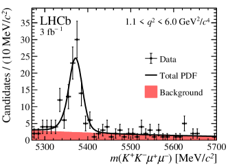
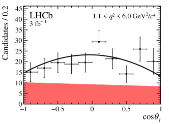
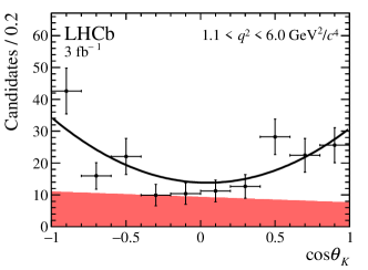
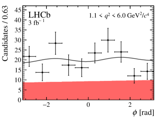
Figure 27: Mass and angular distributions of ${{B}^{0}_{s}}\!\rightarrow\phi{\mu^{+}}{\mu^{-}}$ candidates in the region $1.1<{q^{2}}<6.0\text{\,Ge\kern-1.00006ptV}^{2}\!/c^{4}$ for data taken in 2011–2012. The data are overlaid with the projections of the fitted PDF.

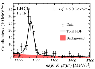
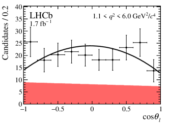
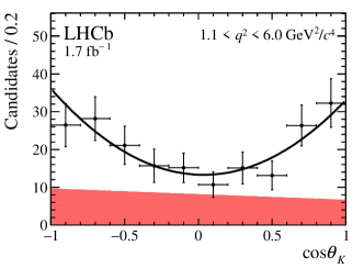
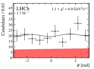
Figure 28: Mass and angular distributions of ${{B}^{0}_{s}}\!\rightarrow\phi{\mu^{+}}{\mu^{-}}$ candidates in the region $1.1<{q^{2}}<6.0\text{\,Ge\kern-1.00006ptV}^{2}\!/c^{4}$ for data taken in 2016. The data are overlaid with the projections of the fitted PDF.

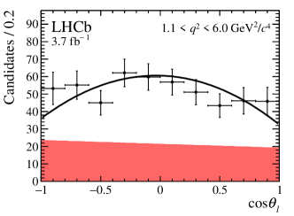
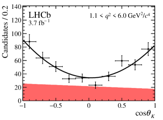
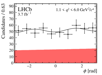
Figure 29: Mass and angular distributions of ${{B}^{0}_{s}}\!\rightarrow\phi{\mu^{+}}{\mu^{-}}$ candidates in the region $1.1<{q^{2}}<6.0\text{\,Ge\kern-1.00006ptV}^{2}\!/c^{4}$ for data taken in 2017–2018. The data are overlaid with the projections of the fitted PDF.

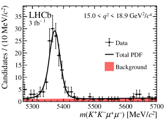
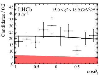
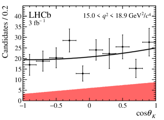
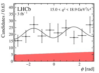
Figure 30: Mass and angular distributions of ${{B}^{0}_{s}}\!\rightarrow\phi{\mu^{+}}{\mu^{-}}$ candidates in the region $15.0<{q^{2}}<18.9\text{\,Ge\kern-1.00006ptV}^{2}\!/c^{4}$ for data taken in 2011–2012. The data are overlaid with the projections of the fitted PDF.

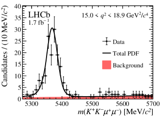
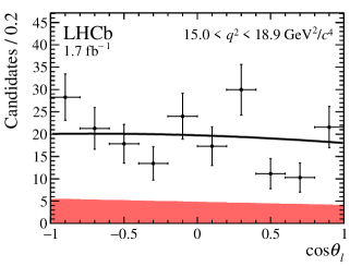
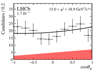
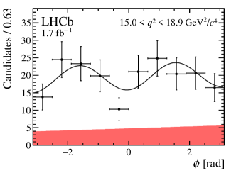
Figure 31: Mass and angular distributions of ${{B}^{0}_{s}}\!\rightarrow\phi{\mu^{+}}{\mu^{-}}$ candidates in the region $15.0<{q^{2}}<18.9\text{\,Ge\kern-1.00006ptV}^{2}\!/c^{4}$ for data taken in 2016. The data are overlaid with the projections of the fitted PDF.

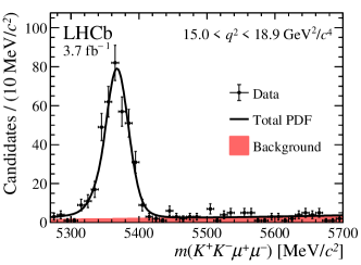
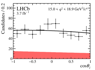
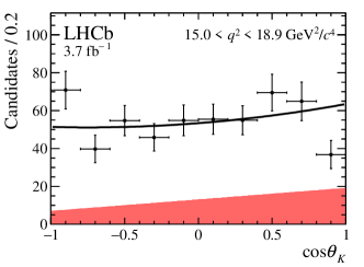
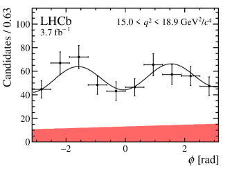
Figure 32: Mass and angular distributions of ${{B}^{0}_{s}}\!\rightarrow\phi{\mu^{+}}{\mu^{-}}$ candidates in the region $15.0<{q^{2}}<18.9\text{\,Ge\kern-1.00006ptV}^{2}\!/c^{4}$ for data taken in 2017–2018. The data are overlaid with the projections of the fitted PDF.

The mass distributions for the combined 2011–2012, 2016 and 2017–2018 data sets for each $q^{2}$ region are shown in Fig. 4. The corresponding angular distributions are shown in Figs. 5–11, for all candidates and the candidates within the signal mass region $\pm 50\text{\,Me\kern-1.00006ptV\!/}c^{2}$ around the known ${B}^{0}_{s}$ mass. The data are overlaid with the projections of the fitted PDF, combined across the data sets. The projections of the mass and angular distributions, for each data set and $q^{2}$ region separately, are shown in Figs. 12–32. All three data sets used in this analysis are fitted simultaneously.

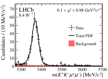
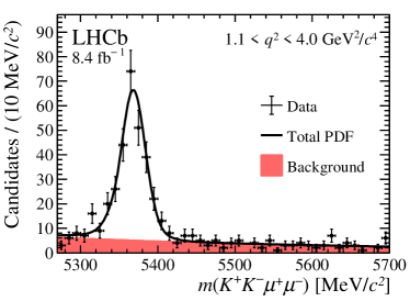
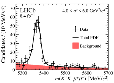
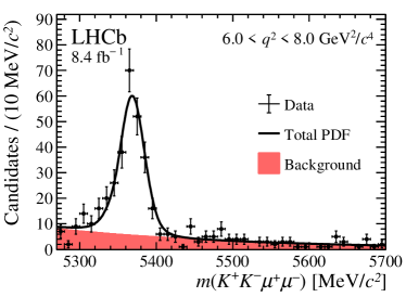
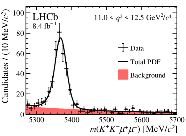
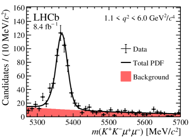
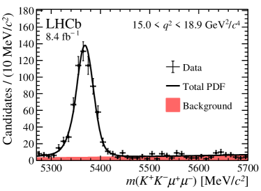
Figure 4: Mass distributions of ${{B}^{0}_{s}}\!\rightarrow\phi{\mu^{+}}{\mu^{-}}$ candidates in the different $q^{2}$ regions for the combined 2011–2012, 2016 and 2017–2018 data sets. The data are overlaid with the projection of the combined PDF. The red shaded area indicates the background component and the solid black line the total PDF.

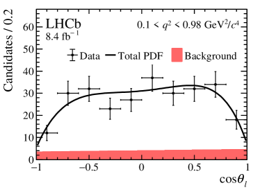
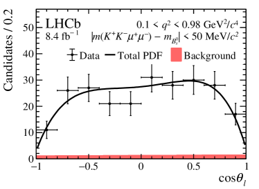
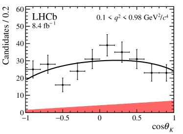
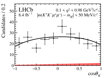
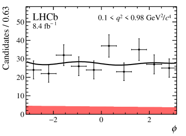
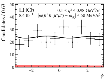
Figure 5: Projections in the region $0.1<{q^{2}}<0.98\text{\,Ge\kern-1.00006ptV}^{2}\!/c^{4}$ for the angular distributions of the combined 2011–2012, 2016 and 2017–2018 data sets. The data are overlaid with the projection of the combined PDF. The red shaded area indicates the background component and the solid black line the total PDF. The angular projections are given for candidates in (left) the entire mass region used to determine the observables in this paper and (right) the signal mass window $\pm 50\text{\,Me\kern-1.00006ptV\!/}c^{2}$ around the known ${B}^{0}_{s}$ mass.

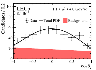
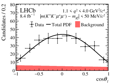
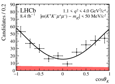
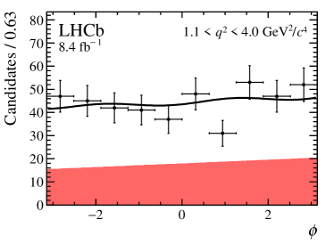
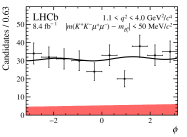
Figure 6: Projections in the region $1.1<{q^{2}}<4.0\text{\,Ge\kern-1.00006ptV}^{2}\!/c^{4}$ for the angular distributions of the combined 2011–2012, 2016 and 2017–2018 data set. The data are overlaid with the projection of the combined PDF. The red shaded area indicates the background component and the solid black line the total PDF. The angular projections are given for candidates in (left) the entire mass region used to determine the observables in this paper and (right) the signal mass window $\pm 50\text{\,Me\kern-1.00006ptV\!/}c^{2}$ around the known ${B}^{0}_{s}$ mass.

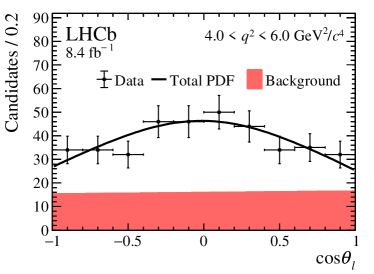
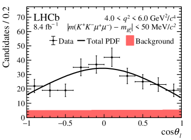
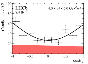
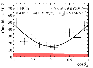
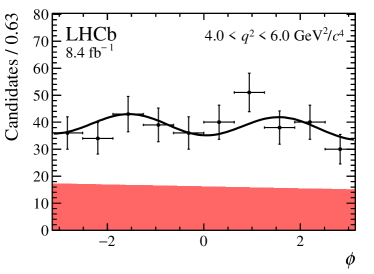
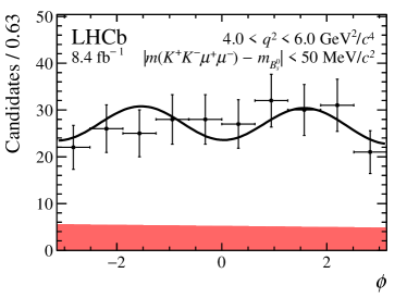
Figure 7: Projections in the region $4.0<{q^{2}}<6.0\text{\,Ge\kern-1.00006ptV}^{2}\!/c^{4}$ for the angular distributions of the combined 2011–2012, 2016 and 2017–2018 data sets. The data are overlaid with the projection of the combined PDF. The red shaded area indicates the background component and the solid black line the total PDF. The angular projections are given for candidates in (left) the entire mass region used to determine the observables in this paper and (right) the signal mass window $\pm 50\text{\,Me\kern-1.00006ptV\!/}c^{2}$ around the known ${B}^{0}_{s}$ mass.

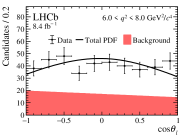
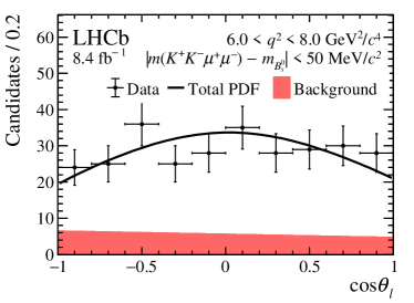
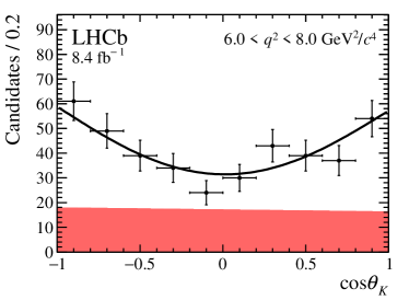
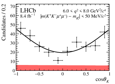
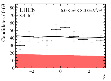
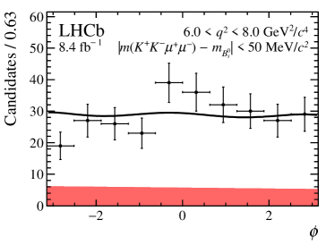
Figure 8: Projections in the region $6.0<{q^{2}}<8.0\text{\,Ge\kern-1.00006ptV}^{2}\!/c^{4}$ for the angular distributions of the combined 2011–2012, 2016 and 2017–2018 data sets. The data are overlaid with the projection of the combined PDF. The red shaded area indicates the background component and the solid black line the total PDF. The angular projections are given for candidates in (left) the entire mass region used to determine the observables in this paper and (right) the signal mass window $\pm 50\text{\,Me\kern-1.00006ptV\!/}c^{2}$ around the known ${B}^{0}_{s}$ mass.

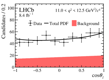
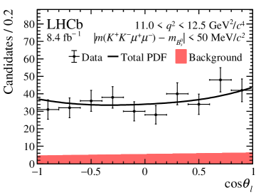
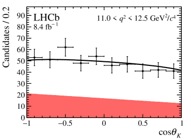
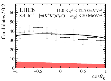
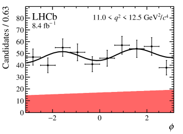
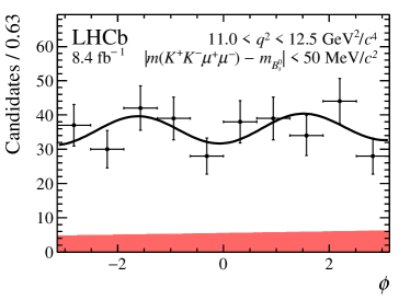
Figure 9: Projections in the region $11.0<{q^{2}}<12.5\text{\,Ge\kern-1.00006ptV}^{2}\!/c^{4}$ for the angular distributions of the combined 2011–2012, 2016 and 2017–2018 data sets. The data are overlaid with the projection of the combined PDF. The red shaded area indicates the background component and the solid black line the total PDF. The angular projections are given for candidates in (left) the entire mass region used to determine the observables in this paper and (right) the signal mass window $\pm 50\text{\,Me\kern-1.00006ptV\!/}c^{2}$ around the known ${B}^{0}_{s}$ mass.

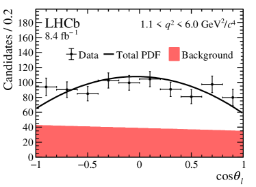
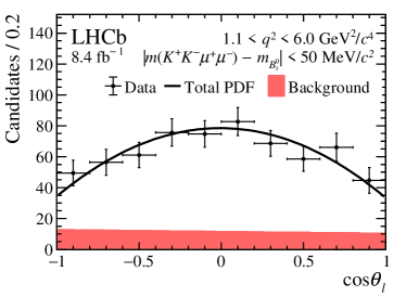
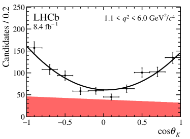
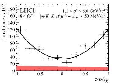
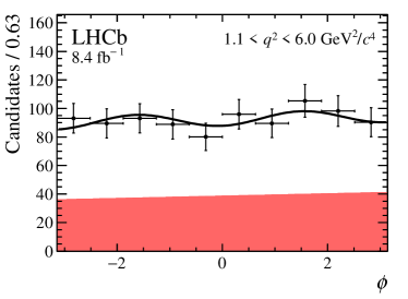
Figure 10: Projections in the region $1.1<{q^{2}}<6.0\text{\,Ge\kern-1.00006ptV}^{2}\!/c^{4}$ for the angular distributions of the combined 2011–2012, 2016 and 2017–2018 data sets. The data are overlaid with the projection of the combined PDF. The red shaded area indicates the background component and the solid black line the total PDF. The angular projections are given for candidates in (left) the entire mass region used to determine the observables in this paper and (right) the signal mass window $\pm 50\text{\,Me\kern-1.00006ptV\!/}c^{2}$ around the known ${B}^{0}_{s}$ mass.

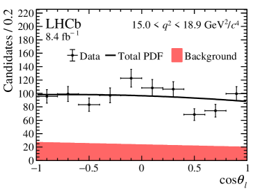
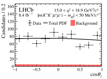
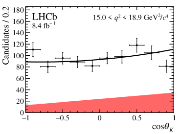
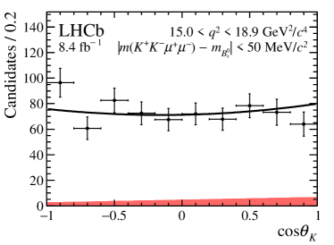
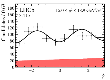
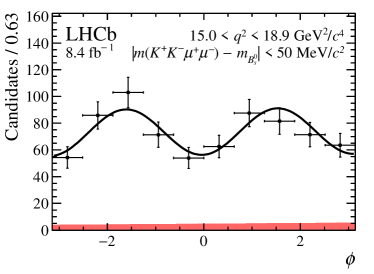
Figure 11: Projections in the region $15.0<{q^{2}}<18.9\text{\,Ge\kern-1.00006ptV}^{2}\!/c^{4}$ for the angular distributions of the combined 2011–2012, 2016 and 2017–2018 data sets. The data are overlaid with the projection of the combined PDF. The red shaded area indicates the background component and the solid black line the total PDF. The angular projections are given for candidates in (left) the entire mass region used to determine the observables in this paper and (right) the signal mass window $\pm 50\text{\,Me\kern-1.00006ptV\!/}c^{2}$ around the known ${B}^{0}_{s}$ mass.

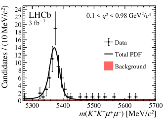
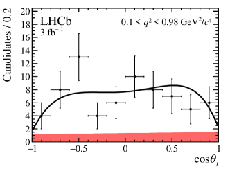
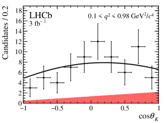
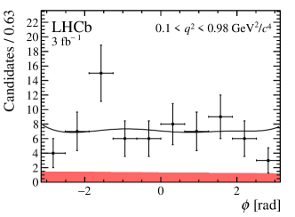
Figure 12: Mass and angular distributions of ${{B}^{0}_{s}}\!\rightarrow\phi{\mu^{+}}{\mu^{-}}$ candidates in the region $0.1<{q^{2}}<0.98\text{\,Ge\kern-1.00006ptV}^{2}\!/c^{4}$ for data taken in 2011–2012. The data are overlaid with the projections of the fitted PDF.

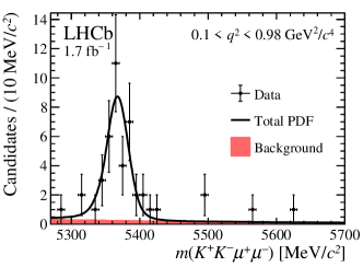
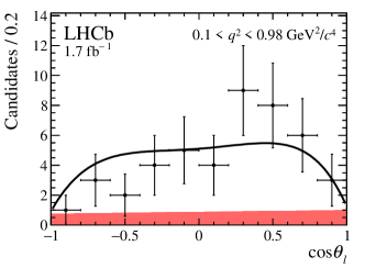
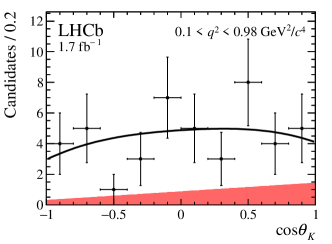
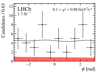
Figure 13: Mass and angular distributions of ${{B}^{0}_{s}}\!\rightarrow\phi{\mu^{+}}{\mu^{-}}$ candidates in the region $0.1<{q^{2}}<0.98\text{\,Ge\kern-1.00006ptV}^{2}\!/c^{4}$ for data taken in 2016. The data are overlaid with the projections of the fitted PDF.

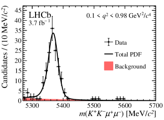
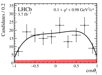
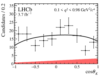
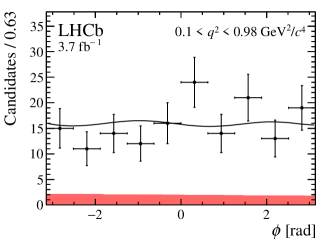
Figure 14: Mass and angular distributions of ${{B}^{0}_{s}}\!\rightarrow\phi{\mu^{+}}{\mu^{-}}$ candidates in the region $0.1<{q^{2}}<0.98\text{\,Ge\kern-1.00006ptV}^{2}\!/c^{4}$ for data taken in 2017–2018. The data are overlaid with the projections of the fitted PDF.

Appendix B Correlation matrices

The linear correlations obtained from the fit of the angular observables are given in Tables 3–5.

Table 3: Correlation matrix for the $q^{2}$ regions $0.1<{q^{2}}<0.98\text{\,Ge\kern-1.00006ptV}^{2}\!/c^{4}$ and $1.1<{q^{2}}<4.0\text{\,Ge\kern-1.00006ptV}^{2}\!/c^{4}$.

Correlation matrix for $0.1<q^{2}<0.98\text{\,Ge\kern-1.00006ptV}^{2}\!/c^{4}$
	$F_{\rm L}$	$S_{3}$	$S_{4}$	$A_{5}$	$A_{\rm FB}^{C\!P}$	$S_{7}$	$A_{8}$	$A_{9}$
$F_{\rm L}$	$1.0$0	$-0.03$	$0.06$	$0.10$	$0.02$	$-0.20$	$-0.05$	$-0.04$
$S_{3}$		$1.00$	$0.11$	$0.00$	$-0.06$	$0.07$	$-0.05$	$0.02$
$S_{4}$			$1.00$	$0.03$	$-0.06$	$0.08$	$-0.05$	$-0.01$
$A_{5}$				$1.00$	$0.12$	$-0.07$	$0.06$	$-0.09$
$A_{\rm FB}^{C\!P}$					$1.00$	$0.02$	$-0.04$	$0.07$
$S_{7}$						$1.00$	$0.29$	$-0.03$
$A_{8}$							$1.00$	$0.06$
$A_{9}$								$1.00$

Correlation matrix for $1.1<q^{2}<4.0\text{\,Ge\kern-1.00006ptV}^{2}\!/c^{4}$
	$F_{\rm L}$	$S_{3}$	$S_{4}$	$A_{5}$	$A_{\rm FB}^{C\!P}$	$S_{7}$	$A_{8}$	$A_{9}$
$F_{\rm L}$	$1.00$	$-0.12$	$0.03$	$-0.03$	$-0.07$	$-0.12$	$0.03$	$-0.01$
$S_{3}$		$1.00$	$-0.07$	$-0.00$	$0.03$	$0.04$	$-0.04$	$0.05$
$S_{4}$			$1.00$	$0.02$	$0.09$	$0.01$	$-0.02$	$-0.02$
$A_{5}$				$1.00$	$-0.08$	$0.02$	$0.01$	$0.06$
$A_{\rm FB}^{C\!P}$					$1.00$	$0.02$	$-0.02$	$0.03$
$S_{7}$						$1.00$	$-0.06$	$0.06$
$A_{8}$							$1.00$	$-0.04$
$A_{9}$								$1.00$

Table 4: Correlation matrix for the $q^{2}$ regions $4.0<{q^{2}}<6.0\text{\,Ge\kern-1.00006ptV}^{2}\!/c^{4}$, $6.0<{q^{2}}<8.0\text{\,Ge\kern-1.00006ptV}^{2}\!/c^{4}$ and $11.0<{q^{2}}<12.5\text{\,Ge\kern-1.00006ptV}^{2}\!/c^{4}$.

Correlation matrix for $4.0<q^{2}<6.0\text{\,Ge\kern-1.00006ptV}^{2}\!/c^{4}$
	$F_{\rm L}$	$S_{3}$	$S_{4}$	$A_{5}$	$A_{\rm FB}^{C\!P}$	$S_{7}$	$A_{8}$	$A_{9}$
$F_{\rm L}$	$1.00$	$0.15$	$0.06$	$-0.08$	$0.01$	$-0.01$	$-0.04$	$-0.08$
$S_{3}$		$1.00$	$-0.04$	$-0.02$	$0.05$	$-0.06$	$-0.04$	$0.22$
$S_{4}$			$1.00$	$-0.12$	$-0.02$	$0.05$	$-0.04$	$-0.07$
$A_{5}$				$1.00$	$-0.11$	$-0.06$	$0.04$	$0.05$
$A_{\rm FB}^{C\!P}$					$1.00$	$-0.01$	$0.10$	$0.01$
$S_{7}$						$1.00$	$-0.13$	$0.02$
$A_{8}$							$1.00$	$-0.05$
$A_{9}$								$1.00$

Correlation matrix for $6.0<q^{2}<8.0\text{\,Ge\kern-1.00006ptV}^{2}\!/c^{4}$
	$F_{\rm L}$	$S_{3}$	$S_{4}$	$A_{5}$	$A_{\rm FB}^{C\!P}$	$S_{7}$	$A_{8}$	$A_{9}$
$F_{\rm L}$	$1.00$	$0.03$	$0.07$	$-0.04$	$-0.10$	$0.01$	$-0.03$	$-0.04$
$S_{3}$		$1.00$	$-0.08$	$-0.02$	$-0.02$	$-0.01$	$0.04$	$-0.05$
$S_{4}$			$1.00$	$-0.09$	$0.02$	$-0.05$	$-0.08$	$-0.06$
$A_{5}$				$1.00$	$-0.12$	$-0.05$	$-0.05$	$0.05$
$A_{\rm FB}^{C\!P}$					$1.00$	$-0.04$	$-0.04$	$-0.01$
$S_{7}$						$1.00$	$-0.14$	$0.03$
$A_{8}$							$1.00$	$-0.05$
$A_{9}$								$1.00$

Correlation matrix for $11.0<q^{2}<12.5\text{\,Ge\kern-1.00006ptV}^{2}\!/c^{4}$
	$F_{\rm L}$	$S_{3}$	$S_{4}$	$A_{5}$	$A_{\rm FB}^{C\!P}$	$S_{7}$	$A_{8}$	$A_{9}$
$F_{\rm L}$	$1.00$	$0.09$	$0.02$	$-0.05$	$-0.10$	$-0.03$	$-0.04$	$-0.07$
$S_{3}$		$1.00$	$-0.14$	$-0.01$	$-0.02$	$0.11$	$-0.06$	$-0.06$
$S_{4}$			$1.00$	$-0.04$	$0.18$	$-0.01$	$-0.07$	$-0.05$
$A_{5}$				$1.00$	$-0.23$	$-0.11$	$0.01$	$-0.02$
$A_{\rm FB}^{C\!P}$					$1.00$	$0.04$	$-0.06$	$0.02$
$S_{7}$						$1.00$	$0.06$	$-0.05$
$A_{8}$							$1.00$	$-0.11$
$A_{9}$								$1.00$

Table 5: Correlation matrix for the $q^{2}$ region $1.1<{q^{2}}<6.0\text{\,Ge\kern-1.00006ptV}^{2}\!/c^{4}$ and $15.0<{q^{2}}<18.9\text{\,Ge\kern-1.00006ptV}^{2}\!/c^{4}$.

Correlation matrix for $1.1<q^{2}<6.0\text{\,Ge\kern-1.00006ptV}^{2}\!/c^{4}$
	$F_{\rm L}$	$S_{3}$	$S_{4}$	$A_{5}$	$A_{\rm FB}^{C\!P}$	$S_{7}$	$A_{8}$	$A_{9}$
$F_{\rm L}$	$1.00$	$-0.03$	$0.05$	$-0.02$	$-0.07$	$-0.08$	$-0.04$	$-0.03$
$S_{3}$		$1.00$	$-0.07$	$0.01$	$0.03$	$-0.07$	$-0.07$	$0.10$
$S_{4}$			$1.00$	$-0.00$	$-0.00$	$-0.06$	$-0.02$	$-0.01$
$A_{5}$				$1.00$	$-0.07$	$-0.00$	$0.05$	$0.08$
$A_{\rm FB}^{C\!P}$					$1.00$	$0.01$	$0.05$	$0.07$
$S_{7}$						$1.00$	$-0.08$	$0.01$
$A_{8}$							$1.00$	$-0.03$
$A_{9}$								$1.00$

Correlation matrix for $15.0<q^{2}<18.9\text{\,Ge\kern-1.00006ptV}^{2}\!/c^{4}$
	$F_{\rm L}$	$S_{3}$	$S_{4}$	$A_{5}$	$A_{\rm FB}^{C\!P}$	$S_{7}$	$A_{8}$	$A_{9}$
$F_{\rm L}$	$1.00$	$0.20$	$-0.04$	$-0.03$	$0.03$	$0.00$	$-0.03$	$-0.10$
$S_{3}$		$1.00$	$-0.06$	$0.03$	$-0.11$	$-0.08$	$0.00$	$0.13$
$S_{4}$			$1.00$	$-0.13$	$-0.03$	$-0.04$	$0.13$	$0.06$
$A_{5}$				$1.00$	$-0.11$	$0.05$	$-0.08$	$0.05$
$A_{\rm FB}^{C\!P}$					$1.00$	$0.10$	$-0.00$	$-0.03$
$S_{7}$						$1.00$	$0.03$	$0.01$
$A_{8}$							$1.00$	$-0.07$
$A_{9}$								$1.00$

LHCb collaboration

R. Aaij³², A.S.W. Abdelmotteleb⁵⁶, C. Abellán Beteta⁵⁰, T. Ackernley⁶⁰, B. Adeva⁴⁶, M. Adinolfi⁵⁴, H. Afsharnia⁹, C. Agapopoulou¹³, C.A. Aidala⁸⁶, S. Aiola²⁵, Z. Ajaltouni⁹, S. Akar⁶⁵, J. Albrecht¹⁵, F. Alessio⁴⁸, M. Alexander⁵⁹, A. Alfonso Albero⁴⁵, Z. Aliouche⁶², G. Alkhazov³⁸, P. Alvarez Cartelle⁵⁵, S. Amato², J.L. Amey⁵⁴, Y. Amhis¹¹, L. An⁴⁸, L. Anderlini²², A. Andreianov³⁸, M. Andreotti²¹, F. Archilli¹⁷, A. Artamonov⁴⁴, M. Artuso⁶⁸, K. Arzymatov⁴², E. Aslanides¹⁰, M. Atzeni⁵⁰, B. Audurier¹², S. Bachmann¹⁷, M. Bachmayer⁴⁹, J.J. Back⁵⁶, P. Baladron Rodriguez⁴⁶, V. Balagura¹², W. Baldini²¹, J. Baptista Leite¹, M. Barbetti²², R.J. Barlow⁶², S. Barsuk¹¹, W. Barter⁶¹, M. Bartolini^24,h, F. Baryshnikov⁸³, J.M. Basels¹⁴, S. Bashir³⁴, G. Bassi²⁹, B. Batsukh⁶⁸, A. Battig¹⁵, A. Bay⁴⁹, A. Beck⁵⁶, M. Becker¹⁵, F. Bedeschi²⁹, I. Bediaga¹, A. Beiter⁶⁸, V. Belavin⁴², S. Belin²⁷, V. Bellee⁵⁰, K. Belous⁴⁴, I. Belov⁴⁰, I. Belyaev⁴¹, G. Bencivenni²³, E. Ben-Haim¹³, A. Berezhnoy⁴⁰, R. Bernet⁵⁰, D. Berninghoff¹⁷, H.C. Bernstein⁶⁸, C. Bertella⁴⁸, A. Bertolin²⁸, C. Betancourt⁵⁰, F. Betti⁴⁸, Ia. Bezshyiko⁵⁰, S. Bhasin⁵⁴, J. Bhom³⁵, L. Bian⁷³, M.S. Bieker¹⁵, S. Bifani⁵³, P. Billoir¹³, M. Birch⁶¹, F.C.R. Bishop⁵⁵, A. Bitadze⁶², A. Bizzeti^22,k, M. Bjørn⁶³, M.P. Blago⁴⁸, T. Blake⁵⁶, F. Blanc⁴⁹, S. Blusk⁶⁸, D. Bobulska⁵⁹, J.A. Boelhauve¹⁵, O. Boente Garcia⁴⁶, T. Boettcher⁶⁵, A. Boldyrev⁸², A. Bondar⁴³, N. Bondar^38,48, S. Borghi⁶², M. Borisyak⁴², M. Borsato¹⁷, J.T. Borsuk³⁵, S.A. Bouchiba⁴⁹, T.J.V. Bowcock⁶⁰, A. Boyer⁴⁸, C. Bozzi²¹, M.J. Bradley⁶¹, S. Braun⁶⁶, A. Brea Rodriguez⁴⁶, M. Brodski⁴⁸, J. Brodzicka³⁵, A. Brossa Gonzalo⁵⁶, D. Brundu²⁷, A. Buonaura⁵⁰, L. Buonincontri²⁸, A.T. Burke⁶², C. Burr⁴⁸, A. Bursche⁷², A. Butkevich³⁹, J.S. Butter³², J. Buytaert⁴⁸, W. Byczynski⁴⁸, S. Cadeddu²⁷, H. Cai⁷³, R. Calabrese^21,f, L. Calefice^15,13, L. Calero Diaz²³, S. Cali²³, R. Calladine⁵³, M. Calvi^26,j, M. Calvo Gomez⁸⁵, P. Camargo Magalhaes⁵⁴, P. Campana²³, A.F. Campoverde Quezada⁶, S. Capelli^26,j, L. Capriotti^20,d, A. Carbone^20,d, G. Carboni³¹, R. Cardinale^24,h, A. Cardini²⁷, I. Carli⁴, P. Carniti^26,j, L. Carus¹⁴, K. Carvalho Akiba³², A. Casais Vidal⁴⁶, G. Casse⁶⁰, M. Cattaneo⁴⁸, G. Cavallero⁴⁸, S. Celani⁴⁹, J. Cerasoli¹⁰, D. Cervenkov⁶³, A.J. Chadwick⁶⁰, M.G. Chapman⁵⁴, M. Charles¹³, Ph. Charpentier⁴⁸, G. Chatzikonstantinidis⁵³, C.A. Chavez Barajas⁶⁰, M. Chefdeville⁸, C. Chen³, S. Chen⁴, A. Chernov³⁵, V. Chobanova⁴⁶, S. Cholak⁴⁹, M. Chrzaszcz³⁵, A. Chubykin³⁸, V. Chulikov³⁸, P. Ciambrone²³, M.F. Cicala⁵⁶, X. Cid Vidal⁴⁶, G. Ciezarek⁴⁸, P.E.L. Clarke⁵⁸, M. Clemencic⁴⁸, H.V. Cliff⁵⁵, J. Closier⁴⁸, J.L. Cobbledick⁶², V. Coco⁴⁸, J.A.B. Coelho¹¹, J. Cogan¹⁰, E. Cogneras⁹, L. Cojocariu³⁷, P. Collins⁴⁸, T. Colombo⁴⁸, L. Congedo^19,c, A. Contu²⁷, N. Cooke⁵³, G. Coombs⁵⁹, I. Corredoira ⁴⁶, G. Corti⁴⁸, C.M. Costa Sobral⁵⁶, B. Couturier⁴⁸, D.C. Craik⁶⁴, J. Crkovská⁶⁷, M. Cruz Torres¹, R. Currie⁵⁸, C.L. Da Silva⁶⁷, S. Dadabaev⁸³, L. Dai⁷¹, E. Dall’Occo¹⁵, J. Dalseno⁴⁶, C. D’Ambrosio⁴⁸, A. Danilina⁴¹, P. d’Argent⁴⁸, J.E. Davies⁶², A. Davis⁶², O. De Aguiar Francisco⁶², K. De Bruyn⁷⁹, S. De Capua⁶², M. De Cian⁴⁹, J.M. De Miranda¹, L. De Paula², M. De Serio^19,c, D. De Simone⁵⁰, P. De Simone²³, J.A. de Vries⁸⁰, C.T. Dean⁶⁷, D. Decamp⁸, V. Dedu¹⁰, L. Del Buono¹³, B. Delaney⁵⁵, H.-P. Dembinski¹⁵, A. Dendek³⁴, V. Denysenko⁵⁰, D. Derkach⁸², O. Deschamps⁹, F. Desse¹¹, F. Dettori^27,e, B. Dey⁷⁷, A. Di Cicco²³, P. Di Nezza²³, S. Didenko⁸³, L. Dieste Maronas⁴⁶, H. Dijkstra⁴⁸, V. Dobishuk⁵², C. Dong³, A.M. Donohoe¹⁸, F. Dordei²⁷, A.C. dos Reis¹, L. Douglas⁵⁹, A. Dovbnya⁵¹, A.G. Downes⁸, M.W. Dudek³⁵, L. Dufour⁴⁸, V. Duk⁷⁸, P. Durante⁴⁸, J.M. Durham⁶⁷, D. Dutta⁶², A. Dziurda³⁵, A. Dzyuba³⁸, S. Easo⁵⁷, U. Egede⁶⁹, V. Egorychev⁴¹, S. Eidelman^43,v, S. Eisenhardt⁵⁸, S. Ek-In⁴⁹, L. Eklund^59,w, S. Ely⁶⁸, A. Ene³⁷, E. Epple⁶⁷, S. Escher¹⁴, J. Eschle⁵⁰, S. Esen¹³, T. Evans⁴⁸, A. Falabella²⁰, J. Fan³, Y. Fan⁶, B. Fang⁷³, S. Farry⁶⁰, D. Fazzini^26,j, M. Féo⁴⁸, A. Fernandez Prieto⁴⁶, A.D. Fernez⁶⁶, F. Ferrari^20,d, L. Ferreira Lopes⁴⁹, F. Ferreira Rodrigues², S. Ferreres Sole³², M. Ferrillo⁵⁰, M. Ferro-Luzzi⁴⁸, S. Filippov³⁹, R.A. Fini¹⁹, M. Fiorini^21,f, M. Firlej³⁴, K.M. Fischer⁶³, D.S. Fitzgerald⁸⁶, C. Fitzpatrick⁶², T. Fiutowski³⁴, A. Fkiaras⁴⁸, F. Fleuret¹², M. Fontana¹³, F. Fontanelli^24,h, R. Forty⁴⁸, D. Foulds-Holt⁵⁵, V. Franco Lima⁶⁰, M. Franco Sevilla⁶⁶, M. Frank⁴⁸, E. Franzoso²¹, G. Frau¹⁷, C. Frei⁴⁸, D.A. Friday⁵⁹, J. Fu²⁵, Q. Fuehring¹⁵, E. Gabriel³², T. Gaintseva⁴², A. Gallas Torreira⁴⁶, D. Galli^20,d, S. Gambetta^58,48, Y. Gan³, M. Gandelman², P. Gandini²⁵, Y. Gao⁵, M. Garau²⁷, L.M. Garcia Martin⁵⁶, P. Garcia Moreno⁴⁵, J. García Pardiñas^26,j, B. Garcia Plana⁴⁶, F.A. Garcia Rosales¹², L. Garrido⁴⁵, C. Gaspar⁴⁸, R.E. Geertsema³², D. Gerick¹⁷, L.L. Gerken¹⁵, E. Gersabeck⁶², M. Gersabeck⁶², T. Gershon⁵⁶, D. Gerstel¹⁰, Ph. Ghez⁸, L. Giambastiani²⁸, V. Gibson⁵⁵, H.K. Giemza³⁶, A.L. Gilman⁶³, M. Giovannetti^23,p, A. Gioventù⁴⁶, P. Gironella Gironell⁴⁵, L. Giubega³⁷, C. Giugliano^21,f,48, K. Gizdov⁵⁸, E.L. Gkougkousis⁴⁸, V.V. Gligorov¹³, C. Göbel⁷⁰, E. Golobardes⁸⁵, D. Golubkov⁴¹, A. Golutvin^61,83, A. Gomes^1,a, S. Gomez Fernandez⁴⁵, F. Goncalves Abrantes⁶³, M. Goncerz³⁵, G. Gong³, P. Gorbounov⁴¹, I.V. Gorelov⁴⁰, C. Gotti²⁶, E. Govorkova⁴⁸, J.P. Grabowski¹⁷, T. Grammatico¹³, L.A. Granado Cardoso⁴⁸, E. Graugés⁴⁵, E. Graverini⁴⁹, G. Graziani²², A. Grecu³⁷, L.M. Greeven³², N.A. Grieser⁴, L. Grillo⁶², S. Gromov⁸³, B.R. Gruberg Cazon⁶³, C. Gu³, M. Guarise²¹, P. A. Günther¹⁷, E. Gushchin³⁹, A. Guth¹⁴, Y. Guz⁴⁴, T. Gys⁴⁸, T. Hadavizadeh⁶⁹, G. Haefeli⁴⁹, C. Haen⁴⁸, J. Haimberger⁴⁸, T. Halewood-leagas⁶⁰, P.M. Hamilton⁶⁶, J.P. Hammerich⁶⁰, Q. Han⁷, X. Han¹⁷, T.H. Hancock⁶³, S. Hansmann-Menzemer¹⁷, N. Harnew⁶³, T. Harrison⁶⁰, C. Hasse⁴⁸, M. Hatch⁴⁸, J. He^6,b, M. Hecker⁶¹, K. Heijhoff³², K. Heinicke¹⁵, A.M. Hennequin⁴⁸, K. Hennessy⁶⁰, L. Henry⁴⁸, J. Heuel¹⁴, A. Hicheur², D. Hill⁴⁹, M. Hilton⁶², S.E. Hollitt¹⁵, J. Hu¹⁷, J. Hu⁷², W. Hu⁷, X. Hu³, W. Huang⁶, X. Huang⁷³, W. Hulsbergen³², R.J. Hunter⁵⁶, M. Hushchyn⁸², D. Hutchcroft⁶⁰, D. Hynds³², P. Ibis¹⁵, M. Idzik³⁴, D. Ilin³⁸, P. Ilten⁶⁵, A. Inglessi³⁸, A. Ishteev⁸³, K. Ivshin³⁸, R. Jacobsson⁴⁸, H. Jage¹⁴, S. Jakobsen⁴⁸, E. Jans³², B.K. Jashal⁴⁷, A. Jawahery⁶⁶, V. Jevtic¹⁵, F. Jiang³, M. John⁶³, D. Johnson⁴⁸, C.R. Jones⁵⁵, T.P. Jones⁵⁶, B. Jost⁴⁸, N. Jurik⁴⁸, S.H. Kalavan Kadavath³⁴, S. Kandybei⁵¹, Y. Kang³, M. Karacson⁴⁸, M. Karpov⁸², F. Keizer⁴⁸, D.M. Keller⁶⁸, M. Kenzie⁵⁶, T. Ketel³³, B. Khanji¹⁵, A. Kharisova⁸⁴, S. Kholodenko⁴⁴, T. Kirn¹⁴, V.S. Kirsebom⁴⁹, O. Kitouni⁶⁴, S. Klaver³², N. Kleijne²⁹, K. Klimaszewski³⁶, M.R. Kmiec³⁶, S. Koliiev⁵², A. Kondybayeva⁸³, A. Konoplyannikov⁴¹, P. Kopciewicz³⁴, R. Kopecna¹⁷, P. Koppenburg³², M. Korolev⁴⁰, I. Kostiuk^32,52, O. Kot⁵², S. Kotriakhova^21,38, P. Kravchenko³⁸, L. Kravchuk³⁹, R.D. Krawczyk⁴⁸, M. Kreps⁵⁶, F. Kress⁶¹, S. Kretzschmar¹⁴, P. Krokovny^43,v, W. Krupa³⁴, W. Krzemien³⁶, W. Kucewicz^35,t, M. Kucharczyk³⁵, V. Kudryavtsev^43,v, H.S. Kuindersma^32,33, G.J. Kunde⁶⁷, T. Kvaratskheliya⁴¹, D. Lacarrere⁴⁸, G. Lafferty⁶², A. Lai²⁷, A. Lampis²⁷, D. Lancierini⁵⁰, J.J. Lane⁶², R. Lane⁵⁴, G. Lanfranchi²³, C. Langenbruch¹⁴, J. Langer¹⁵, O. Lantwin⁸³, T. Latham⁵⁶, F. Lazzari^29,q, R. Le Gac¹⁰, S.H. Lee⁸⁶, R. Lefèvre⁹, A. Leflat⁴⁰, S. Legotin⁸³, O. Leroy¹⁰, T. Lesiak³⁵, B. Leverington¹⁷, H. Li⁷², P. Li¹⁷, S. Li⁷, Y. Li⁴, Y. Li⁴, Z. Li⁶⁸, X. Liang⁶⁸, T. Lin⁶¹, R. Lindner⁴⁸, V. Lisovskyi¹⁵, R. Litvinov²⁷, G. Liu⁷², H. Liu⁶, S. Liu⁴, A. Lobo Salvia⁴⁵, A. Loi²⁷, J. Lomba Castro⁴⁶, I. Longstaff⁵⁹, J.H. Lopes², S. Lopez Solino⁴⁶, G.H. Lovell⁵⁵, Y. Lu⁴, C. Lucarelli²², D. Lucchesi^28,l, S. Luchuk³⁹, M. Lucio Martinez³², V. Lukashenko^32,52, Y. Luo³, A. Lupato⁶², E. Luppi^21,f, O. Lupton⁵⁶, A. Lusiani^29,m, X. Lyu⁶, L. Ma⁴, R. Ma⁶, S. Maccolini^20,d, F. Machefert¹¹, F. Maciuc³⁷, V. Macko⁴⁹, P. Mackowiak¹⁵, S. Maddrell-Mander⁵⁴, O. Madejczyk³⁴, L.R. Madhan Mohan⁵⁴, O. Maev³⁸, A. Maevskiy⁸², D. Maisuzenko³⁸, M.W. Majewski³⁴, J.J. Malczewski³⁵, S. Malde⁶³, B. Malecki⁴⁸, A. Malinin⁸¹, T. Maltsev^43,v, H. Malygina¹⁷, G. Manca^27,e, G. Mancinelli¹⁰, D. Manuzzi^20,d, D. Marangotto^25,i, J. Maratas^9,s, J.F. Marchand⁸, U. Marconi²⁰, S. Mariani^22,g, C. Marin Benito⁴⁸, M. Marinangeli⁴⁹, J. Marks¹⁷, A.M. Marshall⁵⁴, P.J. Marshall⁶⁰, G. Martellotti³⁰, L. Martinazzoli^48,j, M. Martinelli^26,j, D. Martinez Santos⁴⁶, F. Martinez Vidal⁴⁷, A. Massafferri¹, M. Materok¹⁴, R. Matev⁴⁸, A. Mathad⁵⁰, Z. Mathe⁴⁸, V. Matiunin⁴¹, C. Matteuzzi²⁶, K.R. Mattioli⁸⁶, A. Mauri³², E. Maurice¹², J. Mauricio⁴⁵, M. Mazurek⁴⁸, M. McCann⁶¹, L. Mcconnell¹⁸, T.H. Mcgrath⁶², N.T. Mchugh⁵⁹, A. McNab⁶², R. McNulty¹⁸, J.V. Mead⁶⁰, B. Meadows⁶⁵, G. Meier¹⁵, N. Meinert⁷⁶, D. Melnychuk³⁶, S. Meloni^26,j, M. Merk^32,80, A. Merli²⁵, L. Meyer Garcia², M. Mikhasenko⁴⁸, D.A. Milanes⁷⁴, E. Millard⁵⁶, M. Milovanovic⁴⁸, M.-N. Minard⁸, A. Minotti^26,j, L. Minzoni^21,f, S.E. Mitchell⁵⁸, B. Mitreska⁶², D.S. Mitzel⁴⁸, A. Mödden ¹⁵, R.A. Mohammed⁶³, R.D. Moise⁶¹, T. Mombächer⁴⁶, I.A. Monroy⁷⁴, S. Monteil⁹, M. Morandin²⁸, G. Morello²³, M.J. Morello^29,m, J. Moron³⁴, A.B. Morris⁷⁵, A.G. Morris⁵⁶, R. Mountain⁶⁸, H. Mu³, F. Muheim^58,48, M. Mulder⁴⁸, D. Müller⁴⁸, K. Müller⁵⁰, C.H. Murphy⁶³, D. Murray⁶², P. Muzzetto^27,48, P. Naik⁵⁴, T. Nakada⁴⁹, R. Nandakumar⁵⁷, T. Nanut⁴⁹, I. Nasteva², M. Needham⁵⁸, I. Neri²¹, N. Neri^25,i, S. Neubert⁷⁵, N. Neufeld⁴⁸, R. Newcombe⁶¹, T.D. Nguyen⁴⁹, C. Nguyen-Mau^49,x, E.M. Niel¹¹, S. Nieswand¹⁴, N. Nikitin⁴⁰, N.S. Nolte⁶⁴, C. Normand⁸, C. Nunez⁸⁶, A. Oblakowska-Mucha³⁴, V. Obraztsov⁴⁴, T. Oeser¹⁴, D.P. O’Hanlon⁵⁴, S. Okamura²¹, R. Oldeman^27,e, M.E. Olivares⁶⁸, C.J.G. Onderwater⁷⁹, R.H. O’neil⁵⁸, A. Ossowska³⁵, J.M. Otalora Goicochea², T. Ovsiannikova⁴¹, P. Owen⁵⁰, A. Oyanguren⁴⁷, K.O. Padeken⁷⁵, B. Pagare⁵⁶, P.R. Pais⁴⁸, T. Pajero⁶³, A. Palano¹⁹, M. Palutan²³, Y. Pan⁶², G. Panshin⁸⁴, A. Papanestis⁵⁷, M. Pappagallo^19,c, L.L. Pappalardo^21,f, C. Pappenheimer⁶⁵, W. Parker⁶⁶, C. Parkes⁶², B. Passalacqua²¹, G. Passaleva²², A. Pastore¹⁹, M. Patel⁶¹, C. Patrignani^20,d, C.J. Pawley⁸⁰, A. Pearce⁴⁸, A. Pellegrino³², M. Pepe Altarelli⁴⁸, S. Perazzini²⁰, D. Pereima⁴¹, A. Pereiro Castro⁴⁶, P. Perret⁹, M. Petric^59,48, K. Petridis⁵⁴, A. Petrolini^24,h, A. Petrov⁸¹, S. Petrucci⁵⁸, M. Petruzzo²⁵, T.T.H. Pham⁶⁸, A. Philippov⁴², L. Pica^29,m, M. Piccini⁷⁸, B. Pietrzyk⁸, G. Pietrzyk⁴⁹, M. Pili⁶³, D. Pinci³⁰, F. Pisani⁴⁸, M. Pizzichemi^26,48,j, Resmi  P.K¹⁰, V. Placinta³⁷, J. Plews⁵³, M. Plo Casasus⁴⁶, F. Polci¹³, M. Poli Lener²³, M. Poliakova⁶⁸, A. Poluektov¹⁰, N. Polukhina^83,u, I. Polyakov⁶⁸, E. Polycarpo², S. Ponce⁴⁸, D. Popov^6,48, S. Popov⁴², S. Poslavskii⁴⁴, K. Prasanth³⁵, L. Promberger⁴⁸, C. Prouve⁴⁶, V. Pugatch⁵², V. Puill¹¹, H. Pullen⁶³, G. Punzi^29,n, H. Qi³, W. Qian⁶, J. Qin⁶, N. Qin³, R. Quagliani¹³, B. Quintana⁸, N.V. Raab¹⁸, R.I. Rabadan Trejo⁶, B. Rachwal³⁴, J.H. Rademacker⁵⁴, M. Rama²⁹, M. Ramos Pernas⁵⁶, M.S. Rangel², F. Ratnikov^42,82, G. Raven³³, M. Reboud⁸, F. Redi⁴⁹, F. Reiss⁶², C. Remon Alepuz⁴⁷, Z. Ren³, V. Renaudin⁶³, R. Ribatti²⁹, S. Ricciardi⁵⁷, K. Rinnert⁶⁰, P. Robbe¹¹, G. Robertson⁵⁸, A.B. Rodrigues⁴⁹, E. Rodrigues⁶⁰, J.A. Rodriguez Lopez⁷⁴, E.R.R. Rodriguez Rodriguez⁴⁶, A. Rollings⁶³, P. Roloff⁴⁸, V. Romanovskiy⁴⁴, M. Romero Lamas⁴⁶, A. Romero Vidal⁴⁶, J.D. Roth⁸⁶, M. Rotondo²³, M.S. Rudolph⁶⁸, T. Ruf⁴⁸, R.A. Ruiz Fernandez⁴⁶, J. Ruiz Vidal⁴⁷, A. Ryzhikov⁸², J. Ryzka³⁴, J.J. Saborido Silva⁴⁶, N. Sagidova³⁸, N. Sahoo⁵⁶, B. Saitta^27,e, M. Salomoni⁴⁸, C. Sanchez Gras³², R. Santacesaria³⁰, C. Santamarina Rios⁴⁶, M. Santimaria²³, E. Santovetti^31,p, D. Saranin⁸³, G. Sarpis¹⁴, M. Sarpis⁷⁵, A. Sarti³⁰, C. Satriano^30,o, A. Satta³¹, M. Saur¹⁵, D. Savrina^41,40, H. Sazak⁹, L.G. Scantlebury Smead⁶³, A. Scarabotto¹³, S. Schael¹⁴, S. Scherl⁶⁰, M. Schiller⁵⁹, H. Schindler⁴⁸, M. Schmelling¹⁶, B. Schmidt⁴⁸, S. Schmitt¹⁴, O. Schneider⁴⁹, A. Schopper⁴⁸, M. Schubiger³², S. Schulte⁴⁹, M.H. Schune¹¹, R. Schwemmer⁴⁸, B. Sciascia²³, S. Sellam⁴⁶, A. Semennikov⁴¹, M. Senghi Soares³³, A. Sergi^24,h, N. Serra⁵⁰, L. Sestini²⁸, A. Seuthe¹⁵, Y. Shang⁵, D.M. Shangase⁸⁶, M. Shapkin⁴⁴, I. Shchemerov⁸³, L. Shchutska⁴⁹, T. Shears⁶⁰, L. Shekhtman^43,v, Z. Shen⁵, V. Shevchenko⁸¹, E.B. Shields^26,j, Y. Shimizu¹¹, E. Shmanin⁸³, J.D. Shupperd⁶⁸, B.G. Siddi²¹, R. Silva Coutinho⁵⁰, G. Simi²⁸, S. Simone^19,c, N. Skidmore⁶², T. Skwarnicki⁶⁸, M.W. Slater⁵³, I. Slazyk^21,f, J.C. Smallwood⁶³, J.G. Smeaton⁵⁵, A. Smetkina⁴¹, E. Smith⁵⁰, M. Smith⁶¹, A. Snoch³², M. Soares²⁰, L. Soares Lavra⁹, M.D. Sokoloff⁶⁵, F.J.P. Soler⁵⁹, A. Solovev³⁸, I. Solovyev³⁸, F.L. Souza De Almeida², B. Souza De Paula², B. Spaan¹⁵, E. Spadaro Norella²⁵, P. Spradlin⁵⁹, F. Stagni⁴⁸, M. Stahl⁶⁵, S. Stahl⁴⁸, S. Stanislaus⁶³, O. Steinkamp^50,83, O. Stenyakin⁴⁴, H. Stevens¹⁵, S. Stone⁶⁸, M.E. Stramaglia⁴⁹, M. Straticiuc³⁷, D. Strekalina⁸³, F. Suljik⁶³, J. Sun²⁷, L. Sun⁷³, Y. Sun⁶⁶, P. Svihra⁶², P.N. Swallow⁵³, K. Swientek³⁴, A. Szabelski³⁶, T. Szumlak³⁴, M. Szymanski⁴⁸, S. Taneja⁶², A.R. Tanner⁵⁴, M.D. Tat⁶³, A. Terentev⁸³, F. Teubert⁴⁸, E. Thomas⁴⁸, D.J.D. Thompson⁵³, K.A. Thomson⁶⁰, V. Tisserand⁹, S. T’Jampens⁸, M. Tobin⁴, L. Tomassetti^21,f, X. Tong⁵, D. Torres Machado¹, D.Y. Tou¹³, M.T. Tran⁴⁹, E. Trifonova⁸³, C. Trippl⁴⁹, G. Tuci^29,n, A. Tully⁴⁹, N. Tuning^32,48, A. Ukleja³⁶, D.J. Unverzagt¹⁷, E. Ursov⁸³, A. Usachov³², A. Ustyuzhanin^42,82, U. Uwer¹⁷, A. Vagner⁸⁴, V. Vagnoni²⁰, A. Valassi⁴⁸, G. Valenti²⁰, N. Valls Canudas⁸⁵, M. van Beuzekom³², M. Van Dijk⁴⁹, E. van Herwijnen⁸³, C.B. Van Hulse¹⁸, M. van Veghel⁷⁹, R. Vazquez Gomez⁴⁵, P. Vazquez Regueiro⁴⁶, C. Vázquez Sierra⁴⁸, S. Vecchi²¹, J.J. Velthuis⁵⁴, M. Veltri^22,r, A. Venkateswaran⁶⁸, M. Veronesi³², M. Vesterinen⁵⁶, D.  Vieira⁶⁵, M. Vieites Diaz⁴⁹, H. Viemann⁷⁶, X. Vilasis-Cardona⁸⁵, E. Vilella Figueras⁶⁰, A. Villa²⁰, P. Vincent¹³, F.C. Volle¹¹, D. Vom Bruch¹⁰, A. Vorobyev³⁸, V. Vorobyev^43,v, N. Voropaev³⁸, K. Vos⁸⁰, R. Waldi¹⁷, J. Walsh²⁹, C. Wang¹⁷, J. Wang⁵, J. Wang⁴, J. Wang³, J. Wang⁷³, M. Wang³, R. Wang⁵⁴, Y. Wang⁷, Z. Wang⁵⁰, Z. Wang³, Z. Wang⁶, J.A. Ward⁵⁶, H.M. Wark⁶⁰, N.K. Watson⁵³, S.G. Weber¹³, D. Websdale⁶¹, C. Weisser⁶⁴, B.D.C. Westhenry⁵⁴, D.J. White⁶², M. Whitehead⁵⁴, A.R. Wiederhold⁵⁶, D. Wiedner¹⁵, G. Wilkinson⁶³, M. Wilkinson⁶⁸, I. Williams⁵⁵, M. Williams⁶⁴, M.R.J. Williams⁵⁸, F.F. Wilson⁵⁷, W. Wislicki³⁶, M. Witek³⁵, L. Witola¹⁷, G. Wormser¹¹, S.A. Wotton⁵⁵, H. Wu⁶⁸, K. Wyllie⁴⁸, Z. Xiang⁶, D. Xiao⁷, Y. Xie⁷, A. Xu⁵, J. Xu⁶, L. Xu³, M. Xu⁷, Q. Xu⁶, Z. Xu⁵, Z. Xu⁶, D. Yang³, S. Yang⁶, Y. Yang⁶, Z. Yang⁵, Z. Yang⁶⁶, Y. Yao⁶⁸, L.E. Yeomans⁶⁰, H. Yin⁷, J. Yu⁷¹, X. Yuan⁶⁸, O. Yushchenko⁴⁴, E. Zaffaroni⁴⁹, M. Zavertyaev^16,u, M. Zdybal³⁵, O. Zenaiev⁴⁸, M. Zeng³, D. Zhang⁷, L. Zhang³, S. Zhang⁷¹, S. Zhang⁵, Y. Zhang⁵, Y. Zhang⁶³, A. Zharkova⁸³, A. Zhelezov¹⁷, Y. Zheng⁶, T. Zhou⁵, X. Zhou⁶, Y. Zhou⁶, V. Zhovkovska¹¹, X. Zhu³, Z. Zhu⁶, V. Zhukov^14,40, J.B. Zonneveld⁵⁸, Q. Zou⁴, S. Zucchelli^20,d, D. Zuliani²⁸, G. Zunica⁶².

¹Centro Brasileiro de Pesquisas Físicas (CBPF), Rio de Janeiro, Brazil
²Universidade Federal do Rio de Janeiro (UFRJ), Rio de Janeiro, Brazil
³Center for High Energy Physics, Tsinghua University, Beijing, China
⁴Institute Of High Energy Physics (IHEP), Beijing, China
⁵School of Physics State Key Laboratory of Nuclear Physics and Technology, Peking University, Beijing, China
⁶University of Chinese Academy of Sciences, Beijing, China
⁷Institute of Particle Physics, Central China Normal University, Wuhan, Hubei, China
⁸Univ. Savoie Mont Blanc, CNRS, IN2P3-LAPP, Annecy, France
⁹Université Clermont Auvergne, CNRS/IN2P3, LPC, Clermont-Ferrand, France
¹⁰Aix Marseille Univ, CNRS/IN2P3, CPPM, Marseille, France
¹¹Université Paris-Saclay, CNRS/IN2P3, IJCLab, Orsay, France
¹²Laboratoire Leprince-Ringuet, CNRS/IN2P3, Ecole Polytechnique, Institut Polytechnique de Paris, Palaiseau, France
¹³LPNHE, Sorbonne Université, Paris Diderot Sorbonne Paris Cité, CNRS/IN2P3, Paris, France
¹⁴I. Physikalisches Institut, RWTH Aachen University, Aachen, Germany
¹⁵Fakultät Physik, Technische Universität Dortmund, Dortmund, Germany
¹⁶Max-Planck-Institut für Kernphysik (MPIK), Heidelberg, Germany
¹⁷Physikalisches Institut, Ruprecht-Karls-Universität Heidelberg, Heidelberg, Germany
¹⁸School of Physics, University College Dublin, Dublin, Ireland
¹⁹INFN Sezione di Bari, Bari, Italy
²⁰INFN Sezione di Bologna, Bologna, Italy
²¹INFN Sezione di Ferrara, Ferrara, Italy
²²INFN Sezione di Firenze, Firenze, Italy
²³INFN Laboratori Nazionali di Frascati, Frascati, Italy
²⁴INFN Sezione di Genova, Genova, Italy
²⁵INFN Sezione di Milano, Milano, Italy
²⁶INFN Sezione di Milano-Bicocca, Milano, Italy
²⁷INFN Sezione di Cagliari, Monserrato, Italy
²⁸Universita degli Studi di Padova, Universita e INFN, Padova, Padova, Italy
²⁹INFN Sezione di Pisa, Pisa, Italy
³⁰INFN Sezione di Roma La Sapienza, Roma, Italy
³¹INFN Sezione di Roma Tor Vergata, Roma, Italy
³²Nikhef National Institute for Subatomic Physics, Amsterdam, Netherlands
³³Nikhef National Institute for Subatomic Physics and VU University Amsterdam, Amsterdam, Netherlands
³⁴AGH - University of Science and Technology, Faculty of Physics and Applied Computer Science, Kraków, Poland
³⁵Henryk Niewodniczanski Institute of Nuclear Physics Polish Academy of Sciences, Kraków, Poland
³⁶National Center for Nuclear Research (NCBJ), Warsaw, Poland
³⁷Horia Hulubei National Institute of Physics and Nuclear Engineering, Bucharest-Magurele, Romania
³⁸Petersburg Nuclear Physics Institute NRC Kurchatov Institute (PNPI NRC KI), Gatchina, Russia
³⁹Institute for Nuclear Research of the Russian Academy of Sciences (INR RAS), Moscow, Russia
⁴⁰Institute of Nuclear Physics, Moscow State University (SINP MSU), Moscow, Russia
⁴¹Institute of Theoretical and Experimental Physics NRC Kurchatov Institute (ITEP NRC KI), Moscow, Russia
⁴²Yandex School of Data Analysis, Moscow, Russia
⁴³Budker Institute of Nuclear Physics (SB RAS), Novosibirsk, Russia
⁴⁴Institute for High Energy Physics NRC Kurchatov Institute (IHEP NRC KI), Protvino, Russia, Protvino, Russia
⁴⁵ICCUB, Universitat de Barcelona, Barcelona, Spain
⁴⁶Instituto Galego de Física de Altas Enerxías (IGFAE), Universidade de Santiago de Compostela, Santiago de Compostela, Spain
⁴⁷Instituto de Fisica Corpuscular, Centro Mixto Universidad de Valencia - CSIC, Valencia, Spain
⁴⁸European Organization for Nuclear Research (CERN), Geneva, Switzerland
⁴⁹Institute of Physics, Ecole Polytechnique Fédérale de Lausanne (EPFL), Lausanne, Switzerland
⁵⁰Physik-Institut, Universität Zürich, Zürich, Switzerland
⁵¹NSC Kharkiv Institute of Physics and Technology (NSC KIPT), Kharkiv, Ukraine
⁵²Institute for Nuclear Research of the National Academy of Sciences (KINR), Kyiv, Ukraine
⁵³University of Birmingham, Birmingham, United Kingdom
⁵⁴H.H. Wills Physics Laboratory, University of Bristol, Bristol, United Kingdom
⁵⁵Cavendish Laboratory, University of Cambridge, Cambridge, United Kingdom
⁵⁶Department of Physics, University of Warwick, Coventry, United Kingdom
⁵⁷STFC Rutherford Appleton Laboratory, Didcot, United Kingdom
⁵⁸School of Physics and Astronomy, University of Edinburgh, Edinburgh, United Kingdom
⁵⁹School of Physics and Astronomy, University of Glasgow, Glasgow, United Kingdom
⁶⁰Oliver Lodge Laboratory, University of Liverpool, Liverpool, United Kingdom
⁶¹Imperial College London, London, United Kingdom
⁶²Department of Physics and Astronomy, University of Manchester, Manchester, United Kingdom
⁶³Department of Physics, University of Oxford, Oxford, United Kingdom
⁶⁴Massachusetts Institute of Technology, Cambridge, MA, United States
⁶⁵University of Cincinnati, Cincinnati, OH, United States
⁶⁶University of Maryland, College Park, MD, United States
⁶⁷Los Alamos National Laboratory (LANL), Los Alamos, United States
⁶⁸Syracuse University, Syracuse, NY, United States
⁶⁹School of Physics and Astronomy, Monash University, Melbourne, Australia, associated to ^56
70Pontifícia Universidade Católica do Rio de Janeiro (PUC-Rio), Rio de Janeiro, Brazil, associated to ^2
71Physics and Micro Electronic College, Hunan University, Changsha City, China, associated to ^7
72Guangdong Provincial Key Laboratory of Nuclear Science, Guangdong-Hong Kong Joint Laboratory of Quantum Matter, Institute of Quantum Matter, South China Normal University, Guangzhou, China, associated to ^3
73School of Physics and Technology, Wuhan University, Wuhan, China, associated to ^3
74Departamento de Fisica , Universidad Nacional de Colombia, Bogota, Colombia, associated to ^13
75Universität Bonn - Helmholtz-Institut für Strahlen und Kernphysik, Bonn, Germany, associated to ^17
76Institut für Physik, Universität Rostock, Rostock, Germany, associated to ^17
77Eotvos Lorand University, Budapest, Hungary, associated to ^48
78INFN Sezione di Perugia, Perugia, Italy, associated to ^21
79Van Swinderen Institute, University of Groningen, Groningen, Netherlands, associated to ^32
80Universiteit Maastricht, Maastricht, Netherlands, associated to ^32
81National Research Centre Kurchatov Institute, Moscow, Russia, associated to ^41
82National Research University Higher School of Economics, Moscow, Russia, associated to ^42
83National University of Science and Technology “MISIS”, Moscow, Russia, associated to ^41
84National Research Tomsk Polytechnic University, Tomsk, Russia, associated to ^41
85DS4DS, La Salle, Universitat Ramon Llull, Barcelona, Spain, associated to ^45
86University of Michigan, Ann Arbor, United States, associated to <sup>68

a</sup>Universidade Federal do Triângulo Mineiro (UFTM), Uberaba-MG, Brazil
^bHangzhou Institute for Advanced Study, UCAS, Hangzhou, China
^cUniversità di Bari, Bari, Italy
^dUniversità di Bologna, Bologna, Italy
^eUniversità di Cagliari, Cagliari, Italy
^fUniversità di Ferrara, Ferrara, Italy
^gUniversità di Firenze, Firenze, Italy
^hUniversità di Genova, Genova, Italy
ⁱUniversità degli Studi di Milano, Milano, Italy
^jUniversità di Milano Bicocca, Milano, Italy
^kUniversità di Modena e Reggio Emilia, Modena, Italy
^lUniversità di Padova, Padova, Italy
^mScuola Normale Superiore, Pisa, Italy
ⁿUniversità di Pisa, Pisa, Italy
^oUniversità della Basilicata, Potenza, Italy
^pUniversità di Roma Tor Vergata, Roma, Italy
^qUniversità di Siena, Siena, Italy
^rUniversità di Urbino, Urbino, Italy
^sMSU - Iligan Institute of Technology (MSU-IIT), Iligan, Philippines
^tAGH - University of Science and Technology, Faculty of Computer Science, Electronics and Telecommunications, Kraków, Poland
^uP.N. Lebedev Physical Institute, Russian Academy of Science (LPI RAS), Moscow, Russia
^vNovosibirsk State University, Novosibirsk, Russia
^wDepartment of Physics and Astronomy, Uppsala University, Uppsala, Sweden
^xHanoi University of Science, Hanoi, Vietnam

References

- [1] LHCb collaboration, R. Aaij et al., Differential branching fraction and angular analysis of the decay , JHEP 07 (2013) 084, arXiv:1305.2168
- [2] LHCb collaboration, R. Aaij et al., Differential branching fractions and isospin asymmetries of decays, JHEP 06 (2014) 133, arXiv:1403.8044
- [3] LHCb collaboration, R. Aaij et al., Differential branching fraction and angular analysis of decays, JHEP 06 (2015) 115, Erratum ibid. 09 (2018) 145, arXiv:1503.07138
- [4] LHCb collaboration, R. Aaij et al., Angular analysis and differential branching fraction of the decay , JHEP 09 (2015) 179, arXiv:1506.08777
- [5] LHCb collaboration, R. Aaij et al., Measurements of the S-wave fraction in decays and the differential branching fraction, JHEP 11 (2016) 047, Erratum ibid. 04 (2017) 142, arXiv:1606.04731
- [6] LHCb collaboration, R. Aaij et al., Branching fraction measurements of the rare and decays, arXiv:2105.14007, submitted to PRL
- [7] LHCb collaboration, R. Aaij et al., Angular analysis of the decay using of integrated luminosity, JHEP 02 (2016) 104, arXiv:1512.04442
- [8] LHCb collaboration, R. Aaij et al., Measurement of -averaged observables in the decay, Phys. Rev. Lett. 125 (2020) 011802, arXiv:2003.04831
- [9] LHCb collaboration, R. Aaij et al., Angular analysis of the decay, Phys. Rev. Lett. 126 (2021) 161802, arXiv:2012.13241
- [10] ATLAS collaboration, M. Aaboud et al., Angular analysis of decays in collisions at TeV with the ATLAS detector, JHEP 10 (2018) 047, arXiv:1805.04000
- [11] CMS collaboration, V. Khachatryan et al., Angular analysis of the decay from pp collisions at TeV, Phys. Lett. B753 (2016) 424, arXiv:1507.08126
- [12] CMS collaboration, A. M. Sirunyan et al., Measurement of angular parameters from the decay in proton-proton collisions at 8 TeV, Phys. Lett. B781 (2018) 517, arXiv:1710.02846
- [13] Belle collaboration, S. Wehle et al., Lepton-Flavor-Dependent Angular Analysis of , Phys. Rev. Lett. 118 (2017) 111801, arXiv:1612.05014
- [14] LHCb collaboration, R. Aaij et al., Test of lepton universality using decays, Phys. Rev. Lett. 113 (2014) 151601, arXiv:1406.6482
- [15] LHCb collaboration, R. Aaij et al., Test of lepton universality with decays, JHEP 08 (2017) 055, arXiv:1705.05802
- [16] LHCb collaboration, R. Aaij et al., Search for lepton-universality violation in decays, Phys. Rev. Lett. 122 (2019) 191801, arXiv:1903.09252
- [17] LHCb collaboration, R. Aaij et al., Test of lepton universality using decays, JHEP 05 (2020) 040, arXiv:1912.08139
- [18] LHCb collaboration, R. Aaij et al., Test of lepton universality in beauty-quark decays, arXiv:2103.11769, submitted to Nature Physics
- [19] BaBar collaboration, J. P. Lees et al., Measurement of Branching Fractions and Rate Asymmetries in the Rare Decays , Phys. Rev. D86 (2012) 032012, arXiv:1204.3933
- [20] Belle collaboration, S. Choudhury et al., Test of lepton flavor universality and search for lepton flavor violation in decays, JHEP 03 (2021) 105, arXiv:1908.01848
- [21] Belle collaboration, A. Abdesselam et al., Test of Lepton-Flavor Universality in Decays at Belle, Phys. Rev. Lett. 126 (2021) 161801, arXiv:1904.02440
- [22] W. Altmannshofer and D. M. Straub, New physics in transitions after LHC run 1, Eur. Phys. J. C75 (2015) 382, arXiv:1411.3161
- [23] A. Bharucha, D. M. Straub, and R. Zwicky, in the Standard Model from light-cone sum rules, JHEP 08 (2016) 098, arXiv:1503.05534
- [24] D. M. Straub, flavio: a Python package for flavour and precision phenomenology in the Standard Model and beyond, arXiv:1810.08132
- [25] R. R. Horgan, Z. Liu, S. Meinel, and M. Wingate, Calculation of and observables using form factors from lattice QCD, Phys. Rev. Lett. 112 (2014) 212003, arXiv:1310.3887
- [26] R. R. Horgan, Z. Liu, S. Meinel, and M. Wingate, Rare decays using lattice QCD form factors, PoS LATTICE2014 (2015) 372, arXiv:1501.00367
- [27] LHCb collaboration, R. Aaij et al., Measurement of the -quark production cross-section in 7 and 13 TeV collisions, Phys. Rev. Lett. 118 (2017) 052002, Erratum ibid. 119 (2017) 169901, arXiv:1612.05140
- [28] LHCb collaboration, R. Aaij et al., Measurement of the production cross-section in collisions at 7 and 13 TeV, JHEP 12 (2017) 026, arXiv:1710.04921
- [29] S. Descotes-Genon and J. Virto, Time dependence in decays, JHEP 04 (2015) 045, Erratum ibid. 07 (2015) 049, arXiv:1502.05509
- [30] W. Altmannshofer et al., Symmetries and Asymmetries of Decays in the Standard Model and Beyond, JHEP 01 (2009) 019, arXiv:0811.1214
- [31] C. Bobeth, G. Hiller, and G. Piranishvili, CP Asymmetries in and Untagged , Decays at NLO, JHEP 07 (2008) 106, arXiv:0805.2525
- [32] LHCb collaboration, A. A. Alves Jr. et al., The LHCb detector at the LHC, JINST 3 (2008) S08005
- [33] LHCb collaboration, R. Aaij et al., LHCb detector performance, Int. J. Mod. Phys. A30 (2015) 1530022, arXiv:1412.6352
- [34] R. Aaij et al., Performance of the LHCb Vertex Locator, JINST 9 (2014) P09007, arXiv:1405.7808
- [35] R. Arink et al., Performance of the LHCb Outer Tracker, JINST 9 (2014) P01002, arXiv:1311.3893
- [36] P. d’Argent et al., Improved performance of the LHCb Outer Tracker in LHC Run 2, JINST 12 (2017) P11016, arXiv:1708.00819
- [37] M. Adinolfi et al., Performance of the LHCb RICH detector at the LHC, Eur. Phys. J. C73 (2013) 2431, arXiv:1211.6759
- [38] A. A. Alves Jr. et al., Performance of the LHCb muon system, JINST 8 (2013) P02022, arXiv:1211.1346
- [39] R. Aaij et al., The LHCb trigger and its performance in 2011, JINST 8 (2013) P04022, arXiv:1211.3055
- [40] T. Sjöstrand, S. Mrenna, and P. Skands, A brief introduction to PYTHIA 8.1, Comput. Phys. Commun. 178 (2008) 852, arXiv:0710.3820
- [41] T. Sjöstrand, S. Mrenna, and P. Skands, PYTHIA 6.4 physics and manual, JHEP 05 (2006) 026, arXiv:hep-ph/0603175
- [42] I. Belyaev et al., Handling of the generation of primary events in Gauss, the LHCb simulation framework, J. Phys. Conf. Ser. 331 (2011) 032047
- [43] D. J. Lange, The EvtGen particle decay simulation package, Nucl. Instrum. Meth. A462 (2001) 152
- [44] N. Davidson, T. Przedzinski, and Z. Was, PHOTOS interface in C++: Technical and physics documentation, Comp. Phys. Comm. 199 (2016) 86, arXiv:1011.0937
- [45] Geant4 collaboration, J. Allison et al., Geant4 developments and applications, IEEE Trans. Nucl. Sci. 53 (2006) 270
- [46] Geant4 collaboration, S. Agostinelli et al., Geant4: A simulation toolkit, Nucl. Instrum. Meth. A506 (2003) 250
- [47] M. Clemencic et al., The LHCb simulation application, Gauss: Design, evolution and experience, J. Phys. Conf. Ser. 331 (2011) 032023
- [48] Particle Data Group, P. A. Zyla et al., Review of particle physics, Prog. Theor. Exp. Phys. 2020 (2020) 083C01
- [49] L. Breiman, J. H. Friedman, R. A. Olshen, and C. J. Stone, Classification and regression trees, Wadsworth international group, Belmont, California, USA, 1984
- [50] Y. Freund and R. E. Schapire, A decision-theoretic generalization of on-line learning and an application to boosting, J. Comput. Syst. Sci. 55 (1997) 119
- [51] H. Voss, A. Hoecker, J. Stelzer, and F. Tegenfeldt, TMVA - Toolkit for Multivariate Data Analysis with ROOT, PoS ACAT (2007) 040
- [52] A. Hoecker et al., TMVA 4 — Toolkit for Multivariate Data Analysis with ROOT. Users Guide., arXiv:physics/0703039
- [53] A. Blum, A. Kalai, and J. Langford, Beating the hold-out: Bounds for k-fold and progressive cross-validation, in Proceedings of the Twelfth Annual Conference on Computational Learning Theory, COLT ’99, (New York, NY, USA), 203–208, ACM, 1999
- [54] M. Pivk and F. R. Le Diberder, sPlot: A statistical tool to unfold data distributions, Nucl. Instrum. Meth. A555 (2005) 356, arXiv:physics/0402083
- [55] T. Skwarnicki, A study of the radiative cascade transitions between the Upsilon-prime and Upsilon resonances, PhD thesis, Institute of Nuclear Physics, Krakow, 1986, DESY-F31-86-02
- [56] LHCb collaboration, R. Aaij et al., Amplitude analysis and branching fraction measurement of , Phys. Rev. D87 (2013) 072004, arXiv:1302.1213
- [57] LHCb collaboration, R. Aaij et al., Precision measurement of violation in decays, Phys. Rev. Lett. 114 (2015) 041801, arXiv:1411.3104
- [58] LHCb collaboration, R. Aaij et al., Updated measurement of time-dependent -violating observables in decays, Eur. Phys. J. C79 (2019) 706, Erratum ibid. C80 (2020) 601, arXiv:1906.08356
- [59] P. Ball and R. Zwicky, decay form-factors from light-cone sum rules revisited, Phys. Rev. D71 (2005) 014029, arXiv:hep-ph/0412079
- [60] Particle Data Group, K. A. Olive et al., Review of particle physics, Chin. Phys. C38 (2014) 090001