Perception-and-Regulation Network
for Salient Object Detection

Abstract

Effective fusion of different types of features is the key to salient object detection. The majority of existing network structure design is based on the subjective experience of scholars and the process of feature fusion does not consider the relationship between the fused features and highest-level features. In this paper, we focus on the feature relationship and propose a novel global attention unit, which we term the ”perception-and-regulation” (PR) block, that adaptively regulates the feature fusion process by explicitly modeling interdependencies between features. The perception part uses the structure of fully-connected layers in classification networks to learn the size and shape of objects. The regulation part selectively strengthens and weakens the features to be fused. An imitating eye observation module (IEO) is further employed for improving the global perception ability of the network. The imitation of foveal vision and peripheral vision enables IEO to scrutinize highly detailed objects and to organize the broad spatial scene to better segment objects. Sufficient experiments conducted on SOD datasets demonstrate that the proposed method performs favorably against 22 state-of-the-art methods.

I Introduction

Salient object detection (SOD) [1][2][3][4][5][6] aims to find salient areas in an image [7][8][9] or video [10][11] by using intelligent algorithms that mimic human visual characteristics. It has been used in many image comprehension and video processing tasks, such as photo cropping [12], image editing [13], 4D saliency detection [14] photo composition [15], and target tracking [16].

With the development of deep neural networks, various network structures and novel convolution modules are designed to improve the segmentation effect. The majority of salient object detection networks are based on the U-shaped network [17] to integrate the features of different depths and scales. The network structure represented by U-net [18] and feature pyramid network (FPN) [19] has an obvious problem of semantic information dilution. Therefore, transferring rich semantic information to shallow layers without losing location information and destroying details is the focus of current algorithms [20][21][22][23][24][25]. Among them, the global guidance structure (GGS) represented by [24][25][26] is widely used. The existing methods have great contributions to network structure and module optimization. These designs are based on rich experimental attempts and the subjective experience of scholars. Although great progress has been made at present, two key issues still are worthy of further study: how to regulate different types of features to complete better segmentation from the perspective of the overall need for weight regulation and how to better balance the ability to organize a broad spatial scene with the ability to scrutinize highly detailed objects.

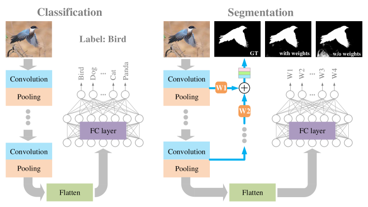
Figure 1: Inspired by the application of fully-connected layers in the classification networks, we replace the prediction of categories with the prediction of weights of features to be fused. The network regulated by weights has a better performance.

Most of the existing methods fuse multi-level features directly without considering the contribution ratio of the fused features to the final output. Therefore, for the first issue, we propose a perception-and-regulation (PR) block to optimize the FPN structure from the perspective of global perception and local feature fusion fine-tuning. Global perception helps to provide accurate semantic information and make better weight regulation, and local feature fusion fine-tuning helps to enhance useful information and suppress invalid information. The perception part of the PR block realizes global perception, which adopts the deepest feature with the largest receptive field as the input. The regulation part of the PR block realizes local feature fusion fine-tuning, which adopts a weighted method to optimize the feature fusion process.

For the second issue, [27][23][28] use atrous convolution to expand the perception range. The too-large atrous ratio will make the information at independent sampling points discontinuous, which is not conducive to the continuity of spatial information in detail. Therefore, the convolution combination of multiple atrous rates is widely adopted [23][28][29] to make the network have the ability to organize a wide space scene and scrutinize highly detailed objects. To solve this problem, we propose our solution, the imitating eye observation module (IEO), to better balance the two abilities.

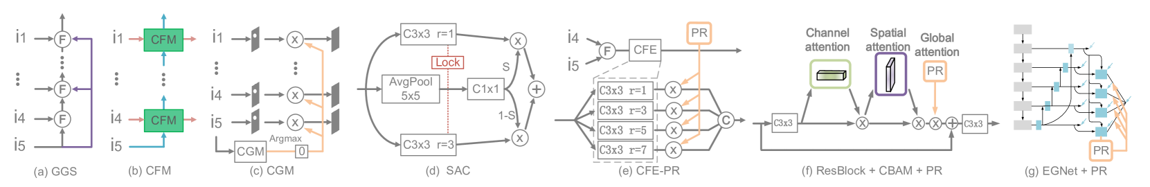
Figure 2: Related module diagrams and the application of PR block in CFE, CBAM, and EGNet. (a) Simplified global guidance structure(GGS) [25] [24]. (b) Cross feature module (CFM) of  [21] (a) (b) is used for semantic information enhancement. (c) Classification-guided module (CGM) of Unet3+ [30] is used to judge whether it is noise or organ. (d) Switchable trous revolution (SAC) [29] is helpful to detect objects of different scales. (e) Context-aware feature extraction module [23] with PR block (f) Convolutional block attention module (CBAM) [31] with PR block (g) Simplified structure of EGNet [22] with PR block.

A partition search strategy is adopted in IEO to effectively alleviate the negative impact of a too-large atrous ratio. The adoption of the PR block enables the IEO module to further balance different types of features in IEO, which helps to further improve network performance.

Inspired by squeeze-and-excitation (SE) block [32] and the classification network, we design a global attention unit called perception-and-regulation (PR) block to regulate the network automatically and achieve the best feature fusion effect. Our goal is to improve the feature fusion effect by explicitly modeling the interdependencies between features to be fused. To achieve this, we design a mechanism that helps the network to recalibrate the feature fusion process, through which it can learn to use global information to adaptively adjust the weights of the features to be fused. In addition, we design an imitating human eye observation module (IEO) to organize a broad spatial scene and have the ability to scrutinize highly detailed objects. Our contributions are summarized as follows:

• We propose a perception-and-regulation (PR) block to help the network understand the global information and assign the feature weights uniformly to realize the spontaneous and adaptive global feature regulation.

• An imitating human eye observation module (IEO) is proposed to help the network have the ability to organize a wide space scene and scrutinize highly detailed objects. PR block balances and optimizes these two abilities.

• Sufficient experiments conducted on 5 SOD datasets demonstrate that the proposed method outperforms 22 state-of-the-art SOD methods in terms of eight metrics. In addition, ablation experiments on several modules and networks prove the universality of our PR block.

II Related work

II-A Salient object detection

Early salient object detection methods are based on hand-crafted features [33][34][35][36][37][38][39][40] and intrinsic cues without a deep hierarchical structure. With the development of deep learning, the deep features with rich contextual information make a great breakthrough in the field of salient object detection. As a landmark algorithm, fully convolutional networks (FCN) [17] creatively removes the fully-connected layer to predict the semantic label for each pixel. Then the U-shape based structures represented by U-net [18] and feature pyramid network (FPN) [19] has gradually become the mainstream structure by integrating all levels of features layer by layer. Based on this structure, scholars have explored more abundant multi-layer feature blending methods to help feature expression effectively. Among them, the global guidance structure (GGS) represented by [20][25][24] has gradually become a common method to strengthen semantic information.

Our Perception-and-Regulation (PR) network is based on GSS to regulate the network spontaneously and adaptively. It is worth noting that, in contrast to FCN abandoning the fully-connected layer (FC), our network mainly relies on the FC layer in the classification network to perceive the size and shape of objects. Then the weights of the features to be fused are evaluated according to the semantic information obtained from the FC layer, as shown in Fig.1.

II-B Semantic information reinforcement

Scholars have proposed various methods to transmit global information of high-level features to the shallow layers to help the network get detail information and accurately locate the objects. For example, Hou et al. [20] proposed short connections to help shallower side-output layers get semantic information more directly. Zhao et al. [22] used the highest-level features to help the edge features (shallow layer) of explicit modeling to filter out useless edge details. Zhao et al. [23] designed a spatial attention module where context-aware high-level features are added to help the location information transfer to the shallow layer. Liu et al. [24] introduced a global guidance module (GGM) to explicitly make shallower layers be aware of the locations of the objects. Global context flow module in  [25] solved the issue of dilution in the process of high-level feature transmission, which is similar to GGM.

The global guidance idea of [25] [24] can be simplified to GGS structure in Fig. 2 (a) and the structure can effectively solve the problem that semantic information is diluted in the process of feature transfer of FPN structure or U-net structure [18]. Even if these structural designs are based on the subjective experience and repeated attempts [20] of excellent scholars, the rigid feature fusion process does not consider the relationship between different features to be fused and the highest level features. The GGS-PR structure of Fig. 3 uses PR block to further slightly regulate and optimize the network. Wei et al. [21] designed a cross feature module (CFM) to select features with rich semantic information to transfer to

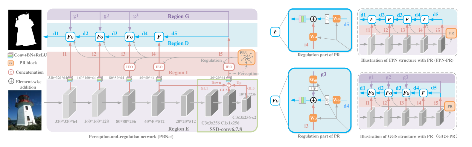
Figure 3: Perception-and-regulation network (PRNet). On the right side of the picture are the applications of PR block in FPN structure and GGS structure. The middle part of the picture shows the regulation part of PR (F-PR and F_G-PR). Besides, F in the GGS structure is not regulated by PR. On the left side of the picture, we add SSD structure and IEO modules to GGS-PR to get the final network PRNet. i1, i2, i3, i4, i5 in region I are the interlayer features. d1, d2, d3, d4, d5 in region D are the decoder features. g1, g2, g3 in region G are global guidance features. The gray dotted arrow represents the input feature of the perception part of PR block. The gray solid arrows in region I represent the regulation of the output weights of the PR block on each feature fusion process.

the shallower layer and let the features with details enter the next cycle as shown in Fig. 2 (b). CFM can be understood as strengthening the transmission of semantic information in FPN structure. Our PR block does the same work, but the way of strengthening semantic features is more flexible and adaptive as shown in the FPN-PR of Fig. 3.

II-C Attention mechanisms

In the classification task, Hu et al. [32] improves the quality of feature representation greatly by establishing the interdependencies between the channels of its convolutional features. Correspondingly, Woo et al. [41][31] use the spatial attention map generated by utilizing the inter-spatial relationship of features with the channel attention map to help the network learn ’where’ is an informative part and ’what’ is meaningful on the spatial and channel axis respectively. Some SOD methods adopt attention mechanism [42][43][44][23]. Wang et al. [45] design the pyramid attention module to make the network pay more attention to important regions and multi-scale information. As a special attention mechanism, the gated mechanism is widely used by long short term memory (LSTM) and gated recurrent unit (GRU), which play an important role in SOD algorithms [46][47][48]. Some segmentation algorithms [49][50][51] use the gated mechanism to adjust the network. CGM of Unet3+ [30] can be regarded as the extreme case of the gated mechanism, because the weights of controlled features are set to 0 or 1 via argmax (Fig.2(c)), which helps to determine whether the target is an organ or noise.

Inspired by SENet [32] and the classification network, we design a PR block for global regulation which can be regarded as a macro global attention mechanism. [32] adaptively recalibrates channel-wise features at the micro level, while PR block recalibrates different types of features of the whole network at the macro level. Different from the existing methods of the gated network, all the features to be fused are regulated in our network and the perception part is located in the position with rich semantic information, which helps to analyze the size and shape of the object accurately and uniformly. In addition, inspired by SAC of [29] (Fig.2(d)), we use softmax, which is commonly used in classification networks, to add constraints to the regulation part of the PR block.

Some algorithms [23][27][29][51][28] use the atrous convolution to expand the receptive range to better observe the object. The disadvantage of atrous convolution with a large atrous ratio is that the information given by spatial continuity may be lost (such as edges) and it is not conducive to the segmentation of small objects. We design a special spatial attention mechanism to compensate for this shortcoming by imitating foveal vision and peripheral vision.

III Perception-and-Regulation Block

The Perception-and-Regulation (PR) block is a computational unit with semantic perception and global regulation capability. The PR block serves the feature level weight regulation of our final network PRNet, as shown in the network structure on the left side of Fig.3. Besides, it can also be used in many network structures or modules.

Inspired by SENet [32] and the classification network, we design a PR block to make the fusion process of different types of features adaptively adjust according to the overall need of weight regulation. SE block focuses on features and adaptively recalibrates features at the channel level, while our PR block focuses on the entire network and recalibrates the entire network at the feature level. Therefore, PR block can be considered as a macro version of SE block.

In addition, FCN [17] adapts classification networks (AlexNet [52], VGG net [53] and GoogLeNet  [54]) into fully convolution networks by replacing the fully-connected (FC) layer with convolution layers to achieve semantic segmentation. On the contrary, we make full use of the perception and understanding ability of the FC layer to make adaptive regulation for the whole network. In Sec.3.1, we discuss three perception strategies in detail for the perception part of the PR block. PR block solves the first issue of how to regulate different types of features to complete better segmentation

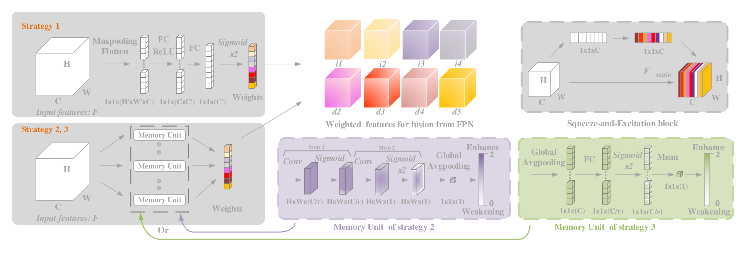
Figure 4: Three perception strategies for the perception-and-regulation block. Strategy 1 uses the fully-connected layer of classification networks to evaluate the weights of the features to be fused. Strategy 2,3 generate feature weights independently for each feature to be fused according to the highest level feature. The dimension change of the weight of strategy 2 is (HxWxC)-(HxWx1)-(1x1x1). The process of strategy 3 is (HxWxC)-(1x1xC)-(1x1x1). The features i1, i2, i3, i4, d2, d3, d4, d5 to be regulated come from the interlayer region (Region I) and decoder region (Region D) of FPN, which correspond to the upper right corner of Fig.3. For the convenience of comparison, we show the SE block in the upper right corner [32].

from the perspective of the overall need for weight regulation. PR block has a better regulation effect on the fusion process of features with large differences. The differences of features here refer to different levels of features (FPN GGS), the features produced by atrous convolution or normal convolution (CFE), the original features or attention features in the residual structure of the attention module (CBAM).

III-A Perception: Semantic Information Embedding

In the perception part of the PR block, three semantic information embedding methods are designed (Fig.4) according to the idea of SENet for global information embedding. In order to introduce our idea clearly, we annotate the features in FPN-PR in the upper right corner of Fig.3.

Strategy 1 in Fig.4 uses the FC layer to perceive the size and shape of the objects. The output of the FC layer of the classification network is the category of the predicted object, while our output results are the weights of the features to be fused. The weights are adjusted adaptively according to the characteristics of the objects. Features regulated by weights are represented by the color of the corresponding weight. Unlike the feature weighting of the SE block for a single channel (Fig.4), the PR block regulates the whole features. The perception part of strategy 1 is set at the location of high-level features (i5) with rich semantic information. Max-pooling is used to reduce the size of the feature $\mathbf{F}$$\in$$\mathbb{R}^{H\times W\times C}$. Then the feature $\mathbf{F_{m}}$$\in$$\mathbb{R}^{H^{{}^{\prime}}\times W^{{}^{\prime}}\times C}$ after pooling is transformed into a one-dimensional vector $\mathbf{F_{f}}$$\in$$\mathbb{R}^{1\times 1\times(H^{{}^{\prime}}\times W^{{}^{\prime}}\times C)}$ by flatten operation. We use a multi-layer perceptron (MLP) [41] with one hidden layer to enhance the perception ability of the network. To save a parameter overhead, the hidden activation size is set to $\mathbb{R}^{1\times 1\times(C\times C^{{}^{\prime}})}$. C${}^{{}^{\prime}}$ is the number of features that need to be regulated and it is eight for the FPN structure in Fig.4. The output layer size is $\mathbb{R}^{1\times 1\times(C^{{}^{\prime}})}$. The activation function of the output layer replaces ReLU with sigmoid and the final results are multiplied by 2 to show whether the features are enhanced or suppressed. In short, the perception part (P_FC) is computed as:

$$\mathbf{P}_{FC}=2*(MLP_{S}(Flatten((MaxPool(\mathbf{F}))))).$$ (1)

The activation function of $MLP_{S}$ output layer is element-wise sigmoid.

Due to the dense connection of FC layers, the final weights of strategy 1 have a strong correlation. In order to explain the perception part of the PR block more clearly, we provide two other spatial dimension (S) and channel dimension (C) perception design. Different from strategy 1, we design multiple independent memory units (MU) for strategy 2,3 (Fig.4) to better illustrate the mapping relationship. The function of MU is to establish the mapping relationship between the shape and size of input features $\mathbf{F}$ and the weight of regulated features. The number of MU is determined by the number of features that need to be regulated. In the MU of strategy 2 , we use two convolution operations to gradually reduce the channel dimension of input features to 1. Here we refer to the design of spatial attention map [41][31]. r is the reduction ratio. The purpose of adding convolution here is to get the output weight according to the input features, and it can be understood that the convolutions change the average gray value of the input features. The weight is equal to the average of the output feature (channel is 1). We change the activation function to sigmoid to enhance the nonlinearity of the output and multiply the final result by 2. In short, the perception part (P_S) is computed as:

$$\mathbf{P}_{S}=G(2*C_{S}(C_{S}(\mathbf{F}))),$$ (2)

where $C_{S}(\cdot)$ is the convolution operation using the element-wise sigmoid function and $G(\cdot)$ is th global average pooling.

For the MU of strategy 3, we use global average pooling to reduce the input feature to one dimension. Then we use the fully-connected layer to reduce the channel to $C/r$. After sigmoid and average operation, the final weight is obtained. The perception part (P_C) is computed as:

$$\mathbf{P}_{C}=Avg(2*FC_{S}(G(\mathbf{F}))),$$ (3)

where $FC_{S}(\cdot)$ is the fully-connected layer and the activation function of the output layer is sigmoid. $Avg(\cdot)$ is the average operation of the one-dimensional vector.

III-B Regulation: Adaptive Recalibration

The accurate location information of high-level features in FPN structure is diluted in the process of multiple fusion [25]. This is because element-wise addition or concatenation operations do not treat the weights of the features to be fused differently. Most of the current algorithms focus on changing the network structure [25][22][24][20] or module [21][45] to enhance semantic information, while the PR network focuses on the regulation of network and can greatly improve the performance of simple network structure. The PR network uses a PR block for global regulation. It builds a bridge between the features to be fused and the semantic information made by the fully-connected layer. The semantic information is expressed in the form of weight.

III-B1 Basic Structural Analysis (FPN-PR and GGS-PR)

Both [24] and [25] use the global guidance method to enhance the semantic information of the shallow features of the network. We add a global guidance structure to the FPN to imitate this process, as shown in Fig.2 (a). The global guidance structure can be considered as a simplified version of  [20][24][25]. The location features are directly added to the shallow features to enhance the ability of salient object location. There is still room for improvement. We add PR block to both FPN and GGS structures (Fig.3) for further slight regulation. [21] proposes a CFM module to help the output features with high-level features (Fig.2 (b) blue arrow) as the main components to transfer to the shallow layer. This scheme is not flexible enough because the structure of CFM is fixed. While the perception part of the PR block helps us to adaptively recalibrate the weight of each feature in the whole network according to the characteristics of the object to achieve better segmentation.

Fig.3 shows the realization of perception and regulation of PR block. In order to simplify the network and reduce the amount of computation, we use convolution (convolution, batch normalization, ReLU) to unify the output features of the encoder to 64 channels. FPN-PR and GGS-PR on the right side of Fig.3 do not show this detail. Taking FPN-PR with perception strategy 2 as an example, eight memory units are used to perceive the input feature and evaluate the weights of interlayer features (i1, i2, i3, i4, i5) and decoder features (d1, d2, d3, d4, d5). The gray dotted arrow represents the input feature $\mathbf{F}$ of the perception part. The gray solid arrows represent the regulation of the eight output weights of the PR block on each feature to be fused. The only difference from the traditional FPN structure is that PR block weights these features. The features (g1, g2, g3) in the purple region G are global guidance features. It is worth noting that we only weighted the three feature fusion process of GGS to explore the influence of PR block on the global guidance. In short, the FPN-PR and GGS-PR are computed as:

$$d_{j-1}^{FPN} =C(W_{i_{j-1}}*i_{j-1}+U(W_{d_{j}}*d_{j})),$$ (4)

$$d_{j-1}^{GGS} =C(W_{i_{j-1}}*i_{j-1}+U(W_{d_{j}}*d_{j})+U(W_{g_{j-1}}*d_{j-1})),$$ (5)

where $C(\cdot)$ refers to the convolution operation. $W$ is the weight. $U(\cdot)$ is upsampling.

In order to make the perception part of PR block have a better perception effect on different scale objects, we adopt the partial encoder design of SSD algorithm [55], as shown in the left part of Fig.3. The advantage of SSD is that it can detect objects on multiple scales. We use its 6,7,8 layer structure and combine 4,7,8 layer features with concatenation to realize multi-layer perception.

III-B2 Exemplars (CFE-PR, CBAM-PR and EGNet-PR)

In order to verify the universality of PR block, we apply it to context-aware feature extraction module (CFE) in Fig.2 (e) [23] and CBAM module in Fig.2 (f) [31]. The features to be fused in FPN and GGS structures are features of different scales and depths, while the features to be fused in CFE-PR modules have different receptive fields.

Different from [23], there are all 3x3 convolution in CFE of this paper and their dilation rates are 1,3,5,7 respectively. CFE is used in the feature i3, i4 and i5 position (follow [23]) of basic FPN structure to enhance the output feature and PR block is used for internal regulation as shown in Fig.2 (e).

As complementary attention modules, channel-wise attention and spatial attention are used to calibrate features at the spatial and channel levels and they can learn ’what’ and ’where’ to attend in the channel and spatial axes respectively [32][41][31]. PR block can be considered as the third type of attention, which focuses on the influence of the whole feature on the network (FPN, GGS) or module(CFE, CBAM). The perception part of the PR block analyzes the global context information of high-level features, and strengthens or weakens the features to be fused from the perspective of the global needs of the network. So we call it global attention in Fig.2 (f). We use PR block with channel attention and spatial attention to further optimize the attention mechanism. The regulation part of the PR block is added to the attention branch of CBAM in Fig. 2 (f) and five CBAM-PR modules are added to i1, i2, i3, i4, i5 positions of the basic FPN structure.

We also added PR block to the final output position of EGNet [22] for perception and regulation, and the final result was further improved. Fig.2 (g) is a simplified structure diagram of EGNet, and we added PR block in its final output location (FPN structure). Line 11-16 of Tab.I proves the effect of PR block in the above modules and networks.

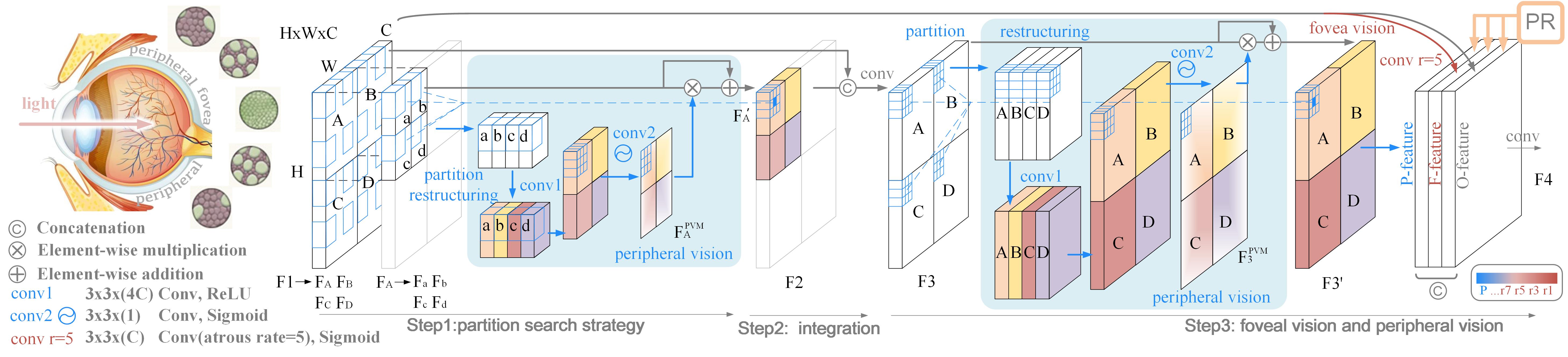
Figure 5: Imitating human eye observation module. The blue area is the peripheral vision module, which is applied twice in steps 1, 3 to make the peripheral vision feature quickly obtain the global receptive field. Under the regulation of PR block, peripheral vision feature, fovea vision feature, and original feature are fused.

IV Imitating Eye Observation Module

The purpose of the imitating human eye observation module (IEO) is to quickly and accurately find and locate salient objects. IEO uses a partition search strategy (Fig.5 step1) to enable the network to focus on the analysis of local areas. Then it uses integration operation (Fig.5 step2) to associate the local feature analysis results with global information. Inspired by human perception of foveal vision and peripheral vision [56], we propose a peripheral vision module (PVM) (Fig.5 blue region) to cooperate with the foveal vision to achieve accurate understanding of the salient objects in step3. The peripheral vision analysis strategy of PVM is applied in both the regional integration step1 and the global search (step3). Step2 is a bridge to make the perception range of peripheral vision wider.

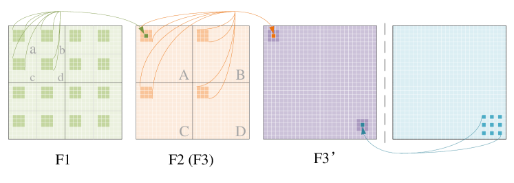
Figure 6: The receptive field of features in peripheral vision module (PVM). The green, orange, and purple squares represent the features F1, F2(F3), and F3’ in Fig.5, respectively. The receptive fields of the green pixel in F2 and the orange pixel in F3 ’are indicated by the guide arrows respectively. The receptive field of the orange pixel in F3’ can cover the dark green areas in F1. The atrous convolution (blue square on the far right) is used to compare with PVM.

In step 1, we divide the input feature $\mathbf{F1}$ into four regions in the spatial dimension ($Par_{S}$) and analyze each region separately with PVM. This mimics the human partition search strategy, which helps to find objects that are not in the center of view. In addition, this operation also helps to form the global receptive field (we will explain it in detail in step 3). Because the sub-regions $F_{A},F_{B},F_{C},F_{D}$ of $\mathbf{F1}$ are partitioned again and then they all pass through the PVM module, we only show the implementation details of $F_{A}$ in Fig.5 step1 and Eq.7-10. The features $F_{a},F_{b},F_{c},F_{d}$ obtained by partitioning $F_{A}$ in spatial dimension ($Par_{s}$) are reorganized in channel dimension ($Cat_{c}$) in Eq.8.

$$F_{A},F_{B},F_{C},F_{D}=Par_{s}(\mathbf{F1}),$$ (6)

$$F_{a},F_{b},F_{b},F_{d}=Par_{s}(F_{A}),$$ (7)

$$F_{A}^{PVM}=C^{2}(Cat_{s}(Par_{c}(C^{1}(Cat_{c}(F_{a},F_{b},F_{b},F_{d}))))),$$ (8)

$$F_{A}^{{}^{\prime}}=F_{A}+F_{A}*F_{A}^{PVM},$$ (9)

where $Par_{s}(\cdot)$, $Par_{c}(\cdot)$, $Cat_{s}(\cdot)$, $Cat_{c}(\cdot)$ refer to spatial dimension partition, channel dimension partition, spatial dimension concatenation, channel dimension concatenation. $C^{1}(\cdot)\in\mathbb{R}^{4C}$ is 3x3 convolution 1 in PVM and activated with ReLU. $C^{2}_{S}(\cdot)\in\mathbb{R}^{1}$ is 3x3 convolution 2 in PVM and activated with sigmoid.

In step 2, we merge the results of partition search (Eq.10) in spatial dimension to get $\mathbf{F2}$ and then use concatenation operation to merge $\mathbf{F1}$, $\mathbf{F2}$ in channel dimension. Step 2 strengthens the association between the region search feature and the original feature.

$$\mathbf{F2}=Cat_{s}(F_{A}^{{}^{\prime}},F_{B}^{{}^{\prime}},F_{C}^{{}^{\prime}},F_{D}^{{}^{\prime}}),$$ (10)

$$\mathbf{F3}=C(Cat_{c}(\mathbf{F1},\mathbf{F2})),$$ (11)

where $C(\cdot)$ $\in\mathbb{R}^{C}$ .

In step 3, we do the peripheral visual perception of $\mathbf{F3}$ again. This process is the same as the previous Eq.7-9. PVM can be considered as a special attention mechanism. It expands the receptive field by comparing the features of corresponding positions in other partitions and then corrects the original features in spatial dimension (F1$\rightarrow$F2 in Fig.6). Eq.9 shows the combination of attention branch and primitive branch [31][41]. PVM can also be considered as a special atrous convolution and has only four sampling points and a very large atrous rate (Fig.6 F3$\rightarrow$F3${}^{{}^{\prime}}$). The PVM here needs to be used for the feature of a large receptive field, otherwise, the spatial information discontinuity caused by a large atrous rate will appear. The problem can be solved by partitioning and stacking PVMs (F1$\rightarrow$F2$\rightarrow$F3). The partition search strategy allows our IEO module to be used for features of the smaller receptive field, which overcomes the limitation of the global perception strategy in [57]. If we want to use the IEO for more shallow features, we can further decompose the features F_A, F_B, F_C and F_D (left side of Fig.5) into smaller sub-regions for partition search and integration before step1 and step2. To keep the network simple, we only used partitioning and integration once in IEO, and let IEOs be used for features i3, i4, i5 in PRNet of Fig.3.

The disadvantage of atrous convolution with a large atrous ratio is that the information given by spatial continuity may be lost (such as edges). Because the sampling points of atrous convolution are too scattered and the information of a single sampling point is not continuous enough. This is the same as the human eye can’t pay attention to the details of objects if there is only peripheral vision. The human eye diagram on the left of Fig. 5 shows the foveal vision cells and peripheral vision cells. Foveal visual cells are rich and concentrated, and they can observe the details of the object. The peripheral visual cells are sparse and widely distributed, and they can organize a broad space scene [58][59]. They are like convolutions of different atrous rates. How to balance these two capabilities is the purpose of IEO module design.

The dark orange dots in F3 of Fig.6 can be regarded as four groups of sampling points of PVM. One sampling point of PVM consists of 9 points (3x3 Conv). Therefore, PVM has both a large atrous rate and detail observation ability. It is worth noting that the 3x3 convolution here can also use atrous convolution with a small atrous rate. For simplicity, we use normal convolution here. The receptive field of the dark orange pixel in F3${}^{{}^{\prime}}$ can cover the dark green areas in F1. The receptive field of F3${}^{{}^{\prime}}$ is global. In addition, we add the fovea vision feature (Fig.5 the red arrow) to cooperate with the P-feature. In the last stage of step 3, we use concatenation operation to merge the original feature, fovea vision feature (r=5), and peripheral vision feature. Finally, we use PR block to balance the relationship among the three types of features.

$$\mathbf{F3^{{}^{\prime}}}=PVM(\mathbf{F3}),$$ (12)

$$W_{1}^{{}^{\prime}},W_{2}^{{}^{\prime}},W_{3}^{{}^{\prime}}=\frac{3*e^{W_{1}}}{\sum_{j=1}^{3}e^{W_{j}}},\frac{3*e^{W_{2}}}{\sum_{j=1}^{3}e^{W_{j}}},\frac{3*e^{W_{3}}}{\sum_{j=1}^{3}e^{W_{j}}},$$ (13)

$$\mathbf{F4}=Cat_{c}(W_{1}^{{}^{\prime}}*\mathbf{F3^{{}^{\prime}}},W_{2}^{{}^{\prime}}*C^{r=5}(\mathbf{F1}),W_{2}^{{}^{\prime}}*\mathbf{F1}),$$ (14)

where $PVM(\cdot)$ is to repeat Eq.7-9 for $\mathbf{F3}$. $W_{1},W_{2},W_{3}$ are the weight produced by the memory unit. Inspired by the classification network, Eq.13 uses a softmax layer to associate weights. SAC uses a similar approach (1-S) to associate partial weights [29]. The three features regulated are peripheral vision feature, fovea vision feature (an original feature after atrous convolution operation), and original feature. The atrous ratio of the convolution of the foveal vision feature is r = 5, which is designed according to the experimental effect.

V Global-Local Transformer

Because the network structure adopts the GSS structure, the positioning accuracy of the high-level features is very important. We have carried out association analysis on cross-regional features through IEO modules to optimize the semantic information of high-level features. In this section, we propose a global-local transformer module (GL-Former) to further optimize the highest-level features. Traditional transformer networks build long-distance dependencies on different regions of the same layer features. The tokens of the same layer in a traditional transformer have the same receptive field range. The tokens of different layers have different receptive fields. The GL-Former we designed uses tokens with different receptive fields to compare and analyze objects of different sizes and better capture salient objects. As shown at the bottom of Fig.7, the design motivation of GL-Former is visually displayed in the form of pictures.

We add GL-Former to optimize the SSD structure of the backbone in Fig.3. The improved structure is shown in Fig.7, the output features GL1, Gl2, and GL3 are optimized twice by two GL-Former modules. Within GL-Former, we change the structure and input to improve the self-attention mechanism into an interactive attention mechanism. This interactive multi-head attention mechanism can help tokens with different receptive fields interact better. The tokens obtained from deeper features have global perception ability, and the tokens obtained from shallower features can capture local information.

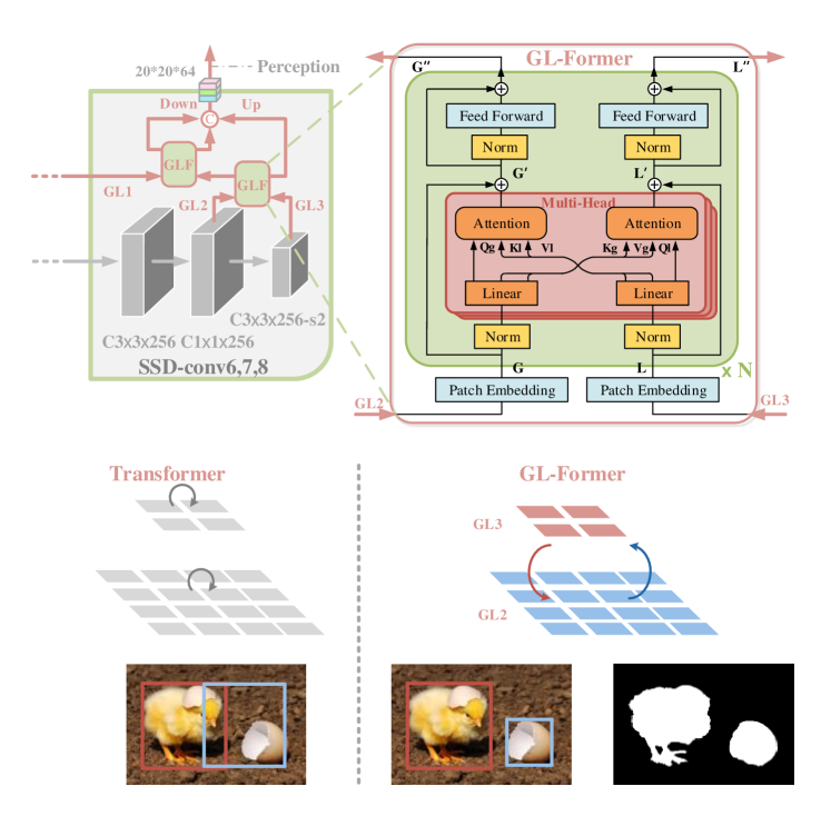
Figure 7: The detailed description of global-local transformer and the application on backbone.

VI Supervision

We use the widely used binary cross entropy (BCE) loss and a consistency-enhanced (CEL) loss [60] to supervise the prediction map, as shown in Eq.15.

$$L=L_{bce}+L_{cel}.$$ (15)

BCE loss is defined as:

$$L_{bce}=-\sum_{(x,y)}[g(x,y)log(p(x,y))+(1-g(x,y))log(1-p(x,y))],$$ (16)

where $p(x,y)\in[0,1]$ is the prediction result of saliency map at $(x,y)$. $g(x,y)\in[0,1]$ is the ground truth label of the pixel $(x,y)$.

CEL loss is a variant of IoU loss, which can measure the similarity of two images from an overall perspective. it is defined as:

$$L_{cel}=\frac{\sum_{(x,y)}[p(x,y)+g(x,y)-2*g(x,y)*p(x,y)]}{\sum_{(x,y)}[g(x,y)+p(x,y)]}.\\$$ (17)

VII Experiment

VII-A Datasets and Evaluation Metrics

We evaluate the proposed architecture on 5 SOD datasets: DUTS [61] with 10,553 training and 5,019 test images, DUT-OMRON [62] with 5,168 images, ECSSD [38] with 1,000 images, PASCAL-S [62] with 850 images, HKU-IS [63] with 4,447 images. We follow the data partition of [60][20] to use 1,447 images of HKU-IS for testing.

In addition, we define a large salient object dataset (L) and a small salient object dataset (S). They are helpful to further analyze the dynamic regulation of PR block when dealing with different scale objects. We select large object images (1270) and small object images (1576) based on the ratio of white pixels in the GT, as shown in Eq.18 and Fig.8. The pictures and ground truth labels are selected from five common test datasets (ECSSD, PASCAL-S, DUT-OMRON, DUTS, HKU-IS). $P_{w}$ is the number of white pixels in the GT and $P_{b}$ is the number of black pixels. $t_{1},t_{2}$ is the threshold. We set $t_{1}$ and $t_{2}$ to 0.38 and 0.03 respectively to obtain dataset L and S.

$$\left\{\begin{array}[]{lr}img\in$L$,&if\frac{P_{w}}{P_{w}+P_{b}}>$t1$\\ img\in$S$,&if\frac{P_{w}}{P_{w}+P_{b}}<$t2$.\end{array}\right.$$ (18)

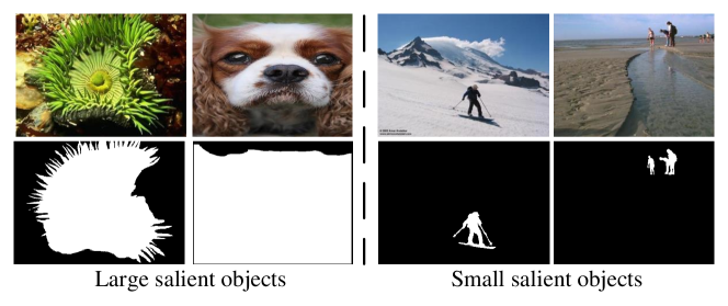
Figure 8: On the left are images of a large salient object dataset. On the right are images of a small salient object dataset.

We use six metrics to evaluate the performance of PRNet and other state-of-the-art models. Mean absolute error (MAE) [64] measures the average pixel-level relative error between the prediction and the GT by calculating the mean of the absolute value of the difference. F-measure ($\textbf{F}_{\beta}$) [33] are also widely adopted in previous models [22][20]. $F_{\beta}$ is the weighted harmonic mean of Precision and Recall and $\beta^{2}$ is usually set to 0.3. The maximal $F_{\beta}$ values are calculated from PR curves, represented as $\textbf{F}_{max}$. An adaptive threshold (twice the mean value of the prediction) is adapted to calculate $\textbf{F}_{avg}$. Weighted F-measure ($\textbf{F}^{w}_{\beta}$) is a measure of completeness for improving F-measure [65]. Structural similarity measure ($\textbf{S}_{\alpha},\alpha=0.5$) [66] and E-measure ($\textbf{E}_{m}$) [67] are also useful for quantitative evaluation of saliency maps. Besides, precision-recall (PR) curves are drawn.

VII-B Implementation

We follow [21][60][68] to use DUTS-TR [61] as the training dataset and other above-mentioned datasets are used as testing datasets. In the training phase, we follow [60] to use random horizontal flipping, random color jittering, and random rotating as data augmentation techniques to prevent the over-fitting problem. PRNet is trained for 40 epochs on an NVIDIA RTX 2080Ti GPU. Batchsize is set to 4. VGG-16, pre-trained on the ImageNet dataset, is used as the backbone network. The parameters for the rest of PRNet are initialized by the default setting of PyTorch. Our model adopts the stochastic gradient descent (SGD) optimizer with a momentum of 0.9, a weight decay of 0.0005, and an initial learning rate of 0.001. ”Poly” strategy [69] (factor is 0.9) is applied. During testing, the input size is set to 320x320.

TABLE I: Ablation experiments on various structures and modules. Because strategy 2 (PR_s) performs best in the final network structure (PRNet), to simplify the experiment, we use strategy PR_s for PR block in the experiments after Line 4.

Model	DUTS-TE				DUT-OMRON
	F${}^{w}_{\beta}$	Em	Sm	MAE	F${}^{w}_{\beta}$	Em	Sm	MAE
1.FPN	.725	.859	.842	.057	.629	.813	.780	.078
2.FPN(PRFC)	.773	.890	.857	.047	.666	.842	.793	.067
3.FPN(PRC)	.764	.887	.852	.048	.658	.839	.788	.068
4.FPN(PRS)	.762	.883	.853	.048	.655	.836	.788	.069
5.FPN(PRS-fixed)	.735	.866	.840	.053	.617	.810	.769	.078
6.FPN(GateNet) [51]	.744	.886	.837	.051	.624	.839	.767	.071
7.FPN+AIMs [60]	.768	.884	.860	.047	-	-	-	-
8.FPNssd(PRS)	.774	.889	.861	.047	.675	.839	.802	.067
9.GGS	.751	.880	.845	.051	.641	.828	.777	.073
10.GGS(PRS)	.766	.892	.851	.047	.651	.841	.783	.068
11.FPN+CBAM [31]	.768	.888	.856	.048	.661	.837	.792	.069
12.FPN+CBAM(PRS)	.775	.894	.858	.046	.666	.847	.793	.066
13.FPN+CFE [23]	.793	.896	.867	.044	.688	.849	.805	.062
14.FPN+CFE(PRS)	.798	.902	.869	.043	.700	.856	.812	.060
15.EGNet [22]	.802	.897	.878	.044	.728	.864	.836	.057
16.EGNet(PRS) [22]	.806	.900	.881	.042	.731	.866	.837	.056
17. CFD [21]	.778	.890	.858	.047	.674	.836	.796	.066
18. CFD(PRS) [21]	.790	.891	.861	.044	.681	.842	.799	.062

TABLE II: Ablation experiment of PRNet. Because strategy 2 (PR_s) performs best in the final network structure (PRNet 3rd line), to simplify the experiment, PR_s is used in every step of the ablation experiment. The model in the 6th line is the same as that in the 3rd line, but the loss only uses BCE loss (CEL loss is removed).

Model	DUTS-TE				DUT-OMRON
	F${}^{w}_{\beta}$	Em	Sm	MAE	F${}^{w}_{\beta}$	Em	Sm	MAE
1. GGSssd(PRS)	.755	.877	.859	.050	.660	.837	.801	.069
2. GGSssd(PRS) + IEO	.793	.901	.868	.043	.692	.851	.809	.062
3. GGSssd(PRS) + IEO(PRS)	.802	.908	.872	.041	.698	.857	.812	.059
4. GGSGLF(PRS) + IEO(PRS)	.803	.908	.875	.041	.700	.859	.814	.059
5. GGS(PRS) + IEO(PRS)	.794	.903	.868	.042	.690	.856	.807	.060
6. GGSssd(PRS) + CFE(PRS)	.794	.902	.869	.043	.696	.856	.812	.061
7. w/o CEL	.765	.879	.865	.048	.669	.840	.808	.067

TABLE III: Ablation Experiment of IEO Module. We adjust the location and number of IEO on the basis of PRNet(PR_S). The experiments show that the best location is i3 i4 i5.

Model	DUTS-TE				DUT-OMRON
	F${}^{w}_{\beta}$	Em	Sm	MAE	F${}^{w}_{\beta}$	Em	Sm	MAE
1. IEO in i5	.790	.901	.867	.043	.684	.849	.805	.063
2. IEO in i4, i5	.792	.905	.867	.042	.682	.850	.803	.063
3. IEO in i3, i4, i5	.802	.908	.872	.041	.698	.857	.812	.059
4. IEO in i2, i3, i4, i5	.797	.904	.870	.042	.699	.859	.813	.060
5. IEO in i1, i2, i3, i4, i5	.798	.903	.871	.042	.699	.856	.813	.061

TABLE IV: Comparison of 3 types of perception strategies in PRNet.

Model	DUTS-TE				DUT-OMRON
	F${}^{w}_{\beta}$	Em	Sm	MAE	F${}^{w}_{\beta}$	Em	Sm	MAE
1. PRNet(PRFC)	.794	.904	.868	.042	.690	.852	.807	.062
2. PRNet(PRS)	.802	.908	.872	.041	.698	.857	.812	.059
3. PRNet(PRC)	.792	.902	.868	.043	.686	.851	.806	.062

VII-C Ablation Studies

Ablation analysis of PR block in different structures and modules. Lines 1-4 of Tab.I analyze the effect of PR block with different perception strategies in FPN structure. $PR_{FC},PR_{C},PR_{S}$ are strategy 1,2,3 in Fig.4. The $PR_{FC}$ has the best regulation effect in FPN structure because of its rich parameters and intensive interaction analysis in the fully-connected layer. But in the final network structure (PRNet), $PR_{S}$ is the best (Tab.IV), we will explain this phenomenon in later analysis. In order to simplify the experiment, we uniformly use the best strategy $PR_{S}$ in the final network to carry out the comparison experiments and the ablation experiment in Tab.I, Tab.II and Tab.III. Line 6 of Tab.I is the gate strategy provided by the GateNet [51], and its effect is not as good as the PR block of global perception and regulation. It is worth noting that line 7 of Tab.I is the AIMs module of MINet [60]. AIM has a more complex interaction structure than PR block, but the regulation effect of PR block is better. Line 8 verify the effect of the multi-level perception strategy in the FPN structure. FPN_ssd(PR_S) means that FPN-PR uses the encoder structure shown in the left side of Fig. 3. Line 9-18 verify the improvement of PR block to GGS structure (the lower right corner of Fig.3), CFE module (Fig.2 (e)), CBAM module (Fig.2 (f)), EGNet network (Fig.2 (g)) and CFD decoder (Fig.2 (b)).

Ablation analysis of the PRNet. Tab.II shows the ablation experiment of PRNet (Fig.3). The baseline is GGS$ssd$(PR_S). IEO improves the network performance greatly in line 2, but the allocation of foveal vision feature and peripheral vision feature is not balanced. The performance of IEO is further improved after being regulated by PR block (line 3). The right side of Fig. 5 shows how the weights obtained by the perception part regulate the features of IEO. Lines 3 and 4 show the effect of multi-level perception. The experiment in the 5th line replaces the IEO-PR module in the 3rd line with the CFE-PR module (Fig.2 (e)), which proves the effectiveness of the IEO-PR module. The model of the experiment in the 6th line is the same as that in the 3rd line, but the experiment in the 6th line is only supervised by BCE loss (CEL loss is removed). The 3rd and 6th experiments show the effect of CEL loss.

It is worth noting that, as shown in Fig.3, the IEO and CFE modules in Tab.II are placed in i3, i4, and i5 positions, which follows the setting of  [23]. The peripheral vision module in the IEO module has a large void rate, so it is better to use it for high-level features with a larger receptive field. Experiments in Tab.III also show that this scheme is the best for IEO-PR module. Besides, reducing the number of IEO modules is conducive to simplify the model and improving the speed.

Perception strategy analysis. Lines 1,2,3,4 of Tab.I show that strategy 1 (PR_FC) is the best in simple structures (FPN). While strategy 2 (PR_S) performs best in complex structures (PRNet) as shown in Tab.IV.

The fully-connected layers in PR_FC that are inspired by the classification network make the weights coupled and correlation strong as shown in Fig.4. In addition, there are many parameters in the FC layer, which is also helpful to recalibrate the weights of features with obvious differences in the simple structure (FPN). But for complex network PRNet, the difference between the features to be fused becomes smaller. Take the feature fusion process F_G on the far right of PRNet (Fig.3) as an example, because d4 is the fusion feature of g2 (d5) and i4, the difference between g2 and d4 is reduced. Fully-connected layers in strategy 1 over-interpret the weights, which makes the effect of PR_FC block worse. Fully-connected layers are also used in strategy 3 (PR_C), so it has the same problem. The MU of strategy 3 evaluates each feature weight independently, which is different from the strong coupling in strategy 1. Strategy 3 can be considered as a simplified version of strategy 1 because the parameters of its fully-connected layer are less than strategy 1. Strategy 1 performs better on simple networks (FPN, CFD), and strategy 2 performs better on complex networks (PRNet, EGNet). Besides, we analyze the weights of strategies 1 and 2 in the FPN structure, as shown in Fig.9. We can find that strategy 1 is radical and sensitive, while strategy 2 is conservative and restricted. These characteristics result in the performance differences between the two strategies in simple network structure and complex network structure.

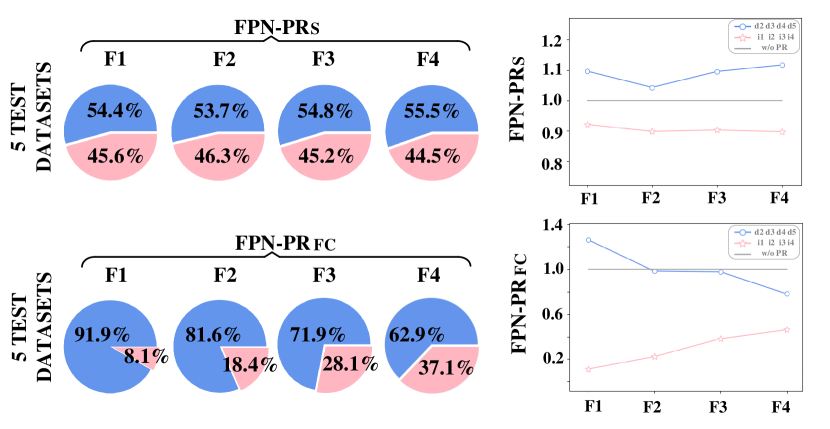
Figure 9: The effect analysis of strategy 1 (PR_FC) and strategy 2 (PR_S) in FPN architecture. The pie chart and line chart show the statistical results of feature weights on five test datasets. The pie chart is presented in the proportion of feature weight. The line chart is presented in the form of concrete numerical value. F1-F5 represent the five feature fusion processes of FPN. F1 represents the feature fusion process of i1 and d2. The blue regions represent the weight ratio of decoder features (d2, d3, d4, d5). The pink regions represent the weight ratio of interlayer features (i1, i2, i3, i4). For the feature definitions of i1 and d2, please refer to FPN-PR in the upper right corner of Fig.3.

PR_S directly uses global average pooling to reduce the spatial dimension (H, W) to (1, 1), which is beneficial for complex networks (PRNet) with little difference in features to be fused. Because there is no fully-connected layer, the final weights are more directly and closely related to the spatial features of salient objects. PR_S can prevent overfitting of the fully-connected layers in strategy 1, 3.

PR block is originally inspired by the classification network. And we find that the paper, Network In Network (NIN) [70], just verifies this phenomenon from the perspective of the classification task. NIN explains the advantages of global average pooling to replace the fully connected layer in detail. According to the above analysis, we can use strategy 1 to regulate the feature fusion process with large feature differences, while strategy 2 can be used for the feature fusion process with small feature differences. In addition, it should be noted that strategy 1 is not suitable for all feature fusion processes. For the case that the difference between the features to be fused is very small, radical weight regulation may have a negative impact.

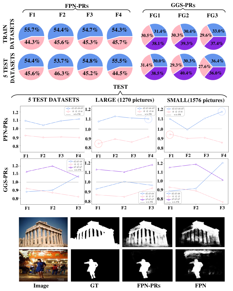
Figure 10: Weight analysis. For FPN-PR_S and GGS-PR_S, we use pie charts and line charts to show the average values of multiple fusion position weights of 5 test datasets and the training dataset. In the line chart, we use 1270 images of large objects and 1576 images of small objects respectively to show how the PR block regulates the network in the segmentation task of objects of different scales.

Feature weight analysis. To further analyze how the PR block works, we show the average weight of each fusion position in the pie chart and line chart in Fig.10. F1-4 and FG1-3 represent multiple regulated points of FPN-PR and GGS-PR (Fig.3). The pie chart shows the results in the training dataset and 5 test datasets. The line chart shows the results of 5 test datasets and the results of 1300 pictures with large objects and 1300 pictures with small objects. The images of large objects and small objects are obtained by setting threshold according to the area ratio of white pixels in GT. Blue, red and purple regions and lines represent decoder features, interlayer features, and global features respectively. The grey line indicates that the weight of the feature without PR block regulation is 1.

We use the dotted circle to indicate the position where the weight of the PR block changes obviously. This change is strongly related to the size of the salient object. It is worth noting that the highest-level features (d5) of small objects are specially enhanced (dotted circle in the small object) to prevent dilution. The lowest-level (i1) features in large objects are sufficiently suppressed to prevent interference. The left side of Fig.10 shows the effect of the PR block. In order to verify that the dynamic regulation of weights is meaningful, we lock the weights in Tab.I line 5. The weights of FPN(PR_S-fixed) is obtained from the average weight of training dataset. Line

TABLE V: Quantitative evaluation. We compare 22 SOD methods on 5 SOD datasets. The maximum and mean F-measure (larger is better), S-measure (larger is better) and MAE (smaller is better) of different salient object detection methods on five benchmark datasets. The best three results are highlighted in ${\color[rgb]{1,0,0}red},{\color[rgb]{.357,.608,.835}blue}$ and ${\color[rgb]{.439,.678,.278}green}$. -V: VGG16 as backbone in the algorithm that provides multiple backbones. *: We compare the PoolNet algorithm that uses only the DUTS-TE dataset for training. -: The author do not provide the test results of the corresponding datasets.

Model	DUTS-TE						DUT-OMRON						HKU-IS						ECSSD						PASCAL-S
	Fmax	Favg	F${}^{w}_{\beta}$	Em	Sm	MAE	Fmax	Favg	F${}^{w}_{\beta}$	Em	Sm	MAE	Fmax	Favg	F${}^{w}_{\beta}$	Em	Sm	MAE	Fmax	Favg	F${}^{w}_{\beta}$	Em	Sm	MAE	Fmax	Favg	F${}^{w}_{\beta}$	Em	Sm	MAE
DCL16	.782	.712	.408	.839	.734	.088	.757	.695	.583	.830	.772	.080	.757	.695	.583	.830	.772	.080	.901	.874	.790	.908	.870	.068	.830	.776	.685	.836	.794	.108
Amulet17	.778	.671	.655	.798	.803	.085	.743	.647	.625	.784	.780	.098	.897	.842	.816	.914	.884	.051	.915	.869	.841	.912	.893	.059	.841	.771	.741	.831	.821	.098
NLDF17	.813	.739	.710	.855	.816	.065	.753	.684	.634	.817	.770	.080	.902	.872	.839	.929	.878	.048	.905	.878	.839	.912	.875	.063	.833	.782	.742	.842	.804	.099
UCF17	.771	.624	.586	.766	.777	.117	.735	.613	.564	.763	.758	.132	.888	.810	.753	.893	.866	.074	.911	.840	.789	.888	.883	.078	.830	.708	.681	.787	.803	.126
MSRNet17	.829	.703	.720	.840	.839	.061	.782	.676	.669	.820	.808	.073	.914	.857	.853	.935	.902	.040	.911	.839	.849	.905	.895	.054	.858	.747	.769	.837	.841	.081
DSS17	.826	.789	.755	.885	.824	.056	.772	.729	.691	.846	.788	.066	.910	.894	.864	.938	.879	.041	.916	.900	.871	.924	.882	.053	.839	.807	.760	.851	.797	.096
BMPM18	.852	.745	.761	.863	.862	.049	.774	.692	.681	.839	.809	.064	.920	.871	.860	.938	.907	.039	.928	.868	.871	.916	.911	.045	.864	.771	.785	.847	.845	.075
RAS18	.831	.751	.740	.864	.839	.059	.787	.713	.695	.849	.814	.062	.913	.871	.843	.931	.887	.045	.921	.889	.857	.922	.893	.056	.838	.787	.738	.837	.795	.104
PAGRN18	.854	.784	.724	.883	.838	.056	.771	.711	.622	.843	.775	.071	.919	.887	.823	.941	.889	.047	.927	.894	.834	.917	.889	.061	.858	.808	.738	.854	.817	.093
C2S18	.811	.717	.717	.847	.831	.062	.759	.682	.663	.828	.799	.072	.898	.851	.834	.928	.886	.047	.911	.865	.854	.915	.896	.053	.857	.775	.777	.850	.840	.080
PoolNet${}_{19}^{*}$	.876	-	-	-	.043	.817	.817	-	-	-	-	.058	.928	-	-	-	-	.035	.936	-	-	-	-	.047	.857	-	-	-	-	.078
AFNet19	.863	.793	.785	.895	.867	.046	.797	.739	.717	.859	.826	.057	.925	.889	.872	.949	.906	.036	.935	.908	.886	.941	.913	.042	.871	.828	.804	.887	.850	.071
MLMSNet19	.852	.745	.761	.863	.862	.049	.774	.692	.681	.839	.809	.064	.920	.871	.860	.938	.907	.039	.928	.868	.871	.916	.911	.045	.864	.771	.785	.847	.845	.075
PAGE19	.838	.777	.769	.886	.854	.052	.792	.736	.722	.860	.825	.062	.920	.884	.868	.948	.904	.036	.931	.906	.886	.943	.912	.042	.859	.817	.792	.879	.840	.078
BANet-V19	.852	.789	.781	.891	.861	.046	.793	.731	.719	.856	.823	.061	.920	.887	.871	.948	.903	.036	.935	.910	.890	.944	.913	.041	.867	.826	.799	.879	.841	.078
HRS19	.843	.793	.746	.889	.829	.051	.762	.708	.645	.842	.772	.066	.913	.892	.854	.938	.883	.042	.920	.902	.859	.923	.883	.054	.852	.809	.748	.850	.801	.090
GATE-V20	.870	.783	.786	.888	.870	.045	.794	.724	.704	.854	.821	.061	.928	.889	.872	.948	.909	.035	.941	.896	.886	.931	.917	.041	.882	.810	.807	.870	.856	.070
ITSD-V20	.877	.798	.814	.893	.877	.042	.807	.745	.734	.858	.829	.063	.926	.891	.882	.947	.907	.035	.939	.875	.897	.918	.914	.040	.884	.787	.824	.857	.858	.068
FCNet20	.829	.795	.757	.887	.822	.045	.717	.676	.618	.795	.745	.066	-	-	-	-	-	-	-	-	-	-	-	-	.857	.830	.802	.882	.830	.068
HVPNet20	.840	.749	.730	.863	.849	.058	.804	.721	.700	.847	.831	.065	.916	.871	.840	.936	.899	.045	.928	.889	.855	.924	.903	.052	.849	.794	.753	.850	.827	.091
CAGNet-V20	.851	.820	.797	.900	.852	.045	.782	.743	.718	.858	.807	.057	.922	.906	.888	.948	.899	.033	.930	.911	.892	.932	.897	.042	.860	.828	.799	.874	.825	.077
SAMNet21	.836	.745	.729	.864	.849	.058	.803	.717	.699	.847	.830	.065	.915	.870	.837	.938	.898	.045	.928	.891	.858	.930	.907	.050	.850	.790	.747	.849	.824	.093
PRNet	.877	.815	.802	.908	.872	.041	.789	.731	.698	.857	.812	.059	.930	.906	.885	.956	.910	.033	.936	.913	.890	.941	.910	.041	.884	.843	.815	.893	.856	.067

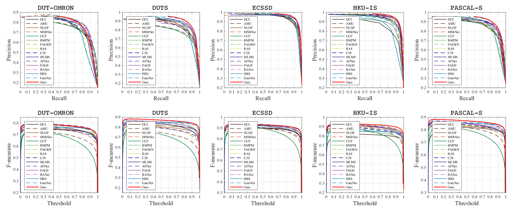
Figure 11: Precision-Recall curves (1st row) and F-measure curves (2nd row) on five common saliency datasets.

1,4,5 show that it is effective to suppress low-level features with fixed weights, but it is better to regulate the weights according to the analysis results of the PR block.

VII-D Comparison with State-of-the-arts

We compare PRNet against 22 SOD state-of-the-art methods, including DCL [71], NLDF [72], MSRNet [73], DSS [20], BMPM [50], RAS [42], PAGRN [43], C2S [74], PAGE [45], BANet [75], AFNet [57], GateNet [51], ITSD [76], FCNet [77], HVPNet [78], CAGNet [79], SAMNet [80], etc.

For fair comparisons, we use all saliency maps provided by the authors or generated by their codes. PoolNet [24] (with StdEdge) adds another dataset (BSDS500) for joint training, which makes the comparison results unfair. So we compare PRNet with PoolNet (with SalEdge, only DUTS-TE dataset) in Tab. V, and the experimental result shows that our algorithm is better. Our PRNet (only 130M) is a simple network, so there is no comparison with EGNet (434M) [22] and MINet (650M) [60] with large parameters.

Quantitative evaluation. Tab. V shows the scores of the proposed model and 22 state-of-the-art saliency detection methods on five widely used datasets and also demonstrates that the perception-and-regulation strategy is successful in making simple networks perform favorably against other algorithms. Moreover, the PR curves by our approach outperform other methods, as shown in Fig. 11.

Qualitative evaluation. Fig. 12 shows the visual examples produced by our model and other models. From the 1st row to the 10th row, the size of the salient object gradually changes from the largest to the smallest. Our algorithm is effective in dealing with multi-scale object detection. The proposed method performs better in various challenging scenarios, including the small object, medium-sized object, and big object. Fig.13 shows the visualization results of the whole process. The difference between the FPN network with a PR block and the FPN network without a PR block is clearly shown. Besides, we provide some failure cases of our algorithm in the supporting document to help future researchers to conduct further analysis.

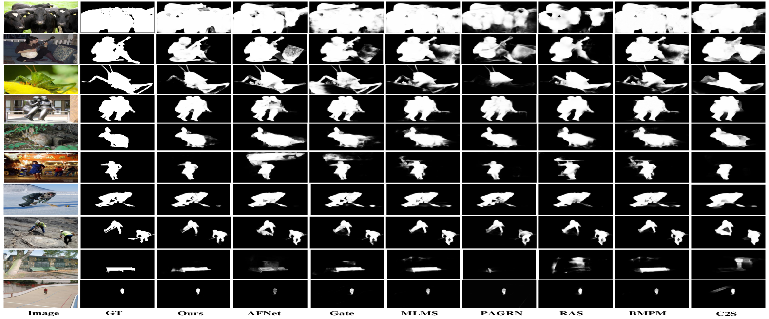
Figure 12: Qualitative comparisons with state-of-the-art algorithms. From top to bottom, the size of salient objects gradually decreases.

Figure 13: Visual analysis of PR block regulation process. We show two examples (more examples can be found in the supporting document). For the feature analysis of the bird, the 1st and 2nd rows are the decoder features d1-d5 of FPN and the decoder features d1-d5 of FPN-PR_FC, respectively. The 3rd row is ground truth, the input image and encoder (VGG-16) features i1-i4. The 1st column is the final output saliency maps of FPN and FPN-PR_FC. In the red box is the feature fusion process of FPN-PR_FC. The gray (encoder), red (interlayer features), and blue (decoder features) arrows correspond to the FPN-PR_FC in the upper right corner of Fig.3. The white font is the result of weight regulated by PR block (PR_FC).

VIII Conclusions

In this paper, we propose a novel framework PRNet for salient object detection. A PR block is designed to help the network understand the global information and assign the feature weights spontaneously and adaptively. To better perceive semantic information and reasonably allocate weight, we propose 3 perception strategies and carry out comparative experiments. Through experiments, we verify the different application scenarios of different strategies. Considering the relationship between local perception and global perception, we propose an IEO module to help the network have the ability to organize a wide space scene and scrutinize highly detailed objects. Sufficient experiments demonstrate that PRNet performs well. In the future, we may expand PRNet to more complex structures, such as recurrent structure networks and multi-modal SOD networks (RGB-T, RGB-D).

References

- [1] W. Wang, Q. Lai, H. Fu, J. Shen, H. Ling, and R. Yang, “Salient object detection in the deep learning era: An in-depth survey,” IEEE Transactions on Pattern Analysis and Machine Intelligence, pp. 1–1, 2021.
- [2] B. Jiang, Z. Zhou, X. Wang, J. Tang, and L. Bin, “cmSalGAN: RGB-D salient object detection with cross-view generative adversarial networks,” IEEE Transactions on Multimedia, 2020.
- [3] D.-P. Fan, T. Li, Z. Lin, G.-P. Ji, D. Zhang, M.-M. Cheng, H. Fu, and J. Shen, “Re-thinking co-salient object detection,” IEEE Transactions on Pattern Analysis and Machine Intelligence, pp. 1–1, 2021.
- [4] D.-P. Fan, Z. Lin, Z. Zhang, M. Zhu, and M.-M. Cheng, “Rethinking rgb-d salient object detection models, data sets, and large-scale benchmarks,” IEEE Transactions on Neural Networks and Learning Systems, vol. 32, no. 5, pp. 2075–2089, 2020.
- [5] J. Zhang, Y. Dai, T. Zhang, M. Harandi, N. Barnes, and R. Hartley, “Learning saliency from single noisy labelling: A robust model fitting perspective,” IEEE Transactions on Pattern Analysis and Machine Intelligence, vol. 43, no. 8, pp. 2866–2873, 2021.
- [6] Q. Chen, K. Fu, Z. Liu, G. Chen, H. Du, B. Qiu, and L. Shao, “EF-Net: A novel enhancement and fusion network for RGB-D saliency detection,” Pattern Recognition, vol. 112, p. 107740, 2021.
- [7] J. Zhang, X. Yu, A. Li, P. Song, B. Liu, and Y. Dai, “Weakly-supervised salient object detection via scribble annotations,” in IEEE Conference on Computer Vision and Pattern Recognition (CVPR), 2020, pp. 12 543–12 552.
- [8] Q. Chen, Z. Liu, Y. Zhang, K. Fu, Q. Zhao, and H. Du, “RGB-D salient object detection via 3d convolutional neural,” in AAAI Conference on Artificial Intelligence (AAAI), 2021.
- [9] J. Zhang, D.-P. Fan, Y. Dai, S. Anwar, F. Saleh, S. Aliakbarian, and N. Barnes, “Uncertainty inspired rgb-d saliency detection,” IEEE Transactions on Pattern Analysis and Machine Intelligence, pp. 1–1, 2021.
- [10] W. Wang, J. Shen, and L. Shao, “Video salient object detection via fully convolutional networks,” IEEE Transactions on Image Processing, vol. 27, no. 1, pp. 38–49, 2018.
- [11] W. Wang, J. Shen, R. Yang, and F. Porikli, “Saliency-aware video object segmentation,” IEEE Transactions on Pattern Analysis and Machine Intelligence, vol. 40, no. 1, pp. 20–33, 2018.
- [12] W. Wang, J. Shen, and H. Ling, “A deep network solution for attention and aesthetics aware photo cropping,” IEEE Transactions on Pattern Analysis and Machine Intelligence, vol. 41, no. 7, pp. 1531–1544, 2019.
- [13] M.-M. Cheng, F.-L. Zhang, N. J. Mitra, X. Huang, and S.-M. Hu, “Repfinder: Finding approximately repeated scene elements for image editing,” ACM Trans. Graph., vol. 29, no. 4, Jul. 2010.
- [14] T. Wang, Y. Piao, H. Lu, X. Li, and L. Zhang, “Deep learning for light field saliency detection,” in IEEE International Conference on Computer Vision (ICCV), 2019, pp. 8837–8847.
- [15] T. Chen, M.-M. Cheng, P. Tan, A. Shamir, and S.-M. Hu, “Sketch2photo: Internet image montage,” ACM Trans. Graph., vol. 28, no. 5, p. 1–10, Dec. 2009.
- [16] V. Mahadevan and N. Vasconcelos, “Saliency-based discriminant tracking,” in IEEE Conference on Computer Vision and Pattern Recognition (CVPR), 2009, pp. 1007–1013.
- [17] J. Long, E. Shelhamer, and T. Darrell, “Fully convolutional networks for semantic segmentation,” in IEEE Conference on Computer Vision and Pattern Recognition (CVPR), 2015, pp. 3431–3440.
- [18] O. Ronneberger, P. Fischer, and T. Brox, “U-net: Convolutional networks for biomedical image segmentation,” in Medical Image Computing and Computer-Assisted Intervention (MICCAI), vol. 9351, 2015, pp. 234–241.
- [19] T.-Y. Lin, P. Dollár, R. Girshick, K. He, B. Hariharan, and S. Belongie, “Feature pyramid networks for object detection,” in IEEE Conference on Computer Vision and Pattern Recognition (CVPR), 2017, pp. 2117–2125.
- [20] Q. Hou, M.-M. Cheng, X. Hu, A. Borji, Z. Tu, and P. H. S. Torr, “Deeply supervised salient object detection with short connections,” IEEE Transactions on Pattern Analysis and Machine Intelligence, vol. 41, no. 4, pp. 815–828, 2019.
- [21] J. Wei, S. Wang, and Q. Huang, “F3Net: Fusion, feedback and focus for salient object detection,” in AAAI Conference on Artificial Intelligence (AAAI), 2020.
- [22] J. Zhao, J.-J. Liu, D.-P. Fan, Y. Cao, J. Yang, and M.-M. Cheng, “Egnet: Edge guidance network for salient object detection,” in IEEE International Conference on Computer Vision (ICCV), 2019, pp. 8778–8787.
- [23] T. Zhao and X. Wu, “Pyramid feature attention network for saliency detection,” in IEEE Conference on Computer Vision and Pattern Recognition (CVPR), 2019, pp. 3080–3089.
- [24] J.-J. Liu, Q. Hou, M.-M. Cheng, J. Feng, and J. Jiang, “A simple pooling-based design for real-time salient object detection,” in IEEE Conference on Computer Vision and Pattern Recognition (CVPR), 2019, pp. 3912–3921.
- [25] Z. Chen, Q. Xu, R. Cong, and Q. Huang, “Global context-aware progressive aggregation network for salient object detection,” in AAAI Conference on Artificial Intelligence (AAAI), 2020, pp. 10 599–10 606.
- [26] S. Yu, B. Zhang, J. Xiao, and E. G. Lim, “Structure-consistent weakly supervised salient object detection with local saliency coherence,” in AAAI Conference on Artificial Intelligence (AAAI), 2021.
- [27] D.-P. Fan, G.-P. Ji, G. Sun, M.-M. Cheng, J. Shen, and L. Shao, “Camouflaged object detection,” in IEEE Conference on Computer Vision and Pattern Recognition (CVPR), 2020, pp. 2774–2784.
- [28] L.-C. Chen, G. Papandreou, I. Kokkinos, K. Murphy, and A. L. Yuille, “Deeplab: Semantic image segmentation with deep convolutional nets, atrous convolution, and fully connected crfs,” IEEE Transactions on Pattern Analysis and Machine Intelligence, vol. 40, no. 4, pp. 834–848, 2018.
- [29] S. Qiao, L. C. Chen, and A. Yuille, “Detectors: Detecting objects with recursive feature pyramid and switchable atrous convolution,” arXiv, 2020.
- [30] H. Huang, L. Lin, R. Tong, H. Hu, Q. Zhang, Y. Iwamoto, X. Han, Y.-W. Chen, and J. Wu, “Unet 3+: A full-scale connected unet for medical image segmentation,” in IEEE International Conference on Acoustics, Speech and Signal Processing (ICASSP), 2020, pp. 1055–1059.
- [31] S. Woo, J. Park, J. Lee, and I. S. Kweon, “CBAM: convolutional block attention module,” in Europeon Conference on Computer Vision (ECCV), vol. 11211, 2018, pp. 3–19.
- [32] J. Hu, L. Shen, S. Albanie, G. Sun, and E. Wu, “Squeeze-and-excitation networks,” IEEE Transactions on Pattern Analysis and Machine Intelligence, vol. 42, no. 8, pp. 2011–2023, 2020.
- [33] R. Achanta, S. Hemami, F. Estrada, and S. Susstrunk, “Frequency-tuned salient region detection,” in IEEE Conference on Computer Vision and Pattern Recognition, 2009, pp. 1597–1604.
- [34] M.-M. Cheng, N. J. Mitra, X. Huang, P. H. S. Torr, and S.-M. Hu, “Global contrast based salient region detection,” IEEE Transactions on Pattern Analysis and Machine Intelligence, vol. 37, no. 3, pp. 569–582, 2015.
- [35] Z. Jiang and L. S. Davis, “Submodular salient region detection,” in IEEE Conference on Computer Vision and Pattern Recognition (CVPR), 2013, pp. 2043–2050.
- [36] D. A. Klein and S. Frintrop, “Center-surround divergence of feature statistics for salient object detection,” in International Conference on Computer Vision (ICCV), 2011, pp. 2214–2219.
- [37] H. Jiang, J. Wang, Z. Yuan, Y. Wu, N. Zheng, and S. Li, “Salient object detection: A discriminative regional feature integration approach,” in IEEE Conference on Computer Vision and Pattern Recognition (CVPR), 2013, pp. 2083–2090.
- [38] Q. Yan, L. Xu, J. Shi, and J. Jia, “Hierarchical saliency detection,” in IEEE Conference on Computer Vision and Pattern Recognition (CVPR), 2013, pp. 1155–1162.
- [39] C. Yang, L. Zhang, H. Lu, X. Ruan, and M.-H. Yang, “Saliency detection via graph-based manifold ranking,” in IEEE Conference on Computer Vision and Pattern Recognition (CVPR), 2013, pp. 3166–3173.
- [40] W. Wang, J. Shen, L. Shao, and F. Porikli, “Correspondence driven saliency transfer,” IEEE Transactions on Image Processing, vol. 25, no. 11, pp. 5025–5034, 2016.
- [41] J. Park, S. Woo, J. Lee, and I. S. Kweon, “BAM: bottleneck attention module,” in British Machine Vision Conference (BMVC), 2018, p. 147.
- [42] S. Chen, X. Tan, B. Wang, H. Lu, X. Hu, and Y. Fu, “Reverse attention based residual network for salient object detection,” IEEE Transactions on Image Processing, vol. 29, pp. 3763–3776, 2020.
- [43] X. Zhang, T. Wang, J. Qi, H. Lu, and G. Wang, “Progressive attention guided recurrent network for salient object detection,” in IEEE Conference on Computer Vision and Pattern Recognition (CVPR), 2018, pp. 714–722.
- [44] Z. Wu, L. Su, and Q. Huang, “Cascaded partial decoder for fast and accurate salient object detection,” in IEEE Conference on Computer Vision and Pattern Recognition (CVPR), 2019, pp. 3902–3911.
- [45] W. Wang, S. Zhao, J. Shen, S. C. H. Hoi, and A. Borji, “Salient object detection with pyramid attention and salient edges,” in IEEE Conference on Computer Vision and Pattern Recognition (CVPR), 2019, pp. 1448–1457.
- [46] W. Wang, J. Shen, M.-M. Cheng, and L. Shao, “An iterative and cooperative top-down and bottom-up inference network for salient object detection,” in IEEE Conference on Computer Vision and Pattern Recognition (CVPR), 2019, pp. 5961–5970.
- [47] W. Wang, J. Shen, X. Dong, A. Borji, and R. Yang, “Inferring salient objects from human fixations,” IEEE Transactions on Pattern Analysis and Machine Intelligence, vol. 42, no. 8, pp. 1913–1927, 2020.
- [48] L. Zhang, J. Zhang, Z. Lin, H. Lu, and Y. He, “Capsal: Leveraging captioning to boost semantics for salient object detection,” in IEEE Conference on Computer Vision and Pattern Recognition (CVPR), 2019, pp. 6017–6026.
- [49] M. A. Islam, M. Rochan, N. D. B. Bruce, and Y. Wang, “Gated feedback refinement network for dense image labeling,” in IEEE Conference on Computer Vision and Pattern Recognition (CVPR), 2017, pp. 4877–4885.
- [50] L. Zhang, J. Dai, H. Lu, Y. He, and G. Wang, “A bi-directional message passing model for salient object detection,” in IEEE Conference on Computer Vision and Pattern Recognition (CVPR), 2018, pp. 1741–1750.
- [51] X. Zhao, Y. Pang, L. Zhang, H. Lu, and L. Zhang, “Suppress and balance: A simple gated network for salient object detection,” in Europeon Conference on Computer Vision (ECCV), 2020.
- [52] A. Krizhevsky, I. Sutskever, and G. E. Hinton, “Imagenet classification with deep convolutional neural networks,” in Conference on Neural Information Processing Systems (NIPS), 2012, pp. 1106–1114.
- [53] K. Simonyan and A. Zisserman, “Very deep convolutional networks for large-scale image recognition,” in International Conference on Learning Representations (ICLR), 2015.
- [54] C. Szegedy, W. Liu, Y. Jia, P. Sermanet, S. Reed, D. Anguelov, D. Erhan, V. Vanhoucke, and A. Rabinovich, “Going deeper with convolutions,” in IEEE Conference on Computer Vision and Pattern Recognition (CVPR), 2015, pp. 1–9.
- [55] W. Liu, D. Anguelov, D. Erhan, C. Szegedy, S. E. Reed, C. Fu, and A. C. Berg, “SSD: single shot multibox detector,” in Europeon Conference on Computer Vision (ECCV), vol. 9905, 2016, pp. 21–37.
- [56] E. E. M. S. M. V. A. C. Schütz, “A review of interactions between peripheral and foveal vision,” Journal of Vision, vol. 20, 2020.
- [57] M. Feng, H. Lu, and E. Ding, “Attentive feedback network for boundary-aware salient object detection,” in IEEE Conference on Computer Vision and Pattern Recognition (CVPR), 2019, pp. 1623–1632.
- [58] H. Strasburger, I. Rentschler, and M. Jüttner, “Peripheral vision and pattern recognition: A review,” Journal of Vision, vol. 11, no. 5, pp. 13–13, 2011.
- [59] C. Eymond, T. S. Malkinson, and L. Naccache, “Learning to see the ebbinghaus illusion in the periphery reveals a top-down stabilization of size perception across the visual field,” scientific Reports.
- [60] Y. Pang, X. Zhao, L. Zhang, and H. Lu, “Multi-scale interactive network for salient object detection,” in IEEE Conference on Computer Vision and Pattern Recognition (CVPR), June 2020.
- [61] L. Wang, H. Lu, Y. Wang, M. Feng, D. Wang, B. Yin, and X. Ruan, “Learning to detect salient objects with image-level supervision,” in IEEE Conference on Computer Vision and Pattern Recognition (CVPR), 2017, pp. 3796–3805.
- [62] Y. Li, X. Hou, C. Koch, J. M. Rehg, and A. L. Yuille, “The secrets of salient object segmentation,” in IEEE Conference on Computer Vision and Pattern Recognition (CVPR), 2014, pp. 280–287.
- [63] G. Li and Y. Yu, “Visual saliency based on multiscale deep features,” in IEEE Conference on Computer Vision and Pattern Recognition (CVPR), 2015, pp. 5455–5463.
- [64] F. Perazzi, P. Krahenbuhl, Y. Pritch, and A. Hornung, “Saliency filters: Contrast based filtering for salient region detection,” in IEEE Conference on Computer Vision and Pattern Recognition (CVPR), 2012, pp. 733–740.
- [65] R. Margolin, L. Zelnik-Manor, and A. Tal, “How to evaluate foreground maps,” in IEEE Conference on Computer Vision and Pattern Recognition (CVPR), 2014, pp. 248–255.
- [66] D.-P. Fan, M.-M. Cheng, Y. Liu, T. Li, and A. Borji, “Structure-measure: A new way to evaluate foreground maps,” in IEEE International Conference on Computer Vision (ICCV), 2017, pp. 4558–4567.
- [67] D. Fan, C. Gong, Y. Cao, B. Ren, M. Cheng, and A. Borji, “Enhanced-alignment measure for binary foreground map evaluation,” in Joint Conference on Artificial Intelligence (IJCAI), 2018, pp. 698–704.
- [68] R. Wu, M. Feng, W. Guan, D. Wang, H. Lu, and E. Ding, “A mutual learning method for salient object detection with intertwined multi-supervision,” in IEEE Conference on Computer Vision and Pattern Recognition (CVPR), 2019, pp. 8142–8151.
- [69] W. Liu, A. Rabinovich, and A. C. Berg, “Parsenet: Looking wider to see better,” Computer Science, 2015.
- [70] M. Lin, Q. Chen, and S. Yan, “Network in network,” in International Conference on Learning Representations (ICLR), 2014.
- [71] G. Li and Y. Yu, “Deep contrast learning for salient object detection,” in IEEE Conference on Computer Vision and Pattern Recognition (CVPR), 2016, pp. 478–487.
- [72] Z. Luo, A. Mishra, A. Achkar, J. Eichel, S. Li, and P.-M. Jodoin, “Non-local deep features for salient object detection,” in IEEE Conference on Computer Vision and Pattern Recognition (CVPR), 2017, pp. 6593–6601.
- [73] G. Li, Y. Xie, L. Lin, and Y. Yu, “Instance-level salient object segmentation,” in IEEE Conference on Computer Vision and Pattern Recognition (CVPR), 2017, pp. 247–256.
- [74] X. Li, F. Yang, H. Cheng, W. Liu, and D. Shen, “Contour knowledge transfer for salient object detection,” in Europeon Conference on Computer Vision (ECCV), 2018, pp. 370–385.
- [75] J. Su, J. Li, Y. Zhang, C. Xia, and Y. Tian, “Selectivity or invariance: Boundary-aware salient object detection,” in International Conference on Computer Vision (ICCV), 2019, pp. 3798–3807.
- [76] H. Zhou, X. Xie, J.-H. Lai, Z. Chen, and L. Yang, “Interactive two-stream decoder for accurate and fast saliency detection,” in IEEE Conference on Computer Vision and Pattern Recognition (CVPR), June 2020.
- [77] D. Zhang, H. Tian, and J. Han, “Few-cost salient object detection with adversarial-paced learning,” in Conference on Neural Information Processing Systems (NeurIPS), 2020.
- [78] Y. Liu, Y.-C. Gu, X.-Y. Zhang, W. Wang, and M.-M. Cheng, “Lightweight salient object detection via hierarchical visual perception learning,” IEEE Transactions on Cybernetics, pp. 1–11, 2020.
- [79] S. Mohammadi, M. Noori, A. Bahri, S. G. Majelan, and M. Havaei, “Cagnet: Content-aware guidance for salient object detection,” Pattern Recognition, p. 107303, 2020.
- [80] Y. Liu, X.-Y. Zhang, J.-W. Bian, L. Zhang, and M.-M. Cheng, “SAMNet: Stereoscopically attentive multi-scale network for lightweight salient object detection,” IEEE Transactions on Image Processing, vol. 30, pp. 3804–3814, 2021.