Determining the Indeterminate: On the Evaluation of Integrals that connect Riemann’s, Hurwitz’ and Dirichlet’s Zeta, Eta and Beta functions.
Box 1484, Deep River, Ont. Canada. K0J 1P0
Author’s manuscript, Orcid:0000-0002-7987-0820
revised
MSC classes: 11M06, 11M26, 11M35, 11M41, 26A09, 26A15, 26A30, 30B40, 30E20, 32D15, 32D20, 33B99 Keywords: Riemann Zeta Function, Dirichlet Eta function, alternating Zeta function, Hurwitz Zeta function, infinite series, evaluation of integrals, analytic continuation, regularization, holomorphic continuation, edge-of-the-wedge, indeterminate, essential singularity
Abstract
By applying the inverse Mellin transform to some simple closed form identities, a number of relationships are established that connect integrals containing Riemann’s and Hurwitz’ zeta functions and their alternating equivalents. Interesting special cases involving improper integrals containing and a minimum of other functions in the integrand are identified. Many of these integrals do not appear in the literature and can be verified numerically. In one limit, the use of analytic continuation generates a family of improper integrals containing only the real and imaginary parts of with and without simple trigonometric factors; the associated closed form contains an (unclassified) entity that has many of the attributes of an essential singularity, but probably is not. Consequently, this means that the associated integrals are indeterminate (i.e. non-single valued), so a new symbol is introduced to label the indeterminism. Much of this paper studies this singularity from several angles in an attempt to resolve the associated ambiguities. This is done by establishing a self-consistent way to remove the singularity and thereby evaluate members of the family. These new closed-form identities provide insight into the value of integrals of general interest. Some implications are proposed.
1 Introduction
The use of the Mellin transform ([1, Chapter 3]) in the analysis of Riemann’s function and its relatives, those being (with ) Hurwitz’ function
| (1.1) |
and its alternating counterpart , defined by
| (1.2) |
alongside special cases corresponding to Riemann’s Zeta function itself
| (1.3) |
Dirichlet’s alternating equivalent
| (1.4) |
plus the elementary identities
| (1.5) |
and
| (1.6) |
have been long known and fruitful ([1, Chapter 4], [2, chapter 9],[3, Section 2.15]). Additionally, we note Nielsen’s Beta function [4] defined by
| (1.7) |
as well as the special case Dirichlet’s function
| (1.8) |
(which here differs from some definitions by the factor ). Therefore it is somewhat surprising to find that an elementary application of this transform unearths some significant and important properties pertaining to the evaluation of integrals containing these functions that appear to have been overlooked. In Section (2), two simple, some might say “trivial”, theorems are derived, from which three corollaries are obtained by the simple application of the Mellin inverse and convolution transforms [1]. At this point one might expect the author to isolate a few special cases of interest from these very simple identities and proceed to study weightier matters elsewhere. However, great oaks from tiny acorns grow, and in this case it turns out that the extraction of special cases from simple identities is not always simple, and many of the identities that arise appear to be unknown in the literature, where many related evaluations are limited to integrals with finite limits - e.g. [5], [6] and [7].
The plan of the paper follows. Each of the three corollaries derived in Section 2 is studied, and special cases are extracted in an individual Section devoted to each corollary. In Section 3, special cases are studied that involve an integrand containing the product of binary combinations of Hurwitz’ function and/or its alternating equivalent . Section 4 is devoted to a detailed study of Corollary (2.3) that focusses on integrands containing the alternating function . Section 5 is devoted to special cases related to Corollary (2.4) that deals with integrands containing the function directly. Section 6 examines an unusual pathology that arises in Section 4 that manifests itself in the form of an ambiguous limit when some special cases of the the more general forms are evaluated. This means that there exist exceptional cases where the integrals are multi-valued and are therefore indeterminate. Section 7 examines a similar pathology that arises in Section 5. In both these Sections it is shown how to negate the pathology in two different ways and arrive at a self-consistent method to evaluate the relevant integrals. Section 8 explores a different method of circumventing the pathology by evaluating related integrals using an analogue of the well-known contour deformation technique of mathematical and physical analysis.
The presentation of cases in each of these Sections is categorized according to the value of a real parameter introduced in Section 2 that interpolates between and . In a summary Section (9), I suggest possible implications and applications that could be fruitfully pursued. In Appendix A will be found accessory notation and definitions used throughout this work. Appendix B records a number of lengthy identities that are the most general forms of the shorter special case identities employed in the main text, in order that the reader can eventually reproduce the special results presented. That Appendix also lists a few numerical constants.
Because many of the special cases are buried in a mass of derivation identities, listed below are a dozen of the more interesting results.
| (*) |
and
| (*) |
| (*) |
and
The integrals in the identities listed above that are tagged by (*) are manifestly convergent and verifiable numerically; otherwise they are true in the sense of analytic continuation (i.e. regularization) recognizing that all the zeta-family of functions are known to possess both oscillatory and unknown (or conjectured) asymptotic behaviour in the argument range of interest here (see Lindelöf’s Hypothesis in Appendix A) and so the numerical convergence of those not tagged is a matter of conjecture. For readers unfamiliar with regularization by analytic continuation, a review is given in Appendix C. In Subsection (6.4) an attempt is made to numerically evaluate a representative candidate integral with limited success. The symbol is introduced in Subsection (6.1). Throughout, is the Euler-Mascheroni constant, and is the first Stieltjes constant [8, Eq. (25.2.5)].
2 Basic Identities
Remark: It is convenient here to introduce the real variable and the complex variables and .
Theorem 2.1.
The Mellin transform of Hurwitz’ alternating function :
If , , and then
| (2.1) |
Proof.
| (2.2) |
The first equality is obtained by applying (1.2) followed by the transposition of the summation and integration operators, validated because both are convergent under the conditions specified; the second equality is the result of an elementary integration, and the third again reflects the definition (1.2), giving the final result Theorem (2.1). QED
∎
Theorem 2.2.
The Mellin transform of Hurwitz’ function :
If , , , and then
| (2.3) |
Proof.
The proof is exactly the same as for Theorem 2.1, except that the limit on the variable differs. ∎
Remarks:
- •
-
•
in the above, note that where is Euler’s beta integral [8, Eq. (5.12.1)].
Corollary 2.3.
| (2.4) |
Corollary 2.4.
| (2.5) |
Corollary 2.5.
If each of and represent one of or , then
| (2.6) |
Remarks:
-
•
For those identities amenable to such analysis, all of the above can be (and were) numerically verified in the range of parameters specified, utilizing the identity (A.1) as the basis for numerical verification. This assumes that the numerical methods for embedded in the two computer codes used - Mathematica [10] and Maple [11] - are numerically robust and accurate.
- •
- •
-
•
The variable in the range therefore interpolates between and .
3 Special Cases related to Corollary 2.5
3.1
Since the left-hand side of (2.6) is independent of the parameter in the range , let along with , so that (2.6) becomes
| (3.1) |
Because the right-hand side of (3.1) is effectively the contour integral (2.6) following a change of variables, as the value of varies, the integrand on the right-hand side of the contour integral (2.6) develops poles whose residues must be added or subtracted as they cross the original contour of integration. Thus, with the help of (1.5) along with the more restrictive requirement that , (3.1) becomes
| (3.2) |
The following summarizes those residue terms that must be included in (3.2), for general values of and :
| (3.10) |
With reference to (A.2), the left-hand side of (3.2) converges if . Similarly, let and, with , we arrive at
| (3.11) |
both sides of which clearly converge. Subtracting (3.11) from (3.2) allows us to extend the range of validity with respect to the variable . Application of a simple change of variables on the left-hand side of each, leads to the following identity:
| (3.12) |
Notice that the left-hand side converges for , whereas the left-side integrals in (3.2) and (3.11) formally diverge at their upper limit if . As a simple example, since the limit of the integrand of the right-hand side integral with equals , both sides converge, giving the special case
| (3.13) |
using (A.4) in the simplification process, a result that can be numerically verified.
| (3.14) |
where
| (3.15) |
In the above, the first equality reflects the addition of two different residue pairs from (3.10), the second equality presents the evaluation of the residue terms in the desired limit as well as the addition and subtraction of diverging terms, the third equality makes use of (A.3) as well as the evaluation of the second integral (see (A.8)) leading to a final result at the fourth equality, an identity that can be verified numerically. The constant is given numerically in Table B.1; it does not appear to be reducible to fundamental constants, although some literature revolves about the function and its appearance in an integral (see [12], [13, Section 4] and [4, Section 20]). Further, an integral of the form defined by the left-hand side of (3.12) between the limits is evaluated in [6, Eq. (3.1)].
3.2
Similar to the special cases presented previously, the general case here with is
| (3.16) |
where certain residues need to be added accordingly as:
| (3.20) |
3.2.1 Special case
In the case that from (3.16) we obtain
3.2.2 Special case
Similarly, with we find
| (3.22) |
The above results yield scope for interesting variations. For example, combining (3.14) and (3.22) produces the transformation
| (3.23) |
Alternatively, combining the same two identities with different weighting yields
| (3.24) |
All the above are verifiable numerically.
3.3
For and , the general case (2.6) gives
| (3.25) |
where, as in the previous cases, the following general residues need to be included according to the value of the parameter relative to . With we have
| (3.33) |
3.3.1 Special case
There do not appear to be any interesting cases.
3.3.2 Special case
Of special interest is the case and , so, first set , and consider the limit by subtracting a term from the integrand of the left-hand side of (3.25), then adding and identifying the equivalent integral using (2.1), to obtain
| (3.34) |
where (A.3) has also been employed and the appropriate residue from (3.33) subtracted and evaluated using (2.1). Evaluating the limit is now straightforward, as is the evaluation of the limit if a term is subtracted from the integrand so that it will converge at its upper limit, and an equivalent term added and identified using (A.7), to eventually arrive at
4 Special Cases: Corollary 2.3
For most of the remainder of this work, let , with and and . In Sections 6 and 7, we will consider a subset consisting of exceptional cases corresponding to the limit
4.1 General Identities - A Summary
In the following subsection we first consider (2.4) (i.e. Corollary 2.3) in general, by decomposing it into its real and imaginary parts, and determine the analytic structure of each, at which time exceptional cases are identified. This is followed by Subsection (4.3) that considers special case identities corresponding to . Another Subsection (4.4) follows that examines the case for general values of the parameter , deferring exceptional cases identified by a particular combination of parameters, to later Sections 6 and 8 that are devoted to the development of methods required to deal with a pathology associated with these exceptional cases.
4.2 Analytic structure and exceptional cases
Since , the identity (2.4) with can be cast into a more familiar form
| (4.1) |
by setting and employing the Gamma function reflection property. Notice that the right-hand side of (4.1) is formally independent of the variable in the range specified.
| (4.2) |
It is now convenient to split (4.2) into its real and imaginary parts, yielding, after converting the integration range to and utilizing the convergent series representation (1.2), a substantial pair of equations, which, for the record, are presented in their full form as (B.1) and (B.2) in Appendix B. For simplicity, let giving the (slightly) shorter forms
| (4.3) |
and
| (4.4) |
At this point, it is important to determine the analytic properties of these identities. To begin, both (4.3) and (4.4) are invariant under the interchange . Are there any poles? Since it is known that the (alternating) series themselves are convergent, being simply the representation of a special case of the alternating function , we must ask if any of the individual terms of the sums are singular? Such a singularity would require that at least one term in the (shared) denominator of the sums vanish, in which case the index must satisfy
| (4.5) |
which is impossible unless , that is or . In the case that , a singularity will only occur if
| (4.6) |
which cannot happen because, for the purpose here, we demand both . However, if , then one term in the sum satisfying (4.6) will diverge. Thus the case
| (4.7) |
where is a non-negative integer must be treated separately when , indicating that the right-hand sides sides of (4.3) and (4.4) are singular only if the condition (4.7) is satisfied.
Remarks:
- •
-
•
Consider that the left-hand sides of (4.3) and (4.4) respectively contain factors and when . Therefore, in this limiting case, the integrals may not converge numerically, so their value and meaning will arise from analytic continuation in the variable , since the right-hand side is well-defined when .
4.3 Special cases of (4.3) and (4.4):
4.3.1 The Real part (4.3)
Let in (4.3) to find, after a minor amount of simplification and identification of the right-hand side series,
| (4.8) |
-
•
With , (4.8) reduces to
(4.9) with reference to (1.8), and further, if we find
(4.10) using (1.6), a result that is numerically verifiable.
-
•
(4.11) which, with (1.4), can be written
(4.12) .
Now, if and we respectively have
(4.13) and
(4.14) which, by adding and subtracting (with a multiplier) gives the identities
(4.15) and
(4.16) as well as several obvious variations, by changing the multipliers when adding and subtracting such as
(4.17) and
(4.18) All of the above are numerically verifiable.
4.3.2 The Imaginary part (4.4)
First, notice that if , the identity (4.4) reduces to the trivial statement . However, because the integrations are convergent for , expanding (4.4) about to first order, equating the coefficients of these terms (effectively differentiating with respect to ), and following the same procedures as in the previous subsection, gives the first moment equivalent of (4.8), that is
| (4.19) |
-
•
With , we find the equivalent of (4.9), that is
(4.20) If this becomes
(4.21)
-
•
Alternatively, if we obtain
(4.22) Let then to respectively obtain the coupled pair of identities
(4.23) and
(4.24) Adding and subtracting as before gives
(4.25) and
(4.26) As before, with different multipliers, other variations are possible. For example
(4.27) -
•
Higher moments are similarly available by multiple differentiation of (4.4) with respect to , yielding for example
(4.28) -
•
Because when , possibilities for simpler results occur. Let and follow the procedures outlined above by evaluating the difference between cases and with the multiplier to yield the following identity
(4.29) Similarly, for the case we obtain
(4.30) All the above are numerically verifiable.
4.4 non-Exceptional Cases of (4.3) and (4.4) where , general
As will be shown in the following subsections, to evaluate the limit is not exactly straightforward. In preparation, we consider first some simple special cases. Rewriting (4.3) and (4.4) and recalling the definition , we have
| (4.31) |
and
| (4.32) |
4.4.1 The real part (4.31)
By applying the substitution in (4.31), if , we find
| (4.33) |
a result that might be difficult (impossible?) to obtain by studying the properties of the integral in isolation, or by numerical means. Yet, by the principle of analytic continuation in the variable , the identity (4.33) is true and exact.
4.4.2 The imaginary part (4.32)
-
•
When and (4.32) yields
(4.39) reducing to
(4.40) if .
-
•
In the case that and , we find
Remarks: It is interesting to consider the calculation of higher order moments by differentiating the basic equations with respect to prior to the evaluation of (4.32) with . Because there are no singularities when with the specified value of , there are no issues with respect to the transposition of differentiation and integration operators, and any superficial limit operation reduces to simple substitution in both sides of (4.32). Differentiating once and twice respectively yields
| (4.43) |
and
| (4.44) |
5 Special Cases: Corollary 2.4
5.1 General Results
Following the methods developed in the previous section, (2.5) gives us the general form
| (5.1) |
with the replacement . Of particular interest is the case and , which requires that the residue of the pole at in the original contour integral (2.5) be added to the left-hand side to eventually yield the general form
| (5.2) |
In (5.2), the limit (A.3) and the Gamma function reflection property [8, Eq. (5.5.3)] have been employed; notice that the left-hand side was simply evaluated with - any limits were applied only to the right-hand side because we have limited . Now consider the more restrictive case , and after some simple changes of integration variables we obtain
| (5.3) |
This result is easily evaluated numerically for small values of . We now consider some special cases.
5.2 The case using (5.3)
5.2.1 The Real part
5.2.2 The Imaginary part
As in Section (4.3.2), since the imaginary part of (5.3) vanishes identically when , but the integral converges for other values of , we transpose the integration and differentiation operator and differentiate once with respect to , then set , to arrive at the equivalent of (4.19)
| (5.13) |
All of the above can be verified numerically.
5.3 The case , the non-Exceptional cases
In order to evaluate the limit we shall need the real and imaginary parts of the right-hand side of (5.2). The real and imaginary parts of the relevant digamma (i.e. ) function, based on (A.6), are listed as (A.9) and (A.10) in Appendix A . As was found previously, when , one term of the infinite series in (A.9) and/or (A.10) is singular if . These are the exceptional cases. If , by evaluating both sides of (5.2) and setting , we get the most general identities for the real and imaginary parts respectively, given in full as (B.4) and (B.5) in Appendix B.
5.3.1 The real part
-
•
In the case , the real part (i.e. (B.4)) becomes
(5.20) where
(5.21) and
(5.22) generating the special case
(5.23) (5.24) and
(5.25) Comparison of (5.25) with (6.42) and (6.43) in the following Section produces
(5.26) and
(5.27) Remark: The general form of the identity corresponding to the real part when can be expressed symmetrically with respect to (5.20), and so is relegated to Appendix B as a matter of record and labelled (B.6).
-
•
5.3.2 The imaginary part
We now consider the imaginary part corresponding to (B.5) again with , which, in the case:
-
•
(5.35) -
•
In the case that both and , if , (B.5) becomes
(5.36)
6 Exceptional Cases, Corollary 2.3
6.1 The Pathology
It will now be shown that analysis of the exceptional cases identified above is anything but simple. However, integrals of the type being discussed in this Section with , generate a template for many similar integrals of widespread interest in the literature. Therefore this case must be studied in great detail, by considering the identity (4.1) more closely. With , we have
| (6.1) |
indicating, on the right-hand side, the presence of a cut sitting atop along the negative real axis and a single, simple, non-isolated pole singularity at the point corresponding to , lying on that cut. We first consider the nature of the cut.
Consider the singular term defined by
| (6.2) |
In the immediate vicinity of the cut () as it is approached from above or below
| (6.3) |
indicating that if , the limiting value on the cut is given by the first term of (6.3). This term is imaginary, its sign changes with the variation of sign on the left-hand side of (6.1) (or equivalently (4.4)) and so we may deduce that the real part of the non-exceptional cases corresponding to will vanish, and the imaginary part will be finite and dependent on the direction of approach (from above or below). Special cases demonstrating this inference were given in previous Sections.
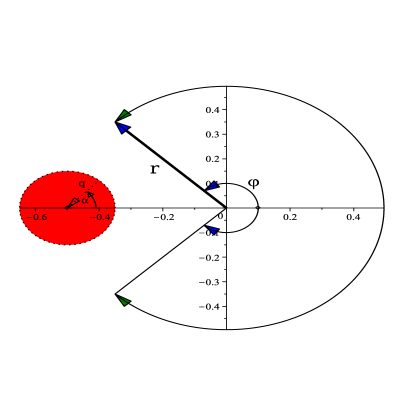
Now, we must ask what happens exactly at the pole, since this corresponds to integrals on the left-hand side of (4.3) and (4.4) of significant interest. Continuing from (6.3), let , and examine the joint limits and . This could be done by approaching the pole term by moving along the negative real axis starting from a point far from the singularity () to land on the pole, either from the right () or the left () by considering the limit as . See Figure 1. We find
| (6.4) |
This result shows that the real part (4.31) will vanish at the singularity, whereas the contribution to the imaginary part (4.32) will be indefinite. Alternatively, we may approach the limit point by choosing and consider the limit , effectively approaching the pole along a circle of radius , (again see Figure 1) in which case we find
| (6.5) |
indicating that the real part is indefinite and the imaginary part vanishes. So, we have an ambiguity. Notice that the left-hand sides of (4.31) and (4.32) are immune to the ordering of limits applied to the right-hand side – in fact, insofar as the left-hand sides are concerned, no limits are required because ; it is a case of simple substitution: and – leaving an entity with a clear symbolic meaning, but a foggy value.
Further thought indicates that this ambiguity duplicates what happens at any simple pole when it is analysed in the same manner. Consider the example
| (6.6) |
and let . In the vicinity of the pole we have
| (6.7) |
so if we approach the pole (i.e. ) along the line , the imaginary part of the function vanishes and the real part becomes indefinite. Approached along the line , the opposite occurs – the real part vanishes and the imaginary part becomes indefinite. Approached from any other direction, both real and imaginary parts become indefinite. This differs from an essential singularity where the limit of an approach from any direction will involve all possible values at the limit point; for similar examples, see [15, page 380] and [16, Section (1.4.2)].
The difference between (6.6) and (6.7) reflects the fact that the former involves a single complex variable ; the latter involves two independent real variables and , which as we shall see later, can be treated as both independent and complex. As noted by Vladimirov who discusses a similar example, [16, page 30], Hartog’s theorem: “If a function is holomorphic with respect to each variable individually, it is also holomorphic with respect to the entire set of variables” is not valid for functions of real variables.
6.1.1 Discussion
In short, we have arrived at a situation where a well-defined entity with a well-defined symbolic meaning has two, equally valid values. Which shall we choose? For the remainder of this Section, I will explore various possibilities that may resolve the ambiguity inherent in (6.4) and (6.5). The goal is to obtain a preferred and consistent choice, but that is not to say it is the only one.
At this point it is worth asking: can the singularity associated with this ambiguity be identified as a classified singularity, e.g. an essential singularity or a branch point? It is obvious that the singular point is not a “branch point” because it lies atop, but does not terminate a branch cut. However, the ambiguous limits displayed by (6.4) and (6.5) share some, but thus far, not all of the classification requirements of an essential singularity, one property of which requires that a function take on all values, except possibly one, as it approaches a limit point from all directions (Picard’s Second theorem - see definition (A.4)). As we have seen, the right-hand sides of (4.31) and (4.32) can be regularly expanded in a neighbourhood of the limit point, and the ratio (of independent variables) takes on many possible values as the limit point is approached along curves defined by those variables, but only three values at the limit point itself - see Figure 1.
For guidance, note that ambiguous limit points are known in the literature, but rarely discussed. In their tome dedicated to counterexamples, Gelbaum and Olmsted [17, Chapter 9, Ex. 7] present just such an example. In a footnote, Hardy [18, page 202] also gives an example but (perhaps wisely) defers further comment. Vladimirov makes reference to non-single-valued functions [16, Section I.8.5] and gives an example [16, Section 1.4.2] of a non-continuous function that is holomorphic for each variable individually in a neighbourhood of a limit point, but also eschews further discussion. Whittaker and Watson [19, page 100 ff] discuss the properties of an essential singularity in terms of a Laurent expansion, but never focus on how to deal with an ambiguous singularity at the limit point. Uniquely among authorities, Morse and Feshbach [15, page 380, ff] distinguish between the value of an essential singularity near the singularity and at the singularity and comment that “the behaviour of a function near an essential singularity is most complicated… their properties must therefore be carefully investigated in the neighbourhood of such points”, but offer no further guidance. All of the above limit their comments to an isolated singularity.
6.1.2 Analysis
The remainder of this Section is devoted to an examination of this phenomenon, as it applies to (4.31) annd (4.32), particularly to determine what happens when the limit point is approached from all directions - is Picard’s Second Theorem satisfied? What is the nature of the Laurent series?
To study the latter question, reconsider (6.5) expanded to more terms with less detail in order to survey the structure of the expansion. Applying the sequence of limits first, we find
| (6.8) |
where each of the coefficients is a function only of the parameters and contains no or dependence. The first terms in parentheses on the right-hand side indicates the existence of a regular part, the second term proves the existence of a single pole, and the other terms can be interpreted to be the first few terms of the Principle part of a Laurent series expansion about . Notice that the higher order terms of the expansion vanish if , leaving a single isolated simple pole at the limit point, but a Laurent expansion with a recognizable principle part nonetheless. Now, reconsidering (6.4), repeat the limiting exercise in the opposite order, that is apply the limit first, producing
| (6.9) |
where are expansion coefficients independent of both and . Here we again see a regular term as well as a sequence of terms that can be interpreted to be the Principle part of a Laurent expansion about . Significantly, the expansion factors in such a way that the terms of the Principle part series vanish if , leaving a simple pole and a regular term at the limit point. This is all consistent with the tentative interpretation that the limit point under consideration () is a non-isolated essential singularity with the unusual property that approached from certain directions, it reverts to a simple pole, a property antithetical to the properties of a run-of-the-mill essential singularity. It will shortly be shown how to utilize this property to overcome the ambiguity discussed above.
One way to deal with the ambiguity, employing the ordering limit used in (6.5) with , is to add the two results with multipliers and , and follow by setting , to eventually arrive at a more general, unambiguous identity
| (6.10) |
thereby removing an unremovable (essential) singularity – a textbook impossibility – suggesting that it is not an essential singularity. See Figures (2a) and (2b).
Another, more general way of treating this ambiguous limit suggests that we follow Vladimirov [16] by rewriting (4.31) and (4.32) in terms of two new variables defined by
| (6.11) |
where and arrives at the exceptional limit point. Effectively, we are evaluating (4.31) and (4.32) along a ray (defined by the angle ) of a circle of ever diminishing radius surrounding the exceptional complex point , corresponding to , in the previous co-ordinates. Again see Figure 1. After fairly lengthy calculations (Maple), we find the equivalents of (4.31) and (4.32) as follows
| (6.12) |
and
| (6.13) |
where
| (6.14) |
and
| (6.15) |
When , , creating a sign ambiguity in (6.12), but leaving (6.13) invariant. Both (6.12) and (6.13) can be verified numerically for and random values of . However, in addition to the ambiguity attached to discussed above, problems arise on the right-hand side when one attempts to determine the value of these identities at the limit point , which, of course, defines integrals of particular interest. Significantly, the numerator of the pole term on the right-hand side of both varies continuously and arbitrarily between depending on , so the right-hand side function itself takes on all values in the neighbourhood of the point as required by Picard’s Theorem; however its value at the limit point itself is again constrained to just three possibilities. In this respect, the limit point appears to satisfy the criterion that it is an essential singularity of the function on the right-hand side of both identities, and therefore creates a value ambiguity of the left-hand side by analytic continuation in the variable .
However, the “principle part” of the Laurent series of a function near an isolated essential singularity consists of an infinite series (in this case inverse powers of ) and as can be seen, here the principle part consists of a single pole term in the variable , not an infinite series of such terms. Furthermore, the pole term of an essential singularity cannot be removed; in the following, it will be shown how this can be done. And so, barring further insight, we must treat the singularity at the point as an unclassified singularity, possessing an aberrant pole, meaning that it vanishes when approached from some directions. We now proceed to show how it can be unambiguously removed.
6.2 Notation
In the following, I use the symbol to indicate that the value of the left-hand side of an identity possesses an (ambiguous) directional limit when the operation is applied to the right-hand side. This is in complete analogy to, and generalizes, the well-known symbol “” used to indicate a directed limit when an ambiguity exists (e.g. and ). Thus, with reference to the left-hand side (LHS) of (6.12) we could write
| (6.16) |
to mean
| (6.17) |
where the chosen value of takes precedence and the value is either finite determined by the leading order of q, or indefinite. Examples of the usual notation that deals with ambiguities (e.g. associated with an essential singularity) might include
| (6.18) |
or
| (6.19) |
if is constrained to , or, recognizing that the function requires a directional limit if , one could rewrite and write
| (6.20) |
to emphasize that a directional limit is required.
To investigate the properties of such identities, consider (6.13) when . On the left-hand side, it is sufficient to simply substitute and allow the (symbolic) notation to convey its meaning, but, significantly, not its value. On the right-hand side, which defines the value of the left-hand side by analytic continuation in the variable , as we have seen, there is an ambiguity in the ordering of limits. Notice that in all of the above, although the value of the left-hand side is assigned by an arbitrary ordering of limits of two independent variables, symbolically, there is no indication of this dependence. Insofar as the integrals are concerned, the variables and are “hidden variables” and the value of the integrals is determined by holomorphic continuation (regularization) in these variables.
Specifically, to evaluate the limit at a constant value of , one finds, from (6.13)
| (6.21) |
so that, if we have
| (6.22) |
Read from left-to-right, the value(s) of both sides depend on , one indirectly, the other directly, and are therefore indeterminate, although their meaning is quite clear. To reiterate, if one chooses to approach the limit point along one of the two rays defined by , then the value of the right-hand side is governed by the leading (finite) term in the expansion in the variable , otherwise it is indefinite. From (6.12) we similarly have
| (6.23) |
which, for the case yields
| (6.24) |
and an ambiguity arises depending on whether one chooses to approach the limit point along the ray(s) defined by or not.
In order to investigate consistency between identities obtained with and without ambiguity, it is convenient to introduce a means to tag cases where indeterminacy exists. Therefore, to label the default choice of an ambiguous operation, we shall use the symbol to tag an equality where an ambiguous directional limit exists, but a choice that will result in a finite limit has been made. Thus (6.24) with the choice would be written
| (6.25) |
Finally, and significantly, it is important to note that, in order to obtain a finite result in (6.13), we require the choice , i.e. , whereas to obtain a finite result in (6.12) we require the choice , i.e. , suggesting an inconsistency between the choice of limits for the real and imaginary parts of the two identities, unless the ambiguity is banished. It will now be shown how this can be achieved.
6.3 Removal of the ambiguity
6.3.1 Method A: Weighted Difference
To investigate one possible way to remove the ambiguity embedded in the above, obtain consistency and limit the analysis to that of finite quantities, apply the temporary condition that , then consider a weighted difference of (6.12) and (6.13), the former multiplied by , the latter by , yielding a single combined identity
| (6.26) |
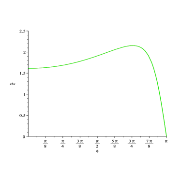
Since the divergent term no longer appears on its right-hand side, (6.26) is a simple, straightforward identity that can be tested numerically for reasonable values of and any value(s) of or one desires. However, as , the left-hand side becomes less and less amenable to numerical evaluation, and eventually confounds both Mathematica and Maple as , since it becomes heavily oscillatory and numerically intractable at the limit point . But, since the right-hand side of (6.26) is an entire function of for , and, by simply setting , the right-hand side yields the identity
| (6.27) |
it is clear that the singularity has been removed for the entire range of both variables and . Thus with no remaining singularities, the range and is a holomorphic domain of (6.26), so by the laws of analytic and holomorphic continuation, although was specifically excluded in it’s derivation, (6.26) is a perfectly well-defined identity for all including the points , the validity of which can be numerically verified when .
Therefore, when , the left-hand side of (6.26) remains represented by its right-hand side, which vanishes for all values of . By simple substitution in (6.26), special cases of interest with can be obtained by choosing special values of ; first set , to obtain
| (6.28) |
which, with yields
| (6.29) |
and second, let , to find
6.3.2 Method B: Choose
Continuing, consider a second possibility leading to an unequivocal result in a different way. In (6.12) and (6.13) set , and add, to eliminate the divergent term, yielding a simpler form of (6.26). Let , to obtain
| (6.35) |
Then repeat the same sequence with , to obtain
| (6.36) |
6.4 Eq. (6.26) and the exceptional case(s)
In the case , the exceptional point lies at , in which case (6.12) and (6.13) are virtually unchanged except that we employ in place of and we are dealing with , the alternating Zeta function, and indirectly Riemann’s function . In the following, having studied the intricacies of indeterminacy in the previous Section, only results will be given. The reader is encouraged to repeat the previous variations as an exercise.
To summarize, in the following, I use and throughout, with in the appropriate combination of identities equivalent to (6.26) with the substitutions given above, in which case indeterminism has been banished. Further, identities involving are usually transcribed in terms of (see (1.4)), since integrals written in the latter form are of greater general interest. The simplest identity found is
| (6.37) |
and
| (6.38) |
Remark: Prior to setting , the combined identities can easily be tested numerically for reasonable values of .
-
•
(6.39) and
(6.40) After adding and subtracting we get several identities relating the components of :
(6.41) and
(6.42) or
(6.43) -
•
From (6.38) we similarly find the general form
(6.44) so, for and respectively,
(6.45) and
(6.46) -
•
Adding and subtracting then gives
(6.47) and
(6.48) -
•
With reference to (6.32), (6.45) and (6.46) can be rewritten in the form
(6.49) and
where
(6.50) (6.51) and
(6.52) Remark: Excepting the latter three, it is not clear whether any of these integrals are numerically convergent, or obtain their value by analytic continuation (see Appendix A Lindelöf’s Hypothesis), since the asymptotic nature of remains unknown.
- •
-
•
As a numerical check, (6.53) predicts that
(6.56)
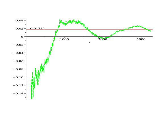
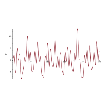
It is interesting to attempt to verify this identity numerically, notwithstanding the fact that it possesses a highly oscillatory integrand and may not converge, by partitioning the integral into small pieces, numerically integrating each small piece, and averaging the running partial sums. The result is shown in Figure 3. This is an example of either Cesàro summation or Cesàro regularization as the case may be [20, page 194], depending on whether the integral converges numerically or not. The outcome of the experiment shown in the Figure suggests that (6.56) is plausible and numerical convergence is a true possibility.
7 The exceptional cases Corollary 2.4,
For the remainder of this Section, we shall be considering the case and based on Corollary 2.4 i.e. (2.5).
7.1 The Real part
-
•
First, let so we are interested in the case that .
Consider the right-hand side of (5.2) labelled , where we again find that an ambiguity resides. This time, for full generality, let . The leading terms, as each of , independently is
(7.1) This demonstrates the indeterminism that we have come to expect, and, for the first time, also shows that the previous first level choice () has spared us from a higher order of indeterminism, even in the case that . To begin, let us now choose (i.e. ) followed by , (i.e. ), leaving a finite result, that being
(7.2) where the ordering of limits is to be read from right to left. From (B.4) and (7.2) with , we obtain the identity
(7.3) Combining (7.3) and (6.40) yields
(7.4) which, together with (5.24) reproduces (5.26), a non-exceptional result, demonstrating both consistency and indicating that the ordering in (7.2) was the preferred choice.
The case for general values of and general values of is fairly lengthy and is left as an exercise, but the result is again as predicted. In the case that we set and , (5.20) becomes
(7.5) Effectively, the right-hand side is of the form expected from (7.1), replete with a singularity that vanishes if . So, letting we find
(7.6) which reduces to (7.3) if . The identity (7.5) suggests that the singularity can be removed by combining two instances of that identity. For example set then and subtract with suitable multipliers. Alternatively use and and add; and is also a propitious choice. However, these variations lead to very long identities that show no promise of reducing to something simple, so are left as exercises for the reader.
It is also interesting to digress slightly by evaluating the same identity (B.4) in a different order. If , the equivalent identity becomes
(7.7) which can easily be numerically verified for small values of . However, in the limit , the right-hand side of (7.7) diverges as predicted by (7.1); specifically we find
(7.8) which should be compared to (7.3).
-
•
If , indeterminism again arises in (5.3).
Let to obtain
(7.9) an identity that is valid for all values of , particularly and does not appear to be indeterminate. However, considering the opposite directional limit, let , followed by and, let to obtain
(7.10) another indeterminism. Again, choosing (7.9) produces
(7.11) By choosing (7.9) it is possible to obtain an identity for the left-hand side at a constant value of , valid for all . Being rather lengthy, (but numerically verifiable for ), this identity is included as (B.7) in Appendix B. If , (7.11) reduces to (5.26). If , (7.11) becomes
(7.12) which can be combined with several of the results previously obtained to reproduce others already obtained. So, (7.12), is not an independent identity, although it was independently derived, and bears the tag of indeterminism because an alternative evaluation exists.
7.2 The imaginary part
-
•
In the case that and , let denote the right-hand side of (B.5).
If we first set , a choice emerges. For the case , with the limits to be read from right to left, and being as defined previously (see (7.1)), we have
(7.13) whereas
(7.14) a far more desirable, but not unique, outcome . From the preferential choice (7.14) we then have
(7.15) From previous results, it is possible to check this choice for consistency. Combine (7.15) with (5.34) to obtain
(7.16) Adding (7.16) and (5.33) yields
(7.17) and combining (7.17) with (5.32) reproduces (5.34), demonstrating consistency. It is also possible to show that the right-hand side of (7.15) is the only possible value that will reproduce this sequence of equalities, proving both that the above argument is not circular, and, at the same time, that (7.15) is not independent of the other identities, although it was derived independently. Finally, on the same ordering basis as (7.14), for and , we find
(7.18) If , (7.18) becomes
(7.19) -
•
In the case , define to represent the right-hand side of (B.2). With and we have two possible limits, similar to those given in(7.14):
(7.20) whereas an alternative is
(7.21) Notice that the non-singular part of (7.20) differs from the leading terms of (7.21). In keeping with accumulating experience, we shall choose to employ (7.21) rather than attempting to eliminate the singular term in (7.20), in which case, (B.2) becomes
(7.22) reducing to (5.34) when , suggesting that (7.21) was a preferred choice. If , we find
8 A Principal Value analogue
Although many of the identities quoted so far started as functions of the single complex variable and morphed into meromorphic functions of the real variables and considered independently, the analytic structure is shared between both sides. So, by the “Edge of the Wedge” theorem [16, pages 251 ff. ], which states that, with sufficient conditions on analyticity, analytic continuation is valid along a line corresponding to the real part of one of several complex variables, this is sufficient to allow both and to be treated as independent real variables as has been done throughout. Now consider an extension such that becomes complex.
If one writes and simultaneously , the variable is unchanged. However, now let , with no change in , being equivalent to adding an imaginary () axis perpendicular to the plane of Figure 1. Since each of the original identities develops a new real and imaginary part, this generates a new set of identities, the left-hand sides of which are easily written, the right-hand sides, lengthy and not so easily reported (this is left as an exercise for the reader using computer algebra). With , the four integrals that arise are the following:
| (8.1) | |||
| (8.2) | |||
| (8.3) | |||
| (8.4) |
In special cases, the right-hand sides simplify considerably, so, for the record the following presents the corresponding non-zero identities when :
| (8.5) | |||
| (8.6) |
For , there are no singularities in these cases, all of which can also be verified numerically.
8.1 The case
Now consider the case . If – this defines exceptional cases where one indexed term in the denominator vanishes – we find the non-zero identities
| (8.7) | |||
| (8.8) |
From these exceptional cases, arises another possibility to deal with the ambiguous singularity discussed throughout. To demonstrate the possibilities, here I consider only the case in detail. In (8.2) set followed by ; then evaluate the limit , to find, in either case
| (8.9) |
This result is valid for all , and diverges with a simple pole if , where it reduces to the results obtained previously, but becomes considerably more complicated if where is a positive integer. Alternatively, repeat the exercise but in the opposite order. First, in (8.2), let followed by , and in the limit , we find
| (8.10) |
demonstrating the indeterminism that has pervaded this work. Now, considering that the singular term in (8.10) changes sign depending on which of the two polarities of one chooses, it becomes possible to remove the singularity by adding the two versions of (8.10) corresponding to and signs. This is analogous to a Principal Value regularization, where a contour along a real axis is deformed above and below the axis into the imaginary part of the complex plane to avoid a singularity . After performing the addition, and following considerable simplification (Maple) we find
| (8.11) |
In this variation, no limits were applied, so the result is deterministically exact, although numerically unverifiable. Note that the left-hand sides of (8.9) and (8.11) differ, but they share pole terms at that differ in magnitude by a factor of two. Thus subtracting (8.9) and (8.11) with a suitable multiplier, yields a new result, equivalent to one of the identities obtained previously using the same variables. In fact for the case we find,
| (8.12) |
In Appendix B, the general case () is listed (see (B.3)). Because the singularity at has now been removed, by taking the limit on the right-hand side of (8.12) and expanding the left-hand side about , we recover (4.44); also, since both sides can be expressed in even powers of , the next moment corresponding to the coefficients of gives the identity
| (8.13) |
in agreement with the higher order differentiation of (4.44).
9 Summary
In a fairly lengthy exposition, I have evaluated a number of improper integrals containing Riemann’s zeta and related functions that are likely new, and identified a pathology which, in some respects, emulates an essential singularity but is not. It arises because the analysis is based on the use of two real variables, which, as noted, do not obey the usual rules attached to complex variables. However, although the pathology gives rise to the unusual property of indeterminism, notably the necessity of distinguishing a directional from a directed limit, similar multi-valued entities are not unknown, but, to the best of my knowledge they do not arise in the evaluation of an integral. In fact, Whitehead and Russel [21, page 17, also page 41, Chapter II], write (in paraphrase):“… the meaning of (definite integral) involves the supposition that such a field is determinate”.
In order to arrive at a useful calculus embodying the directional limit, several different methods were explored, each of which succeeded in arriving at a meaningful and self-consistent result. As noted, and to reiterate, in some cases it was possible to compare two identities, one of which was calculated according to the accepted methods of analysis, the other by means of the method in which the pathology was circumvented. In all cases the comparison yielded consistency. In one instance, a numerical experiment was attempted in order to check the plausibility of a predicted result. In order to focus on the identified pathology, many threads were left hanging. A few possibilities that seem to merit future study include the application of the results reported here to:
-
•
Indeterminism: By removing the pathology, a self-consistent calculus arose involving finite quantities, but the possibility remains that a different choice could have been made resulting in singular quantities. Is it possible that this second choice will yield a self-consistent calculus and, if so, what does it mean? Notice the difference between the regular parts of (7.20) and (7.21).
-
•
Off the Critical Line: Throughout, for brevity, most examples were chosen to lie on the critical line , although the methodology allows for a more general choice. In a few places - see (7.1) and (7.5) - there were suggestions that choosing to evaluate an integral along the critical line creates a new level of indeterminism that may distinguish the critical line from elsewhere in the critical strip. Is this significant?
-
•
Universality: The concept of Universality states that approaches arbitrarily close to any function inside a circle of radius centred on the line - see [3, Chapter XI]. The integrand of (3.1) consists of positive terms only, and therefore that identity places a numerical limit on the value of integrated over the same range as Universality is said to apply. Are these two concepts consistent? How? Does this lead to an inequality for the integrated value of the absolute value of the set of all possible functions over the strip ?
-
•
Integral transforms: Many of the results quoted here effectively define the coefficients of the cosine and sine transforms of the function - see (5.36) for example. Is it possible to express as a Fourier or Laplace transform in closed form - see [2, Section 8.2], other than via (2.3) and known transformations among Mellin and other transforms - see [20]?
-
•
Moments: Several samples were given of the higher moments for the integrals being studied - see (4.21) for example. Is there a general form? Does it lead to new identities?
-
•
Mean Value Formulae: In [22, Section 11.4], Ivić studies the asymptotic limit of the integral
(9.1) Can (9.1) be related to integrals studied here, perhaps by extending ?
-
•
By Parts: Does integration by parts applied to any of the identities presented lead to new identities?
-
•
Extension: There is no requirement that the variable in Section 3 be real. What happens if it becomes complex?
10 Acknowledgements
11 Declarations
: Funding: All expenses related to this work have been borne by the author.
: Conflicts of interest None.
: Availability of data and material All relevant material is contained herein.
: Code availability N/A
: Authors’ contributions This is the work of the sole author.
: Ethics approval N/A
: Consent to participate N/A
: Consent for publication N/A
References
- [1] R.B. Paris and D. Kaminski. Asymptotics and Mellin-Barnes Integrals, volume 85 of Encyclopedia of Mathematics and its Applications. Cambridge University Press, Cambridge, U.K., 2001.
- [2] Aleksandar Ivić. The theory of Hardy’s Z-Function, volume 196 of Cambridge tracts in Mathematics. Cambridge University Press, New York, 2013.
- [3] E.C. Titchmarsh and D.R Heath-Brown. The Theory of the Riemann Zeta-Function. Oxford Science Publications, Oxford, Second edition, 1986.
- [4] Niels Nielsen. Handbuch der Theorie der Gammafunktion. Druck und Verlag von B.G. Teubner, Leipzig, 1906. reprinted from the original by Wentworth Press.
- [5] Daeyeoul Kim Su Hu and Min-Soo Kim. Special values and integral representations for the Hurwitz-type Euler Zeta functions. J. Korean Math. Soc.,, 55(1):185–210, 2018. https://doi.org/10.4134/JKMS.j170110.
- [6] Olivier Espinosa and Victor H. Moll. On some integrals involving the Hurwitz Zeta function: Part 1. The Ramanujan Journal, 6:159–188, 2002. also available from https://doi.org/10.1023/A:1015706300169 or https://arxiv.org/0012078v1.
- [7] M. A. Shpot and R. B. Paris. Integrals of products of Hurwitz zeta functions via Feynman parametrization and two double sums of Riemann zeta functions. May 2020. available from https://arxiv.org/pdf/1609.05658.
- [8] F. W. J. Olver, D. W. Lozier, R. F. Boisvert, and C. W. Clark, editors. NIST Handbook of Mathematical Functions. Cambridge University Press, New York, NY, 2010. Print companion to [23].
- [9] A.P. Prudnikov, Yu. A. Brychkov, and O.I. Marichev. Integrals and Series: More Special functions, volume 3. Gordon and Breach Science Publishers, New York, 1986.
- [10] Wolfram Research, Champaign, Illinois. Mathematica, version 12, 2020.
- [11] Maplesoft, a division of Waterloo Maple Inc., version 2021. Maple.
- [12] Donal F. Connon. On an integral involving the digamma function, 2012. available from https://arxiv.org/abs/1212.1432.
- [13] Marc-Antoine Coppo and Bernard Candelpergher. A note on some formulae related to Euler sums. hal-03170892v4, 2021. available from https://hal.univ-cotedazur.fr/hal-03170892v4.
- [14] I.S. Gradshteyn and I.M. Ryzhik. Tables of Integrals, Series and Products, corrected and enlarged Edition. Academic Press, 1980.
- [15] Morse P.M. and Feshbach H. Methods of Theoretical Physics, Part 1. McGraw-Hill Book Company Inc., Toronto, 1953.
- [16] Vasiliy Sergeyevich Vladimirov. Methods of the Theory of Functions of Many Complex Variables. Dover Publications Inc, Mineola, New York, 2007. Translated from the Russian by MIT Press, 1966.
- [17] Gelbaum Bernard R. and Olmsted John M.H. Counterexamples in Analysis. Holden-Day Inc, San Francisco, 1964.
- [18] G.H. Hardy. Pure Mathematics. Cambridge at the University Press, 1945.
- [19] Whittaker E.T. and Watson G.N. A Course of Modern Analysis. Cambridge University Press, 1950.
- [20] Widder D.V. An Introduction to Transform Theory. Academic press, New York, 1971.
- [21] Whitehead A.N. and Russell B. Principia Mathematica, volume I. Cambridge University press, Cambridge, U.K., 1910.
- [22] Borwein P., Choi S., Rooney B., and Weirathmueller A. The Riemann Hypothesis : a resource for the afficionado and virtuoso alike. CMS books in mathematics. Springer, New York, 2008.
- [23] NIST Digital Library of Mathematical Functions. http://dlmf.nist.gov/, Release 1.0.9 of 2014-08-29.
- [24] E.C. Titchmarsh. The Theory of Functions, Second Edition. Oxford University Press, 1939, reprinted and corrected 1949.
- [25] E.W. Weisstein. Analytic continuation. mathworld – a wolfram web resource., 1999-2001. Retrieved from https://mathworld.wolfram.com/AnalyticContinuation.html.
- [26] Euler L. Institutiones Calculi Integralia, volume IV. 1794.
Appendix A Definitions and Identities
A.1 Definitions
In the entirety of this work, and are always non-negative integers except where noted; all other symbols are complex, except where noted. (i.e. polygamma) is the derivative of the digamma function, except for the first derivative written as . is the Euler-Mascheroni constant, is the first Stieltjes constant in the expansion of . Throughout, the symbol may be referenced by its real and/or imaginary components, that is where . Other symbols are defined either as they appear, or in this Appendix. Any sum whose lower limit exceeds its upper limit is zero. The real and imaginary components of a complex function are denoted by subscripts and respectively. Complicated and lengthy identities are frequently quoted; these were obtained by either of the computer codes Mathematica [10] or Maple [11], which are cited by name at the corresponding points in the text. By way of review:
Definition A.1.
Holomorphic function: “A function is said to be holomorphic at a point if, in some neighbourhood of , it is the sum of an absolutely convergent power series . [16, Section I.4.1] - Weierstrass’ defintion”.
Definition A.2.
Domain of holomorphy: “To every holomorphic function there corresponds a unique domain of holomorphy, namely, the domain of existence of the function” [16, Section I.8.6]”.
Definition A.3.
Singular points: “The boundary points of a domain of holomorphy of a function are called the singular points of that function” [16, Section I.8.7]”.
Definition A.4.
Essential Singularity: “In the neighbourhood of an isolated essential singularity, a one-valued function takes every value, with one possible exception, an infinity of times” [24, Picard’s Second Theorem, page 283].
Definition A.5.
Lindelöf’s Hypothesis “The Lindelöf Hypothesis is that for every positive and every ” [3, Chapter XIII].
Definition A.6.
Analytic Continuation: “Let and be analytic functions on domains and , respectively, and suppose that the intersection is not empty and that on . Then is called an analytic continuation of to , and vice versa. Moreover, if it exists, the analytic continuation of to is unique.” [25]
A.2 Identities and Lemmas
-
•
By splitting the sum (1.2) into its even and odd parts it is easily shown that
(A.1) - •
-
•
From [19, Section 13.21]
(A.3) -
•
From [8, Eqs. (5.4.3), (5.4.4) and (5.7.6) respectively] we have
(A.4) (A.5) and
(A.6) -
•
Differentiating (2.1) with respect to yields
(A.7) -
•
From Maple [11]
(A.8) -
•
Based on [8, Eq. (5.7.6)] we separate the real and imaginary parts of a special case of the digamma function:
(A.9) and
(A.10)
Appendix B Long Equations
Here we collect many of the most general results used throughout to obtain special case identities.
B.1 Constants
| H | 0.73128770329627095609488699144402008790399467173125… |
|---|---|
| B | 0.011631879936622239647933640848662374256023406252918… |
| 0.0080562886088479438618780062072017192398728472183716… | |
| 0.070086041002631260196371300230060136931855307780993… | |
| -0.034562106682472096758925963508715396071235328556772… |