Symbiotic solitons in a quasi-one- and quasi-two-dimensional spin-1 condensates

Abstract

We study the formation of spin-1 symbiotic spinor solitons in a quasi-one- (quasi-1D) and quasi-two-dimensional (quasi-2D) hyper-fine spin $F=1$ ferromagnetic Bose-Einstein condensate (BEC). The symbiotic solitons necessarily have a repulsive intraspecies interaction and are bound due to an attractive interspecies interaction. Due to a collapse instability in higher dimensions, an additional spin-orbit coupling is necessary to stabilize a quasi-2D symbiotic spinor soliton. Although a quasi-1D symbiotic soliton has a simple Gaussian-type density distribution, novel spatial periodic structure in density is found in quasi-2D symbiotic SO-coupled spinor solitons. For a weak SO coupling, the quasi-2D solitons are of the $(-1,0,+1)$ or $(+1,0,-1)$ type with intrinsic vorticity and multi-ring structure, for Rashba or Dresselhaus SO coupling, respectively, where the numbers in the parentheses are angular momenta projections in spin components $F_{z}=+1,0,-1$, respectively. For a strong SO coupling, stripe and superlattice solitons, respectively, with a stripe and square-lattice modulation in density, are found in addition to the multi-ring solitons. The stationary states were obtained by imaginary-time propagation of a mean-field model; dynamical stability of the solitons was established by real-time propagation over a long period of time. The possibility of the creation of such a soliton by removing the trap of a confined spin-1 BEC in a laboratory is also demonstrated.

I Introduction

A bright soliton Kivshar or a soliton is a self-bound solitary wave that can move at a constant velocity maintaining its shape due to a cancellation of non-linear attraction and linear repulsion. Bright solitons have been created and studied in a ⁷Li li and ⁸⁵Rb rb Bose-Einstein condensate (BEC) by controlling the non-linear attraction near a Feshbach resonance Inouye , so that the atomic scattering length is changed to a desired negative value. A vector soliton is a solitary wave with multiple components that maintains its shape during propagation. An ordinary soliton has effectively only one (scalar) component or species, while vector solitons have more than one distinct species. Most of the vector solitons studied so far are self attractive, so that, due to an intraspecies attraction, vector solitons can be realized independent of the nature of the interspecies interaction: attractive or repulsive. However, it is also possible to create a self-repulsive binary (two-component) vector soliton where the intraspecies interaction is repulsive Perez-Garcia . In that case a vector soliton is formed due to an interspecies attraction where the presence of different species is fundamental for the formation of the vector soliton. Such a self-repulsive vector soliton is usually called a symbiotic soliton.

Most studies of a symbiotic soliton involve only two distinct species, because it is difficult to realize a three-component hetero-nuclear BEC experimentally. After the experimental observation of a hyper-fine spin $F=1$ exp spinor BEC of ²³Na atoms, self-attractive pseudo spin-1/2 spinor solitons have been extensively studied in spinor BECs Ieda . The interspecies interaction in a spin-1 spinor BEC is very different from that in a three-component hetero-nuclear BEC and it is not a priori clear that a symbiotic soliton can be formed in a spin-1 spinor BEC. In this paper we demonstrate that a dynamically-stable symbiotic soliton can indeed be formed in a quasi-one-dimensional (quasi-1D) spin-1 spinor BEC and study its statics and dynamics. The viability of the formation of a quasi-1D spin-1 symbiotic soliton by removing the trap of a confined spin-1 BEC in a laboratory is also demonstrated.

A quasi-two-dimensional (quasi-2D) or a three-dimensional soliton cannot be stabilized in a BEC due to a collapse instability Kivshar ; coll . However, it has been demonstrated that a quasi-2D soliton can be formed in a pseudo spin-1/2 spinor BEC in the presence of a spin-orbit (SO) coupling malo . There have been studies of solitons in a quasi-1D pseudo spin-1/2 SO-coupled BEC rela , in a quasi-1D spin-1 SO-coupled BEC sol1d and in a quasi-2D spin-1 SO-coupled BEC sol2d . Although, there could not be a natural SO coupling in an atomic spinor BEC, an artificial synthetic SO coupling can be realized in such a BEC using tuned Raman lasers coupling the different spin states stringari ; rev . Two such possible SO couplings are due to Rashba Rashba and Dresselhaus Dresselhaus and other types of SO coupling are also possible. An equal mixture of Rashba and Dresselhaus SO couplings has been realized experimentally in a pseudo spin-1/2 ⁸⁷Rb 11 and ²³Na 12 BEC of $F_{z}=0,-1$ spin states. Later, an SO-coupled spin-1 ⁸⁷Rb BEC of $F_{z}=\pm 1,0$ states was observed and investigated 13 following a suggestion SOspin1 .

In view of these, we explore the possibility of the formation of a quasi-2D symbiotic SO-coupled spin-1 spinor soliton and demonstrate that such a soliton can indeed be created with different spatial periodic patterns in density. For a weak SO coupling, $(\mp 1,0,\pm 1)$-type kita multi-ring solitons are found for a Rashba or a Dresselhaus SO coupling, where the upper (lower) sign corresponds to Rashba (Dresselhaus) SO coupling. These solitons have angular momenta projections $(\mp 1,0,\pm 1)$ at the center of $F_{z}=+1,0,-1$ components, respectively, where the positive (negative) sign inside the parenthesis denotes a vortex (antivortex). For a larger SO coupling, two different types of quasi-degenerate solitons are found. In the first type, the multi-ring solitons evolve into a new type of metastable solitons with broken angular symmetry. In the second type, the solitons develop a spatially-periodic pattern in density in the form of a stripe or a square-lattice modulation. These solitons usually have very large spatial extention. In all cases the soliton densities and energies are the same for both Rashba and Dresselhaus SO couplings although the two wave functions are different. We demonstrate the possibility of the formation of a quasi-2D symbiotic SO-coupled spin-1 spinor soliton in a laboratory by suddenly removing the trap of a trapped BEC.

A quasi-2D symbiotic SO-coupled spin-1 spinor soliton, with a periodic stripe or a square-lattice modulation in density, is quite similar to a supersolid sprsld . A supersolid is a quantum state, where matter forms a periodic rigid structure, breaking continuous translational symmetry, as in a crystalline solid, and enjoying friction-less flow, as in a superfluid, breaking Gauge symmetry. Supersolidity has been suggested 26 and observed 27 in a dipolar BEC. In a pseudo spin-1/2 SO-coupled BEC of ²³Na atoms, supersolidity was realized experimentally 28 in the form of a quasi-1D stripe pattern in density. In a quasi-2D symbiotic SO-coupled spin-1 spinor stripe soliton, only the component densities acquire a 2D stripe modulation, whereas in a superlattice soliton both component and total densities develop a 2D square-lattice modulation. The present quasi-2D symbiotic spin-1 soliton with a 2D square-lattice pattern in both component and total densities, sharing properties with a conventional supersolid, will be termed a symbiotic superlattice soliton following a previous suggestion adhik ; 29 . The quasi-2D symbiotic spin-1 soliton with a stripe pattern only in component densities will be called a stripe soliton, although such a state has often been called a super-stripe state in the literature. The superlattice spin-1 spinor soliton is a quasi-2D generalization adhik of the quasi-1D super-stripe pseudo spin-1/2 trapped BEC 29 with a stripe pattern in total density. The multi-ring solitons only exhibit a quasi-periodic structure in the component densities without a prominent periodic structure in total density.

A spin-$1$ spinor BEC is controlled by two interaction strengths, e.g., $c_{0}\propto(a_{0}+2a_{2})/3$ and $c_{2}\propto(a_{2}-a_{0})/3$, with $a_{0}$ and $a_{2}$ the scattering lengths in total spin $F=0$ and 2 channels, respectively Ohmi . All spin-1 spinor BECs can be classified into two distinct types Ohmi ; stringari : ferromagnetic ($c_{2}<0$) and anti-ferromagnetic ($c_{2}>0$). In this paper, we study three-component spin-1 symbiotic vector solitons in quasi-1D and quasi-2D traps using a numerical solution of the respective mean-field coupled Gross-Pitaevskii (GP) equation gp by imaginary-time simulation. These symbiotic solitons should have intraspecies repulsion, requiring $c_{0}>0$. In addition, if we take identical densities in spin components $F_{z}=\pm 1$ and $c_{2}<0$ (ferromagnetic), it is possible to have a quasi-2D symbiotic spin-1 spinor soliton of the ferromagnetic type bound by interspecies attraction, although some interspecies interactions are repulsive. For a quasi-1D symbiotic spin-1 spinor soliton, we present an approximate analytic solution in good agreement with the numerical result. We study the dynamics of the symbiotic soliton numerically by real-time simulation and establish its dynamical stability.

In Sec. II.1 and II.2, we describe the mean-field model GP equation for a quasi-1D symbiotic tertiary (three-component) BEC soliton and a quasi-1D symbiotic spin-1 spinor BEC soliton, respectively. We also provide an analytic solution of the model for these cases. In Sec. II.3, we present the mean-field GP equation for a quasi-2D symbiotic SO-coupled spinor soliton. In Sec. III.1.1, numerical result for energy and density of the stationary quasi-1D symbiotic spin-1 spinor BEC soliton is compared with the analytic approximation. In Sec. III.1.2, numerical result for energy and density of a quasi-2D symbiotic SO-coupled spin-1 spinor multi-ring, stripe and superlattice BEC soliton is presented. In Secs. III.2.1 and III.2.2 dynamical stability of a quasi-1D symbiotic spin-1 spinor BEC soliton and a quasi-2D symbiotic SO-coupled spin-1 spinor BEC soliton is established numerically. In Sec. III.2.1, we also demonstrate that a symbiotic spin-1 spinor BEC soliton can be created in a laboratory by removing the trap of a confined BEC with the same parameters. In Sec. IV a summary of our findings is presented.

II Theoretical Formulation

II.1 Quasi-1D symbiotic tertiary soliton

In a multi-component BEC, most studies on solitons are in self-attractive systems where the intraspecies nonlinearities are attractive. Here we consider the formation of a symbiotic tertiary soliton in a self-repulsive three-component BEC, where the intraspecies nonlinearities are repulsive; the soliton is bound by the attractive interspecies nonlinearities. Similar binding is possible in a symbiotic binary soliton Perez-Garcia . A tertiary BEC is described by the following GP equation, for the wave-function components $\psi_{i}(x,t),$ $i=1,2,3$, in dimensionless units:

$$\text{i}{\partial_{t}\psi_{i}(x,t)}=\big{[}-{\textstyle\frac{1}{2}}{\partial_{x}^{2}}+{g}_{0}|\psi_{i}|^{2}+g^{\prime}{\textstyle\sum}_{\bar{i}\neq i}|\psi_{\bar{i}}|^{2}\big{]}\psi_{i}(x,t),$$ (1)

where $\text{i}=\sqrt{-1}$, the partial space and time derivatives are denoted $\partial_{x}\equiv\partial/\partial x$ and $\partial_{t}\equiv\partial/\partial t$ and $g_{0}$ $(>0)$ and $g^{\prime}$ $(<0)$ are repulsive intraspecies and attractive interspecies nonlinearities, respectively. For simplicity we have taken the intraspecies and interspecies nonlinearities to be equal for different components and this simplifies the analytic treatment but otherwise has no effect on the formation of a symbiotic tertiary soliton. The time-independent stationary solution $\psi_{i}(x)$ satisfies $\psi_{i}(x,t)\equiv\psi_{i}(x)\exp(-\text{i}\mu t)$ with

$$\mu\psi_{i}(x)=\big{[}\textstyle-\frac{1}{2}{d_{x}^{2}}+{g}_{0}|\psi_{i}|^{2}+g^{\prime}{\sum}_{\bar{i}\neq{i}}|\psi_{\bar{i}}|^{2}\big{]}\psi_{i}(x),$$ (2)

where $d_{x}=d/dx$ and $\mu$ is the chemical potential. As in this case the three components are equivalent, the spatial dependence of the three components will be the same:

$$\psi_{i}(x)\equiv\textstyle\frac{1}{\sqrt{3}}\Phi(x),\quad i=1,2,3;$$ (3)

so that $|\Phi(x)|^{2}=\sum_{i}|\psi_{i}(x)|^{2}$, where $\Phi(x)$ satisfies the following GP equation

$${\mu\Phi(x)} =\big{[}-\textstyle\frac{1}{2}{d_{x}^{2}}+{g}|\Phi|^{2}\big{]}\Phi(x).$$ (4)

The consistency between Eqs. (2)-(4) requires $g=(g_{0}+2g^{\prime})/3$. As the intraspecies nonlinearity $g_{0}$ is repulsive (positive), for a solitonic solution the interspecies nonlinearity $g^{\prime}$ must be attractive (negative) and also $2|g^{\prime}|>g_{0}$ so that the effective nonlinearity $g$ is attractive (negative). The following secant hyperbolic function is the normalized analytic solution to Eq. (4) malomed

$$\Phi(x)=\frac{\sqrt{|g|}}{2}\mbox{sech}\left(\frac{|g|x}{2}\right).$$ (5)

The energy functional of this solution yields the following analytic estimate of energy

$$E_{a}=\textstyle\frac{1}{2}{\textstyle\int_{-\infty}^{\infty}}dx\left[|d_{x}\Phi(x)|^{2}+g|\Phi(x)|^{4}\right]=-\frac{g^{2}}{24}.$$ (6)

II.2 Quasi-1D symbiotic spin-1 soliton

II.2.1 Mean-field equation

We consider a quasi-1D spin-1 spinor BEC along the $x$ axis realized by strong harmonic traps in the $y-z$ plane, so that the system is frozen in the Gaussian ground state in these directions Salasnich . A quasi-1D spin-1 BEC of $N$ atoms can be described by the following set of three-coupled mean-field partial differential GP equations for the wave-function components $\psi_{i}(x,t),$ $i=+1,0,-1$ in dimensionless units Ohmi ; sol1d

$$\text{i}{\partial_{t}\psi_{\pm 1}} =\big{[}-{\textstyle\frac{1}{2}}\partial_{x}^{2}+{c}_{0}{n}\big{]}\psi_{\pm 1}$$

$$+c_{2}[{n}_{\pm 1}+{n}_{0}-{n}_{\mp 1}]\psi_{\pm 1}+c_{2}\psi_{0}^{2}\psi_{\mp 1}^{*},$$ (7)

$$\text{i}{\partial_{t}\psi_{0}} =\big{[}-\textstyle\frac{1}{2}\partial_{x}^{2}+{c}_{0}{n}\big{]}\psi_{0}$$

$$+c_{2}[{n}_{+1}+{n}_{-1}]\psi_{0}+2{c}_{2}\psi_{0}^{*}\psi_{+1}\psi_{-1},$$ (8)

where the interaction strengths are abc2

$${c}_{0}=\frac{2N(a_{0}+2a_{2})l_{0}}{3l^{2}_{yz}},\quad{c}_{2}=\frac{2N(a_{2}-a_{0})l_{0}}{3l^{2}_{yz}},$$ (9)

and component density ${n}_{i}(x)=|\psi_{i}(x)|^{2}$ with $i=+1,0,-1$ corresponding to the three spin components $F_{z}=+1,0,-1$, total density ${n}(x)=\sum n_{i}(x)$; $l_{yz}$ is the harmonic oscillator length in the transverse $yz$ plane and $l_{0}$ is an arbitrary scaling length in the $x$ direction. The length is measured in units of $l_{0}$ and densities in units of $l_{0}^{-1}$. A spin-1 spinor BEC is classified into two magnetic phases: ferromagnetic ($c_{2}<0$) and antiferromagnetic ($c_{2}>0$). The total density is normalized to unity, i.e., $\int{n}({x})d{x}=1.$ The conserved magnetization is $m=\int dx[n_{+1}(x)-n_{-1}(x)].$ The time-independent stationary state $\psi_{i}(x)$ satisfies $\psi_{i}(x,t)\equiv\psi_{i}(x)\exp(-\text{i}\mu_{i}t)$, with

$$\textstyle\mu_{\pm 1}\psi_{\pm 1} =\big{[}-\textstyle\frac{1}{2}d_{x}^{2}+{c}_{0}{n}\big{]}\psi_{\pm 1}$$

$$+c_{2}[{n}_{\pm 1}+{n}_{0}-{n}_{\mp 1}]\psi_{\pm 1}+c_{2}\psi_{0}^{2}\psi_{\mp 1}^{*},$$ (10)

$$\mu_{0}\psi_{0} =\big{[}-\textstyle\frac{1}{2}d_{x}^{2}+{c}_{0}{n}\big{]}\psi_{0}$$

$$+c_{2}[{n}_{+1}+{n}_{-1}]\psi_{0}+2{c}_{2}\psi_{0}^{*}\psi_{+1}\psi_{-1},$$ (11)

where $\mu_{i}$ is the chemical potential. The energy functional for a stationary state described by the mean-field GP equations (10) and (11) is Ohmi

$$E =\textstyle\frac{1}{2}\int_{-\infty}^{\infty}dx\big{[}\sum_{j}\left|{d_{x}\psi_{j}}\right|^{2}+c_{0}n^{2}+c_{2}\big{\{}n_{+1}^{2}+n_{-1}^{2}$$

$$+2\left(n_{+1}+n_{-1}\right)n_{0}-2n_{+1}n_{-1}$$

$$+2\left(\psi_{-1}^{*}\psi_{0}^{2}\psi_{+1}^{*}\right.\left.+\psi_{-1}\psi_{0}^{*2}\psi_{+1}\right)\big{\}}\big{]}.$$ (12)

II.2.2 Analytic Consideration

Numerical calculation for the ground-state densities of a ferromagnetic BEC $(c_{2}<0)$ has revealed that the component densities are essentially multiples of each other according to abc2

$$\psi_{i}(x)=\alpha_{i}\Phi(x),\quad i=\pm 1,0,$$ (13)

where $\alpha_{j}$ is in general complex. Equation (13), when substituted in Eqs. (10)-(11), leads to three equations for the same function $\Phi$. A consistency between these three equations require that $\Phi(x)$ satisfies Eq. (4) with the analytic solution (5) with $g=c_{0}+c_{2}$ and abc2

$$\psi\equiv\left(\begin{array}[]{c}\psi_{+1}\\ \psi_{0}\\ \psi_{-1}\end{array}\right)=\frac{1}{2}\left(\begin{array}[]{c}(1+m)\Phi(x)\\ \sqrt{2(1-m^{2})}\Phi(x)\\ (1-m)\Phi(x)\end{array}\right).$$ (14)

For a self-repulsive quasi-1D symbiotic spin-1 BEC soliton, $c_{0}$ must be positive (repulsive) and $c_{2}$ has to be negative (attractive), in addition to the condition $g\equiv c_{0}+c_{2}<0$ necessary for the system to have overall attraction. But, for a negative $c_{2}$, in Eq. (7) there is the self-attractive term $c_{2}n_{\pm 1}\psi_{\pm 1}$ in components $i=\pm 1$. However, if we are limited to the solution with the property $n_{+1}=n_{-1}$, leading to zero magnetization ($m=0$), Eq. (7) becomes

$$\textstyle\text{i}{\partial_{t}\psi_{\pm 1}}=\big{[}-\frac{1}{2}{\partial_{x}^{2}}+{c}_{0}{n}\big{]}\psi_{\pm 1}+c_{2}{n}_{0}\psi_{\pm 1}+c_{2}\psi_{0}^{2}\psi_{\mp 1}^{*}.$$ (15)

Hence, all solutions of Eqs. (8) and (15) for $c_{0}>0$ and $c_{2}<0$ satisfying $n_{+1}(x)=n_{-1}(x)$ represent quasi-1D symbiotic spin-1 spinor solitons, where a positive $c_{0}$ and negative $c_{2}$ correspond to intraspecies repulsion and interspecies attraction. Some interspecies interactions (proportional to $c_{0}$) in this model are repulsive. Nevertheless, all interspecies interactions (proportional to $c_{2}$) are attractive and the symbiotic vector soliton is formed due to these interspecies attractions. As $\Phi(x)$ satisfies Eq. (4) with $g=c_{0}+c_{2}$, analytic approximation (14) for $n_{+1}(x)=n_{-1}(x)$ and $m=0$, appropriate for a quasi-1D symbiotic spin-1 spinor soliton, becomes

$$\left(\begin{array}[]{c}\psi_{+1}(x)\\ \psi_{0}(x)\\ \psi_{-1}(x)\end{array}\right)=\frac{\sqrt{|c_{0}+c_{2}|}}{4}\mbox{sech}\left[\frac{|c_{0}+c_{2}|x}{2}\right]\left(\begin{array}[]{c}1\\ \sqrt{2}\\ 1\end{array}\right),$$ (22)

with the analytic energy

$$E_{a}=-\textstyle\frac{1}{24}(c_{0}+c_{2})^{2}.$$ (23)

II.3 Quasi-2D symbiotic SO-coupled spin-1 soliton

II.3.1 Mean-Field Equation

Because of a collapse instability, a quasi-2D soliton cannot be stabilized coll . However, a stabilized quasi-2D symbiotic spinor soliton is possible in the presence of an SO coupling. We consider a quasi-2D SO-coupled spin-1 spinor BEC in the $x-y$ plane realized by a strong harmonic trap along the $z$ direction, so that the system is frozen in the Gaussian ground state along $z$ axis. The single-particle Hamiltonian of the SO-coupled BEC is 11

$$H_{0}^{2D}=-\textstyle\frac{1}{2}\nabla^{2}_{\bf r}-i\gamma[\eta\partial_{y}\Sigma_{x}-\partial_{x}\Sigma_{y}]$$ (24)

where ${\bf r}\equiv\{x,y\},\nabla_{\bf r}=\partial_{x}^{2}+\partial_{y}^{2},$ $\gamma$ is the strength of Rashba or Dresselhaus SO coupling, $\eta=+1$ ($-1$) for Rashba (Dresselhaus) coupling, $\Sigma_{x}$ and $\Sigma_{y}$ are irreducible representation of the spin-1 matrix and are given by

$$\Sigma_{x}=\frac{1}{\sqrt{2}}\begin{pmatrix}0&1&0\\ 1&0&1\\ 0&1&0\end{pmatrix},\quad\Sigma_{y}=\frac{i}{\sqrt{2}}\begin{pmatrix}0&-1&0\\ 1&0&-1\\ 0&1&0\end{pmatrix}.$$ (25)

A quasi-2D Salasnich SO-coupled spin-1 BEC of $N$ atoms can be described by the following set of dimensionless three-coupled mean-field partial differential GP equation for the wave-function components $\psi_{i}({\bf r},t),i=+1,0,-1$ Ohmi

$$\text{i}{\partial_{t}\psi_{\pm 1}} =\big{[}\textstyle-\frac{1}{2}\nabla_{\bf r}^{2}+{c}_{0}{n}\big{]}\psi_{\pm 1}-\text{i}\widetilde{\gamma}\big{[}\eta\partial_{y}\pm\text{i}\partial_{x}\big{]}\psi_{0}$$

$$+c_{2}[{n}_{\pm 1}+{n}_{0}-{n}_{\mp 1}]\psi_{\pm 1}+c_{2}\psi_{0}^{2}\psi_{\mp 1}^{*},$$ (26)

$$\text{i}{\partial_{t}\psi_{0}} =\big{[}\textstyle-\frac{1}{2}\nabla_{\bf r}^{2}+{c}_{0}{n}\big{]}\psi_{0}-\text{i}{\widetilde{\gamma}}[-\text{i}\partial_{x}\phi_{-1}+\eta\partial_{y}\phi_{+1}]$$

$$+c_{2}[{n}_{+1}+{n}_{-1}]\psi_{0}+2{c}_{2}\psi_{0}^{*}\psi_{+1}\psi_{-1},$$ (27)

where $\widetilde{\gamma}=\gamma/\sqrt{2}$, $\phi_{\pm 1}=\psi_{+1}\pm\psi_{-1},$ and interaction strengths abc2

$${c}_{0}=\frac{2N\sqrt{2\pi}(a_{0}+2a_{2})}{3l_{z}},\quad{c}_{2}=\frac{2N\sqrt{2\pi}(a_{2}-a_{0})}{3l_{z}},$$ (28)

where $l_{z}$ is the harmonic oscillator length in the $z$ direction. Here all lengths are expressed in units of $l_{z}$ and density in units of $l_{z}^{-2}$. The total density is normalized to unity, i.e., $\int{n}({\bf r})dxdy=1.$ The magnetization $m=\int dxdy[n_{+1}({\bf r})-n_{-1}({\bf r})]$ is not conserved in this SO-coupled BEC. The time-independent version of Eqs. (26)-(27), appropriate for stationary solutions, can be derived from the energy functional

$$E[\psi] =\textstyle\frac{1}{2}{\textstyle\int}dxdy\big{[}{\textstyle\sum}_{j}|\nabla_{\bf r}\psi_{j}|^{2}+c_{0}n^{2}+c_{2}\{n_{+1}^{2}+n_{-1}^{2}$$

$$+2(n_{+1}+n_{-1})n_{0}-2n_{+1}n_{-1}+2(\psi_{-1}^{*}\psi_{0}^{2}\psi_{+1}^{*}$$

$$+\psi_{-1}\psi_{0}^{*2}\psi_{+1})\}-\text{i}\sqrt{2}{\gamma}\{\eta\psi_{0}^{*}{\partial}_{y}\phi_{+1}$$

$$+\eta\phi_{+1}^{*}{\partial}_{y}\psi_{0}-\text{i}\psi_{0}^{*}{\partial}_{x}\phi_{-1}+\text{i}\phi_{-1}^{*}{\partial}_{x}\psi_{0}\}\big{]}.$$ (29)

In this case we will look for solution satisfying $n_{+1}(x)=n_{-1}(x)$ leading to magnetization $m=0$. For this solution Eq. (26) reduces to

$$\text{i}{\partial_{t}\psi_{\pm 1}} =\big{[}-\textstyle\frac{1}{2}\nabla_{\bf r}^{2}+{c}_{0}{n}\big{]}\psi_{\pm 1}-\text{i}{\widetilde{\gamma}}[\eta\partial_{y}\pm\text{i}\partial_{x}]\psi_{0}$$

$$+c_{2}{n}_{0}\psi_{\pm 1}+c_{2}\psi_{0}^{2}\psi_{\mp 1}^{*}.$$ (30)

The symbiotic SO-coupled spin-1 soliton should satisfy Eqs. (27) and (30). If we take a positive (repulsive) $c_{0}$ and negative (attractive, ferromagnetic) $c_{2}$, all intraspecies interactions will be repulsive and the soliton will be a symbiotic one bound by attractive interspecies interactions. We note that in this model some interspecies interactions proportional to $c_{0}$ are also repulsive.

As magnetization is not conserved in the presence of Rashba or Dresselhaus couplings, we cannot fix magnetization in the calculation and it is not clear that a solution satisfying $n_{+1}(x)=n_{-1}(x)$ with $m=0$ exists. In our numerical solution of Eqs. (27) and (30) employing imaginary-time propagation, we allow magnetization $m$ to freely evolve in time starting with an arbitrary initial value $m_{\mathrm{init}}$ corresponding to the initial state used in numerical simulation. The final converged solution, so obtained, is found to have $n_{+1}(x)=n_{-1}(x)$ and $m=0$ for all solutions reported in this paper, independent of the initial value $m_{\mathrm{init}}$, and will correspond to a quasi-2D symbiotic SO-coupled spinor soliton. This guarantees that the final solution indeed satisfies Eqs. (27) and (30).

II.3.2 Analytic Consideration

Many properties of an SO-coupled symbiotic spin-1 BEC can be inferred from a study of the eigenfunctions of the single-particle Hamiltonian in the absence of nonlinear spinor interaction. From a minimization of the SO-coupling energy, the appearance of the $(\mp 1,0,\pm 1)$-type state was demonstrated in Ref. kita . Here we demonstrate the appearance of spatially-periodic states from a study of the single-particle Hamiltonian. The eigenfunction of the quasi-2D single-particle Hamiltonian (24) satisfies the following eigenvalue equation

$$\begin{bmatrix}-\textstyle\frac{1}{2}\nabla^{2}_{\bf r}-e&\widetilde{\gamma}\partial_{xy}^{(-)}&0\\ -\widetilde{\gamma}\partial_{xy}^{(+)}&-\textstyle\frac{1}{2}\nabla^{2}_{\bf r}-e&\widetilde{\gamma}\partial_{xy}^{(-)}\\ 0&-\widetilde{\gamma}\partial_{xy}^{(+)}&-\textstyle\frac{1}{2}\nabla^{2}_{\bf r}-e\end{bmatrix}\begin{pmatrix}\psi_{+1}\\ \psi_{0}\\ \psi_{-1}\end{pmatrix}=0,$$ (31)

where $\partial_{xy}^{(\pm)}=(\partial_{x}\pm\text{i}\eta\partial_{y})$. Tridiagonal Eq. (31) has the following two analytic degenerate solutions with energy $e=-\gamma^{2}/2$:

$$\begin{pmatrix}\psi_{+1}\\ \psi_{0}\\ \psi_{-1}\end{pmatrix}=\textstyle{\frac{1}{\sqrt{2}}}\begin{pmatrix}\cos(\gamma x)\\ -\sqrt{2}\sin(\gamma x)\\ -\cos(\gamma x)\end{pmatrix},\,\,$$ (32)

and

$$\begin{pmatrix}\psi_{+1}\\ \psi_{0}\\ \psi_{-1}\end{pmatrix}=\textstyle{\frac{1}{\sqrt{2}}}\begin{pmatrix}\cos(\gamma y)\\ -\text{i}\eta\sqrt{2}\sin(\gamma y)\\ \cos(\gamma y)\end{pmatrix}\,.$$ (33)

The states (32) and (33) represent stripes in density along $y$ and $x$ directions in the components with a uniform density in the sum of the components: $|\psi_{+1}|^{2}+|\psi_{0}|^{2}+|\psi_{-1}|^{2}=1$. A linear combination of these states, e.g.,

$$\begin{pmatrix}\psi_{+1}\\ \psi_{0}\\ \psi_{-1}\end{pmatrix}=\sqrt{n}\begin{pmatrix}\cos(\gamma x)\pm\text{i}\cos(\gamma y)\\ -\sqrt{2}[\sin(\gamma x)\mp\sin(\gamma y)]\\ -\cos(\gamma x)\pm\text{i}\cos(\gamma y)\end{pmatrix},$$ (34)

has a square-lattice pattern in component and total densities. Similar spatially-periodic density modulations, as in Eqs. (32)-(34), will be found in an SO-coupled symbiotic spin-1 soliton as we will see in the following.

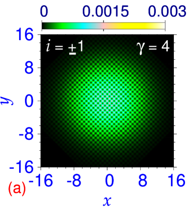
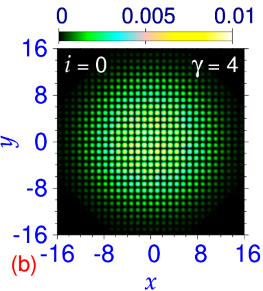
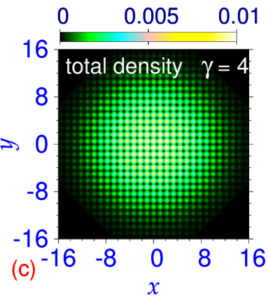
Figure 1: (Color online) Contour plot of density $n_{i}$ of the state (34) for $\gamma=4$ and $\eta=+1$ of components (a) $i=\pm 1$, (b) $i=0$, and (c) total density after replacing the factor $\sqrt{n}$ by an appropriate Gaussian distribution. The densities are normalized as $\int dxdy(n_{+1}+n_{0}+n_{-1})=1$. Results in all figures are plotted in dimensionless units.

The SO-coupled symbiotic solitons studied in this paper are localized states, whereas the solutions (32)-(34) of the single-particle Hamiltonian are not localized. However, if we multiply these by an appropriate localized 2D Gaussian state we can generate states quite similar to those of localized stripe and superlattice solitons. This is illustrated in Fig. 1 through a contour plot of density of the state (34) for $\gamma=4$ and $\eta=1$ of components (a) $i=\pm 1$, (b) $i=0$ and (c) total density after replacing the factor $\sqrt{n}$ by an appropriate Gaussian. The density of this state is quite similar to a superlattice soliton with square-lattice pattern in density for $\gamma=4,c_{0}=1,c_{2}=-2,$ viz. Figs. 6(a)-(c). Even the total density in Fig. 1(c) has a square-lattice pattern as in a superlattice BEC. Hence an analytic consideration of the single-particle Hamiltonian reveals that it can naturally lead to eigenstates with densities quite similar to an actual stripe and superlattice soliton of an SO-coupled spin-1 BEC. In a weakly-attractive uniform system, that we consider in this paper, the energies of these states are very close to the analytic energy $e=-\gamma^{2}/2$ of the states (32) and (34) in most cases, indicating a negligible contribution from the nonlinear terms $c_{0}$ and $c_{2}$.

III Result and Discussion

We numerically solve the coupled partial differential GP equations using the split-time-step Crank-Nicolson method Muruganandam with real- and imaginary-time propagation. For a numerical simulation there are the FORTRAN Muruganandam and C cc programs for the solution of the GP equation and their open-multiprocessing omp version appropriate for SO-coupled spin-1 spinor BEC. The real-time propagation method was used to study the dynamics with the converged solution obtained in imaginary-time propagation as the initial state. The space step employed for the solution of Eqs. (8) and (15) to obtain the quasi-1D symbiotic solitons by the imaginary- and real-time propagation is $dx=0.0125$ and that for the solution of Eqs. (27) and (30) to obtain the quasi-2D symbiotic SO-coupled spinor soliton by the imaginary- and real-time propagation is $dx=dy=0.05$. In both quasi-1D and quasi-2D cases the time step for imaginary-time propagation is $dt=0.1dx^{2}$ and for real-time propagation is $dt=0.05dx^{2}$.

Instead of presenting results only in dimensionless units, we will also relate the results with the most commonly used ferromagnetic ⁸⁷Rb atom with the scattering lengths a0a2 $a_{0}=101.8a_{B}$ and $a_{2}=100.4a_{B}$ satisfying $c_{0}>0$ and $c_{2}<0$, where $a_{B}$ is the Bohr radius. In all experiments on solitons li ; rb the actual value of scattering length was modified by the Feshbach-resonance technique Inouye so as to have a reasonable number of atoms in the soliton in the harmonic trap used in a laboratory. Similarly, we will consider a modified value of $a_{2}$ of ⁸⁷Rb atoms, obtained by the Feshbach-resonance technique in this paper: $a_{2}=-20.36a_{B}$, appropriate for both quasi-1D and quasi-2D cases, as we will see in the following.

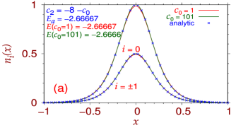
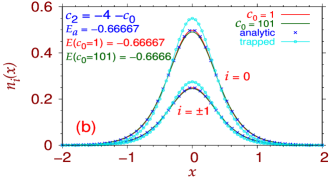
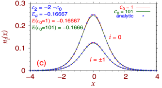
Figure 2: (Color online) Numerical (lines) and analytic (points) densities $n_{i}(x),i=0,\pm 1,$ of the three components for the lowest-energy symbiotic vector soliton with $c_{0}=1$ and 101 and (a) $c_{0}+c_{2}=-8$, (b) $c_{0}+c_{2}=-4$, and (c) $c_{0}+c_{2}=-2$. Numerical energy $E$ and analytic energy $E_{a}$ of Eq. (23) are also shown. All quantities in this and following figures are dimensionless.

III.1 Stationary soliton

III.1.1 Quasi-1D symbiotic spin-1 spinor soliton

For the formation of a quasi-1D symbiotic spin-1 spinor soliton we consider $c_{0}>0$ and $c_{2}<0,$ such that $c_{0}+c_{2}<0$. In this case, magnetization is conserved (in absence of SO coupling), hence, in the imaginary-time propagation, we consider an initial state with the property $n_{+1}(x)=n_{-1}(x)$ $(m=0)$, so that the converged final state also has the same property as required of a quasi-1D symbiotic spin-1 spinor soliton. The soliton profile is found to be reasonably insensitive to a variation of $c_{0}$ provided that $c_{0}+c_{2}$ is kept fixed, in agreement with the analytic result (22). We demonstrate this considering $c_{0}=1$ and 101 corresponding to self repulsion. In Fig. 2(a) we illustrate the component densities of the symbiotic soliton for $c_{0}+c_{2}=-8$ and $c_{0}=1$ and 101. The analytic density (point) and numerical density (line) as well as the corresponding energies are shown for both $c_{0}=1$ and 101. The analytic energy $E_{a}$ of Eq. (23) is independent of $c_{0}$, provided $|c_{0}+c_{2}|$ is unchanged, and is in good agreement with the numerical energy $E$. The numerical energies of the quasi-1D symbiotic solitons in Fig. 2 are converged results without numerical error. In Figs. 2(b) and (c) we display the densities for $c_{0}+c_{2}=-4$ and $-2$, respectively, and $c_{0}=1$ and 101. As the value of $|c_{0}+c_{2}|$ decreases from 8 to 2, the net attraction is reduced, consequently, the soliton occupies a larger extension of space as illustrated in Fig. 2. In all cases, as $c_{0}$ increases, the numerical energy increases for a fixed $|c_{0}+c_{2}|$. In all cases, as required, $n_{+1}(x)=n_{-1}(x)$.

Let us now see if the symbiotic solitons displayed in Fig. 2 are feasible in an actual experiment with ⁸⁷Rb atoms with Feshbach-modified scattering lengths $a_{0}=101.8a_{B}$ and $a_{2}=-20.36a_{B}$. Equation (9) relates the nonlinearities with the number of atoms, scattering lengths and trap parameter. If we take in Eq. (9) the parameters $l_{yz}=l_{0}=2$ $\mu$m and the number of atoms $N=3710$ then we obtain $c_{0}=4$ and $c_{2}=-8=-4-c_{0}$; these nonlinearity parameters with $101>c_{0}>1$ correspond to the scenario of Fig. 2(b). The parameter $l_{yz}\equiv\sqrt{\hbar/M\omega_{yz}}=2$ $\mu$m, with $M$ the mass of a ⁸⁷Rb atom, yields the average harmonic trap frequency in the $y-z$ plane: $\omega_{yz}\approx 2\pi\times 29$ Hz.

III.1.2 Quasi-2D symbiotic SO-coupled spin-1 soliton

Next we consider the formation of a quasi-2D symbiotic SO-coupled spin-1 spinor soliton. For a small $\gamma$, these solitons are of the $(\mp 1,0,\pm 1)$ type kita where the upper (lower) sign corresponds to Rashba (Dresselhaus) SO coupling. In quasi-2D setting, Eq. (28) relates the nonlinearities with the number of atoms, scattering lengths and trap parameter. If in Eq. (28) we take the trap parameter $l_{z}=\sqrt{2\pi}$ $\mu$m, number of atoms $N=465,$ then we obtain $c_{0}=1$ and $c_{2}=-2$; we will take these nonlinearity parameters in the study of quasi-2D symbiotic SO-coupled soliton in this paper. In case of ⁸⁷Rb atoms with Feshbach-modified scattering lengths $a_{0}=101.8a_{B}$ and $a_{2}=-20.36a_{B}$, the parameter $l_{z}\equiv\sqrt{\hbar/M\omega_{z}}=\sqrt{2\pi}$ $\mu$m leads to the following harmonic trap frequency in the $z$ direction: $\omega_{z}\approx 2\pi\times 18.5$ Hz.

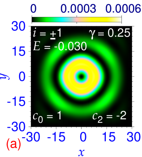
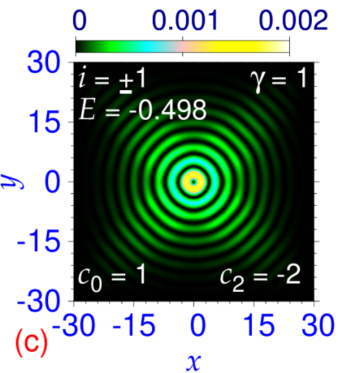
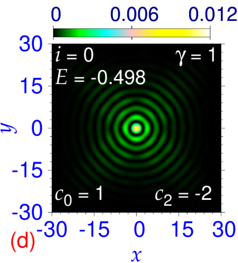
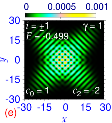
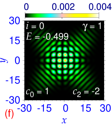
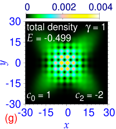
Figure 3: (Color online) Contour plot of density $n_{i}$ of a $(\mp 1,0,\pm 1)$-type quasi-2D symbiotic Rashba or Dresselhaus SO-coupled spin-1 spinor soliton of components (a) $i=\pm 1$, (b) $i=0$ with parameters $c_{0}=1,c_{2}=-2,\gamma=0.25$ and of a multi-ring soliton of components (c) $i=\pm 1$, (d) $i=0$ with parameters $c_{0}=1,c_{2}=-2,\gamma=1$. The same of a superlattice soliton with parameters $c_{0}=1,c_{2}=-2,\gamma=1$ of components (e) $i=\pm 1$, (f) $i=0$ and (g) total density.

In Fig. 3 we display the contour plot of density of components (a) $i=\pm 1$ and (b) $i=0$ of a $(\mp 1,0,\pm 1)$-type soliton for parameters $c_{0}=1,c_{2}=-2,\gamma=0.25$. There is one prominent ring in this case. The numerical energy ($E=-0.030\approx-\gamma^{2}/2=-0.03125$) and the density of the $(\mp 1,0,\pm 1)$-type soliton in Figs. 3(a)-(b) are independent of the type of SO coupling: Rashba or Dresselhaus. The estimated numerical error in energy for all quasi-2D solitons reported in this paper is small ($\sim\pm 0.001$). In the numerical calculation by imaginary-time propagation, the vortex-antivortex structure was imprinted in the respective initial wave function components.

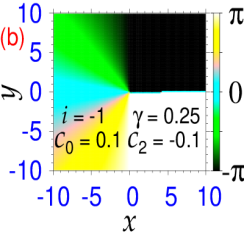
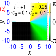
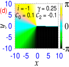
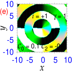
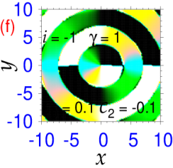
Figure 4: (Color online) Contour plot of the phase of the wave function of the symbiotic soliton shown in Figs. 3(a)-(b) for Rashba SO coupling of components (a) $i=+1$ and (b) $i=-1$. The same of the symbiotic soliton shown in Figs. 3(a)-(b) for Dresselhaus SO coupling of components (c) $i=+1$ and (d) $i=-1$. Contour plot of the phase of the wave function of the symbiotic soliton shown in Figs. 3(c)-(d) for Rashba SO coupling of components (e) $i=+1$ and (f) $i=-1$.

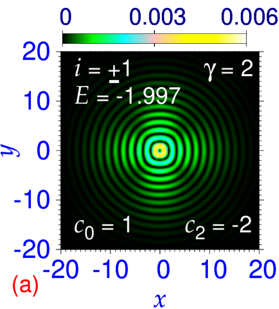
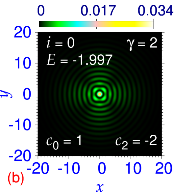
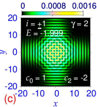
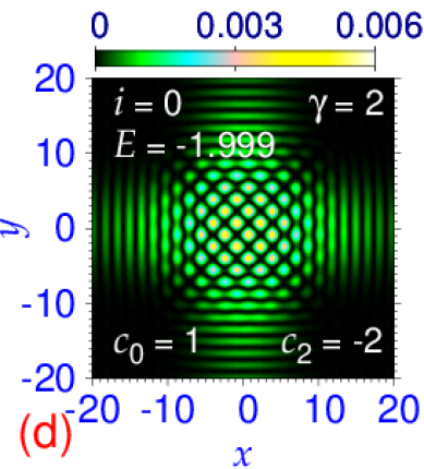
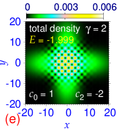
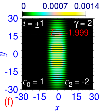
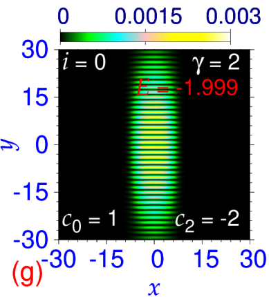
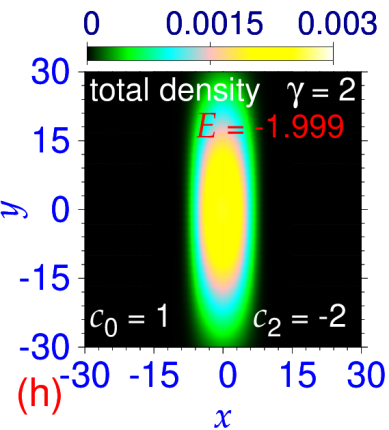
Figure 5: (Color online) Contour plot of density $n_{i}$ of a quasi-2D multi-ring spin-1 Rashba or Dresselhaus SO-coupled symbiotic BEC soliton of components (a) $i=\pm 1$ and (b) $i=0$; the same of a superlattice soliton of components (c) $i=\pm 1$, (d) $i=0,$ and (e) the total density; the same of a stripe soliton of components (f) $i=\pm 1$, (g) $i=0,$ and (h) the total density. In all cases $c_{0}=1,c_{2}=-2,\gamma=2$.

As $\gamma$ is increased, a multi-ring structure appears in the densities of a $(\mp 1,0,\pm 1)$-type quasi-2D symbiotic SO-coupled spin-1 spinor soliton as illustrated in Fig. 3 for $\gamma=1$ through a contour plot of density of components (c) $i=\pm 1$, (d) $i=0$ for parameters $c_{0}=1,c_{2}=-2$. In addition to the multi-ring symbiotic soliton, we find a new type of quasi-degenerate superlattice symbiotic soliton as shown in Fig. 3 for $\gamma=1$, where we display a contour plot of densities of components (e) $i=\pm 1$, (f) $i=0$ and (g) total density. In this superlattice symbiotic soliton, a square-lattice structure appears not only in the component densities, viz. Figs. 3(e)-(f), but also in the total density, viz. Fig. 3(g), thus illustrating the super-solid nature of this symbiotic soliton. In case of $\gamma=1$, the numerical energy of the superlattice soliton ($E=-0.499$) is approximately equal to the same of the multi-ring ($E=-0.498$) soliton and these two states are quasi degenerate. In the numerical calculation by imaginary-time propagation the square-lattice structure was imprinted in the respective initial wave-function components.

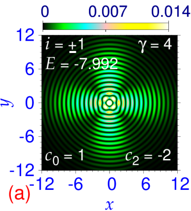
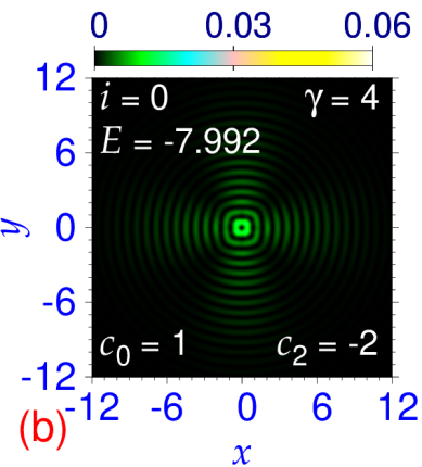
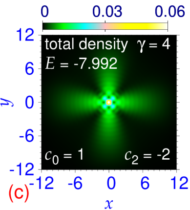
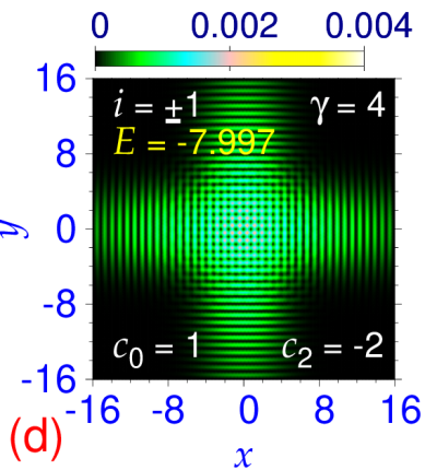
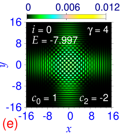
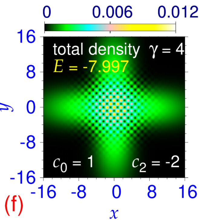
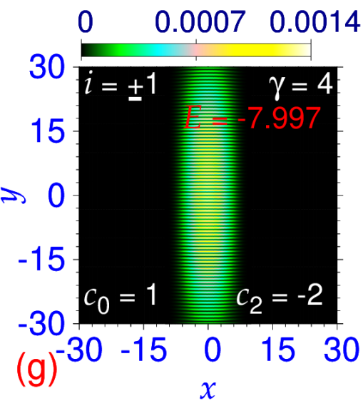
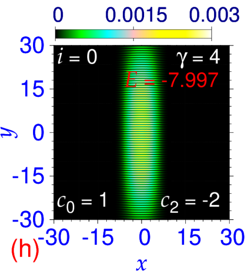
Figure 6: (Color online) Contour plot of density $n_{i}$ of a quasi-2D multi-ring spin-1 Rashba or Dresselhaus SO-coupled symbiotic BEC soliton of components (a) $i=\pm 1$, (b) $i=0$ and (c) total density; the same of a superlattice soliton of components (d) $i=\pm 1$, (e) $i=0$, and (f) the total density; the same of a stripe soliton of components (g) $i=\pm 1$ and (h) $i=0$. In all cases $c_{0}=1,c_{2}=-2,\gamma=4$.

The presence of the vortices in the component densities of Figs. 3(a)-(d) can be confirmed from a study of the phase of the respective wave functions. In Fig. 4 we show a contour plot of the phase of the wave-function components (a) $i=+1$ and (b) $i=-1$ of the soliton of Figs. 3(a)-(b) for $\gamma=0.25$ for Rashba SO coupling. The same for Dresselhaus SO coupling is shown in Figs. 4 (c) $i=+1$ and (d) $i=-1$. In Fig. 4(a) there is a phase drop of $-2\pi$ upon a complete rotation around the center corresponding to an antivortex of unit angular momentum at the center of component $i=+1$ for Rashba SO coupling. In Fig. 4(b) the phase drop is $+2\pi$ corresponding to a vortex of unit angular momentum at the center of component $i=-1$. The phase drops upon a complete rotation around the center for Dresselhaus SO coupling in Figs. 4(c)-(d) are of opposite sign compared to those in Figs. 4(a)-(b) for Rashba SO coupling, respectively, corresponding to a vortex (antivortex) of unit angular momentum in component $i=+1$ ($i=-1$). A contour plot of the phase of the wave function of components $i=+1$ and $i=-1$ of the soliton of Figs. 3(c)-(d) for Rashba SO coupling with $\gamma=1$ is displayed in Figs. 4(e)-(f). From the plots in Figs. 4(e) and (f) we confirm a phase drop of $-2\pi$ and $2\pi$, respectively, at the center corresponding to an antivortex (vortex) in component $i=+1$ ($i=-1$) for Rashba coupling. The phase drop for Dresselhaus coupling for $\gamma=1$ is of opposite sign, compared to Rashba coupling, corresponding to a vortex (antivortex) at the center of component $i=+1$ ($i=-1$) (not shown in this paper).

In Fig. 5 we display the density of components (a) $i=\pm 1,$ and (b) $i=0$ of a $(\mp 1,0,\pm 1)$-type quasi-2D symbiotic multi-ring soliton for $c_{0}=1,c_{2}=-2$ and $\gamma=2$. The circular symmetry of this multi-ring soliton is partially broken with the increase of $\gamma$. In Fig. 5 the density of components (c) $i=\pm 1,$ (d) $i=0$ and (e) total density of the superlattice soliton for the same parameters is presented. In this case we also display in Fig. 5 the contour plot of the density of the stripe soliton of components (f) $i=\pm 1$, (g) $i=0$, and (h) the total density. The total density in this case does not have any spatially-periodic modulation. The energy of the multi-ring, superlattice and stripe solitons are $E=-1.997,-1.999$ and $E=-1.999$ ($\approx-\gamma^{2}/2=-2$), respectively, so that the superlattice and the stripe solitons are quasi degenerate ground states and the multi-ring soliton is a metastable excited state.

In Fig. 6 we present the density of components (a) $i=\pm 1$, (b) $i=0$ and (c) total density of the symbiotic multi-ring soliton for $c_{0}=1,c_{2}=-2$ and $\gamma=4$. The circular symmetry of this multi-ring soliton is broken with the increase of $\gamma$. The density of the circularly symmetric $\gamma=4$ state of Figs. 6(a)-(c) has acquired a four-wing shape. In Fig. 6 the density of components (d) $i=\pm 1$, (e) $i=0$ and (f) total density of the symbiotic superlattice soliton for $c_{0}=1,c_{2}=-2$ and $\gamma=4$ is displayed. In Fig. 6 the density of components (g) $i=\pm 1,$ and (h) $i=0$ of the symbiotic stripe soliton for the same parameters is presented. The total density (not shown here) of the stripe soliton does not have any spatially-periodic modulation. The energies of the multi-ring, superlattice and stripe solitons are $E=-7.992,E=-7.997,E=-7.997$ ($\approx-\gamma^{2}/2=-8$), respectively, so that the superlattice and the stripe solitons continue as quasi-degenerate ground states for large SO coupling. The results of density and energy presented in Fig. 3, 5 and 6 remain the same for both Rashba and Dresselhaus SO couplings, although the complex wave functions for these SO couplings are different.

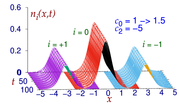
Figure 7: (Color online) Density profile of the quasi-1D symbiotic spin-1 spinor soliton $n_{i}(x,t)$ of Fig. 2(b) versus $x$ and $t$ during real-time propagation demonstrating its dynamical stability. For a better view of the individual components, the component densities are plotted after a spatial displacement among these. The initial wave function was obtained by imaginary-time simulation with parameters $c_{0}=1,c_{2}=-5,$ and the real-time propagation using that initial wave function was executed after changing $c_{0}$ from 1 to 1.5 at $t=0$.

In fact, with the increase of SO coupling, the $(\mp 1,0,\pm 1)$-type multi-ring soliton for $\gamma=4$, viz. Figs. 6(a)-(c), has turned to an excited metastable state form a stable ground state for $\gamma=0.25$, viz. Figs. 3(a)-(b). In imaginary-time propagation, after a very large number of time iterations, the multi-ring soliton becomes the ground superlattice soliton of Figs. 6(d)-(f). The total density of the metastable multi-ring soliton of Fig. 6(c), after a reasonably large number of iterations, has already acquired a square-lattice structure in the central region resembling a superlattice soliton, indicating the beginning of a spontaneous transition to a superlattice state. Hence, as the SO coupling increases, the $(\mp 1,0,\pm 1)$-type solitons spontaneously break the rotational symmetry and become superlattice solitons. It seems natural that the superlattice solitons can be generated in imaginary-time propagation from a square-lattice imprinted initial state (34). But the fact that the use of a $(\mp 1,0,\pm 1)$-type initial state for large SO coupling also leads to a superlattice soliton after a very large number of time iterations establishes the superlattice soliton as the robust ground state for large SO coupling, independent of finite system size and boundary condition, with the stripe soliton, with completely different symmetry, appearing as a quasi-degenerate state.

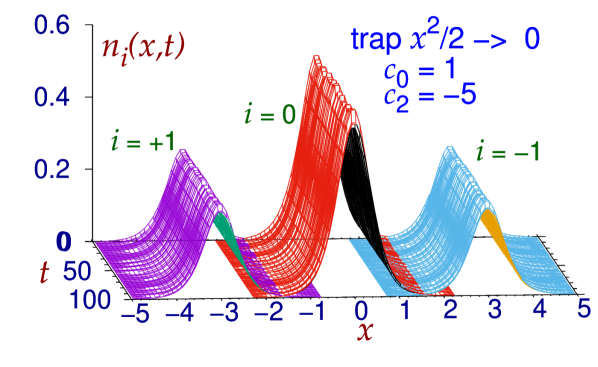
Figure 8: (Color online) Density profile of a quasi-1D trapped symbiotic BEC $n_{i}(x,t)$ with $c_{0}=1,c_{2}=-5$, viz. Fig. 2(b), versus $x$ and $t$ during real-time propagation after suddenly removing the trap $V(x)=x^{2}/2$ at $t=0$. The initial wave function in real-time propagation is the converged imaginary-time wave function. For a better view of the individual components, the component densities are plotted after a spatial displacement among these.

III.2 Dynamical stability

III.2.1 Quasi-1D symbiotic spin-1 soliton

To demonstrate that the symbiotic vector soliton is dynamically stable we subject the ground-state vector soliton profile, obtained by imaginary-time simulation, to real-time propagation for a long time after giving a perturbation by changing the interaction strength $c_{0}$ slightly at time $t=0$. The profile of the vector soliton is sensitive to $c_{0}$. For this purpose, we consider the quasi-1D symbiotic vector soliton displayed in Fig. 2(b) obtained with parameters $c_{0}=1,c_{2}=-5$. The real-time propagation during 100 time units for this soliton was executed upon changing the interaction strength $c_{0}$ from 1 to 1.5 at time $t=0$. In Fig. 7 we exhibit the density profile of the three components of the vector soliton during real-time propagation. For a better view, we have displaced the density profile of components $i=+1$ and $i=-1$ to $x=-3$ and $x=+3$, respectively, leaving the $i=0$ component at $x=0$. The long-time stable propagation of the components of the vector soliton establishes its dynamical stability.

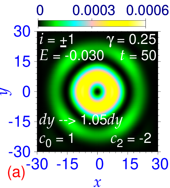
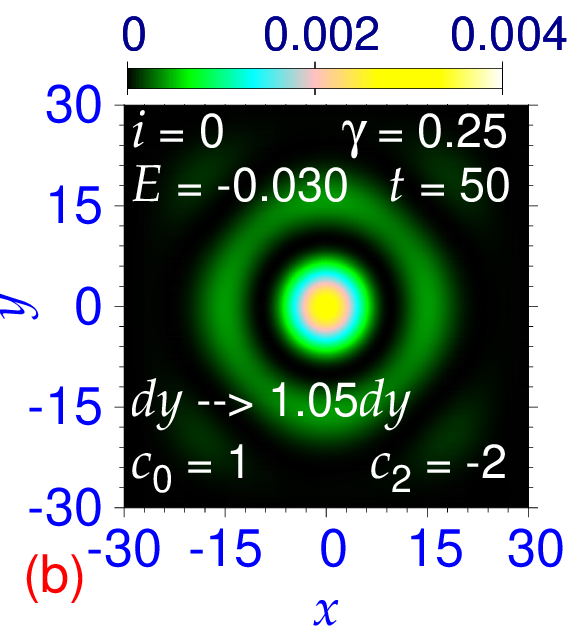
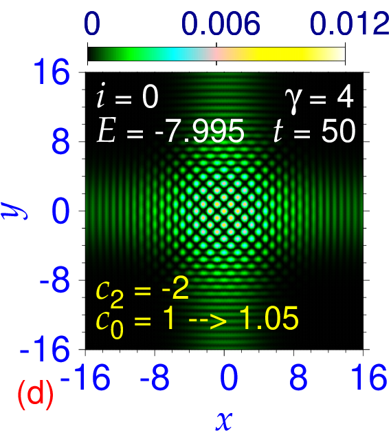
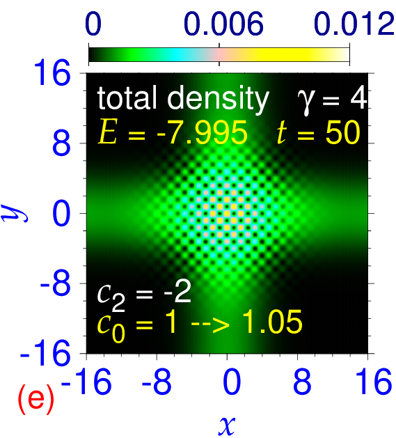
Figure 9: (Color online) Contour plot of density of the quasi-2D symbiotic SO-coupled $(-1,0,+1)$-type soliton with Rashba coupling, displayed in Figs. 3(a)-(b), of components (a) $i=\pm 1$ and (b) $i=0$ after real-time propagation at time $t=50$ with a deformed wave function (see text for details); the same of the superlattice symbiotic BEC soliton, of Figs. 6(d)-(f), of components (c) $i=\pm 1$, (d) $i=0$ and (e) the total density, after real-time propagation at time $t=50$ upon a change of the nonlinearity coefficient $c_{0}$ from 1 to 1.05 at $t=0$.

Now we demonstrate the possibility of the creation of the quasi-1D symbiotic soliton of Fig. 2(b) in a laboratory. For this purpose we consider a quasi-1D symbiotic spin-1 BEC in a trap $V(x)=x^{2}/2$. First we consider the formation of this trapped BEC with $c_{0}=1$ and $c_{2}=-5$ by imaginary-time propagation. The density of this trapped BEC is plotted in Fig. 2(b). The resultant density is quite close to that of the untrapped soliton shown in this plot. After creation, this trapped BEC is subjected to real-time propagation upon suddenly removing the confining trap at time $t=0$. The steady real-time propagation of the resultant system for 100 units of time shown in Fig. 8 demonstrates both the dynamical stability of the symbiotic spin-1 soliton and the plausibility of the creation of the same in a laboratory.

III.2.2 Quasi-2D symbiotic SO-coupled spin-1 soliton

To demonstrate the dynamical stability of a quasi-2D symbiotic SO-coupled spin-1 spinor soliton, we consider the $(-1,0,+1)$-type soliton of Figs. 3(a)-(b) and the superlattice soliton of Figs. 6(d)-(f), using Rashba coupling. Of these, the $(-1,0,+1)$-type soliton of Figs. 3(a)-(b) hosting vortices is of special concern as vortices may exhibit transverse instability arising from a deformation of the wave function. To check the stability of this $(-1,0,+1)$-type soliton, we deform the soliton wave function slightly, so that the isodensity lines of Figs. 3(a)-(b) are distorted to have an approximate elliptic shape, by increasing the space discretization step in the $y$ direction $dy$ by a factor of 1.05. Then we subject the imaginary-time wave function in this deformed space to real-time propagation during 50 units of time. The resultant density of the $(-1,0,+1)$-type SO-coupled quasi-2D soliton at $t=50$, displayed in Fig. 9 for components (a) $i=\pm 1$ and (b) $i=0$, does not exhibit any transverse instability. Starting from a radially-deformed shape the $(-1,0,+1)$-type soliton has settled to its original circular-symmetric shape.

To check the stability of the superlattice soliton of Figs. 6(d)-(f), we subject the imaginary-time wave function to real-time propagation during 50 units of time after changing the intraspecies nonlinearity coefficient $c_{0}$ from 1 to 1.05 at time $t=0$. The resultant density of the superlattice soliton is displayed in Fig. 9 for components (c) $i=\pm 1$, (d) $i=0$, and (e) total density. In both cases, although the root-mean-square sizes and energy were oscillating a little during real-time propagation, the prominent pattern in density survived at $t=50$ as can be seen in Fig. 9. If the solitons were not dynamically stable, the vortex and superlattice structure of the wave functions would have been destroyed after real-time propagation.

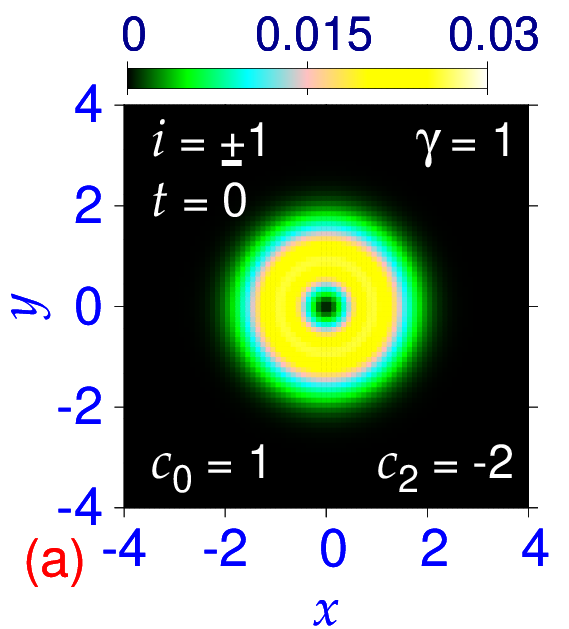
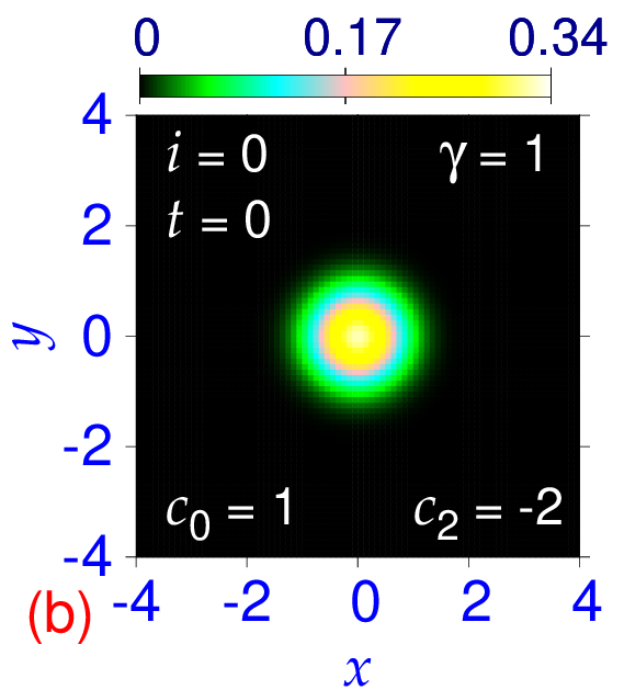
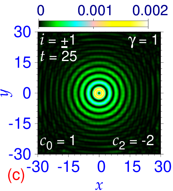
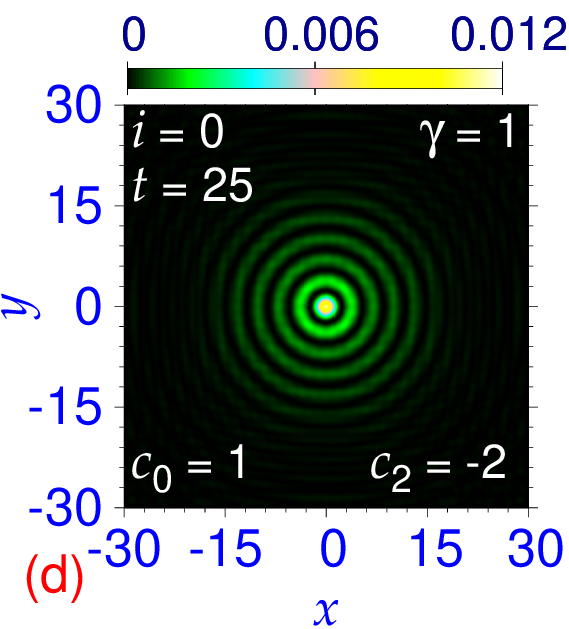
Figure 10: (Color online) Contour plot of density of a quasi-2D symbiotic SO-coupled $(-1,0,+1)$-type trapped BEC with Rashba coupling, of components (a) $i=\pm 1$ and (b) $i=0$ at $t=0$; the same of the generated $(-1,0,+1)$-type multi-ring soliton after real-time propagation at time $t=25$ of components (c) $i=\pm 1$ and (d) $i=0$, upon a sudden removal of the trap at $t=0$. The parameters of simulation: $c_{0}=1,c_{2}=-2,\gamma=1$

Finally, we consider the possibility of the creation of a quasi-2D $(\mp 1,0,\pm 1)$-type multi-ring symbiotic soliton of Figs. 3(c)-(d) in a laboratory. For this purpose we prepare a quasi-2D symbiotic spin-1 BEC, in a trap $V({\bf r})=r^{2}/2$, with parameters $c_{0}=1$ and $c_{2}=-2$ and Rashba SO-coupling strength $\gamma=1$, by imaginary-time propagation. The contour plot of density of this trapped BEC is plotted, in Fig. 10, of components (a) $i=\pm 1$ and (b) $i=0$. After creation, this trapped BEC is subjected to real-time propagation upon a sudden removal of the confining trap at time $t=0$. A snapshot of the contour density of the generated soliton at time $t=25$ is displayed, in Fig. 10, of components (c) $i=\pm 1$ and (d) $i=0$. During real-time propagation the size of the BEC has increased by a factor of 10, while the rings were generated and the BEC was being transformed to a multi-ring soliton. The generated soliton is quite similar to the same of Figs. 3(c)-(d), which demonstrates the robustness and stability of this soliton.

IV Summary

We studied the formation of quasi-1D and quasi-2D symbiotic spin-1 spinor solitons in a self-repulsive spin-1 BEC using a numerical solution and an analytic approximation of the underlying mean-field GP equation with two nonlinear parameters $c_{0}$ and $c_{2}$. A symbiotic soliton with intraspecies repulsion and interspecies attraction should necessarily require $c_{0}>0$ and $c_{2}<0$. Even then there is a self-attractive term proportional to $c_{2}n_{\pm}\psi_{\pm}$ in components $i=\pm 1$, viz. Eqs. 7 and 26. This inappropriate self-attractive term can be avoided if we further impose the condition $n_{+1}=n_{-1}$, so that Eqs. 7 and 26 reduce to Eqs. 15 and 30, respectively. Consequently, solutions of Eqs. 15 and 8, and Eqs. 30 and 27, in quasi-1D and quasi-2D configurations, respectively, are appropriate for the study of symbiotic quasi-1D and quasi-2D spin-1 solitons with the property $n_{+1}=n_{-1}$. In the quasi-1D case the numerical result for density and energy of the symbiotic spin-1 spinor soliton are in good agreement with an analytic approximation.

In the quasi-2D case, in addition, a non-zero SO coupling is necessary for the formation of a symbiotic spin-1 BEC soliton. For a small strength $\gamma$ of SO coupling, the quasi-2D symbiotic SO-coupled spin-1 spinor soliton is of the $(\mp 1,0,\pm 1)$ type with multi-ring structure hosting vortices of vorticity $\mp 1$ and $\pm 1$ in components $i=+1$ and $-1$, respectively, where the upper (lower) sign refer to Rashba (Dresselhaus) SO coupling. For large strength of SO coupling, in addition to the above multi-ring symbiotic solitons there appear quasi-degenerate stripe solitons and superlattice solitons. The superlattice solitons have square-lattice structure in component and total densities, thus sharing properties of a supersolid. For larger SO coupling, the $(\mp 1,0,\pm 1)$-type multi-ring soliton becomes an excited metastable state and spontaneously breaks the rotational symmetry to become a stable superlattice soliton. The superlattice and the stripe solitons continue as quasi-degenerate ground states. An SO-coupled quasi-1D spin-1 BEC naturally leads to an 1D periodic pattern in density 29 ; hence an SO-coupled quasi-2D BEC involving two perpendicular SO-coupling directions, as considered in this paper, should naturally lead to a square-lattice structure in density in addition to the stripe pattern. We could not rule out the possibility of the appearance of a triangular-lattice or other structure, although we could not find out any other stable periodic structure in this study. In all cases, the energy and density of the quasi-2D symbiotic soliton are the same for both Rashba and Dresselhaus SO couplings although the two complex wave functions are different. The dynamical stability of the quasi-1D and quasi-2D symbiotic spin-1 spinor solitons is demonstrated numerically by real-time propagation over a long period of time. The plausibility of the formation of a symbiotic spin-1 BEC soliton in a laboratory by removing the trap of a spin-1 trapped BEC is also demonstrated.

- (1) Y. S. Kivshar and B. A. Malomed, Rev. Mod. Phys. 61, 763 (1989); F. K. Abdullaev, A. Gammal, A. M. Kamchatnov, and L. Tomio, Int. J. Mod. Phys. B 19, 3415 (2005).
- (2) K. E. Strecker, G. B. Partridge, A. G. Truscott, and R. G. Hulet, Nature (London) 417, 150 (2002); L. Khaykovich, F. Schreck, G. Ferrari, T. Bourdel, J. Cubizolles, L. D. Carr, Y. Castin, and C. Salomon, Science 256, 1290 (2002).
- (3) S. L. Cornish, S. T. Thompson, and C. E. Wieman, Phys. Rev. Lett. 96, 170401 (2006).
- (4) S. Inouye, M. R. Andrews, J. Stenger, H.-J. Miesner, D. M. Stamper-Kurn, and W. Ketterle, Nature (London) 392, 151 (1998).
- (5) V. M. Pérez-García and J. B. Beitia, Phys. Rev. A 72, 033620 (2005); S. K. Adhikari, Phys. Lett. A 346, 179 (2005).
- (6) D. M. Stamper-Kurn, M. R. Andrews, A. P. Chikkatur, S. Inouye, H.-J. Miesner, J. Stenger, and W. Ketterle, Phys. Rev. Lett. 80, 2027 (1998).
- (7) J. Ieda, T. Miyakawa, and M. Wadati, Laser Phys. 16, 678 (2006); J. Ieda, T. Miyakawa, and M. Wadati, Phys. Rev. Lett. 93, 194102 (2004); L. Li, Z. Li, B. A. Malomed, D. Mihalache, and W. M. Liu, Phys. Rev. A 72, 033611 (2005); W. Zhang, Ö. E. Müstecaplioǧlu, and L. You, Phys. Rev. A 75, 043601 (2007); B. J. Dąbrowska-Wüster, E. A. Ostrovskaya, T. J. Alexander, and Y. S. Kivshar, Phys. Rev. A 75, 023617 (2007); E. V. Doktorov, J. Wang, and J. Yang, Phys. Rev. A 77, 043617 (2008); B. Xiong and J. Gong; Phys. Rev. A 81, 033618 (2010); P. Szankowski, M. Trippenbach, E. Infeld, and G. Rowlands, Phys. Rev. Lett. 105, 125302 (2010); M. Mobarak and A. Pelster, Laser Phys. Lett. 10, 115501 (2013); O. Topic, M. Scherer, G. Gebreyesus, et al., Laser Phys. 20, 1156 (2010); M. Guilleumas, B. Julia-Diaz, M. Mele-Messeguer, and A. Polls, Laser Phys. 20, 1163 (2010).
- (8) L. Bergé, Phys. Rep. 303, 259 (1998); R. Y. Chiao, E. Garmire, and C. H. Townes, Phys. Rev. Lett. 13, 479 (1964); S. K. Adhikari, Phys. Rev. A69, 063613 (2004); C.-A. Chen and C.-L. Hung, Phys. Rev. Lett. 125, 250401 (2020).
- (9) H. Sakaguchi, B. Li, B. A. Malomed, Phys. Rev. E 89, 032920 (2014); H. Sakaguchi and B. A. Malomed, Phys. Rev. E 90, 062922 (2014).
- (10) Y. Xu, Y. Zhang, and B. Wu, Phys. Rev. A 87, 013614 (2013); S. Cao, C.-J. Shan, D.-W. Zhang, X. Qin, and J. Xu, J. Opt. Soc. Am. B 32, 201 (2015); Lin Wen, Q. Sun, Yu Chen, Deng-Shan Wang, J. Hu, H. Chen, W.-M. Liu, G. Juzeliūnas, Boris A. Malomed, and An-Chun Ji, Phys. Rev. A 94, 061602(R) (2016); V. Achilleos, D. J. Frantzeskakis, P. G. Kevrekidis, and D. E. Pelinovsky, Phys. Rev. Lett. 110, 264101 (2013).
- (11) S. Gautam and S. K. Adhikari, Laser Phys. Lett. 12, 045501 (2015); G C Katsimiga, S I Mistakidis, P Schmelcher, and P G Kevrekidis, New J. Phys. 23, 013015 (2021).
- (12) S. Gautam and S. K. Adhikari, Phys. Rev. A95, 013608 (2017); S. Gautam and S. K. Adhikari, Phys. Rev. A97, 013629 (2018).
- (13) V. Galitski and I. B. Spielman, Nature (London) 494, 49 (2013); J. Dalibard, F. Gerbier, G. Juzeliūnas, and P. Öhberg, Rev. Mod. Phys. 83, 1523 (2011); Y. Li, Giovanni I. Martone, and S. Stringari, Ann. Rev. Cold At. Mol. 3, Ch 5, 201 (2015) (World Scientific, 2015).
- (14) K. Osterloh, M. Baig, L. Santos, P. Zoller, and M. Lewenstein, Phys. Rev. Lett. 95, 010403 (2005); J. Ruseckas, G. Juzeliūnas, P. Öhberg, and M. Fleischhauer, Phys. Rev. Lett. 95, 010404 (2005); G. Juzeliūnas, J. Ruseckas, and J. Dalibard, Phys. Rev. A 81, 053403 (2010).
- (15) E. I. Rashba, Fiz. Tverd. Tela 2, 1224 (1960) [English Transla.: Sov. Phys. Solid State 2, 1109 (1960).]
- (16) G. Dresselhaus, Phys. Rev. 100, 580 (1955).
- (17) Y.-J. Lin, K. Jiménez-García, I. B. Spielman, Nature (London) 471, 83 (2011).
- (18) J. Li, W. Huang, B. Shteynas, S. Burchesky, F. Ç. Top, E. Su, J. Lee, A. O. Jamison, and W. Ketterle, Phys. Rev. Lett. 117, 185301 (2016).
- (19) D. Campbell, R. Price, A. Putra, A. Valdés-Curiel, D. Trypogeorgos, and I. B. Spielman, Nat. Commun. 7, 10897 (2016).
- (20) Z. Lan and P. Öhberg, Phys. Rev. A 89, 023630 (2014); C. Wang, C. Gao, C.-M. Jian, and H. Zhai, Phys. Rev. Lett. 105, 160403 (2010)
- (21) T. Mizushima, K. Machida, T. Kita, Phys. Rev. Lett. 89, 030401 (2002); T. Mizushima, K. Machida, T. Kita, Phys. Rev. A 66, 053610 (2002).
- (22) E.P. Gross, Phys. Rev. 106, 161 (1957); A. F. Andreev and I. M. Lifshitz, Zurn. Eksp. Teor. Fiz. 56, 2057 (1969) [English Transla.: Sov. Phys. JETP 29, 1107 (1969)]; A. J. Leggett, Phys. Rev. Lett. 25, 1543 (1970); G. V. Chester, Phys. Rev. A 2, 256 (1970); M. Boninsegni and N. V. Prokof’ev, Rev. Mod. Phys. 84, 759 (2012); V. I. Yukalov, Physics 2, 49 (2020).
- (23) Zhen-Kai Lu, Yun Li, D. S. Petrov, and G. V. Shlyapnikov, Phys. Rev. Lett. 115, 075303 (2015); N. Y. Yao, C. R. Laumann, A. V. Gorshkov, S. D. Bennett, E. Demler, P. Zoller, and M. D. Lukin Phys. Rev. Lett. 109, 266804 (2012).
- (24) F. Böttcher, J.-N. Schmidt, M. Wenzel, J. Hertkorn, M. Guo, T. Langen, and T. Pfau, Phys. Rev. X 9, 011051 (2019); J. Hertkorn, F. Böttcher, M. Guo, J. N. Schmidt, T. Langen, H. P. Büchler, and T. Pfau, Phys. Rev. Lett. 123, 193002 (2019); L. Tanzi, E. Lucioni, F. Famà, J. Catani, A. Fioretti, C. Gabbanini, R. N. Bisset, L. Santos, and G. Modugno, Phys. Rev. Lett. 122, 130405 (2019); L. Chomaz, D. Petter, P. Ilzhöfer, G. Natale, A. Trautmann, C. Politi, G. Durastante, R. M. W. van Bijnen, A. Patscheider, M. Sohmen, M. J. Mark, and F. Ferlaino, Phys. Rev. X 9, 021012 (2019); G. Natale, R. M. W. van Bijnen, A. Patscheider, D. Petter, M. J. Mark, L. Chomaz, and F. Ferlaino, Phys. Rev. Lett. 123, 050402 (2019).
- (25) J.-R. Li, J. Lee, W. Huang, S. Burchesky, B. Shteynas, F. Ç. Top, A. O. Jamison, and W. Ketterle, Nature (London) 543, 91 (2017).
- (26) Y. Li, G. I. Martone, L. P. Pitaevskii, and S. Stringari, Phys. Rev. Lett. 110, 235302 (2013); A. Putra, F. Salces-Carcoba, Y. Yue, S. Sugawa, and I. B. Spielman, Phys. Rev. Lett. 124, 053605 (2020).
- (27) S. K. Adhikari, Phys. Rev. A 103, L011301 (2021); Phys. Lett. A 388, 127042 (2021); J. Phys.: Consens. Matter 33, 265402 (2021).
- (28) Y. Kawaguchi and M. Ueda, Phys. Rep. 520, 253 (2012).
- (29) E. P. Gross, Nuovo Cimento 20, 454 (1961); L. P. Pitaevskii, Zurn. Eksp. Teor. Fiz. 40, 646 (1961) [English Transla.: Sov. Phys. JETP 13, 451 (1961).]
- (30) B. A. Malomed, Prog. Opt. 43, 71 (2002).
- (31) L. Salasnich, A. Parola, and L. Reatto, Phys. Rev. A 65, 043614 (2002).
- (32) S. Gautam and S. K. Adhikari, Phys. Rev. A 92, 023616 (2015).
- (33) P. Muruganandam and S. K. Adhikari, Comput. Phys. Commun. 180, 1888 (2009).
- (34) D. Vudragović, I. Vidanović, A. Balaž, P. Muruganandam, and S. K. Adhikari, Comput. Phys. Commun. 183, 2021 (2012).
- (35) R. Ravisankar, D. Vudragović, P. Muruganandam, A. Balaž, and S. K. Adhikari, Comput. Phys. Commun. 259, 107657 (2021); P. Kaur, A. Roy, and S. Gautam, Comput. Phys. Commun. 259, 107671 (2021).
- (36) E. G. M. van Kempen, S. J. J. M. F. Kokkelmans, D. J. Heinzen, and B. J. Verhaar, Phys. Rev. Lett. 88, 093201 (2002)